Bonferroni - based gatekeeping procedure with retesting option

Abstract

In complex clinical trials, multiple research objectives are often grouped into sets of objectives based on their inherent hierarchical relationships. Consequently, the hypotheses formulated to address these objectives are grouped into ordered families of hypotheses and thus to be tested in a pre-defined sequence. In this paper, we introduce a novel Bonferroni based multiple testing procedure for testing hierarchically ordered families of hypotheses. The proposed procedure allows the families to be sequentially tested more than once with updated local critical values. It is proved to control the global familywise error rate strongly under arbitrary dependence. Implementation of the procedure is illustrated using two examples. Finally, the procedure is extended to testing multiple families of hypotheses with a complex two-layer hierarchical structure.

1 Introduction

Complex clinical trials always involve multiple research objectives that are related in a hierarchically logical fashion based on importance, clinical relevance, and so on. Consequently, the statistical hypotheses formulated to address such objectives are grouped into hierarchically ordered families of hypotheses requiring them to be tested in a predefined sequence. Testing multiple families of hypotheses has received much attention in the last decade, and several methods have been introduced in the literature, including gatekeeping strategy (Westfall and Krishen, 2001; Dmitrienko, Offen and Westfall, 2003; Dmitrienko, Wiens and Tamhane, 2007), union closure procedures (Kim, Entsuah and Shults, 2011) and superchain procedures (Kordzakhia and Dmitrienko, 2013).

The gatekeeping strategy is a general approach developed specifically to test pre-ordered families of hypotheses in a sequential manner with each family working as a gatekeeper for the ones following it. There are several types of gatekeeping strategies available in the literature, such as serial gatekeeping strategy (Maurer, Hothorn and Lehmacher, 1995; Bauer et al. 1998; Westfall and Krishen, 2001), parallel gatekeeping strategy (Dmitrienko, Offen and Westfall, 2003), and tree gatekeeping strategy (Dmitrienko, Wiens and Tamhane, 2007; Dmitrienko et al., 2008). Based on these gatekeeping strategies, some other more powerful and flexible multiple testing methods have been developed (Chen, Luo and Capizzi, 2005; Liu and Hsu, 2009; Dmitrienko et al., 2006; Dmitrienko, Tamhane and Wiens, 2008; Dmitrienko and Tamhane, 2011; Guibaud, 2007; Bretz et al., 2009; and Burman, Sonesson and Guilbaud, 2009). For reviews on recent developments, see Dmitrienko, Tamhane and Bretz (2009), Dmitrienko, D’Agostino and Huque (2013), and Alosh, Bretz and Huque (2014).

The aforementioned gatekeeping procedures allow each family to be tested only once, which some researchers have attempted to improve. More specifically, they have added retesting options to enhance their testing powers (Guibaud, 2007; Dmitrienko, Kordzakhia and Tamhane, 2011; Dmitrienko et al., 2011; and Kordzakhia and Dmitrienko, 2013). Guilbaud (2007) incorporated the retesting option into Bonferroni based gatekeeping procedures by allowing the families to be retested in a reverse order by using procedures more powerful than the original Bonferroni procedures when all hypotheses in the last family are rejected. Dmitrienko, Kordzakhia and Tamhane (2011) improved Guilbaud’s procedure by applying some mixture procedure to each family instead of the Bonferroni procedure. In the case of testing two families, Dmitrienko et al. (2011) further improved the aforementioned procedures with retesting option by using the second family as a parallel gatekeeper instead of a serial gatekeeper for the first family; that is, as long as one hypothesis is rejected in the second family, the first family can be retested by using a more powerful procedure than the one used in the previous step. However, this procedure not only restricts to two-family case, it also requires to specify the logical relationship between each specific hypothesis in first family with each specific hypothesis in second family.

In contrast with the aforementioned sequential retesting procedures, Kordzakhia and Dmitrienko (2013) introduced a class of multiple testing procedures with retesting option on the basis of the simultaneous testing strategy, termed as superchain procedures. Unlike those sequential retesting procedures, superchain procedures test all families simultaneously at each step. Each family serves as a parallel gatekeeper for the other families. If at least one new rejection occurs in either family, the rest of the families are retested using procedures with updated critical values at the next step. Compared to the superchain procedures, the sequential retesting procedures are, however, simpler, easier to implement, and more intuitive in a clinical sense, although they have certain limitations and are restricted to some specific scenarios. In this paper, we consider overcoming such limitations and restrictions by developing newer sequential retesting procedures.

Our procedure proposed in this paper is Bonferroni based gatekeeping procedure with retesting option. However, the families are now being allowed to be retested repeatedly using Bonferroni procedures in a sequential manner with different critical value at each repetition for a family. To begin with, each family is assigned a pre-determined fraction of the overall level $\alpha$ for its initial critical value. The critical value used to test one particular family is defined as its local critical value. The level for the local critical value (referred to as local level) for a family at each test depends on certain amount of the levels associated with the local critical values passed down from higher ranked families and the initial levels assigned to lower ranked families. Each family is iteratively retested with increasingly updated local critical values.

The proposed procedure exhibits several desirable features. First, as we prove, it strongly controls the global familywise error rate (FWER), i.e., the probability of falsely rejecting at least one true null hypothesis across all families of hypotheses at a pre-specified level $\alpha$ under arbitrary dependence. Second, it is more general than the existing sequential retesting procedures since it can be constructed under almost any scenarios. And it strictly follows the hierarchical sequential scheme in the sense that higher rank families have more chances to be retested than lower rank families. Third, it is easier to implement than superchain procedure since it sticks to the simple Bonferroni method for testing each family throughout the whole procedure and proceeds in a sequential manner. Finally and interestingly, it can be described via a directed graph similar to the graphical approach (see Bretz et al., 2009), except that the nodes of the graph here represent families instead of hypotheses, and it is easy to explain the underlying testing strategy to non-statisticians.

The rest of the paper is organized as follows. In Section 2, we present some notations and definitions which are used throughout the whole paper. The main theoretical results are introduced in Section 3 including the algorithms of the proposed procedures and discussions of their global FWER control. Several special cases are discussed in Section 4 to demonstrate the relationships among the proposed procedures and some existing ones. Section 5 includes two clinical trial examples to illustrate the implementation of the proposed procedures. Section 6 extends the proposed procedures to a two-layer structure with multiple families within each layer while maintaining the control of the global FWER. Some concluding remarks are discussed in Section 7 and the Appendix gives proofs of the theoretical results.

2 Preliminary

In this section, we present some basic notations and definitions. Suppose that there are $n\geq 2$ hypotheses grouped into $m\geq 2$ ordered families, with $F_{i}=\{H_{i1},\ldots,H_{in_{i}}\}$ being the $i^{th}$ ordered family consisting of $n_{i}$ hypotheses, $i=1,\ldots,m$, $\sum_{i=1}^{m}n_{i}=n$. These hypotheses are to be tested based on their respective $p$-values $p_{ij},i=1,\ldots,m,j=1,\ldots,n_{i}$ subject to controlling an overall measure of type I error at a pre-specified level $\alpha$. Each of the true null $p$-values is assumed to be stochastically greater than or equal to the uniform distribution on $[0,1]$; that is, if $T_{i}$ is the set of true null hypotheses in $F_{i}$, then

$$\text{Pr}\left\{p_{ij}\leq u|H_{ij}\in T_{i}\right\}\leq u,i=1,\ldots,m,j=1,\ldots,n_{i},\;\mbox{for any fixed}\;u\in[0,1].$$ (1)

The familywise error rate (FWER), which is the probability of incorrectly rejecting at least one true null hypothesis, is a commonly used notion of an overall measure of type I error when testing a single family of hypotheses. Since we have multiple families, we consider this measure not locally for each family but globally. In other words, we define the global FWER as the probability of incorrectly rejecting at least one true null hypothesis across all families of hypotheses. If it is bounded above by $\alpha$ regardless of which and how many null hypotheses within each family are true, then this global FWER is said to be strongly controlled at $\alpha$.

In this paper, we propose a procedure, called Bonferroni based gatekeeping procedure with retesting option, strongly controlling the global FWER at $\alpha$. With an initial assignment of a pre-specified portion of $\alpha$, say $\alpha_{i}$, to $F_{i}$, where $\sum_{i=1}^{m}\alpha_{i}=\alpha$, the procedure starts with testing $F_{1}$ to $F_{m}$ sequentially using the Bonferroni procedure based on their own (local) critical values. The level used to locally test each family is updated from its initially assigned value to one which incorporates certain portions of the levels used in testing the previous families. After finishing a round of tests of all $m$ families, the procedure starts over for another round of tests from $F_{1}$ to $F_{m}$ again using the Bonferroni procedure based on their updated local critical values. The whole procedure stops only if there is no new rejection occurs in all $m$ families. The specific updating rule for local critical values is described in Section 3. The distribution of the amount of critical value transfered among families can be pre-fixed by an $m\times m$ transition matrix which is defined as follows.

Denote $\mathbf{G}$ = {$g_{ij}$}, $i,j=1,\ldots,m$ as a transition matrix which satisfies the following conditions:

$$0\leq g_{ij}\leq 1;\>\>g_{ij}=0,\text{ if }i=j;\>\>\sum_{j=1}^{m}g_{ij}=1,\text{ for any }i=1,\ldots,m.$$

Note that $g_{ij}$ is defined as the proportion of the critical value that can be transferred from $F_{i}$ to $F_{j}$. Figure 1 shows the graphical representation of a special case with $m=3$.

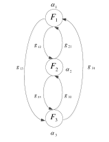
Figure 1: Three-family Bonferroni-based gatekeeping procedure with retesting option.

Remark 1

Dmitrienko, Tamhane and Wiens (2008) quantified the amount of significance level of a tested family that can be transferred to test subsequent families of hypotheses. For instance, consider testing a single family of hypotheses $F_{i}=\{H_{i1},\ldots,H_{in_{i}}\}$. Suppose it is tested using the Bonferroni procedure at level $\alpha$. Let $A_{i}$ and $R_{i}$ be the set of acceptances and rejections, respectively, with the corresponding cardinalities $|A_{i}|$ and $|R_{i}|$. Then, $\frac{|A_{i}|}{n_{i}}\alpha$ can be considered as a conservative estimate of the FWER of the Bonferroni procedure. Thus, the used and unused parts of level $\alpha$ are $\frac{|A_{i}|}{n_{i}}\alpha$ and $\frac{|R_{i}|}{n_{i}}\alpha$, respectively. The unused part, $\frac{|R_{i}|}{n_{i}}\alpha$, can be recycled to test the subsequent families of hypotheses.

3 Main results

This section presents our proposed Bonferroni-based gatekeeping procedure with retesting option. We will begin with a simple case of two families of null hypotheses in Section 3.1. The general case of an arbitrary number of families will be introduced in Section 3.2. Section 3.3 discusses the main property of the proposed procedure, which is the global FWER control.

3.1 Two - family problem

Consider multiple testing of two families of null hypotheses, $F_{i},i=1,2$, which are pre-ordered based on their hierarchical relationship. Initially, we assign $\alpha_{1}$ and $\alpha_{2}$ to $F_{1}$ and $F_{2}$, respectively, where $\alpha_{1}+\alpha_{2}=\alpha$. We let $\alpha_{1(j)}$ and $\alpha_{2(j)}$, $j\geq 1$ be the levels for the updated local critical values used for testing $F_{1}$ and $F_{2}$ at the $j^{th}$ time. The transition matrix is given by

$$\mathbf{G}=\left(\begin{array}[]{cc}0&1\\ 1&0\end{array}\right),$$

i.e., $g_{12}=g_{21}=1$, which implies the whole amount of local critical value of one family that can be recycled is transferred to test the other family. The graphical representation of this case is shown in Figure 2.

Figure 2: Two - family Bonferroni - based gatekeeping procedure with retesting option.

Denote $R_{1(j)}$ and $R_{2(j)}$, respectively, the sets of rejected nulls when $F_{1}$ and $F_{2}$ are tested at the $j^{th}$ time, while $|R_{1(j)}|$ and $|R_{2(j)}|$ are their corresponding cardinalities. The proposed Bonferroni-based gatekeeping procedure with retesting option in the case of $m=2$ is defined in the following.

Algorithm 1

Stage 1. Test $F_{1}$ at its local critical value based on the level $\alpha_{1(1)}=\alpha_{1}$ using the Bonferroni procedure, and then do the same for $F_{2}$ at the level

$$\alpha_{2(1)}=\alpha_{2}+\frac{|R_{1(1)}|}{n_{1}}\alpha_{1}.$$

If no null hypotheses are rejected in both families, the algorithm stops. Otherwise, it proceeds to the next stage.

Stage $\bm{k(k\geq 2)}$. Retest $F_{1}$ at its local critical value based on

$$\alpha_{1(k)}=\alpha_{1}+\frac{|R_{2(k-1)}|}{n_{2}}\alpha_{2},$$ (2)

using the Bonferroni procedure, and then do the same for $F_{2}$ at the level

$$\alpha_{2(k)}=\alpha_{2}+\frac{|R_{1(k)}|}{n_{1}}\alpha_{1(k)}.$$ (3)

If no new null hypotheses are rejected in both families, the algorithm stops. Otherwise, it proceeds to the next stage.

Remark 2

Algorithm 1 allows iteratively retesting $F_{1}$ and $F_{2}$ using the Bonferroni procedure at increasingly updated local levels. The amount of increased local level of $F_{1}$ depends on the initial level of $F_{2}$ during each retesting stage, while the updated local level of $F_{2}$ depends on the local level of $F_{1}$ at current stage. Both families can be repeatedly tested as long as at least one new rejection occurs in the two families of hypotheses at each retesting stage.

Remark 3

In Algorithm 1, if we initially assign critical values as $\alpha_{1}=\alpha$ and $\alpha_{2}=0$ to $F_{1}$ and $F_{2}$, respectively, then there is no level transferred from $F_{2}$ to $F_{1}$ and hence no retesting stage is involved. Thus, the proposed procedure reduces to the original multistage parallel gatekeeping procedure (see Dmitrienko, Tamhane and Wiens, 2008). For this gatekeeping procedure, although $F_{1}$ is tested at full level $\alpha$, if there is only a small number of rejections occurs in $F_{1}$, $F_{2}$ can only be tested at relatively small local critical value. Specifically, when no rejection occurs in $F_{1}$, $F_{2}$ even has no chance to be tested. However, if a portion of level $\alpha$ is initially assigned to $F_{2}$, then $F_{2}$ is always tested no matter how many rejections occur in $F_{1}$ and the local critical value for $F_{1}$ is still increasingly updated at the retesting stages. When all hypotheses are rejected in $F_{2}$, $F_{1}$ can even be tested at full level $\alpha$ at the retesting stages.

3.2 Multi-family problem

In this subsection, we generalize Algorithm 1 to any $m\geq 2$ families. Based on the notations in Section 2, the algorithm for general Bonferroni-based gatekeeping procedure with retesting option is defined as follows.

Algorithm 2

Stage 1. Test the family $F_{i}$ using the Bonferroni procedure at its local critical value based on the level

$$\alpha_{i(1)}=\alpha_{i}+\sum_{j=1}^{i-1}\frac{|R_{j(1)}|}{n_{j}}g_{ji}\alpha_{j(1)},$$

sequentially for $i=1,\ldots,m$. If $|R_{i(1)}|=0$ for all $i=1,\ldots,m$, the algorithm stops. Otherwise, it proceeds to the next stage.
Stage $\bm{k(k\geq 2)}$. Retest the family $F_{i}$ using the Bonferroni procedure at its updated local critical value based on the level

$$\alpha_{i(k)}=\alpha_{i}+\sum_{j=1}^{i-1}\frac{|R_{j(k)}|}{n_{j}}g_{ji}\alpha_{j(k)}+\sum_{l=i+1}^{m}\frac{|R_{l(k-1)}|}{n_{l}}g_{li}\alpha_{l},$$ (4)

sequentially for $i=1,\ldots,m$. After retesting all the families $F_{i},i=1,\ldots,m$ at this stage, if no new hypotheses are rejected in any family, the algorithm stops. Otherwise, it proceeds to the next stage.

Remark 4

Algorithm 2 provides a method of testing and retesting ordered families of hypotheses using the Bonferroni procedure in a sequential manner without loosing a control over the global FWER. The order of the families, the initial levels assigned to them, and the transition matrix used to distribute levels among the families are all pre-specified.

It is interesting to note from (4) how exactly the initially assigned level for each family is being updated at a particular stage before it is used to test or retest the family using the Bonferroni procedure. The initial level for each family is updated by adding to it a weighted sum of the levels used for testing or retesting the higher-ranked families at the same stage and a weighed sum of the initially assigned levels for the lower-ranked families. The weights attached to the levels used for the higher-ranked families are based on the proportions of rejected hypotheses in those families tested or retested at the same stage, whereas the weights attached to the initial levels assigned to lower-ranked families are based on the proportions of rejected hypotheses in those families tested or retested at the previous stage.

Remark 5

In Algorithm 2, if we initially assign $\alpha_{1}=\alpha$ and $\alpha_{2}=\ldots=\alpha_{m}=0$ to $F_{i}$’s, respectively, then there is no portions of levels transferred from lower-ranked families to the higher-ranked ones since all the initial critical values are zero except for $F_{1}$, and hence no retesting stages will be involved. Thus, this procedure reduces to a Bonferroni-based multistage parallel gatekeeping procedure (see Dmitrienko, Tamhane and Wiens, 2008). Moreover, if each family only has one hypothesis, i.e., $F_{1}=\{H_{11}\},\ldots,F_{m}=\{H_{m1}\}$, then this procedure further reduces to the conventional fixed sequence procedure (see Maurer, Hothorn and Lehmacher, 1995; Westfall and Krishen, 2001).

3.3 Global familywise error rate control

The following theorem presents that the Bonferroni-based gatekeeping procedure with retesting option proposed in Algorithm 2 controls the global FWER in the strong sense.

Theorem 1

The Bonferroni-based gatekeeping procedure with retesting option described in Algorithm 2 strongly controls the global FWER at level $\alpha$ under arbitrary dependence.

For a proof of Theorem 1, see Appendix.

Remark 6

Clearly, Algorithm 1 developed for testing two families of hypotheses is a special case of Algorithm 2 with $m=2$. Hence, Theorem 1 is also true for the two-family Bonferroni-based gatekeeping procedure with retesting option described in Algorithm 1.

4 Discussions

This section presents two special cases of Algorithm 2 and discusses the relationships between the proposed procedure and several existing multiple testing procedures.
Case 1. Suppose we assign $\alpha_{i}\neq 0$ to $F_{i},i=1,\ldots,m$, initially. Assume that the transition matrix $\mathbf{G}$ is an upper shift matrix as follows:

$$g_{ij} =\begin{cases}1&\text{if }j=i+1,\text{ for }i=1,\ldots,m-1,\\ 0&\text{otherwise. }\end{cases}$$

This matrix implies that there is no retesting involved. The graphical representation of this case is shown in Figure 3. Under such case, the proposed procedure can be considered as an extension of the Bonferroni-based multistage parallel gatekeeping procedure (see Dmitrienko, Tamhane and Wiens, 2008) in the sense that even no rejection occurs in the previous family, the current family still has chance to be tested.

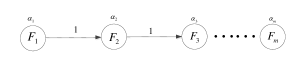
Figure 3: Graphical visualization of Case 1 with $m$ families of hypotheses.

Moreover, suppose each family has only one hypothesis, i.e., $F_{1}=\{H_{11}\},\ldots,F_{m}=\{H_{m1}\}$. Then, if the previous hypothesis is rejected, its level can be fully added to test the current one. However, if the previous hypothesis is not rejected, the current one is tested at its initially assigned level. That is, the proposed procedure reduces to the conventional fallback procedure (see Wiens, 2003; Wiens and Dmitrienko, 2005) for this case.

Case 2. Suppose retesting is involved in Case 1. The graphical representation of the new case is shown in Figure 4. According to Algorithm 2, after a round of tests for all $m$ families of hypotheses, an amount of the initial level $\alpha_{m}$ for $F_{m}$ is transferred to the local critical value of $F_{1}$ such that all $m$ families of hypotheses can have chances to be retested at the updated local critical values. Specially, if all hypotheses in $F_{m}$ are rejected, then $F_{1}$ will be retested at updated critical value $\alpha_{1}+\alpha_{m}$. Moreover, suppose each family has only one hypothesis, i.e., $F_{1}=\{H_{11}\},\ldots,F_{m}=\{H_{m1}\}$. In this case, the proposed procedure can be regarded as an improved version of the conventional fallback procedure in the sense that all $m$ hypotheses have chances to be retested at the updated critical values. For instance, if $H_{m1}$ is rejected, then $H_{11}$ can be retested at the updated level $\alpha_{1}+\alpha_{m}$.

Figure 4: Graphical visualization of Case 2 with $m$ families of hypotheses.

5 Clinical trial examples

In this section, we consider two clinical trial examples to illustrate the application of our proposed Bonferroni-based gatekeeping procedures with retesting option. The results are compared with those of our own procedures without the retesting option and the existing three procedures with retesting option, Guilbaud’s generalized Bonferroni parallel gatekeeping method with retesting (Guilbaud, 2007), Dmitrienko et al.’s $\alpha$-exhaustive multistage gatekeeping method with retesting (Dmitrienko, Kordzakhia and Tamhane, 2011) and superchain procedure (Kordzakhia and Dmitrienko, 2013). For notational convenience, the proposed procedures with and without the retesting option are labeled Retest and No-retest, and the three existing Guilbaud’s procedure, Dmitrienko et al.’s procedure and superchain procedure are labeled BR, MR and SC, respectively.

5.1 Two-family Problem

This example is based on the EPHESUS trial (see Pitt et al., 2003), in which a balanced design clinical trial is used to assess the effects of eplerenone on morbidity and mortality in patients with severe heart failure. There are two primary endpoints and two secondary endpoints grouped into two families:

• $F_{1}$: all-cause mortality (Endpoint P1) and cardiovascular mortality plus cardiovascular hospitalization (Endpoint P2).

• $F_{2}$: cardiovascular mortality (Endpoint S1) and all-cause mortality plus all-cause hospitalization (Endpoint S2).

The hypotheses of no treatment effect corresponding to these two primary endpoints and two secondary endpoints are $H_{11},H_{12}$ and $H_{21},H_{22}$, respectively. With $\alpha=0.05$, the initial levels for the two families are set at $0.04$ and $0.01$ for all aforementioned five procedures. For the proposed Retest procedure and the existing SC procedure, we used the same graphical representation as shown in Figure 5. Specifically, for the MR procedure, we applied the truncated Holm method to each family at each stage with initial truncation parameter = 0.5. For the SC procedure, we applied the Holm-based Superchain procedure. At the first step, we used Bonferroni procedure to test both families simultaneously at the initial levels. According to the testing results of the first step, we proceeded to test both families using truncated Holm procedure at updated critical values at the subsequent steps. Due to the complexity of updating rules for local critical values and truncation parameters for truncated Holm procedure, we omit the detailed steps here. For more information about updating rules of superchain procedure, see Kordzakhia and Dmitrienko (2013).

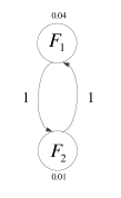
Figure 5: Graphical visualization of the two-family clinical trial problem.

The raw $p$-values for the four null hypotheses and the test results using the aforementioned three procedures are given in Table 1. The Retest procedure is implemented as follows.
Stage 1. Test null hypotheses of $F_{1}$ at level $\alpha_{1(1)}=0.04$. Since $p_{11}<\frac{0.04}{2}$ and $p_{12}>\frac{0.04}{2}$, $R_{1(1)}=\{H_{11}\}$. Hence, the level for the local critical value for $F_{2}$ is updated to

$$\alpha_{2(1)}=\alpha_{2}+\frac{1}{2}\alpha_{1(1)}=0.01+0.02=0.03.$$

Test $F_{2}$ at $\alpha_{2(1)}$. Since $p_{21}<\frac{0.03}{2}$ and $p_{22}>\frac{0.03}{2}$, $R_{2(1)}=\{H_{21}\}$. So far, the No-retest procedure stops. To proceed with the Retest procedure, we updated the level for the local critical value for $F_{1}$ to

$$\alpha_{1(2)}=\alpha_{1}+\frac{1}{2}\alpha_{2}=0.045.$$

Stage 2. Retest $F_{1}$ using the Bonferroni method at level $\alpha_{1(2)}$. Since $p_{11}<\frac{0.045}{2}$ and $p_{12}>\frac{0.045}{2}$, $R_{1(2)}=\{H_{11}\}=R_{1(1)}$. Thus, the updated level for the local critical value for $F_{2}$ is

$$\alpha_{2(2)}=\alpha_{2}+\frac{1}{2}\alpha_{1(2)}=0.0325.$$

Retest $F_{2}$ using the Bonferroni method at level $\alpha_{2(2)}$. Since $p_{21}<\frac{0.0325}{2}$ and $p_{22}<\frac{0.0325}{2}$, $R_{2(1)}=\{H_{21},H_{22}\}$. Thus, the updated level for the local critical value for $F_{1}$ is

$$\alpha_{1(3)}=\alpha_{1}+\frac{2}{2}\alpha_{2}=0.05.$$

Stage 3. Retest $F_{1}$ using the Bonferroni method at level $\alpha_{1(3)}$. Since for both $F_{1}$ and $F_{2}$, there is no new rejection, the whole Retest procedure stops.

Table 1: Comparison of the results of five procedures in the EPHESUS trial example. The initial levels for $F_{1}$ and $F_{2}$ are 0.04 and 0.01, respectively. The globe Type I error rate is $\alpha=0.05$. Note: S=significant; NS=not significant.

Family	Null	Raw	Retest	No-retest	BR	MR	SC
	hypothesis	$p$-value
$F_{1}$	$H_{11}$	0.0121	S	S	S	S	S
	$H_{12}$	0.0337	NS	NS	NS	NS	S
$F_{2}$	$H_{21}$	0.0084	S	S	S	S	S
	$H_{22}$	0.0160	S	NS	NS	NS	S

As seen from Table 1, the No-retest, BR and MR procedure only rejects two null hypotheses. but the proposed Retest rejects more, which is three. SC rejects all hypotheses. Note that for BR and MR, since not all secondary hypotheses are rejected, primary hypothses have no chance to be retested.

5.2 Three-family Problem

In this subsection, we reconsider the example disccussed in Kordzahia and Dmitrienko (2013). It is a balanced design clinical trial in which two doses (D1, D2) of a treatment are compared with a placebo (P) in the general population of patients as well as in two pre-specified subpopulations of patients. The subpopulations are defined by phenotype or genotype markers. The three populations are labeled Group 1 (General population), Group 2 (Subpopulation 1) and Group 3 (Subpopulation 2). There are six null hypotheses grouped into three families:

• $F_{1}$: $H_{11}$ (D1 vs P in Group 1) and $H_{12}$ (D2 vs P in Group 1).

• $F_{2}$: $H_{21}$ (D1 vs P in Group 2) and $H_{22}$ (D2 vs P in Group 2).

• $F_{3}$: $H_{31}$ (D1 vs P in Group 3) and $H_{32}$ (D2 vs P in Group 3).

We applied the proposed Retest, No-retest, BR, MR and SC procedures to this example. The global FWER needs to be controlled at level $\alpha=0.025$ and the initial levels for the three families were set at $\alpha_{1}=\frac{1}{2}\alpha=0.0125$, $\alpha_{2}=\frac{1}{3}\alpha=0.00833$ and $\alpha_{3}=\frac{1}{6}\alpha=0.00417$. For Retest and SC procedures, the transition matrix is pre-defined as

$$\mathbf{G}=\left(\begin{array}[]{ccc}0&0.5&0.5\\ 0.5&0&0.5\\ 0.5&0.5&0\end{array}\right).$$

Figure 6 shows its graphical representation of the three-family clinical trial example. Similar to the aforementioned two-family problem, we applied the truncated Holm procedure to each family at each stage with initial truncation parameter = 0.5 for the MR procedure. And we also applied Holm-based SC procedure to this example. As in Kordzakhia and Dmitrienko (2013), the three families are assumed to be interchangeable and can be tested in any order. At the first step, we used the Bonferroni procedure to test these three families simultaneously at their initial levels. According to the testing results at the first step, we proceeded to test the three families using the truncated Holm procedure at updated local critical values at the subsequent steps. Again, we omit the detailed steps here due to its complexity of updating rules. For more information about updating rules, see Kordzakhia and Dmitrienko (2013).

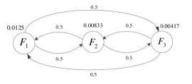
Figure 6: Graphical visualization of three-family clinical trial problem.

The raw $p$-values for six null hypotheses and the test results using the aforementioned five procedures are shown in Table 2. The proposed Retest procedure is implemented as follows.
Stage 1. Test $F_{1}$ using the Bonferroni method at level $\alpha_{1(1)}=0.0125$. Since $p_{11}>\frac{0.0125}{2}$ and $p_{12}>\frac{0.0125}{2}$, $R_{1(1)}=\emptyset$. Then, test $F_{2}$ at level $\alpha_{2(1)}=\alpha_{2}=0.00833$. Since $p_{21}>\frac{0.00833}{2}$ and $p_{22}>\frac{0.00833}{2}$, $R_{2(1)}=\emptyset$. Test $F_{3}$ at level $\alpha_{3(1)}=\alpha_{3}=0.00417$. Since $p_{31}>\frac{0.00417}{2}$ and $p_{32}<\frac{0.00417}{2}$, $R_{3(1)}=\{H_{32}\}$. The No-retest procedure stops here. The proposed Retest procedure proceeds to the next stage.
Stage 2. Retest $F_{1}$ using the Bonferroni method at level

$$\alpha_{1(2)}=\alpha_{1}+\frac{1}{2}g_{31}\alpha_{3}=0.0125+\frac{1}{2}\cdot 0.5\cdot 0.00417=0.0135.$$

Since $p_{11}>\frac{0.00135}{2}$ and $p_{12}>\frac{0.0135}{2}$, $R_{2(1)}=\emptyset$. Then retest $F_{2}$ at level

$$\alpha_{2(2)}=\alpha_{2}+\frac{1}{2}g_{32}\alpha_{3}=0.00833+\frac{1}{2}\cdot 0.5\cdot 0.00417=0.00937.$$

Since $p_{21}>\frac{0.00937}{2}$ and $p_{22}<\frac{0.00937}{2}$, $R_{2(2)}=\{H_{22}\}$. Retest $F_{3}$ at level

$$\alpha_{3(2)}=\alpha_{3}+g_{23}\alpha_{2(2)}=0.00417+\frac{1}{2}\cdot 0.5\cdot 0.00937=0.0065.$$

Since $p_{31}>\frac{0.0065}{2}$ and $p_{32}<\frac{0.0065}{2}$, $R_{3(2)}=\{H_{32}\}$. Thus, there are no new rejections in $F_{3}$ at this stage and hence the testing algorithm stops. The final set of rejected null hypotheses is $\{H_{22},H_{32}\}$.

Table 2: Comparison of results of three procedures in the dose-response trial example. The initial critical values for $F_{1}$, $F_{2}$ and $F_{3}$ are 0.0125, 0.00833 and 0.00417, respectively. The globe Type I error rate is $\alpha=0.025$. Note: S=significant; NS=not significant.

Family	Null	Raw	Retest	No-retest	BR	MR	SC
	hypothesis	$p$-value
$F_{1}$	$H_{11}$	0.0092	NS	NS	NS	NS	NS
	$H_{12}$	0.0105	NS	NS	NS	NS	NS
$F_{2}$	$H_{21}$	0.0059	NS	NS	NS	NS	NS
	$H_{22}$	0.0044	S	NS	NS	NS	S
$F_{3}$	$H_{31}$	0.0271	NS	NS	NS	NS	NS
	$H_{32}$	0.0013	S	S	S	S	S

As seen from Table 2, the No-retest, BR and MR procedure has poor performance. It only rejects $H_{32}$. By contrast, the proposed Retest and Holm-based SC procedures reject $H_{32}$ as well as $H_{22}$.

Remark 7

These two examples illustrate that our proposed Retest procedure has power improvement over No-retest procedure and BR procedure. In many cases, it performs better than MR procedure and is comparable with the Holm-based SC procedure in terms of power. For BR procudure, although one higher rank family is possible to be retested by a method more powerful than Bonferroni method, it can be retested only if all of the hypotheses in lower rank families are rejected. For MR procedure, although it is based on the method which is more powerful than Bonferroni method (i.e., truncated version of multiple testing procedures) at each stage, it will stop testing early if there are many acceptances occurs in the higher rank families. Since only a small amount of critical value can be carried over to test subsequent families. Moreover, the common problem for both BR and MR procedure is that since the retesting order is from last family to first family, the higher rank important families will have less chance to be retesd than lower-rank families which is counterintuitive in the sense of hierarchical sequential testing. Compared with the proposed procedure, the implementation of the SC procedure is complicated due to its complex updating rules of the local critical values and truncation parameters at each stage, especially when the number of families is large.

6 An Extension

In the preceding sections, we considered only one family within each layer while testing hierarchically ordered families of hypotheses. However, there are situations where there are multiple families within a layer. For instance, in clinical trials where both multiple primary and multiple secondary endpoints are evaluated in several patient populations, each family of hypotheses corresponds to one primary or secondary endpoint and the families corresponding to all the primary endpoints and the secondary endpoints are grouped as primary layer and secondary layer, respectively.

In this section, we consider a complex two-layer hierarchical structure with multiple families of hypotheses within each layer. Using similar idea as in developing Algorithm 2, we develop a procedure with retesting option in which the families between layers are tested sequentially while those within each layer are tested simultaneously. Each family is still allowed to be iteratively retested using the Bonferroni procedure with repeatedly updated local critical values. The procedure is designed to strongly control the global FWER at $\alpha$ under arbitrary dependence.

Suppose that $n\geq 2$ hypotheses are grouped into $m\geq 2$ families which are divided into two layers, with $F_{i1},\ldots,F_{im_{i}}$ being the families of the $i$th layer, for $i=1,2$, where $\sum_{i=1}^{2}m_{i}=m$. Let the family $F_{ij}$ have $n_{ij}\geq 1$ null hypotheses, where $\sum_{i=1}^{2}\sum_{j=1}^{m_{i}}n_{ij}=n$. For $i=1,2;j=1,\ldots,m_{i}$, let $\alpha_{ij}$ denote the initial critical value assigned to $F_{ij}$ such that $\sum_{i=1}^{2}\sum_{j=1}^{m_{i}}\alpha_{ij}=\alpha$. The distribution of critical values transferred among families can be pre-fixed by a transition coefficient set which is defined as follows.

Denote $\mathbf{G}$ = {$g_{ijkl}$}, $i,k=1,2,j=1,\ldots,m_{i},l=1,\ldots,m_{k}$ as a set of transition coefficients satisfying the following conditions:

$$0\leq g_{ijkl}\leq 1;\>\>g_{ijkl}=0,\text{ if }i=k;$$

$$\sum_{l=1}^{m_{2}}g_{1j2l}=1,\text{ for any }j=1,\ldots,m_{1};\>\>\sum_{j=1}^{m_{1}}g_{2l1j}=1,\text{ for any }l=1,\ldots,m_{2}.$$

The $g_{ijkl}$ is used to determine the proportion of the level associated with $F_{ij}$ that can be transferred to $F_{kl}$. Figure 7 shows the graphical representation of the case of two layers with four families.

Figure 7: Two-layer with four families Bonferroni - based gatekeeping procedure with retesting option.

The proposed procedure allows all $m$ families of hypotheses to be tested more than once. For notational conveniences, let the local critical value used to test $F_{ij}$ for the $t^{th}$ time be $\alpha_{ij_{(t)}}$. Let $R_{{ij}_{(t)}}$ be the set of rejected hypotheses when $F_{ij}$ is tested for the $t^{th}$ time with the cardinality $|R_{{ij}_{(t)}}|$. The algorithm for the two-layer Bonferroni-based gatekeeping procedure with retesting option is as follows.

Algorithm 3

Stage 1. Test $F_{1j},j=1,\ldots,m_{1}$ simultaneously using the Bonferroni method at level $\alpha_{1j_{(1)}}=\alpha_{1j}$. Update the local critical values for $F_{2l},l=1,\ldots,m_{2}$ to

$$\alpha_{2l_{(1)}}=\alpha_{2l}+\sum_{j=1}^{m_{1}}\frac{|R_{1j_{(1)}}|}{n_{1j}}g_{1j2l}\alpha_{1j}.$$

Test $F_{2l},l=1,\ldots,m_{2}$ simultaneously at level $\alpha_{2l_{(1)}}$ using the Bonferroni method. If no hypotheses are rejected among all $m$ families, the algorithm stops. Otherwise, it continues to the next stage.
Stage $\bm{k(k\geq 2)}$. For $j=1,\ldots,m_{1}$, set

$$\alpha_{1j_{(k)}}=\alpha_{1j}+\sum_{l=1}^{m_{2}}\frac{|R_{2l_{(k-1)}}|}{n_{2l}}g_{2l1j}\alpha_{2l}.$$ (5)

Retest $F_{1j},j=1,\ldots,m_{1}$ simultaneously at level $\alpha_{ij_{(k)}}$ using the Bonferroni method and update the local critical values for $F_{2l},l=1,\ldots,m_{2}$ to

$$\alpha_{2l_{(k)}}=\alpha_{2l}+\sum_{j=1}^{m_{1}}\frac{|R_{1j_{(k)}}|}{n_{1j}}g_{1j2l}\alpha_{1j_{(k)}}.$$

Retest $F_{2l},l=1,\ldots,m_{2}$, simultaneously at level $\alpha_{2l_{(k)}}$ using the Bonferroni method. If no new null hypotheses are rejected among all $m$ families, the algorithm stops. Otherwise, it continues to the next stage.

Remark 8

In Algorithm 3, the families of hypotheses within a layer are tested simultaneously, however, the families across layers are tested in a sequential manner. For each family, its local critical value is updated on the basis of the results of the most recent tests of families within other layer. It is seen from Algorithm 3 that with increasing number of retesting stages, the updated local critical value of each family is non-decreasing, which in turn implies its number of rejection is also non-decreasing. Besides, when more rejections occur in one family, larger portions of its local critical value are transferred to the families within other layer. When all families of one layer have no new hypotheses rejected, the whole algorithm stops.

Remark 9

Consider the problem of two layers with four families as described in Figure 7. Regarding Algorithm 3 and relevant scenarios, we have the following observations:

1. Suppose $\alpha_{12}=\alpha_{22}=0$ and $g_{1121}=g_{2111}=1$. Then, each layer only has one family of hypotheses. Thus, Algorithm 3 reduces to Algorithm 1 introduced in Section 3.1.

2. Suppose $g_{1122}=g_{2211}=g_{1221}=g_{2112}=0$. Then, each family of the first layer is only related to one specific family of the second layer, that is, the hierarchical logical relationships among families are given in advance. In this case, the proposed Algorithm 3 takes into account such hierarchical logical relationships.

3. Suppose $\alpha_{12}=0$ and $g_{1221}=g_{1222}=g_{2112}=g_{2212}=0$. Then, both families of the second layer only rely on the testing results of one particular family of the first layer. Thus, we can regard it as the case that both “child” families share one “parent” family, which is similar to a tree structure with retesting option. Moreover, suppose $\alpha_{12}=0$ but $g_{2112}\neq 0$ and $g_{2212}\neq 0$. Then, $F_{12}$ still has a chance to be tested at the retesting stages due to the portions of levels transferred from the “child” families of the second layer.

4. Suppose $\alpha_{22}=0$, then the testing results of two families of the first layer can both contribute to the local critical value of the first family of the second layer. Thus, we can regard it as the case that one “child” family has two “parent” families.

For algorithm 3, we have the following theorem.

Theorem 2

The two-layer Bonferroni-based gatekeeping procedure with retesting option described in Algorithm 3 strongly controls the global FWER at level $\alpha$ under arbitrary dependence.

For a proof of Theorem 2, see appendix.

7 Concluding Remarks

The main focus of this paper has been to develop simple and powerful procedures for testing ordered families of hypotheses. We have introduced a new multiple testing procedure, termed as Bonferroni-based gatekeeping procedure with retesting option, in which the families of hypotheses are repeatedly tested by the Bonferroni procedure at updated local critical values in a sequential manner. We have shown that the proposed procedure strongly controls the global FWER at level $\alpha$ under arbitrary dependence. Through two clinical trial examples, we have illustrated the straightforward testing algorithm of our proposed procedure.

Both Guibaud’s generalized Bonferroni parallel gatekeeping procedure and our proposed procedure are based on simple Bonferroni method. But Guibaud’s procedure requires rejecting all hypotheses in the last family to start retesting. Although Dmiritneko et al.’s $\alpha$-exhaustive multistage gatekeeping procedure improves Guibaud’s procedure by using more powerful method than Bonferroni method to test each family, the common counterintuitive problem with Guibaud’s method that lower rank families having more chances to be retested than higher rank families still exists.

Both the superchain procedure and our proposed procedure allow iteratively retesting families of hypotheses and both of them have power improvement compared with the procedure without retesting option. Although by choosing the optimized initial parameters and initial multiple testing procedure for each family, the superchain procedure might has its advantage over our procedure with respect to power, however, the proposed procedure has some better, desirable features.

While trying to solve problems associated with testing multiple ordered families of hypotheses in real life applications, it is desirable to have simplicity in the testing procedures. Our proposed procedure enjoys that simplicity when compared with the superchain procedure. The sequential testing strategy in our proposed procedure seems more natural than the superchain procedure which tests all families simultaneously. Given the families to be tested, the transition matrix, and the initial critical values, our procedure can be easily implemented as a graphical form based on the simple Bonferroni procedure. No matter how many iterations each family has been through, the testing procedure used at each stage for each family never changes. On the contrary, for the superchain procedure, even the graph of families is given, the specific algorithm cannot be defined. One graph may have different superchain algorithms which leads to completely different testing results. It has been mentioned by Kordzakhia and Dmitrienko (2013) that the performance of the superchain procedure heavily depends on the choices of initial parameters, i.e., the initial truncation parameters, and the initial local method. They have shown that the power of the superchain procedures can dramatically differ with changing initial values of the truncated parameters. Thus, before starting to implement the superchain procedure, we first need to make some efforts to decide the optimal values of initial procedure parameters which add more complexities into the implementation.

From the computational point of view, our procedure is simple and easy to implement. The implementation of the superchain procedure is complicated due to the updating rules of the local critical values and the truncation parameters of the testing procedure for each family at each stage. The computational complexity is even more severe when the number of families is large. Because of these, it is difficult to communicate with non-statisticians about the algorithm of the superchain procedure.

The use of the Bonferroni procedure as the basic procedure for testing each family makes our proposed procedure slightly conservative compared to the Dimitrienko et al.’s $\alpha$-exhaustive multistage gatekeeping procedure and superchain procedure in some cases. Therefore, a natural extension of our present work would be to use more powerful multiple testing procedures as the basic procedures toward developing a more powerful global FWER controlling sequential procedures with retesting option. In addition, the proposed procedure controls the global FWER without any assumption of dependence structure among the underlying test statistics. Given some distributional information about the test statistics, it is possible to further improve the proposed procedure.

Appendix

Proof of Theorem 1

Let $V_{k}$ be the total number of false rejections among all $m$ families of hypotheses in the first $k$ stages by using the Bonferroni-based gatekeeping procedure with retesting option. Denote $\text{FWER}_{k}$ as the FWER of this procedure in the first $k$ stages such that $\text{FWER}_{k}=\text{Pr}(V_{k}\geq 1)$. Therefore, the global FWER of this procedure is $\text{FWER}=\text{Pr}\left(\cup_{k=1}^{\infty}\left\{V_{k}\geq 1\right\}\right)$. Let $D_{j}$ denote the event that at least one true null hypotheses is rejected among all $m$ families at stage $j$, $E_{i(j)}$ denote the event that at least one true null hypothesis is rejected in $F_{i}$ at stage $j$, and $\overline{E}_{i(j)}$ denote the complement of $E_{i(j)}$. Thus, $\left\{V_{k}\geq 1\right\}=\cup_{j=1}^{k}D_{j}$ and $D_{j}=\bigcup_{i=1}^{m}E_{i(j)}$. Then, we have

$$\text{FWER}_{k} = \text{Pr}(V_{k}\geq 1)=\text{Pr}\left\{\cup_{j=1}^{k}D_{j}\right\}.$$

Thus,

$$1-\text{FWER}_{k} = \text{Pr}\left(\overline{D}_{k}\cap\left\{\cap_{j=1}^{k-1}\overline{D}_{j}\right\}\right)$$ (6)

$$= \text{Pr}\left(\cap_{j=1}^{k-1}\overline{D}_{j}|\overline{D}_{k}\right)\text{Pr}\left(\overline{D}_{k}\right)$$

$$= \text{Pr}\left(\overline{D}_{k}\right),$$

where the second equality follows from the fact that any family at stage $k$ is tested with a more powerful test than the test used in the first $k-1$ stages. Thus, if no true null hypotheses are rejected in any family at stage $k$, then no true nulls are rejected in the first $k-1$ stages with probability 1.

By (6), in order to show $\text{FWER}_{k}\leq\alpha$, it is sufficient to show

$$1-\text{Pr}\left(\overline{D}_{k}\right)\leq\alpha.$$

Let $p_{ij},i=1,\ldots,m,j=1,\ldots,n_{i}$ denote the $p$-value corresponding to the null hypothesis $H_{ij}$ in family $F_{i}$. Define $T_{i}$ the set of true null hypotheses within $F_{i}$ with the cardinality $|T_{i}|,i=1,\ldots,m$. Then

$$\text{Pr}\left(\overline{D}_{k}\right) = \text{Pr}\left(\bigcap_{i=1}^{m}\overline{E}_{i(k)}\right)$$ (7)

$$\geq \text{Pr}\left\{\bigcap_{i=1}^{m}\bigcap_{H_{ij}\in T_{i}}\left\{p_{ij}>\frac{\alpha_{i(k)}^{*}}{n_{i}}\right\}\right\},$$

where

$$\alpha_{1(k)}^{*}=\alpha_{1}+\sum_{l=2}^{m}\left(1-\frac{|T_{l}|}{n_{l}}\right)g_{l1}\alpha_{l}$$ (8)

and

$$\alpha_{i(k)}^{*}=\alpha_{i}+\sum_{j=1}^{i-1}\left(1-\frac{|T_{j}|}{n_{j}}\right)g_{ji}\alpha_{j(k)}+\sum_{l=i+1}^{m}\left(1-\frac{|T_{l}|}{n_{l}}\right)g_{li}\alpha_{l},$$ (9)

for $i=2,\ldots,m$. Here, the inequality (7) follows from the argument that when the event $\overline{D}_{k}$ occurs, no true null hypotheses are rejected among all $m$ families at stage $k$, which in turn implies that no true null hypotheses are rejected in the first $k-1$ stages. Thus, $|R_{j(k-1)}|\leq|R_{j(k)}|\leq n_{j}-|T_{j}|$ for $j=1,\ldots,m$. By comparing (9) with (4), we have $\alpha_{i(k)}\leq\alpha_{i(k)}^{*}$ for $i=1,\ldots,m$, and then (7) follows.

In order to prove the $\text{FWER}_{k}$ control, we need to use the following lemma.

Lemma 1

Consider a function $f$ defined by

$$f(j) = \sum_{i=1}^{j}\left[\frac{|T_{i}|}{n_{i}}+\left(1-\frac{|T_{i}|}{n_{i}}\right)\left(\sum_{l=j+1}^{m}g_{il}\right)\right]\alpha_{i(k)}^{*}$$

$$+\sum_{l=j+1}^{m}\left[\frac{|T_{l}|}{n_{l}}+\left(1-\frac{|T_{l}|}{n_{l}}\right)\left(\sum_{i=j+1}^{m}g_{li}\right)\right]\alpha_{l}$$

on the set $\{2,\ldots,m-1\}$. The function $f(j)$ is non-increasing in terms of $j$.

Proof of Lemma 1 To show $f(j)$ is a non-increasing function on $j=2,\ldots,m-1$, it is sufficient to show that $f(j)\leq f(j-1)$ for any $j=3,\ldots,m-1$. Note that

$$\quad f(j) = \sum_{i=1}^{j-1}\left[\frac{|T_{i}|}{n_{i}}+\left(1-\frac{|T_{i}|}{n_{i}}\right)\left(\sum_{l=j+1}^{m}g_{il}\right)\right]\alpha_{i(k)}^{*}$$

$$\quad+\sum_{l=j+1}^{m}\left[\frac{|T_{l}|}{n_{l}}+\left(1-\frac{|T_{l}|}{n_{l}}\right)\left(\sum_{i=j+1}^{m}g_{li}\right)\right]\alpha_{l}$$

$$\quad+\left[\frac{|T_{j}|}{n_{j}}+\left(1-\frac{|T_{j}|}{n_{j}}\right)\left(\sum_{i=j+1}^{m}g_{ji}\right)\right]\alpha_{j(k)}^{*}$$

$$\leq \sum_{i=1}^{j-1}\left[\frac{|T_{i}|}{n_{i}}+\left(1-\frac{|T_{i}|}{n_{i}}\right)\left(\sum_{l=j+1}^{m}g_{il}\right)\right]\alpha_{i(k)}^{*}$$

$$\quad+\sum_{l=j+1}^{m}\left[\frac{|T_{l}|}{n_{l}}+\left(1-\frac{|T_{l}|}{n_{l}}\right)\left(\sum_{i=j+1}^{m}g_{li}\right)\right]\alpha_{l}$$

$$\quad+\left[\frac{|T_{j}|}{n_{j}}+\left(1-\frac{|T_{j}|}{n_{j}}\right)\left(\sum_{i=j+1}^{m}g_{ji}\right)\right]\alpha_{j}$$

$$\quad+\sum_{i=1}^{j-1}\left(1-\frac{|T_{i}|}{n_{i}}\right)g_{ij}\alpha^{*}_{i(k)}+\sum_{l=j+1}^{m}\left(1-\frac{|T_{l}|}{n_{l}}\right)g_{lj}\alpha_{l}$$

$$= \sum_{i=1}^{j-1}\left[\frac{|T_{i}|}{n_{i}}+\left(1-\frac{|T_{i}|}{n_{i}}\right)\left(\sum_{l=j}^{m}g_{il}\right)\right]\alpha_{i(k)}^{*}$$

$$\quad+\sum_{l=j}^{m}\left[\frac{|T_{l}|}{n_{l}}+\left(1-\frac{|T_{l}|}{n_{l}}\right)\left(\sum_{i=j}^{m}g_{li}\right)\right]\alpha_{l}$$

$$= f(j-1),$$

the desired result follows. $\square$ By (7), we note that

$$1-\text{Pr}\left(\overline{D}_{k}\right)$$ (11)

$$\leq \sum_{i=1}^{m}\text{Pr}\left\{\bigcup_{H_{ij}\in T_{i}}\left\{\hat{p}_{ij}~{}~{}\leq\quad\frac{\alpha_{i(k)}^{*}}{n_{i}}\right\}\right\}\leq\sum_{i=1}^{m}\frac{|T_{i}|}{n_{i}}\alpha_{i(k)}^{*}$$

$$= \sum_{i=1}^{m-1}\frac{|T_{i}|}{n_{i}}\alpha_{i(k)}^{*}+\frac{|T_{m}|}{n_{m}}\left[\alpha_{m}+\sum_{i=1}^{m-1}\left(1-\frac{|T_{i}|}{n_{i}}\right)g_{im}\alpha_{i(k)}^{*}\right]$$

$$= \sum_{i=1}^{m-1}\left[\frac{|T_{i}|}{n_{i}}+\left(1-\frac{|T_{i}|}{n_{i}}\right)g_{im}\right]\alpha_{i(k)}^{*}+\frac{|T_{m}|}{n_{m}}\alpha_{m}$$

$$\leq \left[\frac{|T_{1}|}{n_{1}}+\left(1-\frac{|T_{1}|}{n_{1}}\right)\left(\sum_{l=2}^{m}g_{1l}\right)\right]\alpha_{1(k)}^{*}$$

$$\quad+\sum_{l=2}^{m}\left[\frac{|T_{l}|}{n_{l}}+\left(1-\frac{|T_{l}|}{n_{l}}\right)\left(\sum_{j=2}^{m}g_{lj}\right)\right]\alpha_{l}$$

$$= \alpha_{1(k)}^{*}+\sum_{l=2}^{m}\left[\frac{|T_{l}|}{n_{l}}+\left(1-\frac{|T_{l}|}{n_{l}}\right)\left(\sum_{j=2}^{m}g_{lj}\right)\right]\alpha_{l}$$ (12)

$$= \alpha_{1}+\sum_{l=2}^{m}\left[\frac{|T_{l}|}{n_{l}}+\left(1-\frac{|T_{l}|}{n_{l}}\right)\left(\sum_{j=1}^{m}g_{lj}\right)\right]\alpha_{l}$$

$$= \sum_{l=1}^{m}\alpha_{l}=\alpha,$$

where (11) holds due to the fact that $\alpha_{i(k)}^{*}$ is not random for any $i=1,\ldots,m$ and the $U(0,1)$ assumption of true null $p$-values. The inequality (11) holds due to Lemma 1 and the equalities (12) and (Proof of Theorem 1) hold due to the transition matrix condition that for any $i=1,\ldots,m$, $\sum_{j=1}^{m}g_{ij}=1$ and $g_{ii}=0$. Thus, by (6), we have that for any $k$,

$$\text{FWER}_{k}=1-\text{Pr}\left(\overline{D}_{k}\right)\leq\alpha.$$ (14)

Since $V_{k}$ is non-decreasing in $k$, the events $\{V_{k}\geq 1\}_{k\geq 1}$ is an increasing sequence of events. Then

$$\text{FWER}=\text{Pr}(\cup_{k=1}^{\infty}\{V_{k}\geq 1\})$$ (15)

$$= \lim_{k\rightarrow\infty}\text{Pr}\left(V_{k}\geq 1\right)=\lim_{k\rightarrow\infty}\text{FWER}_{k}\leq\alpha,$$

the desired result. $\square$

Proof of Theorem 2

Using the same notations $V_{k}$, $D_{k}$ and $\text{FWER}_{k}$ as in the proof of Theorem 1, the global FWER of the two-layer Bonferroni-based gatekeeping procedure with retesting option is still expressed as $\text{FWER}=\text{Pr}\left(\cup_{k=1}^{\infty}\left\{V_{k}\geq 1\right\}\right)$. By using the same argument as in the proof of (6), we have

$$\text{FWER}_{k}=\text{Pr}\left(V_{k}\geq 1\right)=1-\text{Pr}\left(\overline{D}_{k}\right).$$

To show $\text{FWER}_{k}\leq\alpha$, it is enough to show

$$1-\text{Pr}\left(\overline{D}_{k}\right)\leq\alpha.$$

Let $p_{ijs}$ denote the $p$-value corresponding to the null hypothesis $H_{ijs}$ in family $F_{ij}$, $i=1,2,j=1,\ldots,m_{i}$ and $s=1,\ldots,n_{ij}$. Define $T_{ij}$ the set of true null hypotheses within $F_{ij}$ with the cardinality $|T_{ij}|$. By using the same argument as in the proof of (7), we have

$$\text{Pr}\left(\overline{D}_{k}\right)\geq\text{Pr}\left(\left\{\bigcap_{j=1}^{m_{1}}\bigcap_{H_{1js}\in T_{1j}}\left\{p_{1js}>\frac{\alpha_{1j_{(k)}}^{*}}{n_{1j}}\right\}\right\}\bigcap\left\{\bigcap_{l=1}^{m_{2}}\bigcap_{H_{2ls}\in T_{2l}}\left\{p_{2ls}>\frac{\alpha_{2l_{(k)}}^{*}}{n_{2l}}\right\}\right\}\right),$$

where

$$\alpha_{1j_{(k)}}^{*}=\alpha_{1j}+\sum_{l=1}^{m_{2}}\left(1-\frac{|T_{2l}|}{n_{2l}}\right)g_{2l1j}\alpha_{2l},$$

$$\alpha_{2l_{(k)}}^{*}=\alpha_{2l}+\sum_{j=1}^{m_{1}}\left(1-\frac{|T_{1j}|}{n_{1j}}\right)g_{1j2l}\alpha_{1j_{(k)}}^{*}.$$

Thus,

$$1-\text{Pr}\left(\overline{D}_{k}\right) \leq \sum_{j=1}^{m_{1}}\text{Pr}\left\{\bigcup_{H_{1js}\in T_{1j}}\left\{{p}_{1js}\leq\frac{\alpha_{1j_{(k)}}^{*}}{n_{1j}}\right\}\right\}$$

$$\quad+\sum_{l=1}^{m_{2}}\text{Pr}\left\{\bigcup_{H_{2ls}\in T_{2l}}\left\{{p}_{2ls}\leq\frac{\alpha_{2l_{(k)}}^{*}}{n_{2l}}\right\}\right\}$$

$$\leq \sum_{j=1}^{m_{1}}\frac{|T_{1j}|}{n_{1j}}\alpha_{1j_{(k)}}^{*}+\sum_{l=1}^{m_{2}}\frac{|T_{2l}|}{n_{2l}}\left[\alpha_{2l}+\sum_{j=1}^{m_{1}}\left(1-\frac{|T_{1j}|}{n_{1j}}\right)g_{1j2l}\alpha_{1j_{(k)}}^{*}\right]$$

$$= \sum_{j=1}^{m_{1}}\left[\alpha_{1j}+\sum_{l=1}^{m_{2}}\left(1-\frac{|T_{2l}|}{n_{2l}}\right)g_{2l1j}\alpha_{2l}\right]+\sum_{l=1}^{m_{2}}\frac{|T_{2l}|}{n_{2l}}\alpha_{2l}$$

$$= \sum_{j=1}^{m_{1}}\alpha_{1j}+\sum_{l=1}^{m_{2}}\left(1-\frac{|T_{2l}|}{n_{2l}}\right)\alpha_{2l}+\sum_{l=1}^{m_{2}}\frac{|T_{2l}|}{n_{2l}}\alpha_{2l}$$

$$= \sum_{j=1}^{m_{1}}\alpha_{1j}+\sum_{l=1}^{m_{2}}\alpha_{2l}=\alpha.$$

The first inequality follows from Bonferroni’s inequality and the second follows from the assumption that true null $p$-values follow $U(0,1)$. The first and second equalities hold due to the conditions of the transition coefficient set. Therefore, we have

$$\text{FWER}_{k}=1-\text{Pr}\left(\overline{D}_{k}\right)\leq\alpha.$$ (16)

By using the same argument as in the proof of (15), we have

$$\text{FWER}=\lim_{k\rightarrow\infty}\text{FWER}_{k}\leq\alpha,$$

the desired result. $\square$

References

- [1]
- [2] Alosh M., Bretz F. and Huque M. (2014). Advanced multiplicity adjustment methods in clinical trials. Statistics in Medicine 33, 693–713.
- [3] Bauer P., Rohmel J., Maurer W. and Hothorn L. (1998). Testing strategies in multi-dose experiments including active control. Statistics in Medicine 17, 2133–2146.
- [4] Bretz F., Maurer W., Brannath W. and Posch M. (2009). A graphical approach to sequentially rejective multiple test procedures. Statistics in Medicine 28, 586–604.
- [5] Burman C. F., Sonesson C. and Guilbaud O. (2009). A recycling framework for the construction of Bonferroni-based multiple tests. Statistics in Medicine 28, 739–761.
- [6] Chen X., Luo X. and Capizzi T. (2005). The application of enhanced parallel gatekeeping strategies. Statistics in Medicine 24, 1385–1397.
- [7] Dmitrienko A., D’Agostino R. B. and Huque M. F. (2013). Key multiplicity issues in clinical drug development. Statistics in Medicine 32, 1079–1111.
- [8] Dmitrienko A., Kordzakhia G. and Tamhane A. C. (2011). Multistage and mixture gatekeeping procedures in clinical trials. Journal of Biopharmaceutical Statistics 21, 726–747.
- [9] Dmitrienko A., Millen B. A., Brechenmacher T. and Paux G. (2011). Development of gatekeeping strategies in confirmatory clinical trials. Biometrical Journal 53, 875–893.
- [10] Dmitrienko A., Offen W. and Westfall P. H. (2003). Gatekeeping strategies for clinical trials that do not require all primary effects to be significant. Statistics in Medicine 22, 2387–2400.
- [11] Dmitrienko A. and Tamhane A. C. (2011). Mixtures of multiple testing procedures for gatekeeping applications in clinical trials. Statistics in Medicine 30, 1473–1488.
- [12] Dmitrienko A., Tamhane A. C. and Bretz F. (2009). Gatekeeping procedures in clinical trials. In Multiple Testing Problems in Pharmaceutical Statistics, Chapter 5. Chapman and Hall/CRC Press: New York, 2009.
- [13] Dmitrienko A., Tamhane A. C., Liu L. and Wiens B. L. (2008). A note on tree gatekeeping procedures in clinical trials. Statistics in Medicine 27, 3446–3451.
- [14] Dmitrienko A., Tamhane A. C., Wang X. and Chen X. (2006). Stepwise gatekeeping procedures in clinical trial applications. Biometrical Journal 48, 984–991.
- [15] Dmitrienko A., Tamhane A. C. and Wiens B. L. (2008). General multistage gatekeeping procedures. Biometrical Journal 50, 667–677.
- [16] Dmitrienko A., Wiens B. L. and Tamhane A. C. (2007). Tree–structured gatekeeping tests in clinical trials with hierarchically ordered multiple objectives. Statistics in Medicine 26, 2465–2478.
- [17] Guilbaud O. (2007). Bonferroni parallel gatekeeping - transparent generalizations, adjusted p-values, and short direct proofs. Biometrical Journal 49, 917–927.
- [18] Kim H., Entsuah A. R. and Shults J. (2011). The union closure method for testing a fixed sequence of families of hypotheses. Biometrika 98, 391–401.
- [19] Kordzakhia G. and Dmitrienko A. (2013). Superchain procedures in clinical trials with multiple objectives. Statistics in Medicine 32, 486–508.
- [20] Liu Y. and Hsu J. (2009). Testing for efficacy in primary and secondary endpoints by partitioning decision paths. Journal of the American Statistical Association 104, 1661–1670.
- [21] Maurer W., Hothorn L. and Lehmacher W. (1995). Multiple comparisons in drug clinical trials and preclinical assays: a-priori ordered hypotheses. In Biometrie in der Chemisch-pharmazeutischen Industrie, Vollmar J(ed.). Fischer Verlag: Stuttgart, 6, 3–18.
- [22] Pitt B., Remme W., Zannad F., Neaton J., Martinez F., Roniker B., Bittman R., Hurley S., Kleiman J. and Gatlin M. (2003). Eplerenone, a selective aldosterone blocker, in patients with left ventricular dysfunction after myocardial infarction. New England Journal of Medicine 348, 1309–1321.
- [23] Westfall P. H. and Krishen A. (2001). Optimally weighted, fixed-sequence, and gatekeeping multiple testing procedures. Journal of Statistical Planning and Inference 99, 25–40.
- [24] Wiens B. L. (2003). A fixed-sequence Bonferroni procedure for testing multiple endpoints. Pharmaceutical Statistics 2, 211–215.
- [25] Wiens B. L. and Dmitrienko A. (2005). The fallback procedure for evaluating a single family of hypotheses. Journal of Biopharmaceutical Statistics 15, 929–942.
- [26]