Extracting information from random data. Applications of laws of large numbers in technical sciences and statistics.

Abstract.

We formulate conditions for convergence of Laws of Large Numbers and show its links with of the parts of mathematical analysis such as summation theory, convergence of orthogonal series. We present also applications of the Law of Large Numbers such as Stochastic Approximation, Density and Regression Estimation, Identification.

Acknowledgement 1.

The author would like to thank two of his students and co-workers dr. dr. Marcin Dudziński and Wojciech Matysiak for correction of the manuscript.

List of symbols and denotations

$x$, $y$, $\ldots$, $\alpha$, $\beta$, $\ldots-$ real numbers,

$\mathbf{x}$, $\mathbf{y}$, $\ldots$ -vectors, always column

$\mathbf{A}$, $\mathbf{B}$, $\ldots$ -matrices,

$\mathbf{x}^{T}$, $\mathbf{A}^{T},\ldots$ -transposition of vector, matrix

$A$, $B$, $\ldots$ -events, subsets of some space of elementary events $\Omega$,

$A^{c}$, $\bar{A}$ -composition of event $A,$

$A\cap B$, $A\cup B$, $A\vartriangle B$ respectively product, union and the symmetric difference of two sets $A$ and $B,$

$\omega$ element of the space of elementary events - elementary event, $\omega\in\Omega$

$P(A)$ -probability of an event $A,$

$I(A)(\omega)=\left\{\begin{array}[c]{ccc}1,&if&\omega\in A\\ 0,&if&\omega\notin A\end{array}\right.$ -indicator function of the event $A$, often denoted simply by $I(A),$

$X$, $Y$, $Z$, $\ldots$ -random variables,

$\mathbf{X,Y,\ldots}$ -random vectors,

$EX$, $EY$, $\ldots$ -expectations of the random variables,

$\sigma(X),\sigma(\mathbf{Y),}\sigma(X,Y,Z)$ -$\sigma-$ fields generated respectively by the random variable $X$, random vector $\mathbf{Y}$, random variables $X,Y,Z,$

$\mathcal{A}$, $\mathcal{B},\mathcal{C}$, $\ldots$ -denotations of $\sigma-$ fields,

$E(X|\mathcal{F})$ -conditional expectation with respect to the $\sigma-$ field $\mathcal{F},$

$P(A|\mathcal{G)}$ -conditional probability with respect to the $\sigma-$ field $\mathcal{G},$

$\left\{x_{i}\right\}_{i\geq 1}$, $\left\{Y_{i}\right\}_{i\geq 0}$, $\left\{A_{i}\right\}_{i\geq 2}$ -sequences respectively, of real numbers, random variables, events,

$\mathbb{N},\mathbb{R},\mathbb{Z},\mathbb{C}$ –sets respectively, of natural numbers, real numbers, integers and complex numbers,

$\#A$ -cardinality of the set $A,$

$\left|A\right|$ - Lebesgue measure of the set $A.$

$\left\{X<x\right\}$, $\left\{\sum X_{i}\;\text{converges }\right\}$ -shortened denotation of the events $\left\{\omega:X(\omega)<x\right\}$,
$\left\{\omega:\sum X_{i}(\omega)\;\text{converges}\right\},$

$x^{+}=\left\{\begin{array}[c]{ccc}x&if&x\geq 0\\ 0&if&x<0\end{array}\right.$ -other words positive part of $x.$

a.e., a.s. - respectively almost everywhere, almost surely. Refers to events that have zero measures or probabilities.

Preface

By iterative we mean those random phenomena that can be presented in the following form:

Next observation = function of (the present observation) + correction,

  

It means that the information based on the knowledge collected so far, complemented by the actually observed ”correction” is the base of the knowledge about the future behavior of the examined random phenomenon.

A typical example of such ”iterative” approach is the so-called law of large numbers, or behavior of the averages of observed measurements. More precisely, if the measured quantities are denoted by $x_{i}$, $i=\allowbreak 1,\allowbreak 2,\allowbreak\ldots$, then their averages are $y_{n}=\frac{x_{1}+\cdots+x_{n}}{n}$. In an obvious way the sequence $\left\{y_{n}\right\}_{n\geq 1}$ can be presented in one of the following forms:

$$y_{n+1} =y_{n}+\frac{1}{n+1}(x_{n+1}-y_{n}),$$

$$y_{n+1} =(1-\frac{1}{n+1})y_{n}+\frac{1}{n+1}x_{n+1}.$$

In probability theory, such iterative forms appear quite often, although we do not always use them, or even are not aware that a given quantity can be presented in such, iterative way.

On the other hand, it is well known that some Markov processes can be presented in an ’iterative’ way. In particular, processes connected with filtration problems (corrections are here called innovation processes), or some processes appearing in the analysis of queuing systems can be naturally presented in an iterative way. Such Markov processes not necessarily converge (or more generally stabilize their behavior) as the number of iterations tends to infinity. The behavior of such processes for large values of indices can be very complex and sometimes exceeds the scope of this monograph. We will not consider such general situations.

Instead, we will concentrate on iterative procedures converging to nonrandom constants. The number of random phenomena, that can be described by such procedures is so large that not all of them will be analyzed here. We will concentrate here on:

• laws of large numbers (LLN) and their connections to mathematical analysis and In particular, to the theory of summability and the theory of orthogonal series,

• some procedures of stochastic approximation,

• some procedures of density estimation,

• some procedures of identification.

The title refers to the laws of large numbers and their applications in technology and statistics. Typical applications of the laws of large numbers in technology or physics are applications in the theory of measurements. Suppose that we are given a series of measurements of some quantity. Then, if some relatively mild conditions, under which the measurements were performed, are satisfied, the arithmetic means of the measured values can be considered as good approximations of the measured quantity. It is worth noticing that this approximation is getting better if the number of measurements is greater.

The typical applications of LLN in statistics are estimators. Usually, we observe, that the larger the sample the estimator is based upon, the closer the value of an estimator is to the theoretical value of the parameter. This basic property is called consistency (of an estimator). In fact, the fact that LLN can be applied is the base on which one states that the given estimator is strongly consistent or not.

Other rather typical applications of LLN are the so-called Monte Carlo methods and based on them, simulations. Monte Carlo methods are used in numerical methods to estimate values of some difficult to find constants (given by, say, hard to compute integrals) and also in physics to estimate, hard to get directly, constants used in the description of physical phenomena, mainly, but not necessarily, in statistical physics.

Variants of LLN are used in estimation theory, measurement theory, Monte Carlo methods or statistical physics described above are simple. In most cases, one assumes that random variables used there are independent identically distributed (i.i.d.). Convergence problem then is very simple. Necessary and sufficient conditions guaranteeing, that a random variable in question satisfy LLN, are known and simple. They will be discussed in sections 3.2.1 and 3.3.1 of chapter 3. Difficulties associated with say Monte Carlo methods lie elsewhere. Namely, they lie in defining estimator with good properties or finding such physical experiment that could be easily simulated and in which the estimated constant would appear. Discussion of these problems would lead us too far from probability theory and would require a separate book. The reader interested in Monte Carlo methods or stochastic simulations, we refer to the monographs of R. Zieliński [Zie70] and D. W. Heermann [Hee97].

To be consistent with the title we decided to present three applications of LLN important in technology (identification, density estimation) or stochastic optimization (stochastic approximation). These applications can be also considered as parts of mathematical statistics, less known and less obviously associated with LLN. Moreover, we were able to indicate formal similarities in the description and formulation of these problems and convergence problems appearing in LLN. It turns out that the methods developed in chapter 2, can be applied in chapter 3 dedicated to the laws of large numbers as well as in chapters 4, 5, 6 dedicated respectively to stochastic approximation, kernel methods of density estimation or identification methods. On the other hand, each of the mentioned applications contains dozens of cases. Each of these applications is extensively described in the literature. Thus, it is impossible to present it exhaustively. On should write the separate volumes to make such presentation. Besides, it is not the aim of this book.

As it was already stated above the aim of the author was to present problems connected with LLN and indicate their connection with classical parts of mathematical analysis such as summation theory, convergence theory of orthogonal series. As it was mentioned before the aim of the author was relatively extensive presenting of problems associated with LLN and indicate strong bonds with classical sections of mathematical analysis and at the same time indicate that laws of large numbers are the base for intensively developing sections of statistics such as stochastic optimization nonparametric estimation or adaptive identification. We are convinced that many statisticians working in stochastic optimization or nonparametric estimation are not aware of how closely they are in their research to classical problems of analysis. Similarly, mathematicians working in the theory of summability or orthogonal series are not aware that their results can have practical applications. The author wanted to visualize those facts to both groups of researchers. To do this, one must not be mired in the details.

Basically, the book was written for students of mathematics or physics or for the engineers applying mathematics. The author assumes that the reader knows the basic course of probability and elements of mathematical statistics. Nevertheless, some important notions and facts that are important to the logic of the argument were recalled. The book is written as a mathematical text that is facts are presented in the form of theorems. Proofs of the majority of theorems are presented in the main bulk of the book. Some of the proofs that are less important or are longer are shifted to the appendix. The facts that came from deeper or more complicated theories are recalled without proofs.

The aims of the book are different and depend on the reader. Students are exposed here to interesting applications of mathematics that make them aware that many issues coming from different sections of mathematics can be treated by the same methods. The book makes mathematicians or statisticians realize that the methods developed specially for one section of mathematics can be useful in the other. Finally, those readers that do not work in stochastic optimization or nonparametric estimation are acquainted with those sections of statistics.

It should be underlined that neither of the topics raised in the book is exhausted. What seems to be the book’s advantage is that it presents a unified approach to different, at first sight, applications. We use, in fact the same basic theorems to prove convergence of some orthogonal series, procedures of stochastic approximation, iterative procedures of density estimation or iterative procedures of identification.

Another advantage of the book seems to be great number and variety of examples illustrated by drawings made basically by MathCad and Mathematica. Looking at these examples one can get an idea of how effective are the discussed methods or how quick is the convergence in the described random phenomenon.

Chapter 1 Overview of the most important random phenomena.

Instead of an introduction, we will present the most important random phenomena called sometimes pearls of probability  (see, e.g. Hoffman-Jorgensen [HJ94]). By pearls of probability, we mean laws of large numbers (LLN), central limit theorem (CLT) and the law of iterated logarithm (LIL). In the sequel, we will show that these phenomena can be presented in an iterative form so that problems appearing in their analysis lie naturally within the scope of this monograph. Not all of these problems could be solved by the simple methods developed in this book. Sometimes one should refer to more advanced means. Mathematical problems appearing in the analysis of these pearls of probability are connected mainly with convergence. The types of convergence considered in probability are recalled in appendix A.4.

In the three subsequent sections, we will present the three random phenomena mentioned above, point out analogies and differences between them and present some of the related open problems. As it will turn out that the forms of these phenomena are very similar. The differences concern properties of some of the parameters and the types of convergence that these phenomena obey. So first we will present these random phenomena and later we will return to general questions.

1.1. Laws of Large numbers

Let $\{X_{n}\}_{n\geq 1}$ be a sequence of the random variables having expectations. Let us denote $m_{n}=EX_{n};n\geq 1.$

Definition 1.

We say that the sequence $\{X_{n}\}_{n\geq 1}$ satisfies weak (strong) law of large numbers (briefly WLLN (SLLN)), if

$$Y_{N}=\frac{\sum_{n=1}^{N}(X_{n}-m_{n})}{N}\rightarrow 0;\;\text{when}\;N\rightarrow\infty,$$

where convergence is either in probability (for the WLLN) or with probability $1$ (for the SLLN).

Remark 1.

On considers also the so-called generalized LLN, that is, sequences of the random variables that are summable by the so-called Riesz method. More precisely, we say that the sequence $\left\{X_{n}\right\}_{n\geq 1}$ satisfies weak (strong) generalized law of large numbers (briefly WGLLN, SGLLN) with weights $\left\{\alpha_{i}\right\}_{i\geq 0}$, if

$$Y_{N}=\frac{\sum_{i=0}^{N-1}\alpha_{i}\left(X_{i+1}-m_{i+1}\right)}{\sum_{i=0}^{N-1}\alpha_{i}}\longrightarrow 0,\text{when }N\longrightarrow\infty,$$

where, as before, convergence is in probability for the WGLLN and with probability $1$ for the SGLLN. We will return to this definition in section 2.3

Remark 2.

Following intentions of this book we will present the random sequence $\left\{Y_{N}\right\}_{N\geq 1}$ in a recursive (iterative) form. Namely, we have :
$Y_{N+1}=\allowbreak\frac{N}{N+1}Y_{N}+\allowbreak\frac{1}{N+1}(X_{N+1}-m_{N+1})$, or equivalently in slightly different more general forms:

(1.1.1) $$Y_{N+1} =\allowbreak\left(1-\mu_{N}\right)Y_{N}+\allowbreak\mu_{N}(X_{N+1}-m_{N+1}),$$

(1.1.2) $$Y_{N+1} =\allowbreak Y_{N}+\allowbreak\mu_{N}\left((X_{N+1}-m_{N+1})-Y_{N}\right),$$

where $\mu_{N}=\frac{1}{N+1}$. In the sequel, we will be interested in the convergence of the sequence $\left\{Y_{N}\right\}$ to zero, and also a convergence of the series $\sum_{N\geq 1}\mu_{N}(X_{N+1}-m_{N+1})$. The form (1.1.1) will be more useful in examining convergence, while (1.1.2) will be more useful in analyzing stochastic approximation procedures since due to it one can easily notice the connections between the stochastic approximation and laws of large numbers.

Example 1.

As the first example of the application of the law of large numbers, let us consider the problem of measuring the unknown quantity $m$. As the result of independent, and performed in the same conditions, measurements, we obtain observations: $x_{1},\allowbreak x_{2},\allowbreak\ldots,\allowbreak x_{n}$. We assume the following model of taking measurement:

$$x_{i}=m+\varepsilon_{i},\;E\varepsilon_{i}=0,\;i=1,2,\ldots,n.$$

If one can assume that the sequence of measurements $x_{i}$, $i=1,2,\ldots,n$ satisfies SLLN, then the sequence of quantities $\left\{\frac{x_{1}+\cdots+x_{n}}{n}\right\}_{n\geq 1}$ converges almost surely to $Ex_{i}=m$. Hence, the postulate to approximate the measured quantity by the mean of the measurements makes sense.

Example 2.

Another more spectacular example of the application of LLN concerns estimating the number of fish in the pond. Suppose that we would like to get information on the number of fish without emptying the pond which would inevitably kill the fish. To this end, we release $N$ marked fish (those can be fish of the other species) to the pond. Next, we perform $n$ catches with return. Each time we note if the caught fish was marked or not. Let $M$ be the unknown number of fish in the pond. Let us denote:

$$X_{i}=\left\{\begin{array}[c]{ll}1&\text{if in }i\text{-th catch there was a marked fish}\\ 0&\text{otherwise.}\end{array}.\right.$$

Notice that $EX_{i}=P(X_{i}=1)=\frac{N}{N+M}$. If one can assume that the sequence $\left\{X_{i}\right\}_{i\geq 1}$ satisfies LLN, then for sufficiently large $n$ we have approximate equality:

$$\frac{\sum_{i=1}^{n}X_{i}}{n} =\allowbreak\frac{\text{number of caught marked fish}}{n}$$

$$=\text{fraction of marked fish}\allowbreak\approx\frac{N}{N+M}.$$

Now it is elementary to solve this equality for $M$.

Example 3 (identification).

In the last example, let us consider the following time series (i.e. solution of the following recursive equation):

$$X_{i+1}=\alpha X_{i}+\zeta_{i+1}\allowbreak,\;x_{0}=xo\allowbreak,\;i\geq 0.$$

We assume that random variables $\left\{\zeta_{i}\right\}_{i\geq 1}$ form an i.i.d. (independent identically distributed) sequence with zero expectations. Let us suppose that we are given observations $\left\{X_{i}\right\}_{i\geq 1}$ and using only them, we would like to estimate the value of parameter $\alpha$. Can one find a sequence of functions of these observations that would converge to $\alpha$ ? It turns out that if one assumes that the sequences $\left\{X_{i}\zeta_{i+1}\right\}_{i\geq 1}$ and $\left\{X_{i}^{2}\right\}_{i\geq 1}$ satisfy strong law of large numbers and moreover , that $EX_{i}^{2}\neq 0$, then such a sequence is defined by the following formula:

$$a_{n}=\frac{\sum_{i=1}^{n}X_{i}X_{i+1}}{\sum_{i=1}^{n}X_{i}^{2}}.$$

To be convinced let us notice that $X_{i+1}X_{i}=\alpha X_{i}^{2}+\zeta_{i+1}X_{i}$. Moreover, as it can be easily noticed, for every $i\geq 1$, $X_{i}$ is a function of $\zeta_{j}$ for $j\leq i$ (other words is $\sigma(\zeta_{1},\ldots,\zeta_{i})$ measurable), hence $EX_{i}\zeta_{i+1}=0$. As a result we have

$$a_{n}=\frac{\alpha\frac{1}{n}\sum_{i=1}^{n}X_{i}^{2}+\frac{1}{n}\sum_{i=1}^{n}X_{i}\zeta_{i+1}}{\frac{1}{n}\sum_{i=1}^{n}X_{i}^{2}}\underset{n\rightarrow\infty}{\longrightarrow}\alpha,$$

with probability $1$.

The above-mentioned examples underline how important is to be sure that a given sequence satisfies or not a version of the LLN.

Under what assumptions a given sequence of the random variables $\left\{X_{i}\right\}_{i\geq 1}$ satisfies a version of the law of large numbers will be presented in detail in chapter 3.

In this part we will present only one simulation illustrating the law of large numbers. It will illustrate the example 3. First, there were generated $N=300000$ observations of $\left\{X_{i}\right\}_{i\geq 1}$ with $\alpha=.99$ and the sequence of $\left\{\zeta_{i}\right\}_{i\geq 1}$ consisting an i.i.d. sequence with normal distribution $N(0,3)$. Then one created sequence $\left\{a_{n}\right\}_{n\geq 1}$ as in the example 3. The behavior of this sequence is presented below where however, only the sequence $\left\{a_{100\ast j}\right\}_{j=1}^{3000}$ is presented.

1.2. Central limit theorem

Let $\{X_{n}\}_{n\geq 1}$ be a sequence of the random variables with the finite second moments. Let us denote $m_{n}=EX_{n}$, $v_{n}=\operatorname*{var}(X_{n}).$

Definition 2.

We say that the sequence $\{X_{n}\}_{n\geq 1}$ satisfies central limit theorem (CLT), if the following auxiliary sequence :

$$Y_{N}=\frac{\sum_{n=1}^{N}(X_{n}-m_{n})}{\sqrt{\operatorname*{var}(\sum_{n=1}^{N}X_{n})}},$$

converges in distribution to a random variable $N(0,1)$ (normal with zero mean and variance equal $1$).

Remark 3.

$\forall N\geq 1:EY_{N}=0,\;\operatorname*{var}(Y_{N})=1.$

Remark 4.

Again as before we can present elements of the sequence $\left\{Y_{N}\right\}$ in an iterative way. Namely:

$$Y_{N+1}=(1-\mu_{N})Y_{N}+\mu_{N}^{{}^{\prime}}(X_{N+1}-m_{N+1}),$$

where we denoted : $\mu_{N}=1-\sqrt{\frac{\operatorname*{var}(\sum_{n=1}^{N}X_{n})}{\operatorname*{var}(\sum_{n=1}^{N+1}X_{n})}}$, $\mu_{N}^{{}^{\prime}}=\sqrt{\frac{1}{\operatorname*{var}(\sum_{n=1}^{N+1}X_{n})}}$. Notice that if random variables $\left\{X_{n}\right\}$ are independent, then : $Y_{N}=\frac{\sum_{n=1}^{N}(X_{n}-m_{n})}{\sqrt{\sum_{n=1}^{N}v_{n}}}$. It is easy then to notice that under some additional technical assumptions concerning variances $v_{i}$ of the random variables $X_{i}$ we get: $\mu_{n}\approx\frac{v_{n+1}}{2\sum_{i=1}^{n+1}v_{i}}$, and $\mu_{n}^{{}^{\prime}}=\frac{1}{\sqrt{\sum_{i=1}^{n+1}v_{i}}}.$

Remark 5.

Notice also that if the random variables $\{X_{n}\}_{n\geq 1}$ posses variances and are not correlated, then $\operatorname*{var}(\sum_{n=1}^{N}X_{n})=N\operatorname*{var}(X_{1})$. Moreover, we have:

$$Y_{N}=\sqrt{\frac{N}{\nu_{1}}}\left[\frac{1}{N}\sum_{n=1}^{N}(X_{n}-m_{n})\right].$$

Assuming that the sequence $\{X_{n}\}_{n\geq 1}$, satisfies CLT or equivalently that the sequence $\left\{Y_{N}\right\}_{N\geq 1}$ converges weakly to normal ($N(0,1))$ random variable and remembering that, $\frac{1}{N}\sum_{n=1}^{N}(X_{n}-m_{n})\rightarrow 0$, as $N\rightarrow\infty$ (i.e. LLN is satisfied) we see that, the fact that CLT is satisfied to tell us something about the speed of convergence in LLN.

Criteria for the sequence of independent random variables to satisfy CLT

Proposition 1.

Let $\{X_{n}\}_{n\geq 1}$ be a sequence of i.i.d. random variables having greater than zero variance. Then the sequence $\{X_{n}\}_{n\geq 1}$ satisfies CLT.

Proof.

Let us denote $EX_{1}=m$ and $\operatorname{var}(X_{1})=\sigma^{2}$. Let $\varphi(t)$ be a characteristic function of the random variable $\frac{X_{1}-EX_{1}}{\sigma}$. Since the variance of this random variable is equal to $1$ and its expectation is equal to $0$ we have $\varphi(t)=1-\frac{t^{2}}{2}+o(t^{2})$. Let $\psi_{n}(t)$ be the characteristic function of the random variable: $Y_{n}=\frac{\sum_{i=1}^{n}(X_{i}-m)}{\sigma\sqrt{n}}$. Obviously it is related to function $\varphi$ in the following way: $\psi_{n}(t)=\allowbreak\varphi^{n}(\frac{t}{\sqrt{n}})$. Let us consider logarithm of this function and recall that $\log\left(1-x\right)=-x+o(x)$, we get:

$$\log\psi_{n}(t)\allowbreak=n\log(1-\frac{t^{2}}{2n}+o(\frac{t^{2}}{n}))\allowbreak=-\frac{t^{2}}{2}+no_{1}(\frac{t^{2}}{n}).$$

Hence it can be easily seen that for fixed $t$ we have: $\underset{n\rightarrow\infty}{\lim}\psi_{n}(t)\allowbreak=\allowbreak\exp(-\frac{t^{2}}{2})$. Now it is enough to recall that $\exp(-\frac{t^{2}}{2})$ is the characteristic function of the normal distribution with zero mean and variance equal to $1$. ∎

Theorem 1 (Lindeberg).

Let $\{X_{n}\}_{n\geq 1}$ be a sequence of independent random variables having finite second moments. Let us denote: $m_{n}=EX_{n}$, $\sigma_{n}^{2}=\operatorname*{var}(X_{n})$, $s_{n}^{2}=\sum_{i=1}^{n}\sigma_{i}^{2}$. If the sequence $\{X_{n}\}_{n\geq 1}$ satisfies the following condition:

$$\forall\epsilon>0:\underset{N\rightarrow\infty}{\lim}\frac{1}{s_{N}^{2}}\sum_{n=1}^{N}E\left(X_{n}-m_{n}\right)^{2}I(\left|X_{n}-m_{n}\right|>\epsilon s_{N})=0,$$

then the sequence $\{X_{n}\}_{n\geq 1}$ satisfies CLT.

Proof.

Proof of this theorem is somewhat complicated and is present in every more detailed textbook on probability. In particular, one can find it in e.g. [Fel69] ∎

We will illustrate the Central Limit Theorem with the help of the following example.

Example 4.

We consider a sequence of independent observations drawn from exponential distribution $Exp(1)$ i.e. having density $I(x\geq 0)\exp(-x)$. Let us denote these observations by $\left\{X_{i}\right\}_{i\geq 1}$. It is elementary to notice that $EX=1$ and $\operatorname*{var}(X)=1$. We constructed histograms of the random variables : let $T_{i}=X_{i}-1,i\geq 1$, $\eta 4_{i}=\frac{T_{4i}+T_{4i+1}+T_{4i+2}+T_{4i+3}}{2}$, $\eta 10_{i}=\frac{1}{\sqrt{10}}\sum_{k=0}^{9}T_{10i+k}$, $\eta 25_{i}=\frac{1}{5}\sum_{k=0}^{24}T_{25i+k}$, $\eta 100_{i}=\frac{1}{10}\sum_{k=0}^{99}T_{100i+k}$, where $i$ ranges in the first case between $1,\ldots,25000$. In the second case between $1,\ldots,10000$, in the third case between $1,\ldots,4000$ and between $1,\ldots,1000$ in the last case. Those of the readers who are not familiar with the notion of the histogram we refer to the beginning of chapter 5. The results were divided by respectively $25000$, $10000$, $4000$ and $1000$. The following figures were obtained for random variables respectively: $\eta 4_{i}$ $\eta 10_{i}$, $\eta 25_{i}$ and $\eta 100_{i}$

$\eta 4$

$\eta 10$

$\eta 25$

$\eta 100$

1.3. Law of iterated logarithm

Let $\{X_{n}\}_{n\geq 1}$ be a sequence of the random variables with finite second moments. Let us denote $m_{n}=EX_{n}$, $v_{n}=\operatorname*{var}(X_{n})$ and $s_{n}^{2}=\operatorname*{var}(\sum_{i=1}^{n}X_{i})$

Definition 3.

We say that the sequence $\left\{X_{i}\right\}_{i\geq 1}$ satisfies Law of Iterated Logarithm (LIL), if:

$$\underset{n\rightarrow\infty}{\lim\inf}\,\frac{\sum_{i=1}^{n}(X_{i}-m_{i})}{\sqrt{2s_{n}^{2}\log\log s_{n}^{2}}} =1,$$

$$\underset{n\rightarrow\infty}{\lim\inf}\,\frac{\sum_{i=1}^{n}(X_{i}-m_{i})}{\sqrt{2s_{n}^{2}\log\log s_{n}^{2}}} =-1.$$

Law of iterated logarithm is in fact a statement about the speed of convergence in LLN. This time one can estimate this speed quite precisely (compare remarks concerning CTG in particular 5). It can be clearly seen if one assumes, that $\{X_{n}\}_{n\geq 1}$ is a sequence of uncorrelated random variables with zero mean a identical variances equal $\sigma^{2}$. If for this sequence LIL is satisfied then we have:

$$\underset{n\rightarrow\infty}{\lim\inf}\,\frac{\sum_{i=1}^{n}X_{i}}{\sigma n}\sqrt{\frac{n}{2\log\log n}}=1\text{ and }\underset{n\rightarrow\infty}{\lim\inf}\,\frac{\sum_{i=1}^{n}X_{i}}{\sigma n}\sqrt{\frac{n}{2\log\log n}}=-1,$$

since $\frac{\log\log n}{\log\log(n\sigma^{2})}\cong 1$ for any $\sigma^{2}>0$ .

LIL is not satisfied by any sequences of the random variables. Majority of results concern sequences of independent random variables (see e.g. papers of [HW41], [Str65b], [Str65a], were known earlier results were generalized). There exist also results concerning sequences of dependent random variables e.g. so-called martingale differences (for the definition of martingales see Appendix A.7 pageA.7).

Moreover, one can present random variables

$$Z_{n}=\frac{\sum_{i=1}^{n}(X_{i}-m_{i})}{\sqrt{2s_{n}^{2}\log\log s_{n}^{2}}},$$

in an iterative way. Namely, we have:

$$Z_{n+1}=\left(1-\frac{d_{n+1}-d_{n}}{d_{n+1}}\right)Z_{n}+\frac{1}{d_{n+1}}(X_{n+1}-m_{n+1}),$$

where we denoted

$$d_{n}=\sqrt{2s_{n}^{2}\log\log s_{n}^{2}},$$

similarly, as it was done in the previous section when we discussed CLT. Unfortunately, , as before, the iterative form helps in the analysis, only a little. Methods presented in chapter 2 should be modified and improved in order to be applied in the analysis of LIL or CLT. It is a challenge for the astute reader. To analyze LIL and CLT other methods were developed that not necessarily utilize iterative forms. These methods are not in the main course of this book hence we will present them briefly just to give the readers the scent of the difficulties associated with examining these two random phenomena.

As it was mentioned the majority of papers dedicated to LIL concern the case of independent random variables. This group of papers again can be divided on the group when the case of identical distributions is concerned. One should mention here in this group the following Hartman Wintnera Theorem [HW41]

Theorem 2.

Let $\{X_{n}\}_{n\geq 1}$ be a sequence of independent random variables having identical distributions and such that Then $EX_{1}=0$, $EX_{1}^{2}=\sigma^{2}<\infty$. Then this sequence satisfies LIL.

To give a foretaste of the difficulties that appear while proving LIL we present proof of the simplified version of the law of iterated logarithm for the i.i.d. sequence of the random variables having Normal $\mathcal{N}(0,1)$ distribution in Appendix A.9 .

The figure below presents simulation connected with LIL. Sequence marked green denotes the sequence of partial sums of independent identically distributed random variables having zero means and positive finite variances. The sequence marked blue denotes partial sums of independent identically distributed random variables having zero means and having no variances. More precisely, we took random variables having distribution as $\operatorname*{sgn}(C)\sqrt{\left|C\right|}$, where $C$ has Cauchy distribution. Let us notice that the law of iterated logarithm can be interpreted in the following way. Let: $S_{n}=\sum_{i=1}^{n}X_{i}\allowbreak:\allowbreak n\geq 1$. If the sequence $\{X_{n}\}_{n\geq 1}$ satisfy LIL, then for any $\varepsilon>0$, the events

$$G_{n}=\left\{S_{n}\notin(-(1+\varepsilon)\sigma\sqrt{2n\log\log n},(1+\varepsilon)\sigma\sqrt{2n\log\log n})\right\},$$

will occur an only finite number of times with probability $1$. Moreover, also with probability $1$ infinite number of times we will have:

$$S_{n}>(1-\varepsilon)\sigma\sqrt{2n\log\log n}$$

and

$$S_{n}<-(1-\varepsilon)\sigma\sqrt{2n\log\log n}.$$

Hence the first of these sequences (green one) rather satisfies LIL ( by Hartman-Wintner Theorem we know that it satisfies). However the second sequence (blue) rather does nor satisfy. This is so since the sequence of partial sums reaches far beyond the area $(-\sigma\sqrt{2n\log\log n},\allowbreak\sigma\sqrt{2n\log\log n})$, despite very large number of observations (approximately $8\ast 10^{6})$.

Results if this simulation as far as the ’blue’ sequence is concerned can be justified and supported by the following theorem that is, in fact, a reverse of the law of iterated logarithm.

Theorem 3 (V. Strassen).

Let $\{X_{n}\}_{n\geq 1}$ be a sequence of independent random variables having identical distributions. If with a positive probability we have:

(1.3.1) $$\underset{n\rightarrow\infty}{\lim\inf}\,\frac{\left|\sum_{i=1}^{n}X_{i}\right|}{\sqrt{2n\log\log n}}<\infty,$$

then $EX_{1}^{2}<\infty$ and $EX_{1}=0.$

Proof of this theorem is placed in Appendix A.12.

1.4. Iterative form of random phenomena

Let us sum up the problems presented in previous sections. Let be given a sequence of the random variables $\left\{X_{i}\right\}_{i\geq 1}$. In the case of LLN one has to find conditions under which the sequence $\left\{\bar{X}_{i}\right\}_{i\geq 1}$ generated by the iterative procedure:

(1.4.1) $$\bar{X}_{n+1}=(1-\mu_{n})\bar{X}_{n}+\nu_{n}(X_{n+1}-EX_{n+1}),\;n\geq 0,$$

and initial condition $\bar{X}_{0}=0$ converges almost surely to zero. For the LLN we have $\nu_{n}=\mu_{n},\;n\geq 0$. Sequence $\left\{\mu_{n}\right\}_{n\geq 0}$ is defined for the LLN as $\mu_{n}=\frac{1}{n+1},\;n\geq 0$, while for the generalized LLN as any sequence of positive numbers such that

(1.4.2) $$\mu_{0}=1,\mu_{n}\in(0,1)\text{, when }n\geq 1\;\text{and\ }\sum_{n\geq 0}\mu_{n}=\infty.$$

As far as the law of iterated logarithm is concerned, we have to give condition under which the sequence of the random variables generated by the procedure (1.4.1) is bounded with probability one. One has to find also the limits: $\underset{n\rightarrow\infty}{\lim\sup\,}\bar{X}_{n}$ and $\underset{n\,\longrightarrow\infty}{\lim\inf}\,\bar{X}_{n}$. Number sequences $\left\{\mu_{n}\right\}_{n\geq 0}$ and $\left\{\nu_{n}\right\}_{n\geq 0}$ are in this case the following: $\mu_{n}=\frac{d_{n+1}-d_{n}}{d_{n+1}}\equiv O(\frac{1}{2(n+1)})$, $\nu_{n}=\frac{1}{d_{n+1}}$, where $d_{n}=\sqrt{2s_{n}^{2}\log\log s_{n}^{2}}$, $s_{n}^{2}=\operatorname*{var}(\sum_{i=1}^{n}X_{i})$, when $n\geq 3$ and $d_{n}=1$, $n=0,1,2.$

In the case of CLT one has to give conditions under which sequence of the random variables generated by the iterative procedure (1.4.1) converges in distribution to the Normal one. Number sequences $\left\{\mu_{n}\right\}_{n\geq 0}$ and $\left\{\nu_{n}\right\}_{n\geq 0}$ are in this case given by $\mu_{n}=\frac{s_{n+1}-s_{n}}{s_{n+1}}$, $\nu_{n}=\frac{1}{s_{n}}$, where $s_{n}^{2}$ is defined in the same way as in the case of law of iterated logarithm.

Let us notice that the differences between these problems can be reduced to considering number sequences $\left\{\mu_{i}\right\}_{i\geq 0}$ and $\left\{\nu_{i}\right\}_{i\geq 0}$, (different sets for a different problem) and also considering a different type of convergence. The form of the recursive equation is the same in all these three cases. As it will turn out in chapter 3 due to such a general approach and getting acquainted with the general properties of iterative procedures, that we were able to depart from the traditional assumptions traditionally assumed in the case of LLN (independence of elements of the sequence $\left\{X_{i}\right\}_{i\geq 1}$, considering more general number sequences $\left\{\mu_{i}\right\}_{i\geq 0}$ than the traditional $\mu_{i}=\frac{1}{i+1})$. Can one do the same in the case of CLT or LIL? It is not known. If it can be done, then it is very difficult and the methods developed in this book are not sufficient.

Chapter 2 Convergence of iterative procedures

In this chapter, we have included facts, methods, tools and mental schemes that will be used in the sequel. It is essential, very important for the farther parts of the book.

2.1. Auxiliary facts

Proposition 2.

Let $X$ be nonnegative and integrable random variable and let $F$, be its cumulative distribution function (cdf). Then,

$$EX=\int_{0}^{\infty}P(X>t)dt=\int_{0}^{\infty}(1-F(t))dt.$$

Proof.

Integrating by parts we have for $T>0$: $\int_{0}^{T}xdF(x)=TF(T)-\int_{0}^{T}F(x)dx$$=-T[1-F(T)]+\int_{0}^{T}[1-F(x)]dx$. However $T[1-F(T)]=T\int_{T}^{\infty}dF(x)<\int_{T}^{\infty}xdF(x)\rightarrow 0$, as $T\rightarrow\infty$, since $\int_{0}^{\infty}xdF(x)<\infty.$ ∎

Remark 6.

The above mentioned proposition has its discrete version. Namely, notice that $\sum_{i=1}^{\infty}I(X\geq i)$ $\allowbreak=\allowbreak$ integer part of nonnegative random variable $X$ ( for random variables assuming nonnegative integer values we have $X\allowbreak=\allowbreak\sum_{i=1}^{\infty}I(X\geq i)$ with probability $1$). Hence, we have for all elementary events:

(2.1.1) $$\sum_{i=1}^{\infty}I(X\geq i)\leq X<1+\sum_{i=1}^{\infty}I(X\geq i).$$

Thus, we see that nonnegative random variable $X$ is integrable if and only if

$$\sum_{i\geq 0}P(X\geq i)<\infty.$$

Moreover, for random variables assuming nonnegative integer values we have:

(2.1.2) $$EX=\sum_{i\geq 1}P(X\geq i).$$

As an immediate application of this remark, we have the following interesting proposition.

Proposition 3.

Let $\{X_{n}\}_{n\geq 1}$ be a sequence of independent random variables having identical distributions. Moreover, let us assume that $E\left|X_{1}\right|=\infty$. Then

$$\forall k>0:\sum_{i\geq 1}P(\left|X_{i}\right|\geq ki)=\infty,$$

and

$$\underset{n\rightarrow\infty}{\lim\sup\,}\frac{\left|X_{n}\right|}{n}=\infty.$$

Proof.

We see that for any $k>0$ random variable $\left|X_{1}\right|/k$ also is not integrable. Hence, we have:

$$\sum_{i\geq 1}P(\left|X_{1}\right|\geq ki)=\infty,$$

basing on the remark 6. Since $\{X_{n}\}_{n\geq 1}$ have the same distributions we have

$$\sum_{i\geq 1}P(\left|X_{i}\right|\geq ki)=\infty.$$

Now we apply assertion $ii)$ of Borel-Cantelli lemma (see Appendix A.3) and deduce that the events $\left\{\left|X_{i}\right|\geq ki\right\},\allowbreak i\geq 1$ occur infinite number of times for any $k$. This means however that $\underset{n\rightarrow\infty}{\lim\sup\,}\frac{\left|X_{n}\right|}{n}=\infty.$ ∎

It turns out that in the case of any random variables having finite expectations we have:

$$EX=\int_{0}^{\infty}[1-F(x)+F(-x)]dx,$$

and that the necessary condition for the existence of expectation is the following one:

$$\underset{x\rightarrow-\infty}{\lim}xF(x)=\underset{x\rightarrow\infty}{\lim}x[1-F(x)]=0.$$

There exist a generalization of the statement 2, namely:

Proposition 4.

If $X$ is a nonnegative random variable possessing moment of order $\alpha\geq 1$, then :

$$EX^{\,\alpha}=\alpha\int_{0}^{\infty}x^{\alpha-1}[1-F(x)]dx.$$

Proof.

Proof will be omitted. It is very similar to the proof of the proposition 2. ∎

In order to formulate theorems concerning almost sure convergence of the sequences of the random variables, and formulate conditions in terms of moments of these random variables it is useful to remember about the following simple facts :

Lemma 1 (Fatou).

Let $\left\{X_{i}\right\}_{i\geq 1}$ be a sequence of nonnegative, integrable random variables. Then

$$E\,\underset{i\rightarrow\infty}{\lim\inf}\,X_{i}\leq\underset{i\,\rightarrow\infty}{\lim\inf}\,EX_{i}.$$

Theorem 4 (Lebesgue’a).

Let $\left\{X_{i}\right\}_{i\geq 1}$ be a monotone, nonnegative sequence of the random variables ( i.e. $X_{i}\uparrow X$ or $X_{i}\downarrow X$ a.s.), then

$$EX_{n}\underset{n\rightarrow\infty}{\longrightarrow}EX.$$

Proof.

Proof of the Lebesgue theorem as well as of Fatou’s lemma one can find in any book on analysis containing a theory of integration. One can find it in e.g. [Łoj73]. ∎

Corollary 1.

If the series $\sum_{i\geq 1}E\left|X_{i}\right|$ converges, then the series $\sum_{i\geq 1}X_{i}$ converges almost surely.

Proof.

A sequence of the random variables $\left\{\sum_{i=1}^{n}\left|X_{i}\right|\right\}_{n\geq 1}$ is increasing almost surely, hence by the Lebesgue theorem, if only the sequence of its expectations converges to a finite limit, then the sequence converges almost surely to an integrable limit, that is obviously finite almost surely. Hence, the series $\sum_{i\geq 1}X_{i}$ converges absolutely for almost every $\omega$. In particular, it converges also conditionally. ∎

It will turn out that the following notion of uniform integrability of the family of the random variables and its properties are of use.

Proposition 5.

Let us assume that the sequence $\{X_{n}\}_{n\geq 1}$ converges in probability to $X$, and moreover , that for some $\alpha>1$

$$\underset{n}{\sup}E\left|X_{n}\right|^{\alpha}<\infty,$$

then

$$E\underset{n\rightarrow\infty}{\lim}X_{n}=\underset{n\rightarrow\infty}{\lim}EX_{n},$$

and

$$E\left|X_{n}-X\right|\underset{n\rightarrow\infty}{\rightarrow}0.$$

Proof.

Can be found in Appendix A.6. ∎

2.2. A few numerical lemmas

The lemmas presented below come mainly from papers [Sza79], [Sza87] and [Szabl79(2)].

We will start by recalling some basic facts.

Proposition 6.

$\forall$ $x\in\mathbb{R}:\exp(-x)\geq 1-x.$

Proof.

follows directly convexity of the function $\exp(-x).$ ∎

Proposition 7.

Let $\left\{a_{n}\right\}_{n\geq 1}$ be a number sequence.

$i)$ If

$$\exists N\,\forall n\geq N:a_{n}\geq 0\text{ or }a_{n}\leq 0,$$

then an infinite product $\prod_{i\geq 1}(1+a_{n})$ converges if and only if, the series $\sum_{i\geq 1}a_{n}$ converges.

$ii)$ If the series $\sum_{i\geq 1}a_{n}$ and $\sum_{i\geq 1}a_{n}^{2}$ are convergent then convergent is also the infinite product $\prod_{i\geq 1}(1+a_{n}).$

Proof.

Can be found in e.g. second volume of [Fih64] ∎

Lemma 2.

Let $\left\{d_{i}\right\}_{i\geq 1}$, $\left\{\epsilon_{i}\right\}_{i\geq 1}$, $\left\{\lambda_{i}\right\}_{i\geq 1}$ be three nonnegative number sequences such that:

$${\large\exists}N{\large\,\,\,\forall}n{\large\geq}N\,\,\,d_{n+1}\leq\lambda_{n}\max(d_{n},\epsilon_{n}).$$

If only

$$\underset{n,k}{\sup}\prod_{i=k}^{n}\lambda_{i}<\infty\text{, and }{\large\forall}k:\prod_{i=k}^{n}\lambda_{i}\underset{n\rightarrow\infty}{\rightarrow}0,$$

then:

$$\underset{k\rightarrow\infty}{\lim\inf}\,\;d_{k}\underset{n\geq k}{\sup}\prod_{i=k}^{n}\lambda_{i}\leq\underset{k\rightarrow\infty}{\lim\sup}\;\epsilon_{k}\underset{n\geq k}{\sup}\prod_{i=k}^{n}\lambda_{i}.$$

Proof.

Let us denote $J_{n,k}=\prod_{i=k}^{n}\lambda_{i}$, $q_{k}\allowbreak=\allowbreak\sup J_{n,k}$. From assumptions  it follows that $\forall k\,\,\,\,J_{n,k}$ $\underset{n\rightarrow\infty}{\rightarrow}0$, and that $\underset{k}{\sup\,}q_{k}<\infty$. If $\underset{k\rightarrow\infty}{\lim\inf}\,\allowbreak\epsilon_{k}\allowbreak\underset{n}{\sup}\prod_{i=k}^{n}\lambda_{i}\allowbreak=\infty$ then, the lemma is true. Let us assume that this quantity is finite. Let us suppose also that the lemma is not true. Then there exists such constant $\theta$ and a sequence $\left\{k_{i}\right\}$ of naturals that $d_{k_{i}}q_{k_{i}}\geq\theta>\underset{k\rightarrow\infty}{\lim\inf}\,\epsilon_{k}q_{k}$. Let us denote $\mathcal{M\allowbreak=\allowbreak}\left\{i:d_{i}q_{i}\geq\theta\right\}$. By definition of the upper bound we have $\exists j$ $\forall i\geq j:$ $q_{i}\epsilon_{i}<\theta$. Let us set $\mathcal{K=M}\cap\allowbreak\left\{i:i\geq j\right\}\cap\allowbreak\left\{n:n\geq N\right\}$, $k=\inf\mathcal{K}$. $k$ exists and belongs to $\mathcal{K}$, since $\mathcal{K}$ is a subset of natural numbers. Let us take any $m\in\mathcal{K}$ such that $m>k$. Then we have $m>j$ and

$$q_{m-1}\epsilon_{m-1} <\theta\leq q_{m}d_{m}\leq q_{m}\lambda_{m-1}\max(d_{m-1},\epsilon_{m-1})$$

$$\leq q_{m-1}\max(d_{m-1},\epsilon_{m-1}).$$

Hence $q_{m-1}d_{m-1}\geq\theta$. It means that $m-1\in\mathcal{K}$. Similarly one can show that $m-2,\ldots,m-(m-k-1)\in\mathcal{K}$. Since $m$ was selected to any member of $\mathcal{K}$ greater than any $k$ we see that $\forall m\geq k$, $m\in\mathcal{K}$. This is however, impossible since taking $n$ big enough, to satisfy $J_{n,k}d_{k}\sup q_{m}<\theta$ (our assumptions assure that it is possible) and using definition of the set $\mathcal{K}$ we get:

$$\theta \leq q_{n+1}d_{n+1}\leq\max(q_{n+1}J_{n,k}d_{k},q_{n+1}J_{n,k}\epsilon_{k},\ldots,q_{n+1}J_{n,n}\epsilon_{n})$$

$$\leq\max(q_{n+1}J_{n,k}d_{k},\underset{m\geq k}{\sup}\epsilon_{m}q_{m})<\theta.$$

since obviously by the definition of $J_{n,k}$ and $q_{k}$, $n\geq k\geq 1$ we have

$$q_{n+1}J_{n,i}=J_{n+1,i}\leq q_{i}\text{ for }1\leq i\leq n.$$

Thus, $\mathcal{K}$ has to be finite. ∎

Lemma 3.

Let $\left\{\mu_{n}\right\}_{n\geq 0}$ be a number sequence such that
i) $\mu_{0}=1,\mu_{n}\in(0,1),$ $n\geq 1$, $\sum_{n\geq 0}\mu_{n}=\infty,\,\mu_{n}\underset{n\rightarrow\infty}{\rightarrow}0$,
Let further $\left\{x_{n}\right\}_{n\geq 0}$ and $\left\{b_{n}\right\}_{n\geq 0}$ be such nonnegative number sequences, that
ii)

$$x_{n+1}=(1-\mu_{n})x_{n}+\mu_{n}b_{n},\,\,n=0,1,\ldots\,.$$

Then:

$$\underset{n\rightarrow\infty}{\lim\inf}\,b_{n}\leq\underset{n\rightarrow\infty}{\lim\inf}\,x_{n}\leq\underset{n\rightarrow\infty}{\lim\inf}\,x_{n}\leq\underset{n\rightarrow\infty}{\lim\inf}\,b_{n}.$$

Proof.

We will prove first inequality $\underset{n\rightarrow\infty}{\lim\inf}\,x_{n}\leq\underset{n\rightarrow\infty}{\lim\inf}\,b_{n}$. Let us take $\varepsilon\in(0,1)$ and consider inequality

$$x_{n+1}\leq(1-\varepsilon\mu_{n})x_{n}.$$

It is true, when $(\varepsilon-1)\mu_{n}x_{n}+\mu_{n}b_{n}\leq 0$ or equivalently, when

$$x_{n}\geq\frac{b_{n}}{1-\varepsilon}\overset{df}{=}\epsilon_{n}.$$

Let us now suppose, that $x_{n}<\epsilon_{n}$. We have then

$$x_{n+1}=(1-\mu_{n})x_{n}+\mu_{n}b_{n}<(1-\mu_{n})\epsilon_{n}+\mu_{n}b_{n}=(1-\varepsilon\mu_{n})\epsilon_{n}.$$

Hence in both cases for any $\varepsilon\in(0,1)$ we have:

$$x_{n+1}\leq(1-\varepsilon\mu_{n})\max(x_{n},\epsilon_{n}).$$

Since $\sum_{n\geq 0}\mu_{n}=\infty$ and $\mu_{n}\underset{n\rightarrow\infty}{\longrightarrow}0$, we have $\underset{n\rightarrow\infty}{\lim\inf}(1-\varepsilon\mu_{n})>0$, and moreover , $\forall k\in\mathbb{N}:$ $\prod_{n=k}^{N}(1-\varepsilon\mu_{n})\underset{N\rightarrow\infty}{\rightarrow}0$ and

$$\underset{N\geq k}{\sup}\prod_{n=k}^{N}(1-\varepsilon\mu_{n})\allowbreak=\allowbreak(1-\varepsilon\mu_{k}).$$

Now we apply Lemma 2 and get

$$\underset{n\rightarrow\infty}{\forall\varepsilon\in(0,1):\lim\sup}(1-\varepsilon\mu_{n})x_{n}\leq\underset{n\rightarrow\infty}{\lim\sup}(1-\varepsilon\mu_{n})\epsilon_{n}.$$

Since, that $\mu_{n}\rightarrow 0$ it is easy to get desired inequality.

We will prove now inequality $\underset{n\rightarrow\infty}{\lim\inf}\,b_{n}\leq\underset{n\rightarrow\infty}{\lim\inf}\,x_{n}$. Firstly, let us notice that if $\underset{n\rightarrow\infty}{\lim\inf}\,b_{n}=0$, then there is nothing to prove. Hence, let us assume that $\underset{n\rightarrow\infty}{\lim\inf}\,b_{n}>0$ and let $j$ be the smallest index for which $b_{j}>0$. Then let us notice that $\forall n>j$ $:x_{n}>0$. For $n>j$ let us denote $z_{n}=1/x_{n}$. We have then:

$$z_{n+1}=\frac{z_{n}}{(1-\mu_{n})+\mu_{n}b_{n}z_{n}}.$$

Let us consider inequality

$$z_{n+1}=\frac{z_{n}}{(1-\mu_{n})+\mu_{n}b_{n}z_{n}}\leq(1-\varepsilon\mu_{n})z_{n},$$

for some $1>\varepsilon>0$. It is true, when

$$z_{n}\geq\frac{1+\varepsilon-\varepsilon\mu_{n}}{b_{n}(1-\varepsilon\mu_{n})}\overset{df}{=}\epsilon_{n}.$$

Further for $z_{n}<\epsilon_{n}$ we have

$$z_{n+1}<\frac{\epsilon_{n}}{(1-\mu_{n})+\mu_{n}b_{n}\epsilon_{n}}=(1-\varepsilon\mu_{n})\epsilon_{n},$$

since function $f(x)=\frac{x}{A+Bx}$ is decreasing for $x>0$ when $A,B>0$, and Moreover, $\epsilon_{n}$ was defined in such way as to satisfy equation:

$$\frac{1}{(1-\mu_{n})+\mu_{n}b_{n}\epsilon_{n}}=(1-\varepsilon\mu_{n}).$$

Hence, in both cases

$$z_{n+1}\leq(1-\varepsilon\mu_{n})\max(z_{n},\epsilon_{n}).$$

Thus, utilizing Lemma 2, we get

$$\underset{n\rightarrow\infty}{\lim\sup\,}z_{n}=\allowbreak\frac{1}{\underset{n\,\longrightarrow\infty}{\lim\inf}\,x_{n}}\leq\underset{n\rightarrow\infty}{\,\lim\sup}\epsilon_{n}=\allowbreak\frac{1+\varepsilon}{\underset{n\,\longrightarrow\infty}{\lim\inf}\,b_{n}}.$$

Since $\varepsilon$ was any number this proves our inequality. ∎

Corollary 2.

Let $\left\{\mu_{n}\right\}_{n\geq 0}$ be a sequence considered in lemma 3. Let us assume that

$$\exists N\,\,\,\,\forall n\geq N:b_{n}\geq 0\,\,\,\text{and }\,0\leq x_{n+1}\leq(1-\mu_{n})x_{n}+\mu_{n}b_{n}.$$

Then

$$\underset{n\rightarrow\infty}{\lim\inf}\,x_{n}\leq\underset{n\rightarrow\infty}{\,\lim\sup}\,b_{n}.$$

Proof.

Let us denote by $t_{n}$, $n\geq N$ a solution of the iterative equation

$$t_{n+1}=(1-\mu_{n})t_{n}+\mu_{n}b_{n},$$

with an initial condition $t_{N}=x_{N}$. Let us suppose further, that for $k\allowbreak=\allowbreak N,N+1,\ldots,n$ we have $t_{k}\geq x_{k}$. Of course, we have also

$$t_{n+1}=(1-\mu_{n})x_{n}+\mu_{n}b_{n}\geq x_{n+1}.$$

Thus, by the indiction assumption we deduce that $\forall n\geq N$ $:x_{n}\leq t_{n}$. Hence, using lemma 3 we get:

$$\underset{n\rightarrow\infty}{\lim\inf}\,x_{n}\leq\underset{n\rightarrow\infty}{\lim\inf}\,t_{n}\leq\underset{n\rightarrow\infty}{\lim\inf}\,b_{n}.$$

∎

Definition 4.

Positive number sequence $\left\{\mu_{i}\right\}_{i\geq 0}$, satisfying assumption i) of the lemma 3 we will call normal.

Lemma 4.

Let the sequence $\left\{\mu_{n}\right\}_{n\geq 0}$ be normal. Let us assume that the sequences $\left\{x_{n}\right\}_{n\geq 0}$ and $\left\{b_{n}\right\}_{n\geq 0}$ are such that

$${\large\exists}N\,\,\,\,{\large\forall}n\geq N:x_{n+1}=(1-\mu_{n})x_{n}+\mu_{n}b_{n}.$$

Then the following statements are equivalent:

$$\sum_{n\geq 0}\mu_{n}b_{n}\,\,\,\,\,\text{is convergent}\Longleftrightarrow x_{n}\underset{n\rightarrow\infty}{\rightarrow}0\,\,\,\text{and }\sum_{n\geq 0}\mu_{n}x_{n}\text{ is convergent.}$$

Proof.

First let us add side by side the equality $x_{n+1}=(1-\mu_{n})x_{n}+\mu_{n}b_{n}$ for $n=N,\ldots,M$. We get then $\sum_{n=N}^{M}x_{n+1}=\sum_{n=N}^{M}x_{n}-\sum_{n=N}^{M}\mu_{n}x_{n}+\sum_{n=N}^{M}\mu_{n}b_{n}$, which after little algebra reduces to the following equality:

(2.2.1) $$x_{M+1}-x_{N}=-\sum_{n=N}^{M}\mu_{n}x_{n}+\sum_{n=N}^{M}\mu_{n}b_{n}.$$

Proof of the implication $\Longleftarrow$. Taking $N=0$ in the above identity, passing with $M$ to infinity and taking into account assumptions, we get convergence of the series $\sum_{n\geq 0}\mu_{n}b_{n}$ .

Proof of the implication $\Longrightarrow$. Let us denote $G_{n}=\sum_{i\geq n}\mu_{i}b_{i}\,$ and $D_{n}=x_{n}+G_{n}$. For $n\geq N$ let us add $G_{n+1}$ to both sides of equality $x_{n+1}=(1-\mu_{n})x_{n}+\mu_{n}b_{n}$. We obtain then:

$$D_{n+1}=(1-\mu_{n})x_{n}+G_{n}\allowbreak=(1-\mu_{n})D_{n}+\mu_{n}G_{n}.$$

Let us denote further $d_{n}=\left|D_{n}\right|$ and $g_{n}=\left|G_{n}\right|$. We have then

$$d_{n+1}\leq(1-\mu_{n})d_{n}+\mu_{n}g_{n}.$$

Now we apply corollary 2 and deduce that $\underset{n\rightarrow\infty}{\lim}D_{n}=0$, since of course $\underset{n\rightarrow\infty}{\lim}G_{n}\allowbreak=\allowbreak 0$, consequently we have $\underset{n\rightarrow\infty}{\lim}g_{n}=0$. Further, since $\underset{n\rightarrow\infty}{\lim}G_{n}=0$, we get $\underset{n\rightarrow\infty}{\lim}x_{n}=0$. To prove convergence of the series $\sum_{n\geq 0}\mu_{n}x_{n}$ we utilize identity (2.2.1), assumed convergence of the series $\sum_{n\geq 0}\mu_{n}b_{n}$ and proved convergence to zero of the sequence $\left\{x_{n}\right\}.$ ∎

The following corollary can be deduced from the above-mentioned lemma.

Corollary 3.

Let $\left\{\mu_{n}\right\}_{n\geq 0}$ be a normal sequence i.e. considered in lemma 3. Let us assume that

$$\exists N\,\,\,\,\forall n\geq N:b_{n}\geq 0\,\,\text{\thinspace\ and }\,0\leq x_{n+1}\leq(1-\mu_{n})x_{n}+\mu_{n}b_{n},$$

then the following implication is true:

$$\sum_{n\geq 0}\mu_{n}b_{n}\,\,\,\,\,\text{is convergent}\Rightarrow x_{n}\underset{n\rightarrow\infty}{\rightarrow}0\,\,\,\text{and }\sum_{n\geq 0}\mu_{n}x_{n}\text{ is convergent.}$$

Proof.

At the beginning, we argue as in the proof of the Corollary 2 introducing sequence $\left\{t_{n}\right\}$ such that $x_{n}\leq t_{n},$ $n\geq 0$. Next we apply Lemma 4 to iterative equality defining sequence $\left\{t_{n}\right\}_{n\geq 1}$. We infer that convergence of the series $\sum_{n\geq 1}\mu_{n}b_{n}$ implies convergence of the sequence $\left\{t_{n}\right\}_{n\geq 1}$ to zero and convergence of the series $\sum_{n\geq 1}\mu_{n}t_{n}$. Remembering that the sequences $\left\{x_{n}\right\}_{n\geq 1}$ and $\left\{b_{n}\right\}_{n\geq 1}$ are nonnegative it is now elementary to get the assertion. ∎

Corollary 4.

Let sequences $\left\{\mu_{n}\right\}_{n\geq 0}$, $\left\{\mu_{n}^{{}^{\prime}}\right\}$ be normal. Let us assume that the sequences $\left\{x_{n}\right\}_{n\geq 0}$, $\left\{x_{n}^{{}^{\prime}}\right\}_{n\geq 0}$and $\left\{b_{n}\right\}_{n\geq 0}$ are such that:

(2.2.2) $${\large\exists}N\,\,\,\,{\large\forall}n \geq N:x_{n+1}=(1-\mu_{n})x_{n}+\mu_{n}b_{n+1},$$

(2.2.3) $$x_{n+1}^{{}^{\prime}} =(1-\mu_{n}^{{}^{\prime}})x_{n}^{{}^{\prime}}+\mu_{n}^{{}^{\prime}}b_{n+1}.$$

If for some positive constant $M$ the series

$$\sum_{n\geq 0}\mu_{n}b_{n+1}\text{ and }\sum_{n\geq 0}(\mu_{n}-M\mu_{n}^{{}^{\prime}})b_{n+1},$$

are convergent, then the sequences $\left\{x_{n}\right\}_{n\geq 0}$ and $\left\{x_{n}^{{}^{\prime}}\right\}_{n\geq 0}$ are convergent to zero, while series $\sum_{n\geq 0}\mu_{n}x_{n}$ and $\sum_{n\geq 0}\mu_{n}^{{}^{\prime}}x_{n}^{{}^{\prime}}$ are convergent.

Proof.

Since the series $\sum_{n\geq 0}\mu_{n}b_{n+1}$ is convergent and the sequence $\left\{\mu_{n}\right\}_{n\geq 0}$ is normal, then the sequence $\left\{x_{n}\right\}$ converges to zero, and the series $\sum_{n\geq 0}\mu_{n}x_{n}$ is convergent on the base of Lemma 4. Further, since together with the series $\sum_{n\geq 0}\mu_{n}b_{n+1}$ converges the series $\sum_{n\geq 0}(\mu_{n}-M\mu_{n}^{{}^{\prime}})b_{n+1}$, hence by Lemma 4 and equality (2.2.3) we deduce that the sequence $\left\{x_{n}^{{}^{\prime}}\right\}$ converges to zero, and the series $\sum_{n\geq 0}\mu_{n}^{{}^{\prime}}x_{n}^{{}^{\prime}}$ converges. ∎

We will show that from Lemma 4 follows well known Kronecker’s Lemma. Let $\left\{x_{i}\right\}_{i\geq 1}$ be a sequence real numbers, while $\left\{a_{i}\right\}_{i\geq 1}$ increasing to infinity sequence positive numbers. Let us denote

$$m_{n}=\frac{\sum_{i=1}^{n}x_{i}}{a_{n}}.$$

Let us notice that the sequence $\left\{m_{n}\right\}_{n\geq 1}$ satisfies the following recurrent relationship:

$$m_{n+1}=(1-(a_{n+1}-a_{n})/a_{n+1})m_{n}+x_{n+1}/a_{n+1}.$$

Let us denote $\mu_{n}=(a_{n+1}-a_{n})/a_{n+1}$. Let us notice also that $1>\mu_{n}>0$ and $\prod_{i=1}^{n}(1-\mu_{i})=\frac{a_{1}}{a_{n+1}}\rightarrow 0$, as $n\rightarrow\infty$. Hence, $\sum_{i\geq 1}\mu_{i}=\infty$. Thus, one can apply Lemma 4 and get the following lemma, that is in fact a generalization of the Kronecker’s Lemma .

Lemma 5.

Series $\sum_{n\geq 1}x_{n}/a_{n}$ is convergent if and only if, sequence $\left\{\frac{\sum_{i=1}^{n}x_{i}}{a_{n}}\right\}_{n\geq 1}$ converges to zero and the series $\sum_{n\geq 1}\left(\frac{1}{a_{n}}-\frac{1}{a_{n+1}}\right)\sum_{i=1}^{n}x_{i}$ is convergent.

Remark 7.

Kronecker’s Lemma is in fact the following corollary:
If the series $\sum_{n\geq 1}x_{n}/a_{n}$ is convergent, then the sequence $\left\{\frac{\sum_{i=1}^{n}x_{i}}{a_{n}}\right\}_{n\geq 1}$ converges to zero.

2.3. Summability

Summability theory, it is a part of the analysis that assigns some numbers or functions (if one deals with a function sequence) to divergent sequences. These numbers (or functions) are called their limits or sums (in the case of a series). Recall that an infinite series can be understood as a sequence of its partial sums. There exist in the literature many different methods (i.e. ways to assign these numbers or functions) of summing sequences (summing of series it is nothing else than summing of the sequence of its partial sums). Of course, every reasonable method of summability should have the following property:

sequences  or   series   that converge  should be summed to its limits.

Summability methods satisfying this condition will be called regular. The following theorem of Toeplitz is true:

Theorem 5 (Toeplitz).

Let $T=[t_{ij}]_{i,j\geq 0}$ be an infinite matrix having nonnegative entries. Let us consider the following summation method of the $\left\{q_{n}\right\}_{n\geq 0}$.

$$Q_{n}=\sum_{k=0}^{\infty}t_{nk}q_{k};n\geq 0.$$

This method is regular if and only if:

(2.3.1) $$\underset{n\rightarrow\infty}{\lim}\sum_{k=0}^{\infty}t_{nk}=1,$$

(2.3.2) $$\forall k\geq 0\underset{n\rightarrow\infty}{:\lim}t_{nk}=0.$$

Proof.

Necessity. Let us take constant sequence i.e. $q_{n}=q$, $n=0,1,2,\ldots$. Then we have $Q_{n}=q\sum_{k=0}^{\infty}t_{nk}$. The method is regular i.e. $Q_{n}\rightarrow q$, for $n\rightarrow\infty$, hence the condition (2.3.1) must be satisfied. To show the necessity of (2.3.2), let us take the following sequence: let us fix $k$, then $q_{n}=0$ for $n\neq k$ and $q_{k}$ $=q\neq 0$. Then of course $Q_{n}=qt_{nk}$. Regularity implies that $Q_{n}\underset{n\rightarrow\infty}{\longrightarrow}0$. Hence, (2.3.2) must also be satisfied.

Sufficiency. Let $q_{n}\underset{n\rightarrow\infty}{\longrightarrow}q$. Let us take any $\varepsilon$. By $K$ let us denote such index that for $k>K:$ $\left|q_{k}-q\right|<\varepsilon$. We have then

$$Q_{n}=q\sum_{k=0}^{\infty}t_{nk}+\sum_{k=0}^{K}t_{nk}(q_{k}-q)+\sum_{k>K}t_{nk}(q_{k}-q).$$

Moreover,

$$\left|\sum_{k=0}^{K}t_{nk}(q_{k}-q)\right|\leq\underset{0\leq k\leq K}{\max}\left|q_{k}-q\right|\sum_{k=0}^{K}t_{nk}\rightarrow 0,$$

as $n\rightarrow\infty$, since we have (2.3.2) and

$$\left|\sum_{k>K}t_{nk}(q_{k}-q)\right|\leq\varepsilon\sum_{k\geq K}t_{nk}\rightarrow\varepsilon,$$

for $n\rightarrow\infty$, by (2.3.1). ∎

2.3.1. Cesàro methods of summation

Cesàro methods are the very popular methods of summing divergent sequences. We will be concerned mostly with the so-called Riesz methods of summation mainly because of its strong connection with laws of large numbers. It turns out that the Cesàro method of order $1$ is the same as the Riesz’s method with weights equal to $1$. Moreover, as it will turn out due to some properties of the Cesàro methods it will be possible to prove in a simple way a basic inequality for the orthogonal series (see Lemma 8).

Let us denote

(2.3.3) $$A_{n}^{\alpha}=\binom{n+\alpha}{n},\;\alpha\neq-1,-2,\ldots\;.$$

As it can be easily shown coefficient $A_{n}^{\alpha}$ is equal to the coefficient by the $n-$th power of $x$ in the power series expansion of $\left(1-x\right)^{-1-\alpha}$. Let $\left\{q_{n}\right\}_{n\geq 0}$ be a number sequence. Let us define sequence $\left\{q_{n}^{\alpha}\right\}_{n\geq 0}$ using relationship:

(2.3.4) $$\sum_{n\geq 0}q_{n}^{\alpha}x^{n}\overset{df}{=}\frac{\sum_{n\geq 0}q_{n}x^{n}}{\left(1-x\right)^{\alpha}}.$$

The following quantity

(2.3.5) $$Q_{n}^{\alpha}=\frac{q_{n}^{\alpha}}{A_{n}^{\alpha}},$$

is called $n-$th Cesàro mean of order $\alpha$ of the sequence $\left\{q_{n}\right\}_{n\geq 0}$ , briefly $n-$th $(C,\alpha)-$mean. Let us consider Cesàro summation methods, that is $(C,\alpha)$ summation methods for $\alpha>-1$. Their most important features are collected in the lemma below.

Lemma 6.

Let be given sequence $\left\{q_{n}\right\}_{n\geq 0}$. For all $\alpha>-1$ we have:

i) $Q_{n}^{\alpha}=\frac{1}{A_{n}^{\alpha}}\sum_{k=0}^{n}A_{n-k}^{\alpha-1}q_{k}.$

ii) $\sum_{k=0}^{n}A_{k}^{\alpha}=A_{n}^{\alpha+1}.$

iii) $\exists$ $0<K_{1}<K_{2},\forall n\geq 1:K_{1}<\frac{A_{n}^{\alpha}}{n^{\alpha}}<K_{2},\frac{A_{n-k}^{\alpha-1}}{A_{n}^{\alpha}}=O(\frac{1}{n}).$

iv) $\forall\beta>0:Q_{n}^{\alpha+\beta}=\frac{1}{A_{n}^{\alpha+\beta}}\sum_{k=0}^{n}A_{n-k}^{\beta-1}A_{k}^{\alpha}Q_{k}^{\alpha}$.
In particular, $Q_{n}^{\alpha+1}=\frac{1}{A_{n}^{\alpha+1}}\sum_{k=0}^{n}A_{k}^{\alpha}Q_{k}^{\alpha}.$

v) Methods $(C,\alpha)$ are regular for all $\alpha>0.$

vi) If the sequence $\left\{q_{n}\right\}_{n\geq 0}$ is $(C,\alpha)$ summable for some $\alpha>-1$, then it is also $(C,\alpha+\beta)$ summable for $\beta>0.$

vii) Let $s_{n}=\sum_{k=0}^{n}q_{k},$ $n\geq 0,$ be the sequence of partial sums of the series $\sum_{k\geq 0}q_{k}$. Let $S_{n}^{\alpha}$ be the $n-$th Cesàro of order $\alpha$ mean of the sequence $\left\{s_{n}\right\}_{n\geq 0}$ . Then:

(2.3.6) $$S_{n}^{\alpha}=\frac{1}{A_{n}^{\alpha}}\sum_{k=0}^{n}A_{n-k}^{\alpha}q_{k}.$$

In particular, $S_{n}^{0}=s_{n};n\geq 0.$

Proof.

Using well known formula for the product of two series and formula (2.3.5) we get assertion i). Using formula

$$\sum_{k\geq 0}q_{k}^{\alpha+\beta}x^{k}=\frac{\sum_{k\geq 0}q_{k}x^{k}}{\left(1-x\right)^{\alpha}}\frac{1}{\left(1-x\right)^{\beta}}=\sum_{k\geq 0}q_{k}^{\alpha}x^{k}\sum_{j\geq 0}A_{j}^{\beta-1}x^{j},$$

and then using formula for the product of power series we get assertion iv). Assertion ii) we get by the straightforward, easy algebra. Assertion iii) we get with the help of the following estimation:

$$\log A_{n}^{\alpha} =\sum_{k=1}^{n}\log(1+\frac{\alpha}{k})=\sum_{k=1}^{n}\frac{\alpha}{k}+\sum_{k=1}^{n}O(\frac{1}{k^{2}})$$

$$=\alpha\log n+\alpha C+o(1)+\sum_{k=1}^{n}O(\frac{1}{k^{2}}),$$

where $C$ denotes Euler’s constant. Hence,

$$\left|\log A_{n}^{\alpha}-\alpha\log n\right|\leq\left|\alpha\right|C+o(1)+\left|\sum_{k=1}^{\infty}O(\frac{1}{k^{2}})\right|\leq K,$$

where $K$ denotes some positive constant. Hence, we have the first assertion of iii). In order to get the second one, let us notice that:

$$A_{n-k}^{\alpha-1}/A_{n}^{\alpha}=O\left(\frac{\left(n-k\right)^{\alpha-1}}{n^{\alpha}}\right)=O\left(\frac{1}{n}\right).$$

Assertions v) and vi) follow straightforwardly (since we have $t_{nk}=\frac{A_{n-k}^{\alpha-1}}{A_{n}^{\alpha}}$ for $1\leq k\leq n$ and $0$ for the remaining $k)$ from the properties ii), iii) and iv), and also from Toeplitz’s theorem 5. Thus, it remained to prove assertion vii). We have:

$$A_{n}^{\alpha}S_{n}^{\alpha} =\sum_{k=0}^{n}A_{n-k}^{\alpha-1}\sum_{j=0}^{k}q_{j}=$$

$$=\sum_{j=0}^{n}q_{j}\sum_{k=j}^{n}A_{n-k}^{\alpha-1}=$$

$$=\sum_{j=0}^{n}q_{j}A_{n-j}^{\alpha},$$

by the property ii). ∎

Corollary 5.

Let $\left\{q_{n}\right\}_{n\geq 0}$ be a number sequence. We have then:

(2.3.7) $$Q_{n}^{\alpha+1}=\frac{\sum_{k=0}^{n}A_{k}^{\alpha}q_{k}}{A_{n}^{\alpha+1}},$$

$$A_{n}^{0}=1,\;A_{n}^{1}=n+1,\;A_{n}^{2}=\frac{(n+2)(n+1)}{2},$$

$$q_{n}^{1}=\sum_{i=0}^{n}q_{i}\;\text{ and }\;Q_{n}^{1}=q_{n}^{1}/(n+1),$$

(2.3.8) $$q_{n}^{2}=\sum_{i=0}^{n}(n+1-i)q_{i},\;Q_{n}^{2}=\frac{2}{n+2}\sum_{i=0}^{n}\left(1-\frac{i}{n+1}\right)q_{i}.$$

Proof.

It follows directly from formula (2.3.3) and assertion $i)$ of Lemma 6. ∎

2.3.2. Riesz’s summation method

Among different summation methods, the Riesz’s method is interesting from the point of view of this book, since the sequence of Riesz’s means can be presented in a recursive form.

Definition 5.

We say that the sequence $\left\{q_{i}\right\}_{i\geq 0}$ is summable by the Riesz’s method with the sequence of (nonnegative) weights $\left\{\alpha_{i}\right\}_{i\geq 0}$, if the sequence
$\left\{\sum_{j=0}^{i}\alpha_{j}q_{j}/\sum_{j=0}^{i}\alpha_{i}\right\}_{i\geq 1}$ is convergent.

Remark 8.

If the sequence of weights $\left\{\alpha_{i}\right\}$ consists of $1$, then, as it can be easily seen, Riesz’s method is equivalent in this case to the Cesàro method of order $1$.

Below we will give a sufficient condition of the regularity of Riesz’s method, and also will present a useful lemma exposing essential features of this method.

Let $\left\{\alpha_{i}\right\}_{i\geq 0}$ be a nonnegative number sequence, such that

$$\alpha_{0}=1,\,\,\sum_{i\geq 0}\alpha_{i}=\infty.$$

For every such sequence we will define a sequence $\left\{\mu_{i}\right\}_{i\geq 0}$ in the following way:

(2.3.9) $$\mu_{0}=1;\mu_{i}=\frac{\alpha_{i}}{\sum_{k=0}^{i}\alpha_{k}},i\geq 1.$$

Proposition 8.

i) $\forall i\geq 1$ $\mu_{i}\in(0,1)$.

ii) Every sequence $\left\{\mu_{i}\right\}_{i\geq 0}$ satisfying i), uniquely defines the sequence $\left\{\alpha_{i}\right\}$ and $\alpha_{0}=1.$

iii) $\sum_{i\geq 0}\alpha_{i}=\infty\Longleftrightarrow\sum_{i\geq 0}\mu_{i}=\infty.$

iv) $\sum_{i\geq 0}\mu_{i}=\infty$, $\mu_{n}\underset{n\rightarrow\infty}{\rightarrow}0\Longleftrightarrow\underset{1\leq i\leq n}{\max}\alpha_{i}/\sum_{i=0}^{n}\alpha_{i}\underset{n\rightarrow\infty}{\rightarrow}0.$

Proof.

Assertion i) follows directly from equality (2.3.9). Assertion ii): Solving sequentially equalities (2.3.9) with respect $\alpha_{i}$, we get: $\alpha_{0}=1;$ $\alpha_{i}=\mu_{i}/\prod_{j=1}^{i}(1-\mu_{j});$ $i\geq 1$. Assertion iii): from ii) we have

$$\sum_{i=0}^{n}\alpha_{i}=\allowbreak\frac{\alpha_{n}}{\mu_{n}}=\allowbreak 1/\prod_{i=1}^{n}(1-\mu_{i})\allowbreak\geq\exp(\sum_{i=1}^{n}\mu_{i}).$$

Hence, if $\sum_{i\geq 0}\mu_{i}=\infty$, then $\sum_{i\geq 0}\alpha_{i}=\infty$. On the other hand if $\sum_{i\geq 0}\alpha_{i}=\infty$, then $\prod_{i\geq 1}(1-\mu_{i})\allowbreak=0$, that implies condition $\sum_{i\geq 0}\mu_{i}=\infty$. Assertion iv): implication $\Leftarrow$ is obvious. Implication $\Rightarrow$. If

$$\underset{n\rightarrow\infty}{\lim\inf}\,\underset{1\leq i\leq n}{\max}\alpha_{i}/\sum_{i=0}^{n}\alpha_{i}=\delta>0,$$

then there exists such sequence of indices $k$, such that :

$$k>k_{0}\;\,\alpha_{i_{n_{k}}}/\sum_{i=0}^{n_{k}}\alpha_{i}>\delta/2>0.$$

However, if $\sup i_{n_{k}}<\infty$, then it is impossible by assertion $iii)$ and condition $\sum_{i\geq 0}\alpha_{i}=\infty$, if however $i_{n_{k}}\underset{k\rightarrow\infty}{\rightarrow}\infty$, then

$$\alpha_{i_{n_{k}}}/\sum_{i=0}^{n_{k}}\alpha_{i}\leq\alpha_{i_{n_{k}}}/\sum_{i=0}^{i_{n_{k}}}\alpha_{i}=\mu_{i_{n_{k}}}$$

and $\mu_{i_{n_{k}}}>\delta/2>0$ that is also impossible by the fact that the condition $\mu_{n}\underset{n\rightarrow\infty}{\rightarrow}0.$ ∎

Remark 9.

Let us notice that the conditions: $\mu_{n}\geq 0$ and $\sum_{i\geq 0}\mu_{i}=\infty$ are necessary and sufficient for the regularity of Riesz’s method. It easily follows Toeplitz’ theorem and the lemma 8.

The relationship between $\left\{\alpha_{i}\right\}_{i\geq 0}$ and $\left\{\mu_{i}\right\}_{i\geq 0}$ will be denoted in the following way: $\left\{\mu_{i}\right\}\allowbreak=\allowbreak\overline{\left\{\alpha_{i}\right\}},\,$ and $\widehat{\left\{\mu_{i}\right\}}=\left\{\alpha_{i}\right\}$. Sequence$\left\{\alpha_{i}\right\}_{i\geq 0}$ will be called conjugate with respect to the sequence $\left\{\mu_{i}\right\}_{i\geq 0}$ .

One can easily calculate using formulae (2.3.9), that

$$\overline{\left\{1\right\}}\allowbreak =\left\{\frac{1}{i+1}\right\},\allowbreak\overline{\left\{i+1\right\}}=\left\{\frac{2}{i+2}\right\},$$

$$\overline{\left\{(i+1)^{2}\right\}} =\allowbreak\left\{\allowbreak\frac{(i+1)^{2}}{\sum_{j=0}^{i}(j+1)^{2}}\right\}\allowbreak=\allowbreak\left\{\frac{6(i+1)}{(i+2)(2i+3)}\right\},$$

$$\overline{\left\{\exp(\alpha i)\right\}}\allowbreak =\allowbreak\left\{\frac{\exp(\alpha)-1}{\exp(\alpha)-\exp(-i\alpha)}\right\};\allowbreak\alpha>0,$$

$$\overline{\left\{1,q/(1-q),q/(1-q)^{2},\ldots\right\}}\allowbreak =\left\{q\right\};q\in(0,1)\;\;\;\text{and so on}.$$

Let $\left\{x_{i}\right\}_{i\geq 1}$ be a sequence of real numbers. Having given sequence $\left\{\alpha_{i}\right\}_{i\geq 0}$, we define the following sequences :

(2.3.10) $$\overline{x}_{0} =0,\,\,\overline{x}_{i}=\frac{\sum_{j=0}^{i-1}\alpha_{j}x_{j+1}}{\sum_{j=0}^{i-1}\alpha_{j}},i\geq 1,$$

(2.3.11) $$s_{0} =0,\,\,s_{i}=\sum_{j=0}^{i-1}\mu_{j}x_{j+1},i\geq 1,$$

(2.3.12) $$\overline{s}_{i} =\frac{\sum_{j=0}^{i}\alpha_{j}s_{j}}{\sum_{j=0}^{i}\alpha_{j}},i\geq 0,$$

(2.3.13) $$\widehat{s}_{i} =\sum_{j=0}^{i}\mu_{j}\overline{x}_{j},.i\geq 0$$

Sequence $\left\{\overline{x}_{i}\right\}_{i\geq 0}$ it is, as it can be seen, the sequence of Riesz’s means of numbers $\left\{x_{i}\right\}_{i\geq 1}$ with respect to the sequence $\left\{\alpha_{i}\right\}_{i\geq 0}$, sequence $\left\{s_{i}\right\}_{i\geq 0}$ it is the sequence of partial sums of the series $\sum_{i\geq 0}\mu_{i}x_{i+1}$, sequence $\left\{\overline{s}_{i}\right\}_{i\geq 0}$ it is the sequence of Riesz’s means of the sequence $\left\{s_{i}\right\}_{i\geq 0}$, while the sequence $\left\{\widehat{s}_{i}\right\}_{i\geq 0}$ it is the sequence partial partial sums of the series $\sum_{i\geq 0}\mu_{i}\overline{x}_{i}$. The mutual relationships between those means are exposed in the Lemma below.

Lemma 7.

i) $\forall i\geq 0:\widehat{s}_{i}=\overline{s}_{i},$

ii) let us assume additionally, that $\sum_{i\geq 0}\mu_{i}^{2}x_{i+1}^{2}<\infty$, $\sum_{i\geq 0}\mu_{i}\overline{x}_{i}^{2}<\infty$, then we have:
                 iia) $\overline{x}_{i}\rightarrow 0$ as $i\rightarrow\infty$ if and only if, when series $\sum_{i\geq 0}\mu_{i}\overline{x}_{i}x_{i+1}$ converges,
                 iib) $\frac{\sum_{j=0}^{n}\alpha_{j}\overline{x}_{j}^{2}}{\sum_{j=0}^{n}\alpha_{j}}\underset{n\rightarrow\infty}{\longrightarrow}0$.
0pt2cmiic) Let $v_{n}\overset{df}{=}\allowbreak\frac{\sum_{j=0}^{n}\alpha_{j}(s_{j}-\overline{s}_{j})^{2}}{\sum_{j=0}^{n}\alpha_{j}}\allowbreak$ and $\kappa_{n}\overset{df}{=}\allowbreak\frac{\sum_{j=0}^{n}\alpha_{j}s_{j}^{2}}{\sum_{j=0}^{n}\alpha_{j}}-\overline{s}_{n}^{2}$. Then $\forall n\geq 1$ $\kappa_{n}\geq 0$, and Moreover, both $\nu_{n}\underset{n\rightarrow\infty}{\longrightarrow}0$ and $\sum_{n\geq 1}\mu_{n+1}v_{n}<\infty$, as well as and $\kappa_{n}\underset{n\rightarrow\infty}{\rightarrow}0$ and $\sum_{n\geq 1}\mu_{n+1}\kappa_{n}<\infty.$

Proof.

i) Let us notice that the sequences $\left\{\overline{x}_{n}\right\}$ and $\left\{\overline{s}_{i}\right\}$ satisfy the following recursive equations:

(2.3.14) $$\emph{\ }\overline{x}_{i+1}=(1-\mu_{i})\overline{x}_{i}+\mu_{i}x_{i+1};i\geq 1,$$

(2.3.15) $$\overline{s}_{i+1}=(1-\mu_{i+1})\overline{s}_{i}+\mu_{i+1}s_{i+1};i\geq 0.$$

Let us add side by side equality (2.3.14) for $i=0,1,\ldots,n$. We will get then: $\overline{x}_{n+1}=\bar{x}_{0}-\hat{s}_{n}+s_{n+1}$. Taking into account definition of the sequence $\left\{\bar{x}_{i}\right\}$, we get finally:

(2.3.16) $$s_{n+1}=\hat{s}_{n}+\bar{x}_{n+1}.$$

Let us now perform the same operation on the equality (2.3.15). We will get then:

(2.3.17) $$\bar{s}_{n+1}=-\sum_{i=0}^{n}\mu_{i+1}\bar{s}_{i}+\sum_{i=0}^{n}\mu_{i+1}s_{i+1}.$$

Now notice that $\hat{s}_{0}=\bar{s}_{0}$ and let us make an induction assumption, that $\hat{s}_{i}=\bar{s}_{i}$for $i\leq n$. Now let us put in (2.3.17) instead $s_{i}$, the value that follows from (2.3.16). We get then:

$$\bar{s}_{n+1}=-\sum_{i=0}^{n}\mu_{i+1}\bar{s}_{i}+\sum_{i=0}^{n}\mu_{i+1}\hat{s}_{i}+\sum_{i=0}^{n}\mu_{i+1}\bar{x}_{i+1}=\hat{s}_{n+1}.$$

ii) Let us calculate squares of both sided of (2.3.14)

$$\emph{\ }\overline{x}_{i+1}^{2}=(1-2\mu_{i}+\mu_{i}^{2})\overline{x}_{i}^{2}+2\mu_{i}(1-\mu_{i})\overline{x}_{i}x_{i+1}+\mu_{i}^{2}x_{i+1}^{2}.$$

We apply now Lemma 4 except that the rôle of the sequence $\left\{\mu_{n}\right\}_{n\geq 0}$ will now be played by the $\left\{\mu_{i}(2-\mu_{i})\right\}$. Let us notice that the series $\sum_{i\geq 0}\mu_{i}^{2}\overline{x}_{i}x_{i+1}$ is convergent, since we have

$$\left|\sum_{i\geq 0}\mu_{i}^{2}\overline{x}_{i}x_{i+1}\right|\leq\sqrt{\sum_{i\geq 0}\mu_{i}\left|\overline{x}\right|^{2}}\sqrt{\sum_{i\geq 0}\mu_{i}^{3}x_{i+1}^{2}}.$$

Hence the lemma can be used. Assertion iia) is a simple consequence of the lemma and the assumptions. In order to prove assertion iib) let us present $y_{n}=\allowbreak\frac{\sum_{j=0}^{n}\alpha_{j}\overline{x}_{j}^{2}}{\sum_{j=0}^{n}\alpha_{j}}$ in a recursive form. We have:

$$y_{n+1}=(1-\mu_{n+1})y_{n}+\mu_{n+1}\bar{x}_{n+1}^{2}.$$

Using assumed convergence of the series $\sum_{n\geq 1}\mu_{n}\bar{x}_{n}^{2}$ and using Lemma 4 we get immediately the assertion. In order to prove iic) let us present $v_{n}$ again in a recursive form:

(2.3.18) $$v_{n+1}=(1-\mu_{n+1})v_{n}+\mu_{n+1}(s_{n+1}-\bar{s}_{n+1})^{2}.$$

Remembering about relationship (2.3.16) and the relationship in i) we see that

$$s_{n+1}-\bar{s}_{n+1}=\bar{x}_{n+1}-\mu_{n+1}\bar{x}_{n+1}.$$

And again using Lemma 4 and assumptions ii) we get convergence of the sequence $\left\{v_{n}\right\}_{n\geq 1}$ to zero and also the convergence of the series $\sum_{n\geq 1}\mu_{n+1}v_{n}$. Let us concentrate now on the sequence $\left\{\kappa_{n}\right\}$. Let us denote: $K_{n}=\frac{\sum_{j=0}^{n}\alpha_{j}s_{j}^{2}}{\sum_{j=0}^{n}\alpha_{j}}$. We have:

(2.3.19) $$K_{n+1}=(1-\mu_{n+1})K_{n}+\mu_{n+1}s_{n+1}^{2}.$$

Calculating squares on both sides of the identity (2.3.15) we get:

(2.3.20) $$\bar{s}_{n+1}^{2}=(1-\mu_{n+1})^{2}\bar{s}_{n}^{2}+2\mu_{n+1}(1-\mu_{n+1})\bar{s}_{n}s_{n+1}+\mu_{n+1}^{2}s_{n+1}^{2}.$$

Subtracting side by side (2.3.20) from (2.3.19) we get:

(2.3.21) $$\kappa_{n+1} =K_{n+1}-\bar{s}_{n+1}^{2}=$$

(2.3.22) $$=(1-\mu_{n+1})\kappa_{n}+\mu_{n+1}(1-\mu_{n+1})(\bar{s}_{n}^{2}-2\bar{s}_{n}s_{n+1}+s_{n+1}^{2})=$$

(2.3.23) $$=(1-\mu_{n+1})\kappa_{n}+\mu_{n+1}(1-\mu_{n+1})\bar{x}_{n+1}^{2}.$$

Now it is easy to get the assertion using again Lemma 4 and convergence of the series $\sum_{i\geq 1}\mu_{i}\bar{x}_{i}^{2}$. ∎

Let us recall that in probability theory, we often meet the problem of almost sure convergence of the sequences of the random variables of the form $\left\{Y_{n}=\frac{\sum_{i=1}^{n}X_{i}}{n}\right\}$, where $\left\{X_{i}\right\}_{i\geq 1}$ is the sequence of some random variables. We say then that the strong law of large numbers is satisfied by the sequence $\left\{X_{i}\right\}_{i\geq 1}$. However the sequence $\left\{Y_{n}\right\}$ can be viewed as the sequence of Riesz’s means of the sequence of the random variables $\left\{X_{i}\right\}_{i\geq 1}$ with respect to the weight sequence $\left\{1\right\}$. Let us now recall Remark following definition 1. We extend the notion of LLN in  the following way:

Definition 6.

Let $\left\{X_{i}\right\}_{i\geq 1}$ be a sequence random variables such that $\forall i\geq 1:$ $E\left|X_{i}\right|<\infty$. For for some sequence positive numbers $\left\{\alpha_{i}\right\}_{i\geq 0}$ the following sequence:

$$\left\{\frac{\sum_{i=0}^{n-1}\alpha_{i}\left(X_{i+1}-EX_{i+1}\right)}{\sum_{i=0}^{n-1}\alpha_{i}}\right\}_{n\geq 1},$$

is almost surely (in probability) convergent, then we say that the sequence $\left\{X_{i}\right\}_{i\geq 1}$ satisfies generalized strong (weak) law of large numbers with respect to the sequence $\left\{\alpha_{i}\right\}_{i\geq 0}.$

Hence the generalized strong laws of large numbers are nothing else than summing of some sequences of the random variables by the Riesz’s method with some weights. Let us notice that from the Lemma 4 it follows that the fact that SLLN is satisfied is strictly connected with the almost sure convergence of some series composed of the random variables. Examining the almost sure convergence of a series under very general assumptions concerning random variables $\{X_{n}\}_{n\geq 1}$ is very difficult and there are not many results concerning this question. There exist, however many results stating strong convergence of such series under some additional assumptions concerning this sequence, such as independence, or lack of correlation. There exists, as it turns out one more extremely important class of sequences $\{X_{n}\}_{n\geq 1}$ constituting the intermediate case between independence, and a lack of correlation. Namely, the class of ’martingale differences’. In the sequel, we will present series of results concerning almost sure convergence of a series of the random variables, under the assumption, that the random variables $\{X_{n}\}_{n\geq 1}$ are either martingale differences or are uncorrelated (that is orthogonal in other terminology). Let us recall by the way, that the problem of convergence of the so-called orthogonal series is sometimes presented in more general, not only probabilistic context. We will present its partial solution. By the way, we will try the methods presented above, by examining the almost sure convergence of orthogonal and others, connected with them, functional series. The notions of martingale and martingale difference we discuss in Appendix A.7.

2.4. Convergence of series of the random variables

In this section we will present a few results concerning almost sure convergence of the following series

(2.4.1) $$\sum_{i\geq 1}X_{i},$$

where $\{X_{n}\}_{n\geq 1}$ is the sequence of martingale differences with respect to filtration $\left\{\mathcal{G}_{n}\right\}_{n\geq 1}$. In particular, sequence $\{X_{n}\}_{n\geq 1}$ can consist of independent random variables. When random variables have variances we have immediately:

Theorem 6.

If the sequence $\{X_{n}\}_{n\geq 1}$ consists of martingale differences with respect to $\left\{\mathcal{G}_{n}\right\}_{n\geq 1}$ and $\sum_{i\geq 1}\operatorname*{var}(X_{i})<\infty$, then the series (2.4.1) converges almost surely.

Proof.

It is enough to notice, that the sequence of partial sums of the series (2.4.1) is a martingale with respect to filtration $\left\{\sigma(X_{1},\ldots,X_{n})\right\}_{n\geq 1}$, bounded in $L_{2}$, hence a.s. convergent. ∎

There exists an extension of this theorem that is coming from Doob.

Theorem 7.

If the sequence $\{X_{n}\}_{n\geq 1}$ consists of martingale differences with respect to $\left\{\mathcal{G}_{n}\right\}_{n\geq 1}$, then for almost every elementary event $\omega$ we have:

$$\sum_{i\geq 1}E(X_{i}^{2}|\mathcal{G}_{i-1})<\infty\;\;\;\Rightarrow\;\;\;\text{series}\;\sum_{i\geq 1}X_{i}\;\text{converges.}$$

If additionally we assume that $E\left(\underset{n}{\sup}\left|X_{n}\right|^{2}\right)<\infty$, then we have also the following implication that is satisfied for almost all $\omega$:

$$\text{series}\;\sum_{i\geq 1}X_{i}\;\text{converges.\ \ }\Rightarrow\;\;\sum_{i\geq 1}E(X_{i}^{2}|\mathcal{G}_{i-1})<\infty\;\text{.}$$

Proof.

Let us assume that $X_{1}=0$ (one can always assume so, it will not affect convergence). Let us fix $K>0$. Let $T_{K}$ be the smallest natural number $n$ such that $\sum_{i=1}^{n+1}E(X_{i}^{2}|\mathcal{G}_{i-1})>K$, if such $n$ exists and $T_{K}=\infty$, if there is not such $n$. $T_{K}$ is a stopping time (see Appendix A.8), since the event $\left\{T_{K}\leq n\right\}$ depends only on random variables $E(X_{i}^{2}|\mathcal{G}_{i-1})$ for $i=1,\ldots,n$. Let $S_{n}^{(T_{K})}=\sum_{i=1}^{n}X_{i}I(T_{K}\geq i)$. $\left\{S_{n}^{(T_{K})}\right\}_{n\geq 1}$ is a martingale and the sequence $\left\{X_{i}I(T_{K}\geq i)\right\}_{i\geq 1}$ consist of martingale differences, since random variable $I(T_{K}\geq n)=1-I(T_{K}\leq n-1)$ is $\mathcal{G}_{n-1}-$measurable and we have:

$$E\left(X_{n}I(T_{K}\geq n)|\mathcal{G}_{n-1}\right)=I(T_{K}\geq n)E\left(X_{n}|\mathcal{G}_{n-1}\right)=0\;a.s.\,~{}.$$

Because there is no correlation between the variables $\left\{X_{i}I(T_{K}\geq i)\right\}_{i\geq 1}$ we have:

$$E\left(S_{n}^{(T_{K})}\right)^{2} =E\sum_{i=1}^{n}X_{i}^{2}I(T_{K}\geq i)=E\sum_{i=1}^{n}E\left(X_{i}^{2}I(T_{K}\geq i)|\mathcal{G}_{i-1}\right)$$

$$=E\sum_{i=1}^{n}I(T_{K}\geq i)E\left(X_{i}^{2}|\mathcal{G}_{i-1}\right)=E\sum_{i=1}^{\min(T_{K},n)}E\left(X_{i}^{2}|\mathcal{G}_{i-1}\right)\leq K,$$

since we have not reached yet the moment when the sum under the expectation exceeds $K$. Martingale $\left\{S_{n}^{(T_{K})}\right\}_{n\geq 1}$ is bounded in $L_{2}$, hence convergent. If $T_{K}=\infty$, notice, that then the series $\sum_{i\geq 1}X_{i}$ is convergent. Further, we have $\left\{\sum_{i\geq 1}E(X_{i}^{2}|\mathcal{G}_{i-1})<\infty\right\}\allowbreak=\allowbreak\bigcup_{K=1}^{\infty}\left\{T_{K}=\infty\right\}$, hence indeed on the event
$\left\{\sum_{i\geq 1}E(X_{i}^{2}|\mathcal{G}_{i-1})<\infty\right\}$ series $\sum_{i\geq 1}X_{i}$ is convergent.

In order to get the second assertion for the fixed $K>1$, let us consider random variable $T_{K}$ defined in the following way: $T_{K}$ is the smallest natural number $n$ such that $\left|\sum_{i=1}^{n}X_{i}\right|>K$ or $0$, if such natural number does not exist. $T_{K}$ is a stopping time. Let us denote: $S_{n}^{T_{K}}=\sum_{i=1}^{n}X_{i}I(T_{K}\geq i)$. If $T_{K}>n$, then of course $\left(S_{n}^{T_{K}}\right)^{2}\leq K^{2}$, if $T_{K}\leq n$, then

$$\left(S_{n}^{T_{K}}\right)^{2} =\left(S_{T_{K}-1}+X_{T_{K}}\right)^{2}\leq 2\left(S_{T_{K}-1}\right)^{2}+2\underset{n}{\sup}\left(X_{n}\right)^{2}$$

$$\leq 2K^{2}+2\underset{n}{\sup}\left(X_{n}\right)^{2},$$

since $T_{K}$ is the first number $n$ such that $\left|S_{n}\right|>K$, hence earlier, that is e.g. at $T_{K}-1$ we had $\left|S_{T_{K}-1}\right|\leq K.$

Because of assumptions $E\underset{n}{\sup}X_{n}^{2}<\infty$ and random variables $\left\{X_{i}I(T_{K}\geq i)\right\}_{i\geq 1}$ are martingale differences we have

$$\infty>\underset{n}{\sup}E(S_{n}^{T_{K}})^{2}=\sum_{i\geq 1}EX_{i}^{2}I(T_{K}\geq i).$$

Moreover, we have:

$$\sum_{i\geq 1}E\left(X_{i}^{2}I(T_{K}\geq i)\right)\allowbreak=\allowbreak E\sum_{i\geq 1}I(T_{K}\geq i)E(X_{i}^{2}|\mathcal{G}_{i-1}).$$

This means that series $\sum_{i\geq 1}I(T_{K}\geq i)E(X_{i}^{2}|\mathcal{G}_{i-1})$ is almost surely convergent. In particular, the event $\left\{T_{K}=\infty\right\}$ implies convergence of the series $\sum_{i\geq 1}E(X_{i}^{2}|\mathcal{G}_{i-1})$. Finally, lest us notice, that the event $\left\{\text{series }\sum_{i\geq 1}X_{i}\text{ is convergent}\right\}\allowbreak$
$=\allowbreak\bigcup_{K=1}^{\infty}\left\{T_{K}=\infty\right\}.$ ∎

Now we will apply this theorem to special random variables, namely variables of the form $I(B_{i})$, where $\left\{B_{i}\right\}_{i\geq 1}$ is some sequence of events such that $B_{i}\in\mathcal{G}_{i}$. Let us notice that the variables $\left\{I(B_{i})-P\left(B_{i}|\mathcal{G}_{i-1}\right)\right\}_{i\geq 2}$ are martingale differences. We have the following statement being generalization of assertion $i)$ of the Borel- Cantelli’ Lemma (see Appendix A.3):

Proposition 9.

$i)$ Event $\sum_{i\geq 2}P\left(B_{i}|\mathcal{G}_{i-1}\right)<\infty$ implies
$\sum_{i\geq 1}I(B_{i})<\infty$, or equivalently $\left\{B_{i}:f.o.\right\}.$

$ii)$ Event $\sum_{i\geq 2}P\left(B_{i}|\mathcal{G}_{i-1}\right)=\infty$ implies then $\underset{n\rightarrow\infty}{\lim}\frac{\sum_{i=1}^{n}I(B_{i})}{\sum_{i=2}^{n}P\left(B_{i}|\mathcal{G}_{i-1}\right)}=1.$

Proof.

Since the sequence $M_{n}=\sum_{i=2}^{n}\left[I(B_{i})-P\left(B_{i}|\mathcal{G}_{i-1}\right)\right]$, $n\geq 2$ is a martingale, then from the beginning of the previous theorem it follows that it converges, if only series $\sum_{i\geq 2}E\left[\left(I(B_{i})-P(B_{i}|\mathcal{G}_{i-1})\right)^{2}|\mathcal{G}_{i-1}\right]$ converges. But we have:

$$E\left[\left(I(B_{i})-P\left(B_{i}|\mathcal{G}_{i-1}\right)\right)^{2}|\mathcal{G}_{i-1}\right]=\allowbreak P\left(B_{i}|\mathcal{G}_{i-1}\right)(1-P\left(B_{i}|\mathcal{G}_{i-1}\right)).$$

Let us denote for brevity:

$$Y_{n} =\sum_{i=2}^{n}P\left(B_{i}|\mathcal{G}_{i-1}\right),$$

$$Z_{n} =\sum_{i=1}^{n}I(B_{i}),$$

$$A_{n} =\sum_{i=2}^{n}P\left(B_{i}|\mathcal{G}_{i-1}\right)(1-P\left(B_{i}|\mathcal{G}_{i-1}\right)),\;n=2,3,\ldots\,.$$

Of course, convergence of the sequence $\left\{Y_{n}\right\}_{n\geq 2}$ implies convergence of the sequence $\left\{A_{n}\right\}_{n\geq 2}$. In other words convergence of the sequence $\left\{Y_{n}\right\}_{n\geq 2}$ implies convergence of the series $\sum_{i\geq 1}I(B_{i})$.
Let us suppose now, that $\sum_{i\geq 2}P\left(B_{i}|\mathcal{G}_{i-1}\right)=\infty$. There are the following possibilities. Either sequence $\left\{A_{n}\right\}_{n\geq 2}$ is convergent, then martingale $\left\{M_{n}\right\}_{n\geq 2}$ is convergent and now it is easy to get the assertion. However, if the sequence $\left\{A_{n}\right\}_{n\geq 2}$ is divergent, then we argue in the following way. Let us consider the sequence

$$W_{n}=\sum_{i=1}^{n}\frac{M_{i}-M_{i-1}}{1+A_{i}}.$$

It is martingale, since random variable $A_{i}$ is $\mathcal{G}_{i-1}$ measurable. We have

$$E\left((W_{n}-W_{n-1})^{2}|\mathcal{G}_{n-1}\right)\allowbreak=\allowbreak(1+A_{n})^{-2}(A_{n}-A_{n-1})$$

and

$$(1+A_{n})^{-2}(A_{n}-A_{n-1})\leq(1+A_{n-1})^{-1}-(1+A_{n})^{-1}.$$

Hence the series

$$\sum_{n\geq 2}E(W_{n}-W_{n-1})^{2}|\mathcal{G}_{n-1})$$

is convergent. It means that the series

$$\sum_{i=1}^{\infty}\frac{M_{i}-M_{i-1}}{1+A_{i}}$$

is a convergent martingale. For every elementary event belonging to the event

$$\left\{\sum_{i\geq 1}P\left(B_{i}|\mathcal{G}_{i-1}\right)(1-P\left(B_{i}|\mathcal{G}_{i-1}\right))=\infty\right\},$$

we apply Kronecker’s Lemma, getting $\frac{M_{n}}{A_{n}}\rightarrow 0$, when $n\rightarrow\infty$. Consequently remembering that $A_{n}\leq\sum_{i=2}^{n}P\left(B_{i}|\mathcal{G}_{i-1}\right)$. we see that

$$\frac{M_{n}}{\sum_{i=2}^{n}P\left(B_{i}|\mathcal{G}_{i-1}\right)}\rightarrow 0,\text{that is~{}}\frac{\sum_{i=1}^{n}I(B_{i})}{\sum_{i=2}^{n}P\left(B_{i}|\mathcal{G}_{i-1}\right)}\rightarrow 1,$$

when $n\rightarrow\infty.$ ∎

We have also the following theorem:

Theorem 8.

Let $\{X_{n}\}_{n\geq 1}$ be a sequence adapted to the filtration $\left\{\mathcal{G}_{n}\right\}_{n\geq 1}$ (i.e. $X_{n}$ jest $\mathcal{G}_{n}$ measurable). Then the series $\sum_{i\geq 1}X_{i}$ converges almost surely on an event such that for some constant $C>0$:

(2.4.2) $$\sum_{i\geq 1}P\left(\left|X_{i}\right|>C|\mathcal{G}_{i-1}\right)<\infty,$$

(2.4.3) $$\text{series }\sum_{i\geq 1}E\left(X_{i}I(\left|X_{i}\right|\leq C)|\mathcal{G}_{i-1}\right)\;\text{converges,}$$

(2.4.4) $$\text{and }\sum_{i\geq 1}\operatorname*{var}\left(X_{i}I(\left|X_{i}\right|>C)|\mathcal{G}_{i-1}\right)<\infty.$$

Proof.

Let $A$ denote an event defined by the relationships (2.4.2), (2.4.3), (2.4.4). Since (2.4.2) is true, then using Proposition 9 we see that events $\left\{\left|X_{i}\right|>C\right\}_{i\geq 1}$ will happen only a finite number of times, hence the series

$$\sum_{i\geq 1}X_{i}I(\left|X_{i}\right|>C)$$

is convergent. Further, it means that events $\left\{\sum_{i\geq 1}X_{i},\;\text{converges}\right\}$ and
$\left\{\sum_{i\geq 1}X_{i}I(\left|X_{i}\right|\leq C)\;\text{converges}\right\}$ are identical on $A$. Since we have (2.4.3), then of course we have also

$$\left\{\sum_{i\geq 1}X_{i},\;\text{converges}\right\}=\left\{\sum_{i\geq 1}X_{i}I(\left|X_{i}\right|\leq C)-E\left(X_{i}I(\left|X_{i}\right|\leq C)|\mathcal{G}_{i-1}\right)\;\text{converges}\right\}.$$

Series

$$\sum_{i\geq 1}X_{i}I(\left|X_{i}\right|\leq C)-E\left(X_{i}I(\left|X_{i}\right|\leq C)|\mathcal{G}_{i-1}\right)$$

is a martingale, that converges by Theorem 7, since we have (2.4.4). ∎

When we deal with random variables that are independent the theorem can be reversed. Namely, we have:

Theorem 9 (Kołmogorov’s three series).

Let $\{X_{n}\}_{n\geq 1}$ be a sequence of independent random variables. Series $\sum_{n\geq 1}X_{n}$ converges if and only if, for some $K>0$ the following three series are convergent:

(2.4.5a) $$\sum_{n\geq 1}P(\left|X_{n}\right|>K),$$

(2.4.5b) $$\sum_{n\geq 1}EX_{n}^{K},$$

(2.4.5c) $$\sum_{n\geq 1}\operatorname*{var}(X_{n}^{K}),$$

where we denoted

$$X_{n}^{K}=\left\{\begin{array}[c]{ccc}X_{n}&gdy&\left|X_{n}\right|\leq K\\ 0&gdy&\left|X_{n}\right|>K\end{array}\right..$$

Proof.

Implication $\Leftarrow$ is obvious. We apply Theorem 8 and remember, that for independent random variables one has to substitute conditional expectations by unconditional ones.

Implication $\Rightarrow$, that is, let us assume that the series $\sum_{n\geq 1}X_{n}$ is convergent. It means, in particular, that $\underset{n\rightarrow\infty}{\lim}X_{n}=0$ almost surely. This fact on its side, implies that the events $\left\{\left(\left|X_{n}\right|>K\right)\right\}_{n\geq 1}$ will happen only a finite number of times. Independence and assertion iii) of the Borel-Cantelli’ Lemma give convergence of the series (2.4.5a). In order to show the convergence of the remaining series let us consider symmetrization of the random variables $X_{n}^{K}$, $n\geq 1$, i.e. let us consider their independent copies $\left(X_{n}^{K}\right)^{\prime}$, $n\geq 1$ and random variables $X_{n}^{s}=X_{n}^{K}-\left(X_{n}^{K}\right)^{\prime}$. Of course, convergence of the series $\sum_{n\geq 1}X_{n}^{K}$ implies convergence of the series $\sum_{n\geq 1}X_{n}^{s}$. We have also $\left|X_{n}^{s}\right|\leq 2K$ for all $n\in\mathbb{N}$. Now we apply the second part of Theorem 7 and deduce that $\sum_{i\geq 1}\operatorname*{var}(X_{i}^{K})<\infty$, since

$$E(\left(X_{n}^{s}\right)^{2}|\sigma(X_{1},\ldots,X_{n-1}))=2\operatorname*{var}(X_{n}^{K}).$$

Further convergence of the series $\sum_{i\geq 1}\operatorname*{var}(X_{i}^{K})$ implies convergence of the series $\sum_{i\geq 1}(X_{i}^{K}-EX_{i}^{K})$, which connected with the convergence of the series $\sum_{i\geq 1}X_{i}^{K}$ gives convergence of the series (2.4.5b). ∎

2.4.1. Orthogonal series

Orthogonal series it is an interesting class of functional series. It was intensively examined in 1920-60 by many excellent mathematicians such as Menchoff, Steinhaus, Kaczmarz, Zygmund, Riesz, Hardy and Littlewood. Some of their results will be possible to get directly from the presented above lemmas and theorems concerning convergence number sequences. The present chapter can be viewed as the ”test for the usefulness of methods developed above”.

Since there exist strong links of the present subsection with the mathematical analysis we will present first the problem of convergence of orthogonal series generally using terminology accepted in the analysis. Later we shall confine ourselves to probabilistic terminology.

Let on the measure space $([a,b],\mathcal{B}\emph{(}[a,b]),\mu(.))$, (where $\mathcal{B}\emph{(}[a,b])$ is Borel $\sigma$-field of the segment $[a,b]$, and $\mu$ some finite measure on B) be defined the following functions:

$$\phi_{i}:[a,b]\rightarrow\mathbb{R};\;\int_{[a,b]}\left|\phi_{i}(x)\right|^{2}\mu\left(dx\right)=1,$$

$$\int_{[a,b]}\phi_{i}(x)\phi_{j}(x)\mu(dx)=0;\;i,j=1,\ldots;\;i\neq j.$$

The cases $a\allowbreak=\allowbreak-\infty$ and $b\allowbreak=\allowbreak\infty$ are allowed.

Such sequence of functions is called orthonormal system . For any of functions $f\in L^{2}([a,b],\mathcal{B}([a,b]),\mu(.))$ we define series

$$\mathcal{S}_{f}=\sum_{i\geq 1}c_{i}\phi_{i},$$

where $c_{i}=\int_{[a,b]}f(x)\phi_{i}(x)\mu(dx)$. Does the series $\mathcal{S}_{f}$ has any connection with the function $f$ ? It turns out that it converges in $L^{2}$ to $f$ if and only if, the following Parseval’s identity is satisfied:

$$\int_{[a,b]}f^{2}(x)\mu(dx)=\sum_{i\geq 1}c_{i}^{2}.$$

Does it converge almost everywhere to $f\,?$ It turns out that not always. Moreover, it turns out, that the answer depends:

1. on coefficients $\left\{c_{i}\right\}_{i\geq 1};$ more precisely, on the speed, with which they converge to zero

2. on the form of the functions $\left\{\phi_{i}\right\}_{i\geq 1}$ constituting the orthonormal system.

We will present now two theorems concerning those two points.

On the way we will use the following conventions and notation:

• all considered below logarithms will be with base $2,$

• $\log_{+}x=\max(\log x,1)$, for $x>0,$

• $\log_{+}\frac{a}{b}=\log(a/b)$ when $(a/b)\geq 2$ and $1$ if $(a/b)\in[0,2)$ or $b=0.$

As far as the first property, we have the following result.

Theorem 10 (Rademacher-Menchoff’s).

Let be given an orthonormal system $\left\{\phi_{i}\right\}_{i\geq 1}$. If the real sequence $\left\{c_{i}\right\}_{i\geq 1}$ is such that

(2.4.6) $$\sum_{i\geq 1}c_{i}^{2}\log^{2}i<\infty,$$

then the functional series $\sum_{i\geq 1}c_{i}\phi_{i}(x)$ converges for almost every (mod $\mu)$ $x\in[a,b].$

Proof of this theorem is elementary, although not simple. It is based on the following lemma.

Lemma 8.

Let $\left\{\theta_{i}(x)\right\}_{i=1}^{\infty}$ be a sequence of mutually orthogonal functions defined on $([a,b],\mathcal{B}\emph{(}[a,b]),\mu(.))$. Let $S_{i}=\sum_{j=1}^{i}\theta_{j}$. Then:

(2.4.7) $$\int_{a}^{b}\left(\underset{1\leq i\leq n}{\max}S_{i}^{2}\right)d\mu(x)\leq O(\log^{2}n)\sum_{i=1}^{n}\int_{a}^{b}\theta_{i}^{2}d\mu(x).$$

Proof.

Let us set $S_{0}=0$. By $\nu_{n}(x)$ let us denote an index (possibly depending on $x)$, not greater than $n$, such that.:

$$\underset{0\leq i\leq n}{\max}\left|S_{i}\right|=|S_{\nu_{n}}|.$$

Let us denote by $S_{k}^{\alpha}$ the $k-$ th $(C,\alpha)$ mean, $\alpha>-1$. Let us notice also, that from formula (2.3.6) it follows that $S_{k}$ is equal to the $k-$th $(C,0)$ mean of our series. Let us apply assertion $iv)$ of Lemma 6. We will get:

$$\underset{0\leq i\leq n}{\max}\left|S_{i}\right| =|S_{\nu_{n}}^{o}|\leq\sum_{k=0}^{\nu_{n}}A_{\nu_{n}-k}^{-1/2}A_{k}^{-1/2}\left|S_{k}^{-1/2}\right|\leq$$

$$\leq\sqrt{\sum_{k=0}^{\nu_{n}}\left(A_{\nu_{n}-k}^{-1/2}\right)^{2}\sum_{k=0}^{n}\left(A_{k}^{-1/2}S_{k}^{-1/2}\right)^{2}}\overset{df}{=}\delta_{n}(x).$$

Taking advantage of assertion $iii)$ of Lemma 6 we get $A_{k}^{-1/2}=O\left(k^{-1/2}\right)$ and further:

$$\sum_{k=0}^{\nu_{n}}\left(A_{\nu_{n}-k}^{-1/2}\right)^{2}=1+\sum_{k=0}^{\nu_{n}-1}O(\frac{1}{\nu_{n}-k})=O(\log(\nu_{n}))\leq O(\log n).$$

Further, using assertion $vii)$ of Lemma 6 and the above mentioned estimation we get:

$$\int_{a}^{b}\delta_{n}^{2}(x)d\mu(x) \leq O(\log n)\sum_{k=0}^{n}\int_{a}^{b}\left(\sum_{j=1}^{k}A_{k-j}^{-1/2}\theta_{j}(x)\right)^{2}d\mu(x)=$$

$$=O(\log n)\sum_{k=0}^{n}\sum_{j=1}^{k}\left(A_{k-j}^{-1/2}\right)^{2}\int_{a}^{b}\theta_{j}^{2}(x)d\mu(x)=$$

$$=O(\log n)\sum_{j=1}^{n}\int_{a}^{b}\theta_{j}^{2}(x)d\mu(x)\left[1+\sum_{k=j+1}^{n}O\left(\frac{1}{n-k}\right)\right]=$$

$$=O(\log^{2}n)\sum_{j=1}^{n}\int_{a}^{b}\theta_{j}^{2}(x)d\mu(x).$$

∎

Proof of the Rademacher-Menchoff theorem.

In order to prove Theorem 10 let us denote $r_{n}=\sum_{i=n}^{\infty}c_{i}\phi_{i}$. We have:

$$\int_{a}^{b}r_{2^{n}}^{2}d\mu(x)\allowbreak=\sum_{i=2^{n}}^{\infty}\int_{a}^{b}c_{i}^{2}\phi_{i}^{2}d\mu(x)=$$

$$\frac{1}{\left(\log 2^{n}\right)^{2}}\sum_{i=2^{n}}^{\infty}(\log 2^{n})^{2}c_{i}^{2}\int_{a}^{b}\phi_{i}^{2}d\mu(x)\leq$$

$$\frac{1}{\left(\log 2^{n}\right)^{2}}\sum_{i=2^{n}}^{\infty}(\log i)^{2}c_{i}^{2}\int_{a}^{b}\phi_{i}^{2}d\mu(x)\leq\frac{C}{n^{2}},\allowbreak$$

where $C=\sum_{i\geq 2}\left(\log i\right)^{2}c_{i}^{2}\int_{a}^{b}\phi_{i}^{2}(x)d\mu(x).$Thus, the series $\sum_{n\geq 1}\int_{a}^{b}r_{2^{n}}^{2}d\mu(x)$ is convergent, and consequently sequence $\left\{r_{2^{n}}\right\}_{n\geq 1}$ converges almost everywhere to zero. This means that also the subsequence $\left\{S_{2^{n}}\right\}_{n\geq 1}$ of the sequence of partial sums $\left\{S_{i}\right\}_{i\geq 1}$ of the series $\sum_{i\geq 1}c_{i}\phi_{i}(x)$ converges almost everywhere. In order to show, that the sequence $\left\{S_{i}\right\}_{i\geq 1}$ converges almost everywhere, it is enough to show, that the functional sequence :

$$\underset{2^{n}<i\leq 2^{n+1}}{\max}(S_{i}-S_{2^{n}})^{2}$$

converges to zero almost everywhere. We have however on the basis of Lemma 8:

$$\int_{a}^{b}\underset{2^{n}<i\leq 2^{n+1}}{\max}(S_{i}-S_{2^{n}})^{2}d\mu(x) \leq\left[\log(2^{n+1}-2^{n})\right]^{2}\sum_{j=2^{n}+1}^{2^{n+1}}c_{j}^{2}\int_{a}^{b}\phi_{j}^{2}d\mu(x)$$

$$=n^{2}\sum_{j=2^{n}+1}^{2^{n+1}}c_{j}^{2}\int_{a}^{b}\phi_{j}^{2}d\mu(x).$$

Moreover, we have:

$$\sum_{n\geq 1}(\log 2^{n})^{2}\sum_{j=2^{n}+1}^{2^{n+1}}c_{j}^{2}\int_{a}^{b}\phi_{j}^{2}d\mu(x)\allowbreak \leq\sum_{n\geq 1}\sum_{j=2^{n}+1}^{2^{n+1}}\left(\log j\right)^{2}c_{j}^{2}\int_{a}^{b}\phi_{j}^{2}d\mu(x)$$

$$=\sum_{j\geq 3}\left(\log j\right)^{2}c_{j}^{2}\int_{a}^{b}\phi_{j}^{2}d\mu(x)\allowbreak<\infty.$$

A hence sequence $\underset{2^{n}\leq i<2^{n+1}}{\max}(S_{i}-S_{2^{n}})^{2}$ converges almost everywhere to zero. ∎

In order to illustrate the second point, we quote the following second Menchoff’s Theorem:

Theorem 11 (Menchoff).

For every non-increasing number sequence $\left\{c_{i}^{2}\right\}_{i\geq 1}$, and satisfying conditions $\sum_{i\geq 1}c_{i}^{2}<\infty$ and $\sum_{i\geq 1}c_{i}^{2}\log^{2}i=\infty$ it is possible to construct such orthonormal system $\left\{\phi_{i}\right\}_{i\geq 1}$, that the series $\sum_{i\geq 1}c_{i}\phi_{i}(x)$ is almost everywhere divergent!

Proof of this theorem is very complex. It can be found e.g. in the book of Alexits [Ale61].

Above mentioned theorems state, that if only sequence of coefficients $\left\{c_{i}^{2}\right\}_{i\geq 1}$ is monotone, then condition (2.4.6) guaranteeing convergence of the series $\sum_{i\geq 1}\allowbreak c_{i}\phi_{i}(x)$, cannot be improved. It turns out, however, that when the sequence $\left\{c_{i}^{2}\right\}_{i\geq 1}$ is not monotone, then this condition can be improved. In 1965 Tandori in the paper [Tan65] replaced condition (2.4.6) with the condition

(2.4.8) $$\sum_{k=3}c_{k}^{2}\log k\log_{+}\frac{1}{c_{k}^{2}}<\infty.$$

It turns out that this condition and (2.4.6) are equivalent, when the sequence $\left\{c_{i}^{2}\right\}_{i\geq 1}$ is non-increasing Móricz and Tandori have improved slightly condition (2.4.8) for the first time in the paper [MT94] and then in the paper [MT96], namely it turned out, that if only $\exists\varepsilon\in(0,2]:$

$$\sum_{n\geq 0}\sum_{k\in Z(n)}c_{k}^{2}\left(\log k\right)^{\varepsilon}\left(\log_{+}\frac{2A_{n}}{c_{k}^{2}}\right)^{2-\varepsilon}<\infty,$$

where

$$Z(n)=\left\{2^{n}+1,2^{n}+2,\ldots,2^{n+1}\right\},~{}A_{n}=\sum_{k\in Z(n)}c_{k}^{2},$$

then the orthogonal series $\sum_{k\geq 1}c_{k}\phi_{k}(x)$ is convergent.

Hence only for some orthogonal systems, one can expect equivalence of convergence in $L^{2}$ and almost sure convergence. What are those systems? A great achievement of mathematical analysis of the $60-$ties was Carleson’s Theorem stating, that system of trigonometric functions has this property. And what about other, broader classes of such orthogonal systems?

Let us notice that the fact that we have considered so far space $([a,b],\allowbreak\mathcal{B}\emph{(}[a,b]),\allowbreak\mu(.))$ is not very important. Orthogonality can be defined on any finite measure space. It is also not important that the measure $\mu$ could have been not normalized. Hence, one can consider some probability space $(\Omega,\mathcal{F},P)$ and the above mentioned problems express in probabilistic terms. Namely, the rôle of functions $\left\{\phi_{i}\right\}_{i\geq 1}$ satisfy sequences $\left\{X_{i}\right\}$ of uncorrelated random variables having variances equal to $1$ and zero (for $i\geq 2)$ expectations. Rôle of functions $f$ would be played by the sums $\sum_{i\geq 1}c_{i}X_{i}$ such that $\sum_{i\geq 1}c_{i}^{2}<\infty$. The question about almost everywhere convergence of the orthogonal series would concern classes of sequences $\left\{X_{i}\right\}_{i\geq 1}$, for which convergence in $L^{2}$ of the series $\sum_{i\geq 1}c_{i}X_{i}$ implies almost sure convergence.

Finally, let us notice, that there exists a strict connection between orthogonal series, and generalized, strong laws of large numbers for uncorrelated random variables. Namely, let $\left\{X_{i}\right\}_{i\geq 1}$ be a sequence uncorrelated random variables, and $\sum_{i\geq 1}c_{i}X_{i}$ let be any orthogonal series, constructed with the help those random variables. Let further $\left\{\mu_{i}\right\}_{i\geq 0}$ be any sequence positive numbers, satisfying assumption i) of Lemma 3, i.e. normal sequence. Let $\overline{\left\{\alpha_{i}\right\}}_{i\geq 0}=\left\{\mu_{i}\right\}_{i\geq 0}$. Let us denote:

(2.4.9a) $$T_{0} =0;~{}T_{n}=\frac{\sum_{i=0}^{n-1}\alpha_{i}c_{i+1}X_{i+1}/\mu_{i}}{\sum_{i=0}^{n-1}\alpha_{i}};n\geq 1,$$

(2.4.9b) $$S_{0} =0;~{}S_{n}=\sum_{i=1}^{n}c_{i}X_{i};n\geq 1,$$

(2.4.9c) $$\bar{S}_{n} =\frac{\sum_{i=0}^{n}\alpha_{i}S_{i}}{\sum_{i=0}^{n}\alpha_{i}};n\geq 0.$$

In view of the above mentioned considerations it is clear, that the sequence $\left\{T_{i}\right\}_{i\geq 0}$ is a sequence of Riesz’s means of the sequence $\left\{c_{i+1}X_{i+1}/\mu_{i}\right\}_{i\geq 0}$ of uncorrelated random variables with respect to the sequence of weights $\left\{\alpha_{i}\right\}_{i\geq 0}$ and satisfies the following iterative equation:

(2.4.10) $$T_{n+1}=(1-\mu_{n})T_{n}+c_{n+1}X_{n+1}.$$

As it follows from the auxiliary lemmas presented in sections 2.2 and 2.3 there exists a strict connection between almost surely convergence of the series $\sum_{i\geq 1}c_{i}X_{i}$, and almost surely convergence to zero of the sequence $\left\{T_{i}\right\}_{i\geq 0}$.

Conversely, having given a sequence of Riesz’s means $\left\{\bar{X}_{n}=\frac{\sum_{i=0}^{n-1}\alpha_{i}X_{i}}{\sum_{i=0}^{n-1}\alpha_{i}}\right\}_{n\geq 1}$ of the sequence of uncorrelated random variables $\left\{X_{i}\right\}_{i\geq 1}$ with respect to sequence $\left\{\alpha_{i}\right\}_{i\geq 1}$, we can present it in a recursive form:

$$\bar{X}_{n+1}=(1-\mu_{n})\bar{X}_{n}+\mu_{n}X_{n+1}.$$

And again, there appears orthogonal series $\sum_{i\geq 0}\mu_{i}X_{i+1}.$

As it follows from lemmas presented in sections 2.2 and 2.3, examining of convergence of Riesz’s means requires examining of the convergence of some series, and examining of convergence of the series is connected with examining the convergence of some Riesz’s means.

In order to briefly describe properties of Riesz’s means of orthogonal series, let us introduce also the following sequence of indices $\left\{n_{k}\right\}_{k\geq 1}$ defined in the following way:

(2.4.11) $$\sum_{j=n_{k}+1}^{n_{k+1}}\mu_{j}=O(1);k\geq 1.$$

We have the following simple, general lemma.

Lemma 9.

Let be given converging in $L_{2}$ orthogonal series $\sum_{i\geq 1}c_{i}X_{i}$ and normal number sequence $\left\{\mu_{i}\right\}_{i\geq 0}$. Let sequences of the random variables $\left\{T_{i}\right\}_{i\geq 0}$, $\left\{S_{i}\right\}_{i\geq 0}$, $\left\{\bar{S}_{i}\right\}_{i\geq 0}$ be defined relationships respectively (2.4.9a), (2.4.9b), (2.4.9c). Then:

1. series $\sum_{i\geq 0}\mu_{i}ET_{i}^{2}$ is convergent and series $\sum_{i\geq 0}\mu_{i}T_{i}^{2}$ is convergent a.s.,

2. $\bar{S}_{n}=\sum_{i=0}^{n}\mu_{i}T_{i}$ a.s. for $n=0,1,\ldots$ ,

3. $\frac{\sum_{i=0}^{n}\alpha_{i}T_{i}^{2}}{\sum_{i=0}^{n}\alpha_{i}}\underset{n\rightarrow\infty}{\longrightarrow}0$ a.s.,

4. $T_{n_{k}}\underset{k\rightarrow\infty}{\longrightarrow}0$ a.s.,

5. Let $V_{n}=\frac{\sum_{i=0}^{n}\alpha_{i}S_{i}^{2}}{\sum_{i=0}^{n}\alpha_{i}}-\left(\bar{S}_{n}\right)^{2}$. Then almost surely $V_{n}\underset{n\rightarrow\infty}{\longrightarrow}0$ and the series $\sum_{i\geq 1}\mu_{i}V_{i}$ is convergent,

6. Subsequence $\left\{S_{n_{k}}\right\}_{k\geq 1}$ converges almost surely to some square integrable random variable if and only if, the series $\sum_{i\geq 0}\mu_{i}T_{i}$ converges almost surely,

7. $T_{n}\underset{n\rightarrow\infty}{\longrightarrow}0$ a.s. if and only if the series $\sum_{i\geq 1}\mu_{i}T_{i}X_{i+1}$ converges almost surely,

8. If almost surely $T_{n}\underset{n\rightarrow\infty}{\longrightarrow}0$, then almost sure convergence of the sequence $\left\{S_{n}\right\}_{n\geq 0}$ to some square integrable random variable is equivalent to the a.s. convergence of the subsequence $\left\{S_{n_{k}}\right\}_{k\geq 1}$ to the same random variable.

Before we will present proof of this lemma, we will make a few remarks.

Remark 10.

Let us notice that assertions 4 and 6 remain true, if the subsequence $\left\{n_{k}\right\}_{k\geq 1}$ was defined in the following way: $1/\sum_{j=n_{k}+1}^{n_{k+1}}\mu_{j}\underset{k\rightarrow\infty}{\longrightarrow}0$. On the other hand assertion 8 remain true, if the subsequence $\left\{n_{k}\right\}_{k\geq 1}$ was defined by the relationship: $\sum_{j=n_{k}+1}^{n_{k+1}}\mu_{j}\underset{k\rightarrow\infty}{\longrightarrow}0.$

Remark 11.

Assertion 6 together with assertion 2 are strictly connected with Zygmund’s theorem concerning Riesz summability of orthogonal series (see [Ale61], th.. 2.8.7). Let us recall that this theorem states, that Riesz summability of the orthogonal series with some weights that converges in $L_{2}$ is equivalent to convergence of some subsequences (defined by the system of weights) of the sequence of partial sums. Strictly speaking, Zygmund understands Riesz summability of series in a slightly different way, namely he defines summability to $s$ of the series $\sum_{i\geq 0}u_{i}$ with respect to some increasing weight sequence $\left\{\lambda_{n}\right\}_{n\geq 0}$ as the convergence to $s$ of the sequence

$$\left\{\sum_{k=0}^{n}(1-\frac{\lambda_{k}}{\lambda_{n+1}})u_{k}\right\}_{n\geq 1}.$$

We leave it to the reader as a simple exercise to check, that this definition and considered above definition 5 are equivalent as far as the series are concerned, when one takes $\lambda_{n}=\sum_{i=0}^{n-1}\alpha_{i}$. Using Zygmund’s terminology, Zygmund’s Theorem states, that orthogonal series $\sum_{i\geq 0}c_{i}\phi_{i}(x)$, whose coefficients satisfy condition $\sum_{i\geq 0}c_{i}^{2}<\infty$, is summable almost everywhere with respect to sequence $\left\{\lambda_{n}\right\}_{n\geq 0}$ if and only if, the following subsequence sequence of partial sums $\left\{\sum_{i=\geq 0}^{n_{k}}c_{i}\phi_{i}(x)\right\}_{k\geq 1}$ is convergent almost surely, here sequence of indices $\left\{n_{k}\right\}$ is defined with the help of the following condition:

$$1<q\leq\frac{\lambda_{n_{k+1}}}{\lambda_{n_{k}}}\leq r,$$

where $1<q\leq r$ are some real numbers. We will show that this theorem is in fact equivalent to assertions 6 and 2 of the lemma. It can be deduced arguing in the following way. Firstly, from assertion 2 we know, that the sequence of partial sums of the series $\sum_{i\geq 1}\mu_{i}T_{i}$ constitutes also a sequence respective Riesz’s means of partial sums of the orthogonal series. Assertion 6 gives an equivalence of summability of the series $\sum_{i\geq 1}\mu_{i}T_{i}$ and the convergence of the respective subsequence of the sequence of partial sums of the orthogonal series. Thus, it remained to check, if the subsequence defined in assertion 6 is the same, as in Zygmund’s theorem. Let us denote $\lambda_{n}=\sum_{i=0}^{n-1}\alpha_{i}$. Let $\overline{\left\{\alpha_{i}\right\}}=\left\{\mu_{i}\right\}$. Then, as it follows from the proof of proposition 8 we have:

$$\lambda_{n}=\prod_{i=1}^{n-1}(1-\mu_{i})^{-1}\geq\exp(\sum_{i=0}^{n-1}\mu_{i}).$$

Hence, using inequality $\frac{1}{1-x}\leq 1+x+3x^{2}$ that is true for all $x\leq 2/3$ and taking $k$ big enough that $\mu_{n_{k}}\leq 2/3$ (it is possible, since the sequence $\left\{\mu_{n}\right\}$ converges to zero), we get:

$$r \geq\exp\left(\sum_{j=n_{k}+1}^{n_{k+1}-1}\mu_{j}+3\sum_{j=n_{k}+1}^{n_{k+1}-1}\mu_{j}^{2}\right)\geq\prod_{i=n_{k}+1}^{n_{k+1}-1}(1+\mu_{i}+3\mu_{i}^{2})\geq$$

$$\geq\prod_{i=n_{k}+1}^{n_{k+1}-1}(1-\mu_{i})^{-1}=\lambda_{n_{k+1}}/\lambda_{n_{k}}\geq\exp(\sum_{j=n_{k}+1}^{n_{k+1}-1}\mu_{j})\geq q>1,$$

where

$$q=\exp(\underset{k\rightarrow\infty}{\lim\inf}\,\sum_{j=n_{k}+1}^{n_{k+1}-1}\mu_{j}),~{}r=\exp(\underset{k\rightarrow\infty}{\lim\inf}\,\sum_{j=n_{k}+1}^{n_{k+1}-1}\mu_{j}).$$

Sequence$\left\{n_{k}\right\}$ defined by (2.4.11) satisfies conditions of Zygmund’s theorem.

Remark 12.

It is easy to get the following observation basing on assertion 2: orthogonal series is absolutely summable by the Riesz’s method if and only if, series $\sum_{i\geq 1}\mu_{i}\left|T_{i}\right|$ is convergent almost surely. This statement and a few corollaries following it constitute the main subject of the paper [OT81].

Remark 13.

Let us take $\mu_{i}=\frac{1}{i+1};$ $i\geq 0$. Then the assertion 5 states, that

$$V_{n}=\frac{\sum_{i=0}^{n}S_{i}^{2}}{n+1}-\left(\bar{S}_{n}\right)^{2}$$

converges almost surely to zero. Let us transform a bit this quantity. It is not difficult to notice, that

$$V_{n}=\frac{\sum_{i=0}^{n}\left(S_{i}-S\right)^{2}}{n+1}-\left(\bar{S}_{n}-S\right)^{2},$$

where by $S$ we denoted the limit in $L_{2}$ of the our orthogonal series. Hence, one can notice, that if $\left(\bar{S}_{n}-S\right)^{2}\underset{n\rightarrow\infty}{\longrightarrow}0$ almost surely, then and

$$\frac{\sum_{i=0}^{n}\left(S_{i}-S\right)^{2}}{n+1}\underset{n\rightarrow\infty}{\longrightarrow}0$$

almost surely. This observation means, that Cesàro summability of order $1$ of the orthogonal series is equivalent to its strong summability. For Fourier series, this theorem was formulated by Hardy and Littlewood., and later generalized by Zygmund. (See comments and observations in [Ale61] p. 111).

Remark 14.

Continuing analysis of the case $\mu_{i}=\frac{1}{i+1};$ $i\geq 0$ let us consider a sequence $\left\{X_{i}\right\}_{i\geq 1}$ of the random variables with zero expectations and finite variances. More precisely, let us assume: $\operatorname*{var}(X_{i})=\sigma_{i}^{2}$. Let us set also $c_{i}=\frac{1}{i+1};$ $i\geq 1$. Let us consider also sequence $\left\{\widetilde{X}_{n}\right\}_{n\geq 1}$ of Cesàro means of order $2$ created from variables $\left\{X_{i}\right\}_{i\geq 1}$. It is not difficult to notice, that

$$\widetilde{X}_{n}=\frac{2}{n(n+1)}\sum_{i=1}^{n}(n-i)X_{i}$$

and moreover, that the sequence $\left\{\widetilde{X}_{n}\right\}_{n\geq 1}$ satisfies recurrent relationship:

$$\widetilde{X}_{n+1}=(1-\frac{2}{n+2})\widetilde{X}_{n}+\frac{2}{\left(n+2\right)}\bar{X}_{n}.$$

Hence we have

$$\widetilde{X}_{n+1}^{2}\leq(1-\frac{2}{n+2})\widetilde{X}_{n}^{2}+\frac{2}{\left(n+2\right)}\bar{X}_{n}^{2}.$$

Consequently , if the series $\sum_{n\geq 1}\frac{1}{n}\bar{X}_{n}^{2}$ is convergent with probability $1$, then the sequence $\left\{\widetilde{X}_{n}^{2}\right\}_{n\geq 1}$ converges with probability $1$ to zero. Since $E\bar{X}_{n}^{2}=\frac{1}{n^{2}}\sum_{i=1}^{n}\sigma_{i}^{2}$ we see that if only series $\sum_{n\geq 0}\frac{1}{n^{3}}\sum_{i=1}^{n}\sigma_{i}^{2}$ is convergent, then the sequence $\{X_{n}\}_{n\geq 1}$ is $(C,2)$ summable. This corollary will be generalized in Theorem 21.

Remark 15.

From assertion 3 it follows that e.g.

$$\bar{T}_{n}=\allowbreak\sum_{i=0}^{n}\alpha_{i}T_{i}/\sum_{i=0}^{n}\alpha_{i}\underset{n\rightarrow\infty}{\longrightarrow}0,$$

almost surely hence, that e.g. $\bar{S}_{n}$ $\underset{n\rightarrow\infty}{\longrightarrow}S$ a.s. if and only if,

$$\sum_{i=0}^{n}\alpha_{i}\bar{S}_{i}/\sum_{i=0}^{n}\alpha_{i}\,\underset{n\rightarrow\infty}{\longrightarrow}S.$$

Simple proofs of these facts we leave to the reader as an exercise.

Proof.

In the proof we will use Lemma 7. In order to prove assertion 1 let us notice that the sequence $\left\{T_{n}\right\}_{n\geq 0}$ satisfies a recurrent relationship (2.4.10). Let us calculate squares of both sides of this equation and let us calculate the expectation of both sides. We get then

$$ET_{n+1}^{2}=(1-\mu_{n})^{2}ET_{n}^{2}+c_{n+1}^{2}EX_{n+1}^{2}.$$

Since that orthogonal series $\sum_{i\geq 1}c_{i}X_{i}$ is convergent in $L_{2}$, the series $\sum_{i\geq 1}c_{i}^{2}EX_{i}^{2}$ is convergent. On the base of Lemma 4 we deduce that the series

$$\sum_{n\geq 0}(2\mu_{n}-\mu_{n}^{2})ET_{n}^{2}\allowbreak=\allowbreak\sum_{n\geq 0}(1-(1-\mu_{n})^{2})ET_{n}^{2}\allowbreak=\allowbreak\sum_{n\geq 0}\mu_{n}(1+1-\mu_{n})ET_{n}^{2}$$

is convergent. This series has positive summands and that it is a sum of two series also having positive summands. Hence, we deduce that series $\sum_{n\geq 0}\mu_{n}ET_{n}^{2}$ converges. Further, on the basis of corollary 1 we deduce almost sure convergence of the series $\sum_{n\geq 0}\mu_{n}T_{n}^{2}.$

Assertion 3 is a simple consequence of the assertion 1 and Lemma 4.

In order to prove assertion 4 let us notice that the sequence $\left\{T_{n_{k}}\right\}_{k\geq 1}$ can be presented in the following recursive form:

(2.4.12) $$T_{n_{k+1}}=(1-\eta_{k})T_{n_{k}}+\eta_{k}W_{k},$$

where we have defined:

$$1-\eta_{k}=\sum_{i=0}^{n_{k}}\alpha_{i}/\sum_{i=0}^{n_{k+1}}\alpha_{i}$$

and

$$W_{k}=\frac{\sum_{i=n_{k}+1}^{n_{k+1}}\alpha_{i}c_{i+1}X_{i+1}/\mu_{i}}{\sum_{i=n_{k}+1}^{n_{k+1}}\alpha_{i}};\;k=1,2,\ldots\;.$$

Since, quadratic function is convex we have:

$$T_{n_{k+1}}^{2}\leq(1-\eta_{k})T_{n_{k}}^{2}+\eta_{k}W_{k}^{2}.$$

Let us apply now Corollary 3 of Lemma 4 and Corollary 1 of Lebesgue’ Theorem that from the convergence of the number series $\sum_{k\geq 1}\eta_{k}EW_{k}^{2}$ will follow the convergence of the sequence $\left\{T_{n_{k}}\right\}$ to zero with probability $1$. Checking of the convergence of this sequence we leave to the reader as an exercise.

Assertion 6 follows, firstly from observation, that

$$S_{n_{k}}-T_{n_{k}}=\sum_{i=0}^{n_{k}-1}\mu_{i}T_{i},$$

from which it follows, in the light of the assertion 4, that $\left\{S_{n_{k}}\right\}$ converges if and only if, the sequence $\left\{\sum_{i=0}^{n_{k}-1}\mu_{i}T_{i}\right\}$ converges almost surely. But on the other hand, we have :

$$\underset{n_{k}+1\leq i<n_{k+1}}{\sup}\left|\sum_{j=n_{k}+1}^{i}\mu_{j}T_{j}\right|^{2}\leq\left(\sum_{j=n_{k}+1}^{n_{k+1}}\mu_{j}\right)\left(\sum_{j=n_{k}+1}^{n_{k+1}}\mu_{j}T_{j}^{2}\right)\underset{k\rightarrow\infty}{\longrightarrow}0$$

almost surely because of the assertion 1 and the definition of the sequence $\left\{n_{k}\right\}$. Hence, we have showed, that the sequence $\left\{\sum_{i=0}^{n_{k}-1}\mu_{i}T_{i}\right\}$ converges with probability $1$ if and only if, the series $\sum_{i=0}^{\infty}\mu_{i}T_{i}$ converges.

Assertion 8 follows directly assertion 6 and the identity: $S_{n+1}=T_{n+1}+\bar{S}_{n}.$

Finally assertion 2, 5 and 7 are repetitions of respective assertions of Lemma 7. ∎

To end this dedicated to the orthogonal series section we will impose some additional conditions to be satisfied by the orthogonal system and we will show, that one can substantially weaken Menchoff’s condition, in order to guarantee almost sure convergence of the orthogonal series. Namely, we will assume, that orthogonal system, i.e. the sequence $\{X_{n}\}_{n\geq 1}$ of uncorrelated, standardized random variables is weakly multiplicative .

Definition 7.

Sequence of the random variables $\{X_{n}\}_{n\geq 1}$ is called $q$ weakly multiplicative, if :

$$\forall 1\leq i_{1}<i_{2}<,\ldots,<i_{q}:EX_{i_{1}}X_{i_{2}}\cdots X_{i_{q}}=0.$$

It turns out that for weakly multiplicative systems one can weaken in a sense the inequality (2.4.7). More precisely, we have the following theorem presented in the paper [Gap72]:

Theorem 12 (Gaposzkin).

Let $2<p\leq r$, where $r$ is even number. If the sequence $\{X_{n}\}_{n\geq 1}$ of the random variables is $r$ weakly multiplicative and if $p\neq r$, then additionally it is orthogonal, and Moreover, if :

$$\forall k\geq 1:E\left|X_{k}\right|^{p}\leq M,$$

for some $M>0$, then

(2.4.13) $$\forall n\geq 1:E\left|\sum_{i=1}^{n}c_{i}X_{i}\right|^{p}\leq A_{p}\left(\sum_{i=1}^{n}c_{i}^{2}\right)^{p/2},$$

where $A_{p}$ is constant depending only on $p.$

We present this Theorem without proof. It is important since it turns out, that the condition of convergence in $L_{2}$ of the orthogonal series, i.e. the condition $\sum_{i\geq 1}c_{i}^{2}<\infty$ implies almost sure convergence of this series. During the last 30 years, there appeared a few papers where orthogonal series with a system of functions weakly multiplicative were examined. The papers: [Rév66], [Gap67], [LS78], [Bor81], [Mór83b], [Mór76] should be mentioned in the first place. We will not discuss these papers in detail. We refer to them, astute readers. Let us only notice, that from the conditions defined Gaposhkin’s theorem it follows that the smallest possible number $r$ is $4$. Let us notice also, that be able to use a theory based on the Gaposhkin’s theorem one has to assume the existence of moments of order greater than $2$ of elements of the sequence $\{X_{n}\}_{n\geq 1}$.

Below we will present the class of orthogonal systems, for which one does not have to assume the existence of moments of order greater than $2$. It will be the system slightly ’more than $4$ weakly multiplicative’. Unfortunately, one does not get almost sure convergence of the respective orthogonal series, under assumed $L_{2}$ convergence. However, sufficient condition, assuring convergence is substantially weaker than the condition (2.4.6). The orthogonal system that we will analyze will be called systems PSO. It consists of orthonormal random variables $\{X_{n}\}_{n\geq 1}$, satisfying two additional conditions. It will turn out, that analysis of the convergence of series with PSO can be performed with the help of methods that are already developed. It is simple and constitutes a good exercise of application of methods presented in the previous section.

In order to briefly present these conditions let us introduce the following denotations:

$$H_{n,m}=span(X_{n+1},\ldots,X_{m})\text{ for }0\leq n<m\leq\infty.$$

Set $H_{n,m}$ is a set of the random variables, that one can present as linear combinations (when $m<\infty)$ or limits of such combinations, in $L_{2}$ (when $m=\infty)$ of the random variables $X_{i}$ for $i\in[n+1,m]$. Conditions that were mentioned above are the following:

(S) $$\exists C>0\;\forall n\in\mathbb{N},U\in H_{0,n},Z\in H_{n,\infty}:EU^{2}Z^{2}\leq CEU^{2}EZ^{2},$$

$$\forall n,k \in\mathbb{N},1\leq k<n,\;Z\in H_{0,k},T\in H_{k,n},U\in H_{0,n},$$

(O) $$W \in H_{n,\infty},EW^{2}<\infty:EZTUW=0$$

Orthogonal system, satisfying conditions (S) and (O) will be called pseudo-square orthogonal (briefly PSO).

Remark 16.

Let us notice that random variable $U\in H_{0,n}$ one can decompose on $U_{1}\in H_{0,k}$ and $U_{2}\in H_{k,n}$ and the condition

$$\forall n,k \in\mathbb{N},1\leq k<n,\;Z\in H_{0,k},T\in H_{k,n},U_{1}\in H_{0,k},U_{2}\in H_{k,n}$$

(O) $$W \in H_{n,\infty},\text{~{}}EW^{2}<\infty:EZTU_{1}W=0,EZTU_{2}W=0$$

implies condition (O).

Remark 17.

Let us notice that the following conditions:

(O1) $$\forall i,j,k,l\in\mathbb{N},\mathbb{\;}i\neq j,i\neq k,i\neq l,k\neq l:EX_{i}X_{j}X_{k}X_{l}=0$$

(S1) $$\exists C>0\;\forall i\neq j:EX_{i}^{2}X_{j}^{2}\leq CEX_{i}^{2}EX_{j}^{2}.$$

imply conditions (O) and (S).

It is so, since firstly for $Z\in H_{0,k},\allowbreak T\in H_{k,n},\allowbreak U_{1}\in H_{0,k}$ the product $ZTU_{1}$ is a linear combination of products of the form $X_{i}X_{j}X_{l}$ where indices $i,j,l$ exclude equality $i=j=l$. Hence, condition (O1) implies that $EZTUX_{m}\allowbreak=\allowbreak 0$ for $m>n$, which leads to (O). It remained to show that the condition (S) is implied by the conditions (O1) and (S1). Let us notice that the condition (O1) causes, that the expression $EU^{2}Z^{2}$ will contain only monomials of the form of the form $\alpha_{i}^{2}\beta_{j}^{2}EX_{i}^{2}X_{j}^{2}$, if we assumed that $U=\sum_{i=1}^{n}\alpha_{i}X_{i}$, $Z=\sum_{j\geq n+1}\beta_{j}X_{j}$. Now we apply condition (S1) and present $EU^{2}Z^{2}$ as a product of $\sum_{i=1}^{n}\alpha_{i}^{2}EX_{i}^{2}$ times $\sum_{j\geq n+1}\beta_{j}^{2}EX_{j}^{2}$.

Remark 18.

Systems consisting of standardized, independent random, or standardized martingale differences (see section A.7) are PSO.

Remark 19.

System of trigonometric functions defined on the space $(<0,1>,\mathcal{B}(<0,1>),|.|)$, where $|.|$ denotes Lebesgue’s measure is not PSO, since condition (O1) is not satisfied by this sequence.

Let $\{X_{n}\}_{n\geq 1}$ be, as usual, orthonormal system and let $S_{n}=\sum_{i=1}^{n}c_{i}X_{i}$ be $n-$th partial sum of some orthogonal series $\sum_{i\geq 1}c_{i}X_{i}$. Moreover, let us denote :

$$2^{(1)}(n)=2^{n};~{}n\geq 0,~{}2^{(k)}(n)=2^{2^{(k-1)}(n)};~{}k\geq 2,n\geq 0.$$

We have the following two lemmas:

Lemma 10.

Let us assume that system orthonormal $\{X_{n}\}_{n\geq 1}$ satisfies condition (S). Then:

$$\forall k\in\mathbb{N}:S_{n}\rightarrow S\text{ if and only if, when }S_{n^{k}}\rightarrow S,$$

for some random variable $S$ possessing variance.

Lemma 11.

Let us assume that the sequence random variables $\{X_{n}\}_{n\geq 1}$ is PSO and Moreover, let us assume, that $\underset{i\geq 1}{\sup}\left|c_{i}\right|\ln i<\infty$. Then

$$\forall k\in\mathbb{N}:S_{n}\rightarrow S\text{ if and only if, when }S_{2^{(k)}(n)}\rightarrow S,$$

for some random variable $S$ possessing variance.

We will present common proof of those two lemmas.

Proof.

In both cases we have to assume convergence in $L_{2}$ of the considered series, i.e. to assume convergence of the series $\sum_{i\geq 1}c_{i}^{2}$. If the sequence of coefficients $\left\{c_{i}\right\}$ would satisfy the condition of Rademacher-Menchoff Theorem, then our lemmas would be true. Hence, let us suppose, that $\sum_{i\geq 1}c_{i}^{2}\ln^{2}i=\infty$. Moreover, let $c_{1}=1$. It will not influence the convergence of the series. Let us denote

(2.4.14) $$\mu_{0}=1,\mu_{i}=\left|c_{i+1}\right|/(1+\underset{i\geq 1}{\sup\,}\left|c_{i}\right|),\;i\geq 1,$$

in the case of the proof of Lemma 10 and

$$\mu_{0}=1,\mu_{i}=c_{i+1}^{2}\ln^{2}(i+1)/(1+\underset{i\geq 1}{\sup\,}c_{i}^{2}\ln^{2}i),\;i\geq 1,$$

in the case proof of Lemma 11. Given such sequences $\left\{\mu_{i}\right\}_{i\geq 0}$ let us define sequences $\left\{T_{i}\right\}_{i\geq 0}$ using formula (2.4.9a). By the way we take $0/0$ as $0$. Let $\overline{\left\{\alpha_{i}\right\}}_{i\geq 0}=\left\{\mu_{i}\right\}_{i\geq 0}$. We will apply assertion 7 Lemma 9, in order to show, that $T_{n}\underset{n\rightarrow\infty}{\rightarrow}0$ a.s. In both cases we have to prove, that series:

(2.4.15) $$\sum_{i\geq 0}c_{i+1}T_{i}X_{i+1}$$

is convergent. Let us consider the situation from Lemma 11. Let $n>k$ be two natural numbers. $X_{n+1}\in H_{n+1,\infty}$, $T_{n}\in H_{0,n}$ $X_{k+1}\in H_{k+1,n}$, $T_{k}\in H_{0,k}$. Hence, $ET_{k}X_{k+1}T_{n}X_{n+1}=0$ by the condition (O). Moreover, $ET_{n}^{2}X_{n+1}^{2}\leq CET_{n}^{2}EX_{n+1}^{2}<\infty$ by condition (S). Hence, random variables $\left\{T_{i}X_{i+1}\right\}_{i\geq 1}$ are orthogonal. Hence, one can apply Rademacher-Menchoff Theorem to the series (2.4.15). This series will be converging a.s. if the number series

$$\sum_{i\geq 0}c_{i+1}^{2}\ln^{2}(i+1)ET_{i}^{2}X_{i+1}^{2}$$

will be convergent. We have, however $\mu_{i}\approx O(1)c_{i+1}^{2}\ln^{2}(i+1)$ since $\underset{i\geq 1}{\sup}\left|c_{i}\right|\ln i<\infty$. Hence, on the basis of assumptions (S) we deduce that the considered series is convergent, since the series $\sum_{i\geq 0}\mu_{i}ET_{i}^{2}$ is convergent. The series $\sum_{i\geq 0}\mu_{i}ET_{i}^{2}$ is, however convergent on the basis of assertion 1 of Lemma 9. In order to prove, that $T_{n}\underset{n\rightarrow\infty}{\rightarrow}0$ a.e. under the assumptions of the Lemma 10, let us consider the following sequence random variables:

$$Z_{n}=\sum_{i=0}^{n-1}\alpha_{i}(c_{i+1}T_{i}X_{i+1}/\mu_{i})/\sum_{i=0}^{n-1}\alpha_{i},\,n\geq 1.$$

Let us consider now recursive forms of the sequences $\left\{T_{i}^{2}\right\}_{i\geq 0}$ and $\left\{T_{i}^{2}-2Z_{i}\right\}_{i\geq 0}$. We have:

$$T_{n+1}^{2} =(1-\mu_{n})^{2}T_{n}^{2}+2c_{n+1}(1-\mu_{n})T_{n}X_{n+1}+c_{n+1}^{2}X_{n+1}^{2},$$

$$Z_{n+1} =(1-\mu_{n})Z_{n}+c_{n+1}T_{n}X_{n+1},$$

$$T_{n+1}^{2}-2Z_{n+1} =(1-\mu_{n})(T_{n}^{2}-2Z_{n})+c_{n+1}^{2}X_{n+1}^{2}-$$

$$\mu_{n}(1-\mu_{n})T_{n}^{2}-2c_{n+1}\mu_{n}T_{n}X_{n+1}.$$

Series

$$\sum_{n\geq 0}c_{n+1}^{2}X_{n+1}^{2},~{}\sum_{n\geq 0}\mu_{n}(1-\mu_{n})T_{n}^{2},~{}\sum_{n\geq 0}c_{n+1}\mu_{n}T_{n}X_{n+1}$$

are convergent on the basis of assumptions, definition of the sequence $\left\{\mu_{n}\right\}_{n\geq 0}$ and assertion 1 of Lemma 9. Hence, sequence $\left\{T_{n}^{2}-2Z_{n}\right\}_{n\geq 0}$ converges to zero a.s.. Moreover, we have for the sequence $\left\{Z_{n}\right\}:$

$$Z_{n+1}^{2}\leq(1-\mu_{n})Z_{n}^{2}+\mu_{n}(c_{n+1}^{2}T_{n}^{2}X_{n+1}^{2}/\mu_{n}^{2}).$$

Remembering, that the sequence $\left\{\mu_{n}\right\}$ is defined in this case by the formula (2.4.14), we deduce, that the series

$$\sum_{n\geq 0}c_{n+1}^{2}T_{n}^{2}X_{n+1}^{2}/\mu_{n}\allowbreak=\allowbreak O(1)\sum_{n\geq 0}\mu_{n}T_{n}^{2}X_{n+1}^{2},$$

is almost surely convergent on the basis of assertion 1 of Lemma 9 and assumptions (S). Hence, the sequence $\left\{Z_{n}\right\}_{n\geq 1}$, and consequently sequence $\left\{T_{n}\right\}_{n\geq 1}$, converge a.s. to zero. Having proved convergence $T_{n}\underset{n\rightarrow\infty}{\rightarrow}0$ a.s., we use now assertion 8 of Lemma 9. Hence, let us examine subsequences of the indices $\left\{n_{k}\right\}_{k\geq 1}$ in both situations. In the case of Lemma 10 we have:

$$\sum_{j=n_{k}+1}^{n_{k+1}+1}\left|c_{j}\right|=O(1),$$

or in particular

$$O(1)k=\sum_{i=0}^{n_{k}}\left|c_{i}\right|\leq\sqrt{n_{k}}\sqrt{\sum_{j=1}^{n_{k}}c_{j}^{2}}.$$

Hence $O(1)k^{2}\leq n_{k}$, $k\geq 1$, since $\sum_{j\geq 1}c_{j}^{2}<\infty$. In the case of Lemma 11 we have:

$$\sum_{i=n_{k}+1}^{n_{k+1}+1}c_{i}^{2}\ln^{2}i=O(1).$$

Thus, we have:

$$\ln^{2}n_{k}\sum_{j=n_{k}+1}^{n_{k+1}+1}c_{j}^{2}\leq\sum_{j=n_{k}+1}^{n_{k+1}+1}c_{j}^{2}\ln^{2}j=O(1)\leq\ln^{2}n_{k+1}\sum_{j=n_{k}+1}^{n_{k+1}+1}c_{j}^{2}.$$

On the base of this inequality we deduce that $\sum_{k\geq 1}1/\ln^{2}n_{k}<\infty$, or $1/\ln^{2}n_{k}=o(1/k)$, since the sequence $\left\{n_{k}\right\}$ is increasing. Thus, $n_{k}\geq o(1)[2^{\sqrt{k}}].$

Now one can define new orthogonal series $\sum_{j\geq 0}c_{j}^{\prime}X_{j}^{\prime}$, by putting:

$$(c_{k}^{\prime})^{2}=\sum_{j=n_{k}+1}^{n_{k+1}+1}c_{j}^{2},\;\;\;\;\;X_{j}^{\prime}=\frac{1}{c_{k}^{\prime}}\sum_{j=n_{k}+1}^{n_{k+1}+1}c_{j}X_{j}.$$

Let us notice that a new orthonormal sequence $\left\{X_{j}^{\prime}\right\}$ satisfies condition (S), when the sequence $\{X_{n}\}_{n\geq 1}$ satisfies this condition. Similarly the new orthonormal sequence $\left\{X_{j}^{\prime}\right\}$ is PSO, when the sequence $\{X_{n}\}_{n\geq 1}$ is PSO. It remained to check, if $\underset{n\geq 1}{\sup}\left|c_{n}^{{}^{\prime}}\right|\ln n<\infty$. We have, however:

$$\left(c_{k}^{{}^{\prime}}\right)^{2}\ln^{2}k\leq\left(c_{k}^{{}^{\prime}}\right)^{2}k\leq\left(c_{k}^{{}^{\prime}}\right)^{2}\ln^{2}n_{k}\leq\sum_{j=n_{k}+1}^{n_{k+1}}c_{j}^{2}\ln^{2}j=O(1).$$

Moreover, let us notice, that $k-$th partial sum of the series $\sum_{i\geq 0}c_{i}^{\prime}X_{i}^{\prime}$ is $n_{k}-$th partial sum of the series $\sum_{i\geq 1}c_{i}X_{i}$. Hence, we can apply previous considerations and deduce, that $S_{n}\underset{n\rightarrow\infty}{\rightarrow}S$ a.s. if and only if, $S_{n_{n_{k}}}\underset{k\rightarrow\infty}{\rightarrow}S$ a.s. In particular, we have in the case of Lemma 10: $S_{n}\underset{n\rightarrow\infty}{\rightarrow}S$ a.s. if and only if, $S_{(n^{2})^{2}}\underset{n\rightarrow\infty}{\rightarrow}S$ , while in the case of Lemma 11: $S_{n}\underset{n\rightarrow\infty}{\rightarrow}S$ a.s. if and only if $S_{2^{n}}\underset{n\rightarrow\infty}{\rightarrow}S$ a.s. since $\sqrt{n^{2}}=n$. Further, we can again introduce new orthogonal series and repeat the same argument,. and so on any, a finite number of times. ∎

These lemmas are the base of the theorem, whose proof will not be presented because of lack of space and the fact, that it is not difficult however not too short, and not probabilistic. Its probabilistic essence is contained in lemmas 11 and 10. The main idea of the proof can be reduced to the decomposition of the series on the so-called lacunary series, that is partial ones. For every of such lacunary series, we prove convergence, making use of Lemma 11 and respective version of the Rademacher-Menchoff’s Theorem. Proof can be found in the paper [Sza91]. In order to formulate briefly this theorem, let us introduce the following notation: $\ln^{(1)}n=\log_{+}n;$ $\ln^{(j)}n=\log_{+}(\ln^{(j-1)}n)$, $n,j\in\mathbb{N}.$

Theorem 13.

Let $\{X_{n}\}_{n\geq 1}$ be PSO system. Then, if for some $k\in\mathbb{N}:$ $\sum_{i\geq 1}c_{i}^{2}(\ln^{(k)}i)^{2}<\infty$, then orthogonal series $\sum_{i\geq 1}c_{i}X_{i}$ is convergent almost surely.

Remark 20.

The above-mentioned theorem was formatted and proved by P. Révész in 1966 (see [Rév66]) under somewhat different but equivalent condition imposed on a multiplicative system of orthogonal functions. We quote it to show that in fact, it follows from the two Lemmas mentioned above just providing another proof of this Theorem based on methods developed in this book.

Remark 21.

Gaposhkin in [Gap67] showed that assertion of theorem 13 can be strengthened. Namely, one can drop condition for some $k\in\mathbb{N}:$ $\sum_{i\geq 1}c_{i}^{2}(\ln^{(k)}i)^{2}<\infty.$ More precisely, Gaposhkin showed that every PSO system satisfies condition (2.4.13) with $p=4.$

Chapter 3 Laws of Large Numbers

In this chapter, we will give a few criteria for LLN weak and strong to be satisfied. Generally speaking, we will consider generalized laws of large numbers in the sense of definition 6. Since, the classical case, i.e., constant weights $\left\{\alpha_{i}\right\}_{i\geq 0}$ is the most important, sometimes we will present only those versions of laws of large numbers, leaving to the reader formulation and proving more general version. In any case, if we will talk about LLN without mentioning weights we will mean constant weights equal to $1$.

Methods and results on which we will base proofs respective theorems were presented in the previous chapter

It is worth to mention, that in 1967 appeared a classical book entitled ”The Laws of Large Numbers” by Pál Révész [Rév67]. We will not, of course, quote all theorems from this book. For completeness, we will quote only a few the most important ones.

3.1. Necessary condition

We will start with the following simple sufficient condition.

Proposition 10.

If the sequence $\{X_{n}\}_{n\geq 1}$ satisfies SLLN (resp. MLLN), then the sequence $\left\{X_{n}/n\right\}_{n\geq 1}$ converges to zero in probability (resp. with probability $1$).

Proof.

Let us denote $S_{n}=\sum_{i=1}^{n}X_{i}$. To fix notations let us consider the case of SLLN. Since $\left\{S_{n}/n\right\}_{n\geq 1}$ converges in probability do finite limit, then also $\left\{S_{n+1}/n\right\}_{n\geq 1}$ converges to the same limit. Hence, and sequence $\left\{(S_{n}-S_{n+1})/n\right\}_{n\geq 1}$ converges to zero. But of course we have $\left(S_{n+1}-S_{n}\right)/n=X_{n}/n$. Similarly we argue in the case of MLLN. ∎

3.2. Weak laws of large numbers

In this section, we will prove a few criteria concerning weak laws of large numbers under different assumptions concerning sequence random variables $\left\{X_{n}\right\}_{n\geq 1}$.

3.2.1. For independent random variables

First, we will assume that random variables in question may not have variances.

Have identical distributions

Let us start with the results presented in the paper [JOP65].

Theorem 14.

If only $\frac{\alpha_{n}}{\sum_{i=0}^{n}\alpha_{i}}\longrightarrow 0$ and $\sum_{i\geq 1}^{n}\alpha_{i}\rightarrow\infty$, when $n\,\longrightarrow\infty$ (i.e. when sequence $\left\{\frac{\alpha_{n}}{\sum_{i=0}^{n}\alpha_{i}}\right\}_{n\geq 0}$ is normal), then the sequence $\left\{X_{n}\right\}_{n\geq 1}$ of independent random variables having identical distributions satisfies WLLN if and only if,

(3.2.1) $$\underset{T\rightarrow\infty}{\lim}TP\left\{\left|X_{1}\right|\geq T\right\}=0\text{ and }\underset{T\rightarrow\infty}{\lim}\int_{\left|x\right|\leq T}xdF\text{ exists,}$$

where $F$ is cumulative distribution function (cdf) of the random variable $X_{1}.$

Proof.

Necessity condition is proved in the book [Loé55], hence we will not prove it. Now let us assume that the condition (3.2.1) is satisfied. Let us consider $X_{k,n}=X_{k}I(\left|X_{k}\right|\leq\sum_{i=0}^{n-1}\alpha_{i}/\alpha_{k-1})$, that is random variable $X_{k}$ cut at the level $\sum_{i=0}^{n-1}\alpha_{i}/\alpha_{k-1}$. Moreover, let us denote: $S_{n}\allowbreak=\allowbreak\sum_{i=0}^{n}\alpha_{i}X_{i+1}$, $S_{nn}=\sum_{i=0}^{n-1}\alpha_{i}X_{i+1,n}$. Let us recall that the condition $\alpha_{n}\allowbreak/\sum_{i=0}^{n}\alpha_{i}\allowbreak\rightarrow 0$,  $n\rightarrow\infty$ implies that $\underset{0\leq i\leq n}{\max}\alpha_{i}/\sum_{i=0}^{n}\alpha_{i}\rightarrow 0,\;n\rightarrow\infty$ (assertion iv) of Proposition 8). Thus, in particular, taking into account conditions (3.2.1) we get:

(3.2.2) $$\underset{n\rightarrow\infty}{\lim}\,\underset{0\leq i\leq n}{\max}\left(\frac{\sum_{j=0}^{n-1}\alpha_{j}}{\alpha_{i}}P\left(|X|>\frac{\sum_{j=0}^{n-1}\alpha_{j}}{\alpha_{i}}\right)\right)=0.$$

Since $\frac{\alpha_{n}}{\sum_{i=0}^{n}\alpha_{i}}\longrightarrow 0$, $n\,\longrightarrow\infty$ and including identity of distributions of the sequence $\left\{X_{i}\right\}_{i\geq 1}$ we get for sufficiently large $n$:

$$P(S_{nn} \neq S_{n})\leq\sum_{i=1}^{n}P(X_{i+1,n}\neq X_{i})$$

$$=\sum_{i=1}^{n}P(\left|X_{1}\right|\geq\sum_{j=0}^{n-1}\alpha_{j}/\alpha_{i-1})\leq\varepsilon\sum_{k=0}^{n-1}\frac{\alpha_{k}}{\sum_{i=0}^{n-1}\alpha_{i}}=\varepsilon,$$

where $\varepsilon$ is such number, that

$$\underset{0\leq i\leq n}{\max}\left(\frac{\sum_{j=0}^{n-1}\alpha_{j}}{\alpha_{i}}P(|X_{1}|>\frac{\sum_{j=0}^{n-1}\alpha_{j}}{\alpha_{i}})\right)<\varepsilon.$$

This particular choice of $\varepsilon$ is possible since we have (3.2.2). Hence, it is enough to consider $S_{nn}$ instead $S_{n}$. We have:

$$E\frac{S_{nn}}{\sum_{i=0}^{n-1}\alpha_{i}}=\frac{1}{\sum_{i=0}^{n-1}\alpha_{i}}\sum_{k=0}^{n-1}\alpha_{k}\int_{\left|x\right|<\sum_{i=0}^{n-1}\alpha_{i}/\alpha_{k}}xdF\longrightarrow\kappa,$$

where $\kappa$ denotes the second of the limits in (3.2.1). Moreover, by integrating by parts we get:

$$\frac{1}{T}\int_{\left|x\right|<T}x^{2}dF=\frac{1}{T}\left[-T^{2}P(\left|X\right|\geq T)+2\int_{0\leq x<T}xP(\left|X\right|\geq x)dx\right]\longrightarrow 0,$$

when $T\longrightarrow\infty$. In particular, we have:

(3.2.3) $$\underset{n\rightarrow\infty}{\lim}\,\underset{0\leq i\leq n}{\max}\left(\frac{\alpha_{i}}{\sum_{j=0}^{n-1}\alpha_{j}}\int_{\left|x\right|\leq\sum_{j=0}^{n-1}\alpha_{j}/\alpha_{i}}x^{2}dF\right)=0.$$

Thus:

$$\operatorname{var}\frac{S_{nn}}{\sum_{i=0}^{n-1}\alpha_{i}} =\frac{1}{\left(\sum_{i=0}^{n-1}\alpha_{i}\right)^{2}}\sum_{i=0}^{n-1}\alpha_{i}^{2}\operatorname{var}(X_{i+1,n})$$

$$\leq\frac{1}{\left(\sum_{i=0}^{n-1}\alpha_{i}\right)^{2}}\sum_{i=0}^{n-1}\alpha_{i}^{2}\int_{\left|x\right|\leq\sum_{j=0}^{n-1}\alpha_{j}/\alpha_{i}}x^{2}dF$$

$$\leq\frac{1}{\left(\sum_{i=0}^{n-1}\alpha_{i}\right)^{2}}\sum_{i=0}^{n-1}\alpha_{i}^{2}\varepsilon\frac{\sum_{j=0}^{n-1}\alpha_{j}}{\alpha_{i}}=\varepsilon,$$

where $\varepsilon$ is such number, that

$$\underset{0\leq i\leq n}{\max}\left(\frac{\alpha_{i}}{\sum_{j=0}^{n-1}\alpha_{j}}\int_{\left|x\right|\leq\sum_{j=0}^{n-1}\alpha_{j}/\alpha_{i}}x^{2}dF\right)\leq\varepsilon.$$

Now it remains to apply Chebyshev inequality (see Appendix A.2), in order to get assertion. ∎

Example 5.

We will illustrate this theorem by the following example. One took $N=1000000$ observations of the random variables $\left\{\xi_{i}\right\}_{i\geq 1}$ of the form $\xi_{i}\allowbreak=\allowbreak S_{i}\zeta_{i},$ where the random variables $S_{i}$ and $\zeta_{i}$ are independent, having identical distributions and $P(S_{1}=-1)\allowbreak=\allowbreak P(S_{1}=1)\allowbreak=\allowbreak 1/2$, $\zeta_{1}$ has cdf $F_{\gamma}(x)$, where

(3.2.4) $$F_{\gamma}(x)=\left\{\begin{array}[c]{ccc}0,&gdy&x\leq 1\\ 1-\frac{1}{x^{\gamma}},&gdy&x>1\end{array}\right..$$

We have assumed $\gamma=1.05$. Hence, $E\left|\xi_{1}\right|=\infty$. Moreover, we took $\alpha_{i}=(i+1)^{2};i\geq 0$, that is one examined convergence of the sequence $\left\{X_{n}=\sum_{i=1}^{n}i^{2}\xi_{i}/\sum_{i=1}^{n}i^{2}\right\}_{n\geq 1}$. The conditions given in theorem 14 are satisfied, since distribution $\xi_{1}$ is symmetric hence the second of the limits in condition (14) exists, Further, $TP(\left|\xi_{1}\right|>T)\allowbreak=\allowbreak TP(\zeta_{1}>T)\allowbreak=\allowbreak T\frac{1}{T^{1.05}}\allowbreak=\allowbreak\frac{1}{T^{.05}}\allowbreak\rightarrow 0$, when $T\rightarrow\infty$. One obtained the following plot where the values of variable $X_{n}$ were marked every $100$ observations.

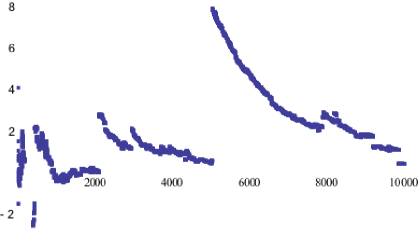
Figure 3.1. Law of large numbers for iid random variables not possesing expactations

Example 6.

As far as speed of convergence is concerned true is the following Katz’ Theorem being generalization earlier Erdös Theorem.

Theorem 15 (Katz).

Let $\left\{X_{i}\right\}_{i\geq 1}$ be a sequence of independent random variables having identical distributions such that $EX_{1}=0$. Then $E\left|X_{1}\right|^{t}<\infty$ for some $t\geq 1$ if and only if,:

$$\sum_{n\geq 1}n^{t-2}P\left(\left|\frac{\sum_{i=1}^{n}X_{i}}{n}\right|\geq\varepsilon\right)<\infty$$

for any $\varepsilon>0.$

Proof.

see [Rév67]. ∎

Having different distributions

For simplicity, we will be concerned with only classical case, i.e. when weights are equal to $1$. In this situation, we have classical Gniedenko&Kolmogorov Theorem [GK54]

Theorem 16 (Gniedenko-Kolmogorov).

Sequence $\left\{X_{i}\right\}_{i\geq 1}$ satisfies SLLN if and only if, :

$$\sum_{k\geq 1}^{n}P\left(\left|X_{k}-m(X_{k})\right|\geq n\right)\underset{n\rightarrow\infty}{\rightarrow}0,$$

$$\frac{1}{n^{2}}\sum_{k\geq 1}^{n}\int_{\left|x\right|\leq n}\left(x-m(X_{k})\right)^{2}dF_{k}(x)\underset{n\rightarrow\infty}{\rightarrow}0,$$

where $F_{k}(x)$ is cdf of a random variable $X_{k}$ and $m(X_{k})$ is its median.

Proof.

Sketch of the proof. Proof of necessity of the above-mentioned conditions is somewhat arduous and strongly uses the properties of characteristic functions hardly mentioned in this book. We will not present here this proof of necessity, since, one would have to present in detail needed properties of characteristic functions. It is presented, e.g. in [Rév67].

Proof of sufficiency of the conditions defined in this theorem is somewhat typical, it utilizes the truncation method, used already e.g. in the proof of theorems 14.

Let us denote:

$$X_{k}^{\prime} =X_{k}-m(X_{k}),$$

$$F_{k}^{\prime}(x) =P(X_{k}^{\prime}<x)=F_{k}(x+m(X_{k})),$$

$$X_{k,n}^{\prime\prime} =\left\{\begin{array}[c]{ccc}X_{k}^{\prime}&gdy&\left|X_{k}^{\prime}\right|\leq n\\ 0&gdy&\left|X_{k}^{\prime}\right|>n\end{array}\right.,$$

$$A_{n} =\frac{1}{n}\sum_{i=1}^{n}\left(m(X_{i})+EX_{i,n}^{\prime\prime}\right),$$

$$\zeta_{n}^{\prime} =\frac{1}{n}\sum_{i=1}^{n}X_{i}^{\prime},\;\zeta_{n}^{\prime\prime}=\frac{1}{n}\sum_{i=1}^{n}X_{i}^{\prime\prime},$$

$$B_{n} =\left\{\omega:\zeta_{n}^{\prime}(\omega)=\zeta_{n}^{\prime\prime}(\omega)\right\}.$$

We have of course

$$P(\overline{B}_{n})\leq\sum_{i=1}^{n}P(\left|X_{i}^{\prime}\right|>n)=\sum_{i=1}^{n}\int_{\left|x\right|>n}dF_{i}^{\prime}(x).$$

For any $\varepsilon$ we have

$$P(\left|\zeta_{n}-A_{n}\right|\geq\varepsilon)=P(B_{n})P(\left|\zeta_{n}-A_{n}\right|\geq\varepsilon|B_{n})+P(\overline{B}_{n})P(\left|\zeta_{n}-A_{n}\right|\geq\varepsilon|\overline{B}_{n}).$$

Further we have

$$P(B_{n})P(\left|\zeta_{n}-A_{n}\right| \geq\varepsilon|B_{n})\leq P\left(\left|\zeta_{n}^{\prime\prime}-E\zeta_{n}^{\prime\prime}\right|\geq\varepsilon\right)\leq\frac{\operatorname*{var}(\zeta_{n}^{\prime\prime})}{\varepsilon^{2}}$$

$$\leq\frac{1}{\varepsilon^{2}}\sum_{i=1}^{n}E\left(X_{i}^{\prime\prime}\right)^{2}.$$

Hence on the basis of assumptions, for any $\varepsilon>0$ we have:

$$P(\left|\zeta_{n}-A_{n}\right|\geq\varepsilon)\leq\frac{1}{\varepsilon^{2}n^{2}}\sum_{i=1}^{n}\int_{\left|x\right|\leq n}x^{2}dF_{k}^{\prime}(x)+\sum_{i=1}^{n}\int_{\left|x\right|>n}dF_{i}^{\prime}(x)\rightarrow 0,$$

when $n\rightarrow\infty$ . ∎

As far as speed convergence is concerned in this the case, the following Katz’ Theorem is true

Theorem 17.

Let $\left\{X_{i}\right\}_{i\geq 1}$ be a sequence of independent random variables with zero expectations, such that:

$$\exists t\in\{3,4,\ldots\}\,\exists C>0\,\forall k\in\{1,2,\ldots\}:E\left|X_{k}\right|^{t}\leq C,$$

then:

$$P\left(\left|\frac{\sum_{i=1}^{n}X_{i}}{n}\right|\geq\varepsilon\right)=O\left(\frac{1}{n^{t-1}}\right),$$

for any $\varepsilon>0.$

Proof.

Proof of this theorem is presented in [Rév67]. It is somewhat tedious and that is why we will not present it here. ∎

3.2.2. For random variables possessing variances

Proposition 11.

If

$$\operatorname*{var}\left(\frac{\sum_{n=1}^{N}\alpha_{n}X_{n}}{\sum_{n=1}^{N}\alpha_{n}}\right)\rightarrow 0;N\rightarrow\infty,$$

for some sequence $\left\{\alpha_{n}\right\}_{n\geq 1}$ satisfying conditions Theorem 14, then $\{X_{n}\}_{n\geq 1}$ satisfies WGLLN .

Proof.

By Chebyshev’s inequality we have:

$$P\left(\left|\frac{\sum_{n=1}^{N}\alpha_{n}(X_{n}-EX_{n})}{\sum_{n=1}^{N}\alpha_{n}}\right|>\varepsilon\right)\allowbreak \leq E\left(\frac{\sum_{n=1}^{N}\alpha_{n}(X_{n}-EX_{n})}{\sum_{n=1}^{N}\alpha_{n}}\right)^{2}/\varepsilon^{2}\allowbreak$$

$$=\operatorname*{var}\left(\frac{\sum_{n=1}^{N}\alpha_{n}X_{n}}{\sum_{n=1}^{N}\alpha_{n}}\right)/\varepsilon^{2}.$$

Hence, if
$\operatorname*{var}\left(\frac{\sum_{n=1}^{N}\alpha_{n}X_{n}}{\sum_{n=1}^{N}\alpha_{n}}\right)\underset{N\rightarrow\infty}{\longrightarrow}0$, then

$$\forall\varepsilon>0:\allowbreak P\left(\left|\frac{\sum_{n=1}^{N}\alpha_{n}(X_{n}-EX_{n})}{\sum_{n=1}^{N}\alpha_{n}}\right|>\varepsilon\right)\allowbreak\underset{N\rightarrow\infty}{\longrightarrow}0.$$

∎

Example 7.

In particular, if e.g. $\left\{X_{n}\right\}$ are uncorrelated and have identical variances, then the sequence $\{X_{n}\}_{n\geq 1}$ satisfies the weak law of large numbers (SLLN). Since, we have, then $\operatorname{var}\left(\sum_{i=1}^{N}X_{i}\right)\allowbreak=\allowbreak\sum_{i=1}^{N}\operatorname{var}(X_{i})$, hence $\operatorname{var}\left(\frac{\sum_{i=1}^{N}X_{i}}{N}\right)\allowbreak=\frac{\operatorname{var}(X_{1})}{N}\allowbreak\underset{N\rightarrow\infty}{\longrightarrow}0.$

Example 8.

When $\left\{X_{n}\right\}$ are uncorrelated and $\operatorname*{var}(X_{n})\approx n^{\alpha};$ $\alpha<1$, then the sequence $\{X_{n}\}_{n\geq 1}$ satisfies the weak law of large numbers (WLLN). Since arguing in the similar fashion, we have:

$$\operatorname{var}\left(\frac{\sum_{n=1}^{N}X_{n}}{N}\right)\allowbreak\approx\frac{\sum_{n=1}^{N}n^{\,\alpha}}{N^{2}}\allowbreak\approx\frac{N^{\alpha+1}}{(\alpha+1)N^{2}}\underset{N\rightarrow\infty}{\longrightarrow}0,$$

if only $\alpha<1$. This example we will illustrate by the following simulation. One took $N=4000000$ observations $\left\{\tau_{i}\right\}_{i=1}^{N}$ of the random variables of the form $\tau_{i}=i^{\beta}(\xi_{i}-E\xi_{i})$, where the random variables $\left\{\xi_{i}\right\}$ are independent and have the same distributions with cdf given by (3.2.4) for $\gamma=\frac{7}{3}$. One took $\beta=\frac{6}{14}$. Let us notice that then $\operatorname*{var}(\tau_{i})=\frac{\gamma}{(\gamma-2)(\gamma-1)^{2}}i^{2\beta}$, hence $\alpha=2\beta=\frac{6}{7}$. One obtained the following course of averages $Y_{n}=\frac{1}{n}\sum_{i=1}^{n}\tau_{i}$, $n\geq 1$. Again, as before sampling at every $K\allowbreak=\allowbreak 200$, i.e. number of iteration $=$ number on the plot times $200$.

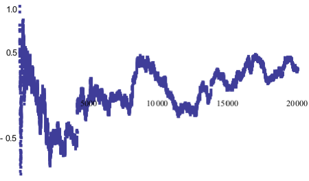
Figure 3.2. Weak law of large numbers for independent random variables having increasing variances

As one can see the convergence is rather very slow.

3.3. Strong laws of large numbers

Let us notice that Lemmas 4 and 7 supply tools to examine the conditions under which generalized, strong laws of large numbers is satisfied. As we mentioned before, the sequence of Riesz’s means $\left\{\bar{X}_{n}=\frac{\sum_{i=0}^{n-1}\alpha_{i}X_{i+1}}{\sum_{i=0}^{n-1}\alpha_{i}}\right\}_{n\geq 1}$ of the sequence $\left\{X_{i}\right\}_{i\geq 1}$ with respect to the sequence $\left\{\alpha_{i}\right\}_{i\geq 0}$ satisfies the following recursive equation:

$$\bar{X}_{n+1}=(1-\mu_{n})\bar{X}_{n}+\mu_{n}X_{n+1},$$

where $\left\{\mu_{i}\right\}_{i\geq 0}$ $=\allowbreak$ $\overline{\left\{\alpha_{i}\right\}_{i\geq 0}}.$

Remark 22.

Let us notice also, that for sequences of the random variables $\left\{X_{i}\right\}_{i\geq 1}$, having second moments and satisfying conditions:

$$\sum_{i\geq 0}\mu_{i}^{2}X_{i+1}^{2} <\infty\,\,\;a.s.~{},$$

$$\sum_{i\geq 1}\mu_{i}\bar{X}_{i}^{2} <\infty\,\,\;a.s.~{},$$

convergence of the sequence $\left\{\bar{X}_{n}\right\}_{n\geq 1}$ to zero one can prove in two ways.
Firstly, one can prove convergence a.s. of the series $\sum_{n\geq 1}\mu_{n}\bar{X}_{n}X_{n+1}$, which in the light of Lemma 7, is equivalent to proving convergence a.s. of the sequence $\left\{\bar{X}_{n}\right\}$ to zero.
Secondly, one can prove convergence a.s. of the series $\sum_{i\geq 0}\mu_{i}X_{i+1}$, which in light of Lemma 4 implies convergence a.s. sequence $\left\{\bar{X}_{n}\right\}$ to zero.

Remark 23.

If we choose the second method proposed in the previous remark, to have almost sure convergence of the series $\sum_{i\geq 0}\mu_{i}X_{i+1}$, we have also almost sure convergence series of the form $\sum_{i\geq 0}\mu_{i}^{\prime}X_{i+1}$, where the sequence is normal $\left\{\mu_{i}^{\prime}\right\}_{i\geq 0}$ is selected, that e.g. number series
$\sum_{i\geq 1}\left|\mu_{i}-\beta\mu_{i}^{\prime}\right|E\left|X_{i+1}\right|$ is convergent for some $\beta$ (compare corollary 4). Let us recall that a bit different sequences $\left\{\mu_{i}\right\}_{i\geq 0}$ and $\left\{\mu_{i}^{\prime}\right\}$ may imply very different conjugate $\left\{\alpha_{i}\right\}$ and $\left\{\alpha_{i}^{\prime}\right\}$ such that $\overline{\left\{\alpha_{i}\right\}}\allowbreak=\allowbreak\left\{\mu_{i}\right\}$ and $\overline{\left\{\alpha_{i}^{\prime}\right\}}\allowbreak=\allowbreak\left\{\mu_{i}^{\prime}\right\}$. Hence, e.g. if we have proven convergence of the series $\sum_{i\geq 1}\frac{X_{i}}{i}$, then of course sequence $\left\{\frac{\sum_{i=1}^{n}X_{i}}{n}\right\}_{n\geq 1}$ converges to zero. On the other hand, since series $\sum_{i\geq 1}\frac{X_{i}}{i}$ converges, then converges also series $\sum_{i\geq 1}\frac{2X_{i}}{i+1}$ (why? and what else has to be assumed about the moments? we leave it as an exercise to the reader), hence converges to zero also sequence $\left\{\frac{\sum_{i=1}^{n}iX_{i}}{\sum_{i=1}^{n}i}\right\}_{n\geq 1}$ (we have $\overline{\left\{i+1\right\}}=\left\{\frac{2}{i+2}\right\})$. Similarly, one can show that the sequence $\left\{\frac{\sum_{i=1}^{n}i^{2}X_{i}}{\sum_{i=1}^{n}i^{2}}\right\}_{n\geq 1}$ converges a.s. to zero. Why? and what additional technical assumptions have to be made? Formulation and justification of respective simple fact again we leave to the reader.

3.3.1. For independent random variables

Having identical distributions

We will start with the classical Kolmogorov’s result. Proof of this theorem will not be however classical in the sense, that it is different from the original Kolmogorov’s proof and uses theorems on reverse martingale convergence and $0-1$ Hewitt-Savege’ law;

Theorem 18 (Kolmogorow).

If $\{X_{n}\}_{n\geq 1}$ are independent random variables having identical distributions, in order that it satisfied SLLN it is necessary and sufficient that $E\left|X_{1}\right|<\infty.$

Proof.

Let us denote $S_{n}=\sum_{i=1}^{n}X_{i}$, $\mathcal{B}_{-n}=\sigma(S_{n},S_{n+1},\ldots)\;,n=1,2,\ldots\;$. Let us notice that $S_{n}=\allowbreak E(S_{n}|\mathcal{B}_{-n})=\allowbreak\sum_{i=1}^{n}E(X_{i}|\mathcal{B}_{-n})=\allowbreak nE(X_{1}|\mathcal{B}_{n})\,\;a.s.$, since $E(X_{1}|\mathcal{B}_{n})=E(X_{i}|\mathcal{B}_{n})$ a.s. for $i\leq n$ because of symmetry. Hence,

$$E(X_{1}|\mathcal{B}_{-n})=S_{n}/n\;a.s.~{}.$$

Moreover, we have of course

$$E(E(X_{1}|\mathcal{B}_{-n+1})|\mathcal{B}_{-n})\allowbreak=E(\frac{S_{n-1}}{n-1}|\mathcal{B}_{-n})\allowbreak=\frac{(n-1)E(X_{1}|\mathcal{B}_{-n})}{n-1}\allowbreak=E(X_{1}|\mathcal{B}_{-n}),$$

since of course $\mathcal{B}_{-n}\supseteq\mathcal{B}_{-n-1},\;n=1,2,\ldots$. Further, we have $E\left|E(X_{1}|\mathcal{B}_{-n})\right|\leq E\left|X_{1}\right|$. Hence, one can make use of Theorem 46. Now we deduce, that the sequence $\left\{S_{n}/n\right\}$ converges with probability $1$. Let $L$ denote this the limit. Events $\left\{\omega:L(\omega)<x\right\}$ are symmetric in the sense of definition 15. Now by $0-1$ Hewitt-Savege’ law (see Appendix A.11) it follows that the probability of this event is $0$ or $1$. In other words cdf of a random variable $L$ is a jump function having one jump, that is the random variable $L$ has degenerated distribution. Consequently there exists such constant $c$, that $P(L=c)=1$. Being aware that we have also convergence in $L_{1}$ (family of the random variables $\left\{S_{n}/n\right\}_{n\geq 1}$ is uniformly integrable see Appendix A.6), we have: $c=EL=\underset{n\rightarrow\infty}{\lim}E\frac{S_{n}}{n}=EX_{1}.$

Let us suppose now, that the sequence $\left\{S_{n}/n\right\}$ converges almost surely to a finite limit In such a case this sequence on the basis of Proposition 10, as well as the sequence $\left\{X_{n}/n\right\}$ converges to a finite limit (equal to zero). If $E\left|X_{1}\right|=\infty$, then as we know by Proposition 3 we would have $\underset{n\rightarrow\infty}{\lim\sup\,}\frac{\left|X_{n}\right|}{n}=\infty$. Hence, we must have $E\left|X_{1}\right|<\infty.$ ∎

In the sequel, we will consider necessary and sufficient conditions for the SGLLN to be satisfied under the assumption, that $E\left|X_{1}\right|\allowbreak<\allowbreak\infty$. It will be the result of B. Jamison, S. Orey and W. Pruitt from the paper [JOP65] .

Let $\left\{\alpha_{i}\right\}_{i\geq 0}$, $\alpha_{0}=1$ be a sequence weights, a $\left\{X_{i}\right\}_{i\geq 1}$ sequence independent random variables having identical distributions. We will consider a sequence:

$$M_{n}=\frac{\sum_{i=0}^{n-1}\alpha_{i}X_{i+1}}{\sum_{i=0}^{n-1}\alpha_{i}}$$

and examine its convergence with probability $1$ to a constant. Let us recall that the sequence $\left\{M_{n}\right\}_{n\geq 1}$ satisfies the following recurrent relationship:

(3.3.1) $$M_{n+1}=(1-\mu_{n})M_{n}+\mu_{n}X_{n+1}.$$

Let us denote $\overline{\left\{\alpha_{i}\right\}}_{i\geq 0}=\left\{\mu_{i}\right\}_{i\geq 0}$, i.e. $\mu_{i}=\alpha_{i}/\sum_{k=0}^{i}\alpha_{k}$, $i\geq 1.$

Remark 24.

If $\sum_{i\geq 0}\alpha_{i}<\infty$ or equivalently $\sum_{i\geq 0}\mu_{i}<\infty$, then the convergence of the sequence $\left\{M_{n}\right\}$ is equivalent to the convergence of the series $\sum_{i\geq 0}\alpha_{i}X_{i+1}$. This series except for the trivial case of degenerated distribution of the random variable $X_{1}$ cannot converge to a constant. Hence, if $\sum_{i\geq 0}\alpha_{i}<\infty$, then LLN is not satisfied.

Remark 25.

Thus, let us assume that $\sum_{i\geq 0}\mu_{i}=\infty$. If LLN is satisfied, i.e. the sequence of the random variables $\left\{M_{n}\right\}_{n\geq 1}$ converges to a constant, then from the identity (3.3.1) it follows that $\mu_{n}\rightarrow 0$, as $n\rightarrow\infty$ and moreover, that $\mu_{n}X_{n+1}\rightarrow 0$ with probability $1$, as $n\rightarrow\infty.$

Let $N(x)$, $x>0$ denote the number of those $n$, for which $1/x\leq\mu_{n-1}$, i.e. $N(x)=\#\left\{n:\frac{1}{\mu_{n-1}}\leq x\right\}.$

Proposition 12.

Let

(3.3.2) $$N(x)=\sum_{n\geq 1}I\left(x\geq 1/\mu_{n-1}\right),$$

then the function $N(x)$ is a nondecreasing step function, with jumps of size $1$, at values of the sequence $\left\{\frac{1}{\mu_{n-1}}\right\}_{n\geq 1}.$

Proof.

Obvious. It follows directly from the definition. ∎

We have also the following lemma.

Lemma 12.

If the sequence $\left\{M_{n}\right\}_{n\geq 1}$ defined by the relationship (3.3.1) converges to a constant, then

$$\forall c>0:EN\left(c\left|X_{1}\right|\right)<\infty.$$

Proof.

We saw already that, convergence of the sequence $\left\{M_{n}\right\}$ to a constant implies convergence of the sequence $\left\{\mu_{n}X_{n+1}\right\}_{n\geq 1}$ to zero with probability $1$. In other words, the event $\left\{\mu_{n}\left|X_{n+1}\right|>\varepsilon\right\}$ occurs a finite number of times, for every $\varepsilon>0$. From assertion $iii)$ of the Borel-Cantelli Lemma (see Appendix A.3) it follows that taking into account independence of the random variables $X_{i}$, $i>0$ we have

$$\sum_{i\geq 0}P\left(\mu_{i}\left|X_{i+1}\right|\geq\varepsilon\right)<\infty.$$

Due to the assumption of the same distributions of the random variables $\{X_{n}\}_{n\geq 1}$ the last condition can be presented the following way, due to formula(3.3.2), :

$$\sum_{i\geq 0}\int_{\left|x\right|\geq\varepsilon/\mu_{i}}dF(x)=\int\sum_{i\geq 1}I(\left|x\right|\geq\varepsilon/\mu_{i-1})dF(x)=\int N\left(\frac{\left|x\right|}{\varepsilon}\right)dF(x),$$

where $F$ denotes cdf of the random variable $X_{1}.$ ∎

Theorem 19.

Let $\left\{X_{n}\right\}_{n\geq 1}$ be a sequence of independent random variables having identical distributions, and such that $E\left|X_{1}\right|<\infty$, and let $\left\{\alpha_{i}\right\}_{i\geq 0}$ be a sequence of positive weights. Sequence$\{X_{n}\}_{n\geq 1}$ satisfies generalized MLLN with weights $\left\{\alpha_{i}\right\}_{i\geq 0}$ if and only if,

(3.3.3) $$\text{ }\underset{x\rightarrow\infty}{\lim\inf}\,\frac{N(x)}{x}<\infty,$$

where we denoted:

$$N(x)=\#\{n:\frac{\sum_{i=0}^{n-1}\alpha_{i}}{\alpha_{n-1}}\leq x\},$$

for positive $x.$

Proof.

Without loss of generality, let us assume that the random variables $\{X_{n}\}_{n\geq 1}$ have zero expectations. The main idea of the proof consists on considering ”truncated” random variables $\left\{Y_{n}\right\}_{n\geq 1}$ defined in the following way:

$$Y_{n}\allowbreak=\allowbreak X_{n}I\left(\left|X_{n}\right|<\frac{\sum_{i=0}^{n-1}\alpha_{i}}{\alpha_{n-1}}\right).$$

We have:

$$\sum_{n\geq 1}P(Y_{n}\neq X_{n})=\sum_{n\geq 1}P\left(\left|X_{n}\right|\geq\frac{\sum_{i=0}^{n-1}\alpha_{i}}{\alpha_{n-1}}\right)=$$

$$=\sum_{n\geq 1}P\left(\left|X_{1}\right|\geq\frac{\sum_{i=0}^{n-1}\alpha_{i}}{\alpha_{n-1}}\right)=E\sum_{n\geq 1}I\left(\left|X_{1}\right|\geq\frac{\sum_{i=0}^{n-1}\alpha_{i}}{\alpha_{n-1}}\right)=EN(\left|X_{1}\right|).$$

We utilized here identity of distributions of the variables $\{X_{n}\}_{n\geq 1}$, part ii) of Proposition 12 and the formula 2.1.2. Hence, if $EN(\left|X_{1}\right|)<\infty$, then from Borel-Cantelli Lemma, it will follow, that it is enough to examine random variables $\left\{Y_{n}\right\}_{n\geq 1}$. However condition (3.3.3) guarantees, that $E\left|X_{1}\right|<\infty$ $\Rightarrow$ $EN(\left|X_{1}\right|)<\infty$. Let us denote

$$T_{n}=\sum_{i=0}^{n-1}\alpha_{i}Y_{i+1}/\sum_{i=0}^{n-1}\alpha_{i}.$$

Let us also notice, that since the events $\left\{Y_{i}\neq X_{i}\right\}_{i\geq 1}$ have occured only a finite number of times, we must have $EY_{n}\rightarrow EX_{1}$, when $n\rightarrow\infty$. Thus, if we will show, that

(3.3.4) $$\sum_{i=0}^{n-1}\alpha_{i}(Y_{i+1}-EY_{i+1})/\sum_{i=0}^{n-1}\alpha_{i}\rightarrow 0\;a.s.$$

as $n\rightarrow\infty$, then the generalized strong law of large numbers will be satisfied, i.e. we will have the following convergence

$$\sum_{i=0}^{n-1}\alpha_{i}(X_{i+1}-EX_{i+1})/\sum_{i=0}^{n-1}\alpha_{i}\rightarrow 0\;a.s.$$

as $n\rightarrow\infty$. From Lemma 4 it follows that for the condition (3.3.4) to be satisfied it is enough that the series

(3.3.5) $$\sum_{i\geq 1}\mu_{i}(Y_{i+1}-EY_{i+1}),$$

converge almost surely, whereas usually we denoted $\mu_{n}=\alpha_{n}/\sum_{i=0}^{n}\alpha_{i}$. The sequence of partial sums of this series is (taking into account independence of the random variables $\left\{Y_{i}\right\}_{i\geq 1})$ a martingale. Hence, it is enough to, e.g., that the series

(3.3.6) $$\sum_{i\geq 1}\mu_{i}^{2}\operatorname*{var}(Y_{i+1})$$

and the respective martingale are being convergent almost surely and consequently strong law of large numbers is being satisfied. Let us examine the condition (3.3.6). We have:

$$\sum_{i\geq 1}\mu_{i}^{2}\int_{\mathbb{R}}x^{2}I(\left|x\right|<1/\mu_{i})dF(x)$$

$$=\int_{\mathbb{R}}x^{2}\left(\sum_{i\geq 1}\mu_{i}^{2}I(\left|x\right|<1/\mu_{i})\right)dF(x),$$

where we denoted by $F(x)$ the cdf of random the variable $X_{1}$. We have further:

$$\sum_{i\geq 1}\mu_{i}^{2}I(\left|x\right|<1/\mu_{i})=\sum_{\left\{i:\left|x\right|<1/\mu_{i}\right\}}\mu_{i}^{2}.$$

From the remark concerning jumps of the function $N(x)$, it follows that:

$$\sum_{\left\{i:\left|x\right|<1/\mu_{i}\leq z\right\}}\mu_{i}^{2}=\int_{\left|x\right|<y\leq z}\frac{dN(y)}{y^{2}}.$$

In the last integral let us integrate by parts. We get, then:

$$\int_{\left|x\right|<y\leq z}\frac{dN(y)}{y^{2}}=\frac{N(z)}{z^{2}}-\frac{N(\left|x\right|)}{x^{2}}+2\int_{\left|x\right|<y\leq z}\frac{N(y)}{y^{3}}dy.$$

Let us notice also, that

$$\frac{N(z)}{z^{2}} =-\int_{z}^{\infty}d(\frac{N(t)}{t^{2}})$$

$$=-\int_{z}^{\infty}\frac{dN(t)}{t^{2}}+2\int_{z}^{\infty}\frac{N(t)}{t^{3}}dt\leq 2\int_{z}^{\infty}\frac{N(t)}{t^{3}}dt.$$

Hence

$$\int_{\left|x\right|<y\leq z}\frac{dN(y)}{y^{2}} \leq 2\left(\int_{z}\frac{N(t)}{t^{3}}dt+\int_{\left|x\right|<y\leq z}\frac{N(y)}{y^{3}}dy\right)$$

$$=2\int_{\left|x\right|}^{\infty}\frac{N(y)}{y^{3}}dy.$$

Thus, we have:

$$\sum_{i\geq 1}\mu_{i}^{2}\int_{\mathbb{R}}x^{2}I(\left|x\right|<1/\mu_{i})dF(x)\leq 2\int x^{2}\int_{\left|x\right|}^{\infty}\frac{N(y)}{y^{3}}dydF(x)\leq$$

$$2\int_{\mathbb{R}}x^{2}\int_{\left|x\right|}^{\infty}\frac{M}{y^{2}}dydF(x)=2\int_{\mathbb{R}}x^{2}\frac{M}{\left|x\right|}dF(x)=2ME\left|X_{1}\right|,$$

where we denoted $\underset{x>0}{\sup}\frac{N(x)}{x}=M$. Hence, we have shown, that series (3.3.5) converges, consequently, that the generalized strong law of large numbers is satisfied.

Let us concentrate now on the sufficient condition. We will prove indirectly. Let us assume that $\underset{x\rightarrow\infty}{\lim\sup\,}\frac{N(x)}{x}\allowbreak=\allowbreak\infty$. It means that there exists such number sequence $\left\{x_{i}\right\}_{i\geq 1}$, that $\frac{N(x_{k})}{x_{k}}\rightarrow\infty$, as $k\rightarrow\infty$. Hence, we can select such a sequence $\left\{f_{k}\right\}_{k\geq 1}$ of positive numbers, summing to one such that $\sum_{i\geq 1}x_{i}f_{i}<\infty$ and $\sum_{i\geq 1}f_{i}N(x_{i})\allowbreak=\allowbreak\infty$. Treating sequence $\left\{f_{i}\right\}$ as step sizes of some some random variable $\left|X_{1}\right|$, we see that $E\left|X_{1}\right|<\infty$, however that $EN\left(\left|X_{1}\right|\right)=\infty$. The last condition does not allow that SLLN be satisfied in the light of Lemma 12. ∎

Remark 26.

Notice that in the classical case, i.e. when $\mu_{n}\allowbreak=\allowbreak 1/(n+1)$, $n\geq 0$ we have $N(x)\allowbreak=\allowbreak\left\lfloor x\right\rfloor$, i.e. $N(x)$ is equal to the largest integer not exceeding $x$. We have, then of course $\underset{x\rightarrow\infty}{\lim\sup}\frac{N(x)}{x}\leq 1.$

Example 9.

The above mentioned Theorem will also be illustrated by the following example.
Let $\left\{\xi_{i}\right\}_{i\geq 1}$ be a sequence of independent random variables having identical distributions. Let us assume that $\xi_{1}\sim F_{\gamma}(x)$, $\gamma>1$, where $F_{\gamma}$ is defined by (3.2.4). Then of course we have $E\xi_{1}=\frac{\gamma}{\gamma-1}$. Further, let $\mu_{i}=\frac{4(i+1)}{(i+2)^{2}};i\geq 0$, i.e. $\left\{\frac{4(i+1)}{(i+2)^{2}}\right\}=\overline{\left\{(i+1)^{2}\right\}}$ and $X_{n}=\sum_{i=1}^{n}i^{2}\xi_{i}/\sum_{i=1}^{n}i^{2}$. In this example we took $\gamma=\frac{5}{4}$, i.e. $E\xi_{1}=5$. Moreover, let us notice that $\xi_{1}$ does not have a variance.

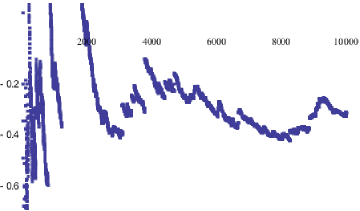
Figure 3.3. Strong law of large numbers for independent random variables not possesing variances

In order to omit technical difficulties we presented on the plot only every $K=200$’th average (i.e. $X_{200n}$; $n\allowbreak=\allowbreak 1,...$). Hence, the plot is based on $N=2000000$ observations. Let us notice also, that convergence is rather slow. It follows from the fact, that distribution of the random variable $\xi_{1}$ has the so-called ”fat tails”, i.e. function $1-F_{\gamma}(x)$ slowly decreases as $x\rightarrow\infty$. It means simply that relatively often we get very large values of $\xi_{i}$. To illustrate this, below we present a table of numbers of records of observations $\left\{\xi_{i}\right\}$ and values of these records that is the table of numbers $\left(m,M_{m}\right)$, where these numbers are defined recursively $m(0)\allowbreak=0$, $\allowbreak m(1)\allowbreak=\allowbreak 1$, $m(n+1)\allowbreak=\allowbreak\min\{j:\xi_{j}>M_{m(n)}\}$ and $\xi_{n}\allowbreak=\allowbreak M_{m(n)}$.
${\small 3}$ ${\small 14}$ $15$ $17$ $42$ $189$ $327$ $99184$ $101942$ $461831$ $-2.20$ $-0.27$ $0.68$ $1.21$ $39.55$ $102.11$ $4602.51$ $9292.62$ $73342.5$ $84457$
As one can see the first record happened to observation $3$ and had valued $-2.2$, the second in the $14$-th observation and had value $-.27$ and so on. Finally, the $11$-th record happened to observation $13338828$ and had value equal $87444$ .

Having different distributions

Recall that in the case of identical distributions of the sequence of independent random variables, it was sufficient to assume the existence of expectations to get  MLLN (compare theorem 18) to be satisfied by $\{X_{n}\}_{n\geq 1}$. The case of different distributions is different. It turns out that even the existence of second moments is not enough. It turns out that these moments must satisfy some additional conditions. This case will be treated in a whole in the next section together with the case of dependent elements of the sequence $\{X_{n}\}_{n\geq 1}$. Whereas here we will present examples of sequences of independent random variables, not satisfying MLLN. Interesting and instructive examples presented below, are modifications of examples taken from the book of Révész [Rév67].

Example 10.

Let sequence $\left\{\sigma_{n}^{2}\right\}_{n\geq 1}$ will be such sequence of positive numbers, that

(3.3.7) $$\sum_{n\geq 1}\frac{\sigma_{n}^{2}}{n^{2}}=\infty.$$

Let sequence $\{X_{n}\}_{n\geq 1}$ be a sequence independent random variables having the following distributions:

$$P(X_{n} =n)=P(X_{n}=-n)=\frac{\sigma_{n}^{2}}{2n^{2}},$$

$$P(X_{n} =0)=1-\frac{\sigma_{n}^{2}}{n^{2}},$$

when $\sigma_{n}^{2}\leq n^{2}$ and

$$P(X_{n}=\sigma_{n})=P\left(X_{n}=-\sigma_{n}\right)=\frac{1}{2},$$

when $\sigma_{n}^{2}>n^{2}$. Let us notice that $EX_{n}=0$, $\operatorname*{var}(X_{n})=\sigma_{n}^{2,}$ and Moreover, $P(\left|X_{n}\right|\geq n)\allowbreak\geq\allowbreak\sigma_{n}^{2}/n^{2}$. From the last estimation, it follows that $P(\underset{n\rightarrow\infty}{\lim}\left|\frac{X_{n}}{n}\right|=0)\allowbreak=\allowbreak 0$, in other words necessary condition for the SLLN to be satisfied is not satisfied (see Proposition 10). Thus, we have constructed a sequence of independent random variables with given variances, that is not satisfying SLLN. Condition (3.3.7) indicates how quickly variances of elements of the sequence of independent random variables have to increase, so that MLLN is not satisfied for this sequence.

In connection with the previous example, there appears a question, can one select the sequence of weights in such a way, as to make a sequence of independent random variables having increasing variances satisfy a generalized SLLN. It turns out that one can give a similar condition to (3.3.7), imposed on the speed with which variances of elements of the sequence $\{X_{n}\}_{n\geq 1}$ increase, so that for any system of weights generalized SLLN is not satisfied.

To describe this situation more precisely, let us consider the sequence $\{X_{n}\}_{n\geq 1}$ of independent random variables such that $EX_{n}=0$, $\operatorname*{var}(X_{n})=\sigma_{n}^{2}$. We have the following simple lemma.

Lemma 13.

$\min\operatorname*{var}(\sum_{i=1}^{n}a_{i}X_{i})=1/\sum_{i=1}^{n}1/\sigma_{i}^{2}$, where the minimum is taken over all systems of positive numbers $\left\{a_{i}\right\}_{i=1}^{n}$, such that $\sum_{i=1}^{n}a_{i}=1.$

Proof.

We have

$$1=\allowbreak\sum_{i=1}^{n}a_{i}\allowbreak=\sum_{i=1}^{n}a_{i}\sigma_{i}\frac{1}{\sigma_{i}}\leq\sqrt{\sum_{i=1}^{n}a_{i}^{2}\sigma_{i}^{2}}\sqrt{\sum_{i=1}^{n}1/\sigma_{i}^{2}}.$$

Remembering, that $\operatorname*{var}(\sum_{i=1}^{n}a_{i}X_{i})=\sum_{i=1}^{n}a_{i}^{2}\sigma_{i}^{2},$ we see that $\operatorname*{var}(\sum_{i=1}^{n}a_{i}X_{i})\geq 1/\sum_{i=1}^{n}1/\sigma_{i}^{2}$. It is known, that equality in inequality Schwarz that we applied satisfies, when $a_{i}\sigma_{i}=\lambda/\sigma_{i};i=1,\ldots,n$ for some $\lambda$. Hence, taking into account condition $1=\allowbreak\sum_{i=1}^{n}a_{i}\allowbreak$, when $a_{i}=\eta/\sigma_{i}^{2}$, where $\eta=1/\sum_{i=1}^{n}1/\sigma_{i}^{2}$. We have moreover ,

$$\operatorname*{var}(\sum_{i=1}^{n}X_{i}\eta/\sigma_{i}^{2})\allowbreak=\allowbreak\eta^{2}\sum_{i=1}^{n}\sigma_{i}^{2}/\sigma_{i}^{4}\allowbreak=\allowbreak 1/\sum_{i=1}^{n}1/\sigma_{i}^{2}.$$

∎

Having this lemma let us assume, that our sequence of the random variables $\{X_{n}\}_{n\geq 1}$ is such that

(3.3.8) $$\sum_{i\geq 1}\frac{1}{\sigma_{i}^{2}}<\infty.$$

Then of course we would have for any system of weights $\left\{a_{in}\right\}_{i\geq 1}$ such that $\forall n=1,2,\ldots\;\sum_{i=1}^{n}a_{in}=1,$

$$\operatorname*{var}(\sum_{i=1}^{n}a_{in}X_{i})\geq 1/\sum_{i=1}^{n}1/\sigma_{i}^{2}\geq 1/\sum_{i\geq 1}\frac{1}{\sigma_{i}^{2}}>0.$$

If the sequence $\{X_{n}\}_{n\geq 1}$ satisfied generalized $SLLN$, then of course respective sequence of averages (i.e. the sequence $\sum_{i=1}^{n}a_{in}X_{i})$ would converge with probability to zero. In particular, the sequence of variances of its elements would converge to zero, which is impossible in this case. Thus, the sequence of independent random variables having variances satisfying condition (3.3.8) does not satisfy any generalized SLLN.

3.3.2. For random variables possessing variances

For uncorrelated random variables.

Properties of the sequence of averages $\left\{\bar{X}_{i}\right\}_{i\geq 1}$ are described in Lemmas 7 and 9. For convenience, we will recall below, these results compiled in one, new lemma.

Lemma 14.

If the series $\sum_{i\geq 1}\mu_{i}^{2}EX_{i+1}^{2}$ is convergent, then:
i) series $\sum_{i\geq 0}\mu_{i}\bar{X}_{i}^{2}$ is convergent almost surely,
ii) sequence $\left\{\frac{\sum_{i=1}^{n}\alpha_{i}\bar{X}_{i}^{2}}{\sum_{i=1}^{n}\alpha_{i}}\right\}_{n\geq 1}$ converges almost surely to zero,
iii)  $\bar{X}_{n}$ $\underset{n\rightarrow\infty}{\longrightarrow}$ $0$ if and only if, series $\sum_{i\geq 0}\mu_{i}\bar{X}_{i}X_{i+1}$ is convergent almost surely,
iv) Let $\left\{n_{k}\right\}_{k\geq 1}$ be a sequence of indices defined by the relationship $\sum_{i=n_{k}+1}^{n_{k+1}}\mu_{i}\allowbreak=\allowbreak O(1)$, then $\bar{X}_{n_{k}}\underset{k\rightarrow\infty}{\longrightarrow}0$ almost surely.

Proof.

Proofs of i), ii), iii), iv) are repetitions of proofs of assertions 1, 3, 7, 4 of Lemma 9. ∎

Remark 27.

Let us notice that having assumed convergence of the series of assertion i) Lemma 14 one can prove (making use of the iterative form, the properties of the sequence $\left\{\mu_{i}\right\}_{i\geq 0}$ and of Lemma 4) not only convergence of the sequence of assertion ii) of this lemma, but also the convergence of e.g. sequence

$$\left\{\frac{\sum_{i=1}^{n}\alpha_{i}\left(\sum_{j=0}^{i}\alpha_{j}\right)^{k-1}\bar{X}_{i}^{2}}{\left(\sum_{j=0}^{n}\alpha_{j}\right)^{k}}\right\}_{n\geq 1}$$

for $k=1,2,\ldots\,.$

Moreover, we have of course Menchoff ’ Theorem 10 to examine of the general case of the sequence $\left\{X_{n}\right\}_{n\geq 1}$ and Theorem 43 (Doob) for examining of the case of the sequence $\left\{X_{n}\right\}_{n\geq 1}$ consisting of martingale differences, which are used to examine almost sure convergence of the sequence $\left\{\bar{X}_{n}\right\}_{n\geq 1},$together with Lemma 4 gives the following theorem.

Theorem 20.

Let the sequence $\left\{X_{n}\right\}_{n\geq 1}$ consist of uncorrelated random variables having finite second moments.
If series $\sum_{i\geq 1}\mu_{i}^{2}EX_{i+1}^{2}\left(\ln i\right)^{2}$ is convergent
or if convergent is the series $\sum_{i\geq 1}\mu_{i}^{2}EX_{i+1}^{2}$ and additionally sequence $\left\{X_{n}\right\}_{n\geq 1}$ consist of martingale differences, then:

1. $\bar{X}_{n}$ $\underset{n\rightarrow\infty}{\longrightarrow}$ $0$ almost surely

2. series $\sum_{i\geq 1}\mu_{i}X_{i+1}$ converges almost surely to some square integrable random variable $S.$

If additionally system $\{X_{n}\}_{n\geq 1}$ is PSO (see page. 12), then we have Lemma 11, and if additionally we know, that $\sup_{n\geq 1}\mu_{n}\ln n<\infty$, then we get Theorem 13.

As a corollary, we have a classical theorem concerning the sequence of independent random variables that satisfy SLLN.

Corollary 6.

Let $\left\{X_{i}\right\}_{i\geq 1}$ be a sequence independent random variables having finite variances such that $\sum_{i\geq 1}\operatorname*{var}(X_{i})/(i+1)^{2}<\infty$. Then sequence $\left\{X_{i}\right\}_{i\geq 1}$ satisfies SLLN.

Proof.

It follows from previous theorems, since, firstly the sequence $\{X_{i}\}_{i\geq 1}$ is a sequence of martingale differences, secondly we took $\mu_{i}=1/(i+1)$. ∎

Example 11.

The simplest application of Theorem 20, is to consider a sequence $\left\{X_{n}\right\}_{n\geq 1}$ with zero expectations and increasing variances e.g. following the scheme : $\operatorname{var}(X_{n})\approx\frac{n^{\alpha}}{\ln^{\beta}n}$. Then, as it follows from the above mentioned theorems, the sequence
$\left\{Y_{n}=\frac{\sum_{i=1}^{n}X_{i}}{n}\right\}_{n\geq 1}$ converges almost surely to zero, if only: either $\alpha<1$, or if $\alpha=1$ and $\beta>3$ in the general (uncorrelated) case and either $\alpha<1$, or $\alpha=1$ and $\beta>1$ of the case of martingale differences. Good illustration of SLLN in this case is the example and simulation discussed in example 8. In order to find out, how the value of the coefficient $\alpha$ influences the quality of convergence we will present new simulation. We took the same random variables, as in example 8 with the small difference that now $\beta=\frac{3}{14}$, that is $\alpha=\frac{6}{14}<0.5$. Again, as before, we expose every 1 hundredth observation, i.e. for $J=200$, $400$, $\ldots,4000000$ we present $y_{J}$

Much more interesting is, however the usage of the above mentioned theorem to examine the of speed convergence in ”ordinary” LLN. More precisely, let us assume, that we are interested in speed of convergence of the sequence $\left\{\frac{\sum_{i=1}^{n}X_{i}}{n}\right\}_{n\geq 1}$ to zero. This means that we want to find such, an increasing number sequence $\left\{\chi_{n}\right\}_{n\geq 1}$, that the sequence
$\left\{\chi_{n}\frac{\sum_{i=1}^{n}X_{i}}{n}\right\}_{n\geq 1}$ converges almost surely to zero. Such considerations will be performed in the next example.

Example 12.

Let us consider, sequence of uncorrelated random variables $\left\{X_{i}\right\}_{i\geq 1}$ such that $EX_{i}=0$, $EX_{i}^{2}=1;\allowbreak i\geq 1$. Let us set

$$Y_{n}=\frac{\sum_{i=1}^{n}X_{i}}{\sqrt{n\ln(n+1)\ln\ln^{2}(n+2)}};n\geq 1.$$

Hence $\chi_{n}=\sqrt{\frac{n}{\ln(n+1)\ln\ln^{2}(n+2)}}$. Let us present $Y_{n}$ in the iterative form.

$$Y_{n+1}=(1-\nu_{n})Y_{n}+\frac{X_{n+1}}{\sqrt{\left(n+1\right)\ln(n+2)\ln\ln^{2}\left(n+3\right)}}$$

where

$$\nu_{n}=1-\sqrt{\frac{n\ln(n+1)\ln\ln^{2}(n+2)}{\left(n+1\right)\ln\left(n+2\right)\ln\ln^{2}(n+3)}}\approx\frac{1}{2n}+\frac{1}{2n\ln n}+o(\frac{1}{n\ln n}).$$

Since, the series $\sum_{n\geq 1}\frac{1}{n\ln(n+1)\ln\ln^{2}(n+2)}$ converges, we deduce that if only additionally we will assume, that the sequence $\left\{X_{n}\right\}_{n\geq 1}$ is the sequence of martingale differences, then sequence $\left\{Y_{n}\right\}_{n\geq 1}$ converges almost surely to zero.

On the other hand, however, if one does not assume, that the sequence $\left\{X_{n}\right\}_{n\geq 1}$ consists of martingale differences, then knowing, that the series

$$\sum_{n\geq 1}\frac{1}{n\ln(n+1)\ln\ln^{2}(n+2)}\ln^{2}n,$$

does not converge then on the basis of Menchoff’ Theorem 10 we deduce that series

$$\sum_{n\geq 1}X_{n}/\sqrt{n\ln(n+1)\ln\ln^{2}(n+2)}$$

may not converge almost surely, although it does converge in mean square. It depends on further properties of distributions of variables $\left\{X_{i}\right\}_{i\geq 1}$, not only on the properties of their second moments. Similarly the sequence $\left\{Y_{n}\right\}$ may converge almost surely, or may not depending on the properties of the sequence $\left\{X_{i}\right\}_{i\geq 0}$. Following assertion iv) of  Lemma 9 there exists a subsequence of the sequence $\left\{Y_{n}\right\}_{n\geq 1}$ that converges almost surely. From the form of the sequence $\left\{\nu_{n}\right\}$ we deduce that the sequence $\left\{n_{k}\right\}$ can be chosen to be $\left\{2^{k}\right\}$. Hence, on the basis of assertion iv) of the above mentioned lemma, we deduce that $Y_{2^{k}}\underset{k\rightarrow\infty}{\longrightarrow}0$ almost surely. Moreover, from assertion ii) we infer, for example, that the sequence $\left\{\frac{\sum_{i=1}^{n}Y_{i}^{2}/\sqrt{i}}{\sqrt{n}}\right\}$ converges almost surely to zero. Strict justification of this fact, we leave to the reader as an exercise.

Let us now suppose, that weights $\left\{\alpha_{i}\right\}_{i\geq 0}$ are constant. Hence, $\mu_{i}=\frac{1}{i+1}$, $i\geq 0$, $\bar{X}_{n}=\frac{1}{n}\sum_{i=1}^{n}X_{i}$. Following remark 27 under the assumption, that series $\sum\mu_{i}\bar{X}_{i}^{2}$ is convergent with probability $1$, it follows that $\frac{\sum_{i=1}^{n}i^{2}\bar{X}_{i}^{2}}{n^{3}}\rightarrow 0$ with probability $1$ ($k=1$, $\alpha_{i}=i^{2})$. Let $\beta$ will be any nonnegative number. From assertion iii) of Lemma 6 we have:

$$A_{n}^{\beta+1}=O(n^{\beta+1}),\sum_{i=1}^{n}\left(A_{n-i}^{\beta-1}\right)^{2}\allowbreak=\allowbreak\sum_{i=1}^{n}\left(A_{i}^{\beta-1}\right)^{2}\allowbreak=\allowbreak\sum_{i=1}^{n}O(i^{2\beta-2})\allowbreak=\allowbreak O(n^{2\beta-1}).$$

Hence, $\frac{\sqrt{\sum_{i=1}^{n}\left(A_{n-i}^{\beta-1}\right)^{2}}n^{3/2}}{A_{n}^{\beta+1}}\allowbreak\cong\allowbreak O(1)$ and consequently with probability $1$ we have:

$$\left|\frac{\sum_{i=1}^{n}A_{n-i}^{\beta-1}i\bar{X}_{i}}{A_{n}^{\beta+1}}\right|\leq\frac{\sqrt{\sum_{i=1}^{n}\left(A_{n-i}^{\beta-1}\right)^{2}}n^{3/2}}{A_{n}^{\beta+1}}\sqrt{\frac{\sum_{i=1}^{n}i^{2}\bar{X}_{i}^{2}}{n^{3}}}\rightarrow 0;\,n\rightarrow\infty.$$

Hence comparing above mentioned expression with assertion iv) of Lemma 6 we see (taking $\alpha=1$ and $\beta>1)$, that the sequence $\{X_{n}\}_{n\geq 1}$ is $(C,\beta)$ summable for $\beta>1$. We have thus proved the following Theorem, being a generalization of Theorems $1$ and $2$ of the paper [Mór83a].

Theorem 21.

If $\{X_{n}\}_{n\geq 1}$ is a sequence of the random variables such that

$$\sum_{n\geq 1}\frac{EX_{n}^{2}}{(n+1)^{2}}<\infty,\;\sum_{n\geq 1}\frac{E\bar{X}_{n}^{2}}{n+1}<\infty,$$

where $\bar{X}_{n}=\frac{1}{n}\sum_{i=1}^{n}X_{i}$, then the sequence $\{X_{n}\}_{n\geq 1}$ is $(C,\alpha)$ summable for $\alpha>1$.

Remark 28.

Of course, if we will assume, that the sequence $\{X_{n}\}_{n\geq 1}$ consists of orthogonal random variables, then the first of the conditions of the above mentioned theorem entails the second one (compare assertion Lemma 14). Hence, in this case we get precisely above mentioned theorems of the quoted paper.

To end this part let us recall, that for the uncorrelated random variables condition $\sum_{n\geq 1}\frac{EX_{n}^{2}}{(n+1)^{2}}<\infty$ is not sufficient for SLLN to occur. It is so since we have the following theorem.

Theorem 22.

Let $\left\{\sigma_{n}^{2}\right\}_{n\geq 1}$ be a sequence of positive numbers such that series :

$$\,\sum_{n\geq 1}\frac{EX_{n}^{2}\ln^{2}(n+1)}{n^{2}}$$

is divergent, and a number sequence $\left\{\frac{\sigma_{n}^{2}}{n^{2}}\right\}_{n\geq 1}$ is non-increasing. Then one can construct the probability space and define a sequence $\{X_{n}\}_{n\geq 1}$ of uncorrelated random variables with zero expectations such that $EX_{n}^{2}=\sigma_{n}^{2},\;n\geq 1$ and with probability $1$

$$\underset{n\rightarrow\infty}{\lim\inf}\,\left|\frac{\sum_{i=1}^{n}X_{i}}{n}\right|=\infty.$$

Proof.

Is long and complicated, one can find it in the paper [Tan72]. ∎

For correlated random variables.

Lemmas 7 and 9 supply tools for better analysis of this of the case. We have the following theorem:

Theorem 23.

If the following series

(3.3.9) $$\sum_{n=1}^{\infty}\mu_{n}^{2}\operatorname*{var}(X_{n+1}),\;\;\sum_{n=1}^{\infty}\mu_{n}\sqrt{\operatorname*{var}(X_{n+1})\operatorname*{var}(\overline{X}_{n})},$$

are convergent, where we denoted as usually $\overline{X}_{n}\allowbreak=\allowbreak\sum_{i=0}^{n-1}\alpha_{i}X_{i+1}/\sum_{i=0}^{n-1}\alpha_{i},\;\allowbreak\overline{\left\{\alpha_{i}\right\}}\allowbreak=\allowbreak\left\{\mu_{i}\right\}$, then $\{X_{n}\}_{n\geq 1}$ satisfies generalized SLLN with weights $\left\{\alpha_{i}\right\}.$

Proof.

Let $\left\{X_{i}\right\}_{i\geq 1}$ be a sequence of the random variables possessing variances. Without loss of generality one can assume, that $EX_{i}=0$. It is easy to notice, that the sequence $\left\{\overline{X}_{n}\right\}$ satisfies the following recurrent relationship:

$$\overline{X}_{i+1}=(1-\mu_{i})\overline{X}_{i}+\mu_{i}X_{i+1}.$$

We multiply side by side this identity by itself, obtaining:

$$\overline{X}_{i+1}^{2}=(1-\mu_{i}(2-\mu_{i}))\overline{X}_{i}^{2}+\allowbreak 2(1-\mu_{i})\mu_{i}\overline{X}_{i}X_{i+1}+\allowbreak\mu_{i}^{2}X_{i+1}^{2}.$$

Now we use numerical lemma 4 of chapter 2 and see that $\overline{X}_{i}^{2}$ converges to zero almost surely, when the series $\sum_{i\geq 0}\mu_{i}^{2}X_{i+1}^{2}$ and $\sum_{i\geq 0}\mu_{i}\overline{X}_{i}X_{i+1}$ converge almost surely. Now it is enough to apply Schwarz’ inequality to the series $\sum_{i\geq 0}\mu_{i}\overline{X}_{i}X_{i+1}$ and use corollary 1 of Lebesgue’ Theorem. ∎

If we set $\alpha_{i}=\frac{1}{i+1};$ $i=0,1,\ldots$, then from this Theorem follows evident corollary.

Corollary 7.

If the following series

$$\sum_{i\geq 1}\operatorname{var}(X_{i})/i^{2},\;\;\sum_{i\geq 1}\frac{1}{i}\sqrt{\operatorname{var}(X_{i+1})\operatorname{var}\left(\frac{1}{i}\sum_{k=1}^{i}X_{k}\right)}$$

are convergent, then the sequence $\left\{X_{i}\right\}_{i\geq 1}$ satisfies SLLN.

Example 13.

 Let $\left\{X_{i}\right\}_{i\geq 1}$ will consist of the following random variables:
i)

$$EX_{i}=0;i\geq 1,\left|\operatorname*{cov}(X_{i},X_{j})\right|\leq\left\{\begin{tabular}[c]{lll}$C(\max(i,j))^{\alpha}$&for&$\left|i-j\right|\leq 4$\\ $0$&for&$\left|i-j\right|>4$\end{tabular}\ ,\right.\alpha<1,$$

ii)

$$EX_{i}=0\,;i\geq 1\left|\operatorname*{cov}(X_{i},X_{j})\right|\leq\frac{C}{2^{\left|i-j\right|}};i,j\geq 1.$$

It turns out that the sequences of i) and ii) satisfy SLLN. To show this, let us notice that estimation $E\left|\bar{X}_{n}\right|^{2}$, examining convergence of series $\sum_{i\geq 1}\frac{E\left|X_{i}\right|^{2}}{i+1}$ is essential. In the case i) we have:

$$E\left|\bar{X}_{n}\right|^{2} =\frac{1}{n^{2}}E(\sum_{i=1}^{n}X_{i})^{2}\leq$$

$$\leq\frac{C}{n^{2}}(\sum_{i=1}^{n}i^{\alpha}+2\sum_{i=2}^{n}i^{\alpha}\allowbreak+2\sum_{i=3}^{n}i^{\alpha}\allowbreak+2\sum_{i=4}^{n}i^{\alpha}+\allowbreak 2\sum_{i=5}^{n}i^{\alpha}))$$

$$\leq\frac{9C}{n^{1-\alpha}}.$$

Hence for this case we have

$$\sum_{n=1}^{\infty}\operatorname*{var}(X_{n+1})/n^{2}\allowbreak\approx\sum_{n=1}^{\infty}Cn^{-(2-\alpha)},$$

while for the second

$$\sum_{n=1}^{\infty}\frac{1}{n}\sqrt{\operatorname*{var}(X_{n+1})\operatorname*{var}(\frac{1}{n}\sum_{i=1}^{n}X_{i})}\allowbreak\approx\sum_{n=1}^{\infty}\frac{C}{n^{1-\alpha/2+1/2-\alpha/2}}.$$

The first of these series converges, when $2-\alpha>1$, or $\alpha<1$, while the second series,when $3/2-\alpha>1$, i.e. when $\alpha<1/2.$

In of the case ii) we have:

$$E\left|\bar{X}_{n}\right|^{2} =\frac{1}{n^{2}}E(\sum_{i=1}^{n}X_{i})^{2}$$

$$\leq\allowbreak\frac{1}{n^{2}}(nC+\allowbreak 2C\frac{1}{2}(n-1)+\allowbreak 2C\frac{1}{4}(n-2)+\allowbreak\ldots\allowbreak+2C\frac{1}{2^{n-1}}(n-(n-1)))\allowbreak$$

$$\leq\frac{3C}{n}.$$

Hence $\sqrt{E\left|\bar{X}_{n}\right|^{2}}\approx O(1/\sqrt{n})$. Thus, the series $\sum_{i\geq 1}\frac{1}{n+1}\sqrt{E\left|\bar{X}_{n}\right|^{2}}\sqrt{E\left|X_{n+1}^{2}\right|}$ converges.

Remark 29.

Analyzing the above mentioned example, it is easy to notice, that the strong law of large numbers is satisfied also by the following sequences $\left\{X_{i}\right\}_{i\geq 1}$ of dependent random variables:

$$EX_{i}=0\,;i\geq 1,~{}\left|\operatorname*{cov}(X_{i},X_{j})\right|\leq\allowbreak\frac{C}{\eta(\left|i-j\right|)};i,j\geq 1,$$

where the function $\eta$ satisfies the condition: series $\sum_{n\geq 1}\frac{1}{n^{3/2}}\sqrt{\sum_{i=1}^{n}\frac{1}{\eta(i)}}$ is convergent. It entails, that $E\bar{X}_{n}^{2}\leq\frac{C}{n}\sum_{i=1}^{n}\frac{1}{\eta(i)}$. It is also not difficult to notice, that functions $\eta$ satisfying these conditions are e.g. $\eta(x)=\left|x\right|^{\beta};\beta>0,\,\eta(x)=\log^{1+\gamma}(1+|x|);\gamma>0$, and so on. Below we will generalize this example. Random variables satisfying the above mentioned conditions will be called quasi-stationary.

Theorem 23 gives possibility of getting the laws of large numbers for dependent random variables. Conditions for ”dependence” can be expressed in terms of the covariances of the random variables $\{X_{n}\}_{n\geq 1}$. Theorem 23 provides quick, ”easy to apply” convergence criteria. In order to present more subtle ones for SLLN to be satisfied by dependent random variables in concise form, one has to assume more about the mutual dependence of the elements of the sequence $\{X_{n}\}_{n\geq 1}$. Hence, let us consider an important class of the random variables, namely the so-called quasi-stationary random variables.

Definition 8.

Random variables $\{X_{n}\}_{n\geq 1}$ are quasi-stationary, if i) $\forall n\geq 1$: $E\left|X_{n}\right|^{2}<\infty$, ii) $\forall i,j\geq 1:$

$$\left|\operatorname{cov}(X_{i},X_{j})\right|\allowbreak\leq\allowbreak\rho(\left|i-j\right|)\allowbreak\sqrt{\operatorname*{var}(X_{i})\operatorname*{var}(X_{j})},$$

for some sequence $\left\{\rho(i)\right\}_{i\geq 0}$ nonnegative numbers such, that $\rho(0)=1$.

For such sequences we will give a generalization of Lemma 8, and also Rademacher-Menshoff’s Theorem 10. Let us suppose, that $\{X_{n}\}_{n\geq 1}$ is the sequence of quasi-stationary random variables  with zero expectations, such that $\operatorname*{var}(X_{i})=\sigma_{i}^{2}$, $\left|\operatorname{cov}(X_{i},X_{j})\right|\leq\rho(\left|i-j\right|)\sigma_{i}\sigma_{j}$. Let us introduce also the following denotations:

$$\mathbf{R}_{n}=[r_{ij}]_{1\leq i,j\leq n}=\left[\rho(|i-j|)\right]_{1\leq i,j\leq n},\;\mathbf{\xi}_{n}^{T}=[\beta_{1}\sigma_{1},\ldots,\beta_{n}\sigma_{n}].$$

We have the following generalization of Lemma 8.

Lemma 15.

Let us denote $S_{i}=\sum_{j=1}^{i}\beta_{j}X_{j}$ :$i=1,2,\ldots,n$. We have

$$E\underset{1\leq i\leq n}{\max}S_{i}^{2}=M(n)\leq O\left(\log^{2}n\right)\left(\sum_{i=0}^{n}\rho(i)\right)\sum_{i=1}^{n}\beta_{i}^{2}\sigma_{i}^{2}.$$

Proof.

Let $\nu(\omega)$ will be the smallest index such that

$$\underset{1\leq i\leq n}{\max}S_{i}^{2}=S_{\nu}^{2}.$$

Repeating part of arguments and calculations from the proof of Lemma 8 we get:

$$S_{\nu}^{2}\leq\left(\sum_{j=1}^{\nu}A_{\nu-j}^{-1/2}A_{j}^{-1/2}\left|S_{j}^{-1/2}\right|\right)^{2}\leq\sum_{j=1}^{\nu}\left(A_{\nu-j}^{-1/2}\right)^{2}\sum_{j=1}^{n}\left(A_{j}^{-1/2}\left|S_{j}^{-1/2}\right|\right)^{2}.$$

(3.3.10) $$\sum_{j=1}^{\nu}\left(A_{\nu-j}^{-1/2}\right)^{2}=1+\sum_{j=1}^{\nu}O(\frac{1}{\nu-j})=O(\ln\nu)\leq O(\ln n).$$

$$ES_{k}^{2} =\left(\sum_{i=1}^{n}\beta_{i}^{2}\sigma_{i}^{2}+2\sum_{1\leq i<j\leq n}\beta_{i}\beta_{j}\operatorname{cov}(X_{i},X_{j})\right)\leq$$

$$\leq\mathbf{\xi}_{n}^{T}\mathbf{R}_{n}\mathbf{\xi}_{n}\allowbreak\leq\allowbreak\lambda_{n}\mathbf{\xi}_{n}^{T}\mathbf{\xi}_{n},$$

where $\lambda_{n}$ denotes the greatest eigenvalue of matrix $\mathbf{R}_{n}$ (its spectral norm). Since, that spectral norm does not exceed any other matrix norm (compare theorem. 6.1.3 in [Lan69]) we have:

$$ES_{k}^{2}\leq 2\left(\sum_{i=0}^{n-1}\rho(i)\right)\sum_{i=1}^{n}\beta_{i}^{2}\sigma_{i}^{2},$$

since we have

$$\left\|R_{n}\right\|=\underset{1\leq i\leq n}{\max}\sum_{j=1}^{n}r_{ij}=\underset{1\leq i\leq n}{\max}\left(2\sum_{j=0}^{i-1}\rho(j)+\sum_{j=i}^{n-1}\rho(j)\right)\leq 2\sum_{j=0}^{n-1}\rho(j).$$

Moreover, :

$$E\sum_{j=1}^{n}\left(A_{j}^{-1/2}\left|S_{j}^{-1/2}\right|\right)^{2} =\sum_{j=1}^{n}E\left(A_{j}^{-1/2}S_{j}^{-1/2}\right)^{2}=$$

$$=\sum_{j=1}^{n}E\left(\sum_{k=1}^{j}A_{j-k}^{-1/2}\beta_{k}X_{k}\right)^{2}\leq$$

$$\leq 2\sum_{j=1}^{n}\sum_{i=0}^{j-1}\rho(i)\sum_{k=1}^{j}\beta_{k}^{2}\sigma_{k}^{2}\left(A_{j-k}^{-1/2}\right)^{2}\leq$$

$$\leq 2\sum_{k=0}^{n}\rho(k)\sum_{k=1}^{n}\beta_{k}^{2}\sigma_{k}^{2}\left(O\left(1\right)+O\left(\frac{1}{2}\right)+\ldots+O\left(\frac{1}{k}\right)\right)\leq$$

$$\leq O(\log n)\sum_{k=0}^{n}\rho(k)\sum_{k=1}^{n}\beta_{k}^{2}\sigma_{k}^{2}.$$

Combining (3.3.10) and the above mentioned result we get assertion of our lemma. ∎

Having this lemma it is easy to get Theorem similar to Rademacher-Menchoff’s Theorem.

Theorem 24.

Let $\{X_{n}\}_{n\geq 1}$ be a sequence of quasi-orthogonal random variables such that $\operatorname*{var}(X_{i})=\sigma_{i}^{2}$, $\left|\operatorname{cov}(X_{i},X_{j})\right|\leq\rho(\left|i-j\right|)\sigma_{i}\sigma_{j}$. If series

$$\sum_{i\geq 1}\beta_{i}^{2}\sigma_{i}^{2}\log^{2}i\sum_{j=0}^{i}\rho(j)$$

is convergent, then series $\sum_{i\geq 1}\beta_{i}X_{i}$ is convergent with probability $1.$

Using this theorem and making use of Lemma 4 one can easily get the following result.

Corollary 8.

Let $\{X_{n}\}_{n\geq 1}$ be a sequence of quasi-orthogonal random variables such that $\operatorname*{var}(X_{i})=\sigma_{i}^{2}$, $\left|\operatorname{cov}(X_{i},X_{j})\right|\leq\rho(\left|i-j\right|)\sigma_{i}\sigma_{j}$. If series

$$\sum_{i\geq 1}\frac{\alpha_{i-1}^{2}}{\left(\sum_{j=0}^{i-1}\alpha_{j}\right)^{2}}\sigma_{i}^{2}\log^{2}i\sum_{j=0}^{i}\rho(j)$$

is convergent, then the sequence $\left\{\frac{\sum_{i=1}^{n}\alpha_{i-1}X_{i}}{\sum_{i=1}^{n}\alpha_{i-1}}\right\}_{n\geq 1}$ is convergent with probability 1 to zero.

Also from Theorem 24 it is easy also to get the following facts.

Proposition 13.

Let $\{X_{n}\}_{n\geq 1}$ be a sequence of quasi-orthogonal random variables such that $\operatorname*{var}(X_{i})=\sigma_{i}^{2}$, $\left|\operatorname{cov}(X_{i},X_{j})\right|\leq\rho(\left|i-j\right|)\sigma_{i}\sigma_{j}$. Let $\left\{\beta_{i}\right\}_{i\geq 1}$ be a number sequence such that convergent is series:

$$\sum_{i\geq 1}\beta_{i}^{2}\sigma_{i}^{2}.$$

Then with probability $1$ we have $\sum_{i=1}^{n}\beta_{i}X_{i}=O(\log n\sqrt{\sum_{i=1}^{n}\rho(i)}).$

Further from this Proposition follows the following one:

Proposition 14.

Let $\{X_{n}\}_{n\geq 1}$ be a sequence of quasi-orthogonal random variables such that $\operatorname*{var}(X_{i})=\sigma_{i}^{2}$, $\left|\operatorname{cov}(X_{i},X_{j})\right|\leq\rho(\left|i-j\right|)\sigma_{i}\sigma_{j}$. If the series

(3.3.11) $$\sum_{i\geq 1}\frac{\sigma_{i}^{2}}{i^{2}}$$

is convergent, then with probability $1$

$$\underset{n\rightarrow\infty}{\lim}\frac{\sum_{i=1}^{n}\left(X_{i}-EX_{i}\right)}{n\log(n+1)\sqrt{\sum_{i=0}^{n}\rho(i)}}=0.$$

This proposition was proved by other methods in the of paper [Mór85]. In this paper there is also another proof of Lemma 15, and what is more construction of such sequence $\{X_{n}\}_{n\geq 1}$ orthogonal random variables, for which condition (3.3.11) is satisfied, and

$$\underset{n\rightarrow\infty}{\lim\inf}\,\frac{1}{n\lambda_{n}}\left|\sum_{i=1}^{n}\left(X_{i}-EX_{i}\right)_{n\geq 1}\right|\allowbreak=\allowbreak\infty$$

with probability 1 for every sequence $\left\{\lambda_{n}\right\}$ such, that $\underset{n\rightarrow\infty}{\lim}\lambda_{n}/\log n=0.$

SLLN for correlated random variables will be illustrated by the following example:

Example 14.

Let sequences of the random variables $\left\{\xi_{i}\right\}_{i\geq 1}$be the solutions of difference equations of the form

$$\xi_{i+1}=\sum_{j=0}^{q-1}\gamma_{j}\xi_{i-j}+\zeta_{i+1};i\geq 0,$$

where the sequence $\left\{\zeta_{i}\right\}_{i\geq 1}$ consists of uncorrelated random variables having zero means and identical finite variances and the values $\xi_{-q+1},\allowbreak\ldots\allowbreak,\xi_{0}$ are given. Sequence of such solutions are called autoregressive time series of order $q$  briefly AR($q$)- sequence. If additionally solutions of the algebraic equation

$$x^{q}-\gamma_{0}x^{q-1}-\ldots-\gamma_{q-1}=0$$

lie inside unit circle the complex plane, then respective time series is called stationary.

One considered stationary $\mathbf{AR}(2)-$sequence $\left\{\xi_{i}\right\}_{i\geq 1}$ with zero mean

$3500$ observations were made. Values of averages $\left\{S_{i}\right\}$with selected numbers were the following: $S_{100}\allowbreak=\allowbreak 0,179;$ $S_{500}\allowbreak=\allowbreak 0,02;$ $S_{1000}\allowbreak=\allowbreak 0,033;$ $S_{2000}\allowbreak=\allowbreak-0,004;$ $S_{3500}\allowbreak=\allowbreak-0,003$

Variability of those averages we will illustrate by the following plots

Global Central Limit Theorem Almost Surely

As the second, not a typical example of application of SLLN we will discuss result presented in the paper [Sza97] concerning the so-called local and global central limit theorems almost surely. This result is a generalization of results from papers [Bro88], [CFR93], [Sch91]. These papers concern phenomena noticed by Brosamler in the first of these papers. We mean the so-called local central limit theorem almost surely (LCTGAS). More precisely, let $\left\{X_{i}\right\}_{i\geq 1}$ be a sequence independent random variables having identical distributions. Let us denote

$$S_{k}=\sum_{i=1}^{k}X_{i},k=1,2,\ldots.$$

Let us select two sequences of real numbers $\left\{\alpha_{i}\right\}_{i\geq 1}$ and $\left\{\beta_{i}\right\}_{i\geq 1}$ such that $\alpha_{i}\leq\beta_{i}$ ; $i\geq 1$. Let $p_{k}=P(\alpha_{k}\leq S_{k}<\beta_{k})$. Let us set:

$$\eta_{k}=\left\{\begin{array}[c]{lll}\frac{I(\alpha_{k}\leq S_{k}<\beta_{k})}{p_{k}},&gdy&p_{k}\neq 0\\ 1,&gdy&p_{k}=0\end{array}\right.,$$

where $I(A)$ is the characteristic function of the event $A$. It turns out that selecting proper assumptions concerning random variables $\left\{X_{i}\right\}_{i\geq 0}$, and also sequences $\left\{\alpha_{i}\right\}$ and $\left\{\beta_{i}\right\}$, we observe convergence:

(3.3.12) $$\frac{1}{\ln n}\sum_{k=1}^{n}\frac{\eta_{k}}{k}\underset{n\rightarrow\infty}{\longrightarrow}1$$

with probability $1$. Brosamler first noticed this phenomenon for sequences $\left\{X_{i}\right\}_{i\geq 0}$ having second moments and sequences $\left\{\alpha_{i}\right\}$ and $\left\{\beta_{i}\right\}$ of the following of the form: $\alpha_{k}=-\infty,\beta_{k}=x\sigma\sqrt{k},k\geq 1$, where $x$ is any real number, $\sigma^{2}$ is a variance of variable $X_{1}$. More precisely, in Brosamler’s Theorem the following convergence:

(3.3.13) $$\frac{1}{\ln n}\sum_{k=1}^{n}I(S_{k}\leq x\sigma\sqrt{k})\underset{n\rightarrow\infty}{\longrightarrow}\Phi(x),$$

was proved with probability 1, here $\Phi(x)$ is distribution Normal $N(0,1)$. However remembering that on the basis of CLT (see 1.2) sequence $\left\{p_{k}\right\}$ converges in this case just to $\Phi(x)$ one can notice clear connection between convergence (3.3.12) a (3.3.13).

The phenomenon shown in (3.3.13) was called global central limit theorem almost surely (GCTGAS). During following years one generalized and improved this result. In particular, one considered conditions, under which we have convergence (3.3.12). The result of Csàki, Földes and Révész of the paper [CFR93] concerns just this type of convergence. In the paper [Sza97] this result has been generalized, some other of similar type results has been proved estimating also the speed with which these convergences happen. More precisely, one was able to find an increasing number sequence $\left\{\gamma_{k}\right\}$ such that the sequence

$$\gamma_{n}\frac{1}{\ln n}\sum_{k=1}^{n}\frac{\eta_{k}-1}{k}$$

still converges to zero with probability $1$. In obtaining this result one used Lemma 9. The result of the paper [Sza97] is the following:

Theorem 25.

Let sequence $\left\{X_{i}\right\}_{i\geq 0}$ be a sequence independent random variables having identical distributions such that $EX_{1}=0$, $EX_{1}^{2}=\sigma^{2}$, $E\left|X_{1}\right|^{3}<\infty$. Moreover, let us suppose, that
either 1) distribution random variable $X_{1}$ has bounded density and the following conditions are satisfied by sequences $\left\{\alpha_{k}\right\}$, $\left\{\beta_{k}\right\}$ and $\left\{p_{k}\right\}:$

$$\beta_{k}-\alpha_{k} \leq ck,\text{where }c\text{ is some constant,}$$

$$\sum_{k=1,p_{k}\neq 0}^{n}\frac{1}{k^{2}p_{k}} =O(\ln n),$$

or: 2) sequences $\left\{\alpha_{k}\right\}$, $\left\{\beta_{k}\right\}$ and $\left\{p_{k}\right\}$ satisfy the conditions:

$$\beta_{k}-\alpha_{k} \leq c\sqrt{k},\text{where }c\text{ is some constant,}$$

$$\sum_{k=1,p_{k}\neq 0}^{n}\frac{\ln k}{k^{3/2}p_{k}} =O(\ln n),$$

then:

Example 15.

Theorem 26.

a) series $\sum_{i\geq 1}\frac{1}{i\ln_{+}i}(\eta_{i}-1)$ converges with probability $1$,
$(\ln_{+}x\allowbreak\overset{df}{=}\allowbreak\max(\log x,1)\allowbreak:x>0)$

b) $\frac{1}{A_{n}}\sum_{i=0}^{n}a_{i}\eta_{i+1}\underset{n\rightarrow\infty}{\longrightarrow}1$ with probability $1$, where we denoted:

$$a_{i}=\frac{\ln_{+}^{\nu}(i+1)}{i+1}:i=0,1,\ldots,$$

for $\nu>-1$ and $\frac{1}{A_{n}}\sum_{i=0}^{n}a_{i}\ln_{+}\ln_{+}(i+1)\eta_{i+1}\underset{n\rightarrow\infty\infty}{\longrightarrow}1$ for $\nu=-1$, and $A_{n}=\sum_{i=0}^{n-1}a_{i}.$

c) $\frac{1}{n}\sum_{i=1}^{n}\frac{\eta_{i}-1}{\ln_{+}i}\underset{n\rightarrow\infty}{\longrightarrow}0$ with probability $1$.

If additionally we assume, that the sequence $\left\{p_{k}\right\}$ is such that $\underset{k\,\longrightarrow\infty}{\lim\inf}\,\frac{1}{p_{k}}<\infty$, then

d) with probability $1$ for $\gamma>\frac{2}{3}:$

$$\frac{\ln_{+}^{1/4}n}{\ln_{+}^{\gamma}\ln_{+}n}\frac{1}{\ln_{+}n}\sum_{k=1}^{n}\frac{\eta_{k}-1}{k}\underset{n\rightarrow\infty}{\longrightarrow}0,$$

and Moreover, series

$$\sum_{i\geq 1}\frac{1}{i\ln_{+}^{3/4}i\ln_{+}\ln_{+}^{\gamma}i}(\eta_{i}-1)$$

converges with probability $1$.

Proof.

The proof uses two fundamental facts taken from the paper [CFR93]. Namely, by assumptions of this theorem we have the following estimation:

(3.3.14) $$\operatorname*{var}(\eta_{n}) \cong\frac{1}{p_{n}}$$

(3.3.15) $$\operatorname{var}(\frac{1}{\ln_{+}n}\sum_{i=1}^{n}\frac{\eta_{i}}{i}) \approx O(\frac{1}{\ln_{+}n}),$$

(3.3.16) $$\operatorname{var}(\sum_{i=1}^{n}\frac{\eta_{i}-1}{i}) \approx O(\ln_{+}n).$$

We will prove assertion $d)$ first. Let us denote

$$Z_{n}=\frac{\ln_{+}^{1/4}n}{\ln_{+}^{\gamma}\ln_{+}n}\frac{1}{\ln_{+}n}\sum_{k=1}^{n}\frac{\eta_{k}-1}{k}=\frac{1}{\ln_{+}^{3/4}n\ln_{+}^{\gamma}\ln_{+}n}\sum_{k=1}^{n}\frac{\eta_{k}-1}{k}.$$

It is easy to check, that the sequence $\left\{Z_{n}\right\}_{n\geq 1}$ satisfies for large $n$ recurrent relationship

$$Z_{n+1}=(1-\frac{1}{2(n+1)\ln_{+}(n+1)}+v_{n+1})Z_{n}+\frac{\eta_{n+1}-1}{\left(n+1\right)\ln_{+}^{3/4}n\ln_{+}^{\gamma}\ln_{+}n},$$

where $v_{n}=o(\frac{1}{n\ln_{+}n})$. On the base of (3.3.16) we deduce that

(3.3.17) $$\operatorname*{var}(Z_{n})\cong O(\frac{1}{\ln_{+}^{1/2}n\ln_{+}^{2\gamma}\ln_{+}n}).$$

Hence the series

$$\sum_{n\geq 1}\frac{1}{\left(n+1\right)\ln_{+}(n+1)}Z_{n}^{2}$$

converges with probability $1$. Moreover, it is easy to notice, that the series

$$\sum_{n\geq 1}\frac{\left(\eta_{n+1}-1\right)^{2}}{\left(\left(n+1\right)\ln_{+}^{3/4}n\ln_{+}^{\gamma}\ln_{+}n\right)^{2}}$$

converges with probability $1$. Thus, on the base of Lemma 9 we deduce that the sequence $\left\{Z_{n}\right\}_{n\geq 1}$ converges with probability $1$ to zero if and only if, series

$$\sum_{n\geq 1}\frac{\eta_{n+1}-1}{\left(n+1\right)\ln_{+}^{3/4}n\ln_{+}^{\gamma}\ln_{+}n}Z_{n}$$

converges with probability $1$. We have however been using (3.3.14) and (3.3.17):

$$\sum_{n\geq 1}\frac{\sqrt{\operatorname*{var}\left(\eta_{n+1}-1\right)}}{\left(n+1\right)\ln_{+}^{3/4}n\ln_{+}^{\gamma}\ln_{+}n}\sqrt{\operatorname*{var}\left(Z_{n}\right)}$$

$$\leq\sum_{n\geq 1}\frac{\sqrt{1/p_{n+1}}}{\left(n+1\right)\ln_{+}^{3/4}n\ln_{+}^{\gamma}\ln_{+}n}\sqrt{O(\frac{1}{\ln_{+}^{1/2}n\ln_{+}^{2\gamma}\ln_{+}n})}<\infty.$$

Hence $Z_{n}\underset{n\rightarrow\infty}{\rightarrow}0$ with probability $1$.

In order to get the second part of assertion $d)$ let us notice that the series

$$\sum_{n\geq 1}\frac{1}{\left(n+1\right)\ln_{+}(n+1)}\sqrt{EZ_{n}^{2}}$$

converges, since we have (3.3.17). Hence, it converges with probability $1$ together with the series

$$\sum_{n\geq 1}\frac{1}{\left(n+1\right)\ln_{+}(n+1)}Z_{n}.$$

Now we apply Lemma 4 and infer, that the series $\sum_{i\geq 1}\frac{1}{i\ln_{+}^{3/4}i\ln_{+}\ln_{+}^{\gamma}i}(\eta_{i}-1)$ converges almost surely.

In order to prove assertion $a)$, $b)$ and $c)$ we use the main result of the paper [CFR93]. Namely, with assumptions theorems it follows that the sequence $\left\{\frac{1}{\ln_{+}n}\sum_{i=1}^{n}\frac{\eta_{i}-1}{i}\right\}_{n\geq 1}$ converges to zero with probability $1$. Taking into account (3.3.15) we deduce that the series

(3.3.18) $$\sum_{n\geq 1}\frac{1}{n\ln_{+}n}\frac{1}{\ln_{+}n}\sum_{i=1}^{n}\frac{\eta_{i}-1}{i}$$

converges with probability $1$. Let us denote $B_{i}=\sum_{j=0}^{i-1}\frac{1}{j+1}$. It is known, that $\ln_{+}n-B_{n}\cong 0.577$ for large $n$. Denoting

$$\alpha_{n}=\allowbreak\frac{1}{n+1},\;\mu_{n}=\allowbreak\frac{1}{(n+1)B_{n+1}},\,Y_{n}=\allowbreak\eta_{n}-1,\overline{Y}_{n}=\frac{1}{B_{n-1}}\sum_{i=1}^{n}\frac{Y_{i}}{i},$$

we see that $\overline{Y}_{n}\underset{n\rightarrow\infty}{\rightarrow}0$ a.s., and series $\sum_{n\geq 1}\mu_{n}\overline{Y}_{n}$ converges a.s. hence on the basis of Lemma 4 we deduce that also the series $\sum_{n\geq 1}\mu_{n}Y_{n+1}$ converges with probability $1$.
It remained to show, that series the $\sum_{n\geq 1}\left|\mu_{n}-\frac{1}{\left(n+1\right)\ln_{+}(n+1)}\right|\left|Y_{n+1}\right|$ converges almost surely. It is however very easy, since

$$\left|\mu_{n}-\frac{1}{\left(n+1\right)\ln_{+}(n+1)}\right|\cong\frac{const}{\left(n+1\right)\ln_{+}^{2}(n+1)},$$

and $E\left|Y_{n}\right|\leq 1+E\left|\eta_{n}\right|=2.$

The idea of the proof of assertions $b)$ and $c)$ is very similar and we will not present those proofs with all the details. Let us denote $A_{i}=\sum_{j=1}^{i}a_{i-1}\cong\frac{\ln_{+}^{\nu+1}i}{\nu+1}$ for $\nu>-1$ and $\ln_{+}\ln_{+}i$ for $\nu=-1$. Hence, for $\nu>-1$ $\mu_{i}\allowbreak\cong\allowbreak\frac{\nu+1}{\left(i+1\right)\ln_{+}(i+1)}$ and $\mu_{i}\allowbreak\cong\allowbreak\frac{1}{\left(i+1\right)\ln_{+}(i+1)\ln_{+}\ln_{+}(i+1)}$. On the base of already proved assertion $a)$ we deduce that series

$$\sum_{i\geq 1}\mu_{i}Y_{i+1}$$

is convergent almost surely for all $\nu\geq-1$. Hence, on the basis of Lemma 4 we deduce, from the convergence to zero of the sequence $\overline{Y}_{n}$, that in this case takes the form described in assertion $b)$. Similarly, on the basis of the proven assertion $a)$ changing definition of the random variables $Y_{i}=\frac{\eta_{i}-1}{\ln_{+}i}$ and elements of the sequence $a_{i}=1$ and $\mu_{i}=\frac{1}{i+1}$ we deduce convergence to zero of the sequence $\overline{Y}_{n}=\frac{1}{n}\sum_{j=1}^{i}Y_{i}$ i.e. we have assertion $c).$ ∎

3.4. Monte Carlo methods

3.4.1. Monte Carlo methods

Let us start with an example. Suppose, that we want to estimate values of some, complicated integrals over the composite area. More precisely, let us suppose, that we are interested in calculating

$$\underset{V}{\int}f(\mathbf{x)}d\mathbf{x}\overset{df}{=}I,$$

where $V$ is some bounded subset of $\mathbb{R}^{d}$. Suppose further, that we can to find such number $a>0$, that $V\subset<0,a>^{d}\overset{df}{=}B$. Let $\mathbf{X}$ will be $d-$dimensional random variable having uniform distribution on $B$. Let us consider random variable $Y=f(\mathbf{X})I(\mathbf{X}\in V)$. Notice that $EY=\frac{1}{a^{d}}I$. Let us generate sequence of independent observations random vector $\mathbf{X}$, that is $\left\{\mathbf{X}_{i}\right\}_{i\geq 1}$. This sequence in a natural way generates a sequence of the random variables $\left\{Y_{i}\right\}_{i\geq 1}$. The assumptions of Theorem 18 are satisfied and we can deduce, that $\frac{1}{n}\sum_{i=1}^{n}Y_{i}\underset{n\rightarrow\infty}{\longrightarrow}\frac{1}{a^{d}}I$ with probability 1. Since, also assumptions of proposition 1 are satisfied we can e.g. estimate necessary number of observations to ensure a given accuracy with probability not less than any given beforehand number.
As a concrete example let us consider $d=1$, $f(x)=\sqrt{1-x^{4}}$, $V=<0,1>$. In other words, we want to estimate integral $I=\int_{0}^{1}\sqrt{1-x^{4}}dx$. To do so, we generate sequence of independent observations of variables $X_{i}{\sim U(0;1)}$ and consider sequence $\left\{Y_{i}=\sqrt{1-X_{i}^{4}}\right\}$. Of course, we have $EY_{1}=I$. Now one has to find the minimal number $n$ for which condition:

(3.4.1) $$P(\left|\frac{1}{n}\sum_{i=1}^{n}Y_{i}-I\right|\leq 0,01)\geq 0.98,$$

is satisfied. Using CTG we get:

$$P(\left|\frac{1}{n}\sum_{i=1}^{n}Y_{i}-I\right|\leq 0,01)\approx 2\Phi(\frac{0.1\sqrt{n}}{\sqrt{V}}),$$

where $V$ is here the variance of the random variable $Y$, and $\Phi(x)=\frac{1}{\sqrt{2\pi}}\int_{0}^{x}\exp(-\frac{t^{2}}{2})dt$ is the so-called Laplace function. Because of the condition (3.4.1) we have $\sqrt{n}\geq 100\sqrt{V}\Phi^{-1}(0,49)\approx 233\sqrt{V}$. Let us estimate now the quantity $V$. We have $V=EY^{2}-I^{2}=\int_{0}^{1}(1-x^{4})dx-I^{2}$. Let us notice that for $x\in<0,1>$ we have $\sqrt{1-x^{4}}\geq\sqrt{1-x^{2}}$ and consequently we see that $I\geq\int_{0}^{1}\sqrt{1-x^{2}}dx=\allowbreak\frac{1}{4}\pi$. Hence, $V\leq\frac{4}{5}-\left(\frac{1}{4}\pi\right)^{2}=0,\,18315$. Hence, $n\geq 233^{2}\ast 0\allowbreak,\,18315=\allowbreak 9943,03$. In other words it is enough perform $n\allowbreak=\allowbreak 9944$ observations of the random variables $Y$ (trivial task, if it is to performed on today’s computer), in order to be sure with probability not less than $.98$ that quantity $\frac{1}{n}\sum_{i=1}^{n}Y_{i}$ approximates unknown integral $\int_{0}^{1}\sqrt{1-x^{4}}dx$ with accuracy not greater than $0,01$.

Let us pay attention to the following features of the above-mentioned example:

1. versions of SLLN and of CTG used in the above-mentioned example were very simple

2. potential complications and difficulties were connected with:

   1. generating sequences of independent random variables having identical distributions uniform on $<0,1>$,

   2. generating sequences of independent random variables $\left\{Y_{i}\right\}$, whose expectations we would like to estimate.

Mentioned above features characterizes the majority of tasks of Monte Carlo method, that is estimating values of unknown quantities (most often in the form of expectations of some random variables) with the help of computer simulations. Similar features can be found in typical problems of stochastic optimization. That is to say finding minima of functions of the form $g(y)=EF(y,X)$.

As it was mentioned before strictly probabilistic part of such tasks is rather simple and typical. Usually it concerns the application of simple versions of laws of large numbers and central theorems limit (point 1.). Difficulties in this type of tasks are connected with the use of good and efficient generator of pseudo-random number generator (point 2.a.) and possibly by setting the problem that has translated the usually deterministic problem into the probabilistic language (point 2.b.).

It is worth to mention, that estimated quantities can have a form of solutions of the system of deterministic equations (generally nonlinear) or finding extreme values of some functions or functionals.

Similar features one finds also in problems of stochastic optimization and parametric estimation. Generally speaking and also simplifying, one has to find zeros of maxima of the functions $g(y)=EF(y,X)$ in the situation when one cannot observe values of functions $g$, but only values $F(y,X_{i})$ for any $y$ and $i$ where $\{X_{n}\}_{n\geq 1}$ is the sequence independent random variables having identical, known distributions. If we give up the recursive form of such problem, then for fixed $y$ we observe the sequence of values $\left\{F(y,X_{i})\right\}_{i=1}^{n}$. Quantity $\frac{1}{n}\sum_{i=1}^{n}F(y,X_{i})$ approximates $g(y)$ with accuracy depending on $n$. There exist numerical methods, that allow deducing where approximately lies zero of examined function by knowing its approximate values. Similarly, in the case of seeking a maximum of some function whose values cannot be observed directly. It is now enough to apply these methods for observed approximations of values $g(y_{k})$, $k=1,\ldots,m$.

Difficulties here are connected with the choice of the right numerical method and not with the probabilistic model of this problem. It is here very simple. A detailed presentation of this type of applications would lead us too far in numerical methods.

In the next chapter we will consider similar tasks, but for the more complicated, not a typical version of the probabilistic model. Namely, we will consider iterative (or recurrent) versions. Or using other words, we will assume additionally that for the given point $y$ one can observe only finite (often equal to one) number of values of the sequence $\left\{F(y,X_{i})\right\}$. If additionally, one would depart from requirements of identity of distributions and independence of elements of the sequence   $\{X_{n}\}_{n\geq 1}$, then we have precisely considered below the problem of stochastic approximation, or having specially chosen function $F$ the problem of density estimation considered in the next chapter.

Chapter 4 Stochastic approximation

4.1. Introduction

Stochastic approximation concerns the following problems. Let us assume that there is given a function $f$ (as yet of one variable) $f:\mathbb{R}\mathbb{\rightarrow}\mathbb{R}$, not necessarily continuous, but such, that:

$$\exists\theta\in\mathbb{R}:\,\left(\forall x>\theta\,:f(x)>0\,(f(x)<0)\right)\&\left(\forall x<\theta:f(x)<0\,(f(x)>0)\right),$$

or other words, on the left and on the right from some point $\theta$ the function has different signs. Let us further suppose, that values of functions $f$ are not observed straightforwardly. More precisely, every observed value of these functions is burdened with some random error. In other words, for every point $x$ we observe the quantity

$$y_{i}(x)=f(x)+\eta_{i}(x),i\geq 1,$$

where $\eta_{i}(x)$ is a random variable such that $\forall x$ $E\eta_{i}(x)=0$.  Notice that its distribution may depend on $x$. The aim of stochastic approximation procedures is to find point $\theta$, using only the observed values
$\left\{y_{i};\allowbreak i\geq 1\right\}.$

Stochastic approximation procedures are based on the following idea. Suppose, that in $n$ -theorem step we have some estimator $x_{n}$ of the point $\theta$ and let us assume, that the function $f$ is positive to the right of $\theta$ and negative to the left. If it happens, that the observed value at this (estimated so far), point $x_{n}$ is less than zero, then we increase estimator a bit (more precisely by $\mu_{n}y_{n+1}(x_{n})$, where $\mu_{n}\in\mathbb{R}^{+}$ and generally $\mu_{n}<1)$, if however the observed value is greater than zero, then the estimator will be decreased a bit (more precisely by $-\mu_{n}y_{n+1}(x_{n})$, where $\mu_{n}\in\mathbb{R}^{+}$ and generally $\mu_{n}<1)$.

In other words, considered algorithm can be presented in the following way:

(4.1.1) $$x_{n+1}=x_{n}-\mu_{n}y_{n+1}(x_{n}).$$

In the present chapter we will examine if and if so then, how quickly this procedure converges do $\theta.$

There exist stochastic approximation procedures concerned, so to say, with the problem of minimization of functions in random conditions. We will discuss such procedures in subsection 4.5.

Let us see in some examples, that indeed procedures (4.1.1) are convergent.

Example 16.

In the first example the function, whose zero is sought, it is the function $f(x)=(x-3)\exp(-.1(x-3))$

having the plot presented above. One made $N=5000$ observations $\xi_{1},\ldots,\xi_{N}$ of the random variables having Normal $\mathcal{N}(0,4)$ distribution and one considered procedure of the form

(4.1.2) $$y_{i}=y_{i-1}-\frac{1}{i}\left(f(y_{i-1})+\xi_{i}\right);\,\,\,\,y_{0}=0.$$

As the result of its operation, we got $y_{N}=2,9232$. The course of iterations had the following plot:

.

Example 17.

In the second example, one considered similar function $f$, namely $f(x)=(x-3)\exp(-(x-3))$

having a plot as above. Similarly, as before, one took $N=5000$ observations of the random variables $\xi_{1},\ldots,\xi_{N}$ having Normal $\mathcal{N}(0,4)$ distributions and one considered procedure 4.1.2 with initial condition $y_{0}=1$. As the result of operating this procedure one got $x_{N}=9,27$, and the course of iterations was the following:

.

Example 18.

Why don’t we observe convergence here (or in fact we observe very slow convergence) and what is to be done in order to improve this convergence. It will follow from the presented in the sequel mathematical analysis of the stochastic approximation procedures.

Example 19.

In the next example, we will seek quantiles of distribution on the basis of observations of the random sample drawn from this distribution. This example is different from the previous ones in that now random disturbances of the function values (whose zero, we are looking for) will depend in this case on the values of the estimator. In particular, situation considered in this example we will look for the $.85$ quantile of the distribution $\mathcal{N}(0,2)$. To do so, we fix the number of iterations $N=5000$, next we generate a sequence $\xi_{1},\ldots,\xi_{N}$ of independent observations from this distribution. Let us define the following function

$$v(x,z)=\left\{\begin{array}[c]{lll}1,&gdy&x\leq z\\ 0,&gdy&x>z\end{array}\right..$$

Let us notice that $Ev(\xi_{1},z)=F_{\xi}(z)$, where $F_{\xi}$ denotes cdf of the random variable $\xi_{1}$. Hence, one can write

$$v(\xi_{i},z)-.85=F_{\xi}(z)-.85+\zeta_{i}(z),$$

where we denoted $\zeta_{i}(z)=v(\xi_{i},z)-F_{\xi}(z)$. The rôle of disturbances play in this case random variables $\left\{\zeta_{i}(z)\right\}$, and $F_{\xi}(z)-.85$ is a function, whose zero is sought. We have here $\forall z\in\mathbb{R}:E\zeta_{i}(z)=0$. We will consider the following procedure

$$z_{i}=z_{i-1}-\frac{1}{i}\left(v(\xi_{i},z_{i-1})-.85\right);z_{0}=0.$$

Let us notice that the sequence of the random variables $\zeta_{i}(z_{i-1})$ is a sequence of martingale differences, i.e. if we denote $\mathcal{G}_{i}=\sigma(z_{0},\ldots,z_{i})$, then $E(\zeta_{i}(z_{i-1})|\mathcal{G}_{i})=0$ almost surely. Theoretical value the quantile we are looking for is equal $2.07029$. After $N=5000$ iterations one obtained $z_{N}=1.6145$. Hence, convergence was very bad. It follows also from the plot illustrating this example:

.

In order to improve the performance of the procedure instead of the $\left\{\mu_{i}=\frac{1}{i+1}\right\}$, one took a sequence $\left\{\mu_{i}^{{}^{\prime}}\allowbreak=\allowbreak\frac{1}{\left(i+1\right)^{.75}}\right\}$ and the following procedure was considered:

$$zx_{i}=zx_{i-1}-\mu_{i}^{{}^{\prime}}\left(v(\xi_{i},zx_{i-1})-.85\right);zx_{0}=0.$$

As the plot below shows substantial improvement of the quality of convergence was observed. In particular, we got $zx_{N}=2.0002$.

The stochastic approximation procedure was proposed in 1951 by Robbins and Monro in the paper [RM51] in the simplest version and its mean-squares convergence was proved. In the next 48 years, the idea personated in this paper was improved and generalized many times. Moreover, it became an inspiration and the origin of several branches of applied mathematics. There exist a few books dedicated to stochastic approximation. One of the eldest is undoubtedly is the monograph of Nevelson and Chasminskij [NC72]. There exists also very good monograph of J. Koronacki [Kor89] in Polish dedicated to stochastic approximation and based on it the so-called stochastic optimization. The approach presented in this monograph differs from the one followed in this book in the assumptions imposed on the disturbances. In the monograph of Koronacki most often it is assumed that the disturbances are martingale differences that (see. definition page. A.7 in Appendix A.7) or are independent.

Indeed it is a very important class of disturbances however the above mentioned assumption turns out to be unnecessary in many cases. Moreover, it seems, that approach presented below is more natural (at least for the not very experienced reader) since it exploits connections of stochastic approximation with laws of large numbers. In fact, it turns out, that stochastic approximation is somewhat as a connection of laws of large numbers with deterministic procedures of finding zeros or minima of functions. These deterministic problems are discussed in every book on numerical methods like e.g. [DM65][Ral75]. Problems of finding minima in different spaces and with different restrictions are discussed e.g. in monographs [FSW77] and [Lue73].

There exists extremely rich literature concerning stochastic approximation and problems that grew on its ground. In this book, we will present only the main chain of problems that can be derived from the main idea of Robbins and Monro. As far as the related problems are concerned, we will refer the reader to the literature. We hope that after understanding the main ideas the reader will be able to study all related to stochastic approximation problem without great difficulties.

In the sequel, we will use the following denotations and conventions.

$\mathbf{x}$ denotes vector, usually the column with coordinates $x_{i}$, $\mathbf{x}^{\prime}$ - its transposition. $\mathbf{x}^{\prime}\mathbf{y}$ is thus a scalar product of vectors $\mathbf{x}$ and $\mathbf{y}$ i.e. the quantity $\sum_{i}x_{i}y_{i}$. Let us denote also $\left|\mathbf{x}\right|=\sqrt{\mathbf{x}^{\prime}\mathbf{x}}.$

4.2. The simplest version

Let $\mathbf{f}:\mathbb{R}^{m}$ $\rightarrow\mathbb{R}^{m}$ will be such function, that:

(4.2.1) $${\large\exists\mathbf{\theta}} \in\mathbb{R}^{m},\delta>0,\,{\large\forall}\mathbf{x\in}\mathbb{R}^{m}:(\mathbf{x-\theta)}^{{}^{\prime}}\mathbf{f(x)\geq}\delta\left|\mathbf{x-\theta}\right|^{2},$$

(4.2.2) $${\large\exists\kappa}_{1},\kappa_{2} >0,{\large\forall}\mathbf{x}\in\mathbb{R}^{m}:\left|\mathbf{f(x)}\right|\leq\kappa_{1}\left|\mathbf{x}-\mathbf{\theta}\right|+\kappa_{2}.$$

Moreover, let $\left\{\mathbf{\xi}_{i}\right\}_{i\geq 1}$ be a sequence of random vectors such that the series

(4.2.3) $$\sum_{i\geq 0}\mu_{i}\mathbf{\xi}_{i+1}$$

converges almost surely for some normal sequence $\left\{\mu_{i}\right\}_{i\geq 0}$.

Let us consider procedure of the form:

(4.2.4) $$\mathbf{x}_{0}=\mathbf{xo,\,\,x}_{n+1}=\mathbf{x}_{n}-\mu_{n}(\mathbf{f(x}_{n})+\mathbf{\xi}_{n+1});n\geq 0.$$

Remark 30.

Notice that the second of the above-mentioned conditions, i.e. (4.2.2), states, that the function $\mathbf{f}$ ’grows not faster than linearly’, or possibly (if $\kappa_{1}=0)$ does not exceed a constant for large of $\mathbf{x}$. Whereas the first of these conditions, i.e. (4.2.1) states, that the function $\mathbf{f}$ grows ’at least linearly’ for large $\mathbf{x}$, not excluding the closest neighborhood of the point $\mathbf{\theta}$. Particularly important in the proof of the below mentioned theorems will turn out the fact of ’linear estimation’ of the function’s $\mathbf{f}$ behavior. If the coordinates of the vector $\mathbf{f}$ are differentiable, and $J_{\mathbf{f}}$ denotes the Jacobi matrix of mapping $\mathbf{f}$, then condition (4.2.1) implies, that eigenvalues of the matrix $J_{\mathbf{f}}$ are at a point $\mathbf{\theta}$ all not less than $\delta.$

Remark 31.

Let us recall that the sequence of Riesz’s means $\left\{\bar{X}_{n}\right\}_{n\geq 1}$ of the sequence $\{X_{n}\}_{n\geq 1}$ with respect to sequence weights $\left\{\alpha_{n}\right\}_{n\geq 0}\allowbreak=\widehat{\allowbreak\left\{\mu_{n}\right\}}_{n\geq 0}$ can be presented in the following way:

$$\bar{X}_{n+1}=(1-\mu_{n})\bar{X}_{n}+\mu_{n}X_{n+1},\;n\geq 0\text{ with the condition }\bar{X}_{0}=0.$$

It is not difficult to notice, that one can also present the above mentioned recurrent relationship in another way. Namely,

(4.2.5) $$\bar{X}_{n+1}=\bar{X}_{n}-\mu_{n}\left(\bar{X}_{n}-X_{n+1}\right),\;n\geq 0\text{ with the condition }\bar{X}_{0}=0.$$

Let us assume that $\forall n\geq 1:$ $EX_{n}=\theta$ and let us denote $\xi_{n}=\theta-X_{n}$, $f(x)=x-\theta$. Recursive equation (4.2.5) will now assume the following form:

$$\bar{X}_{n+1}=\bar{X}_{n}-\mu_{n}\left(f\left(\bar{X}_{n}\right)+\xi_{n+1}\right),\;n\geq 0\text{ with the condition }\bar{X}_{0}=0.$$

Let us recall that phenomenon of convergence of the sequence $\left\{\bar{X}_{n}\right\}_{n\geq 1}$ to $\theta$ we called the law of large numbers. The conditions assuring this are discussed in chapter 3. This remark indicates thus strong connections of laws of large numbers with stochastic approximation. In the light of the above-mentioned observations, the fact that strong laws of large numbers are satisfied is nothing else but a.s. convergence of stochastic approximation procedures with linear function $f$.

We have the following theorem:

Theorem 27.

Let us assume that the function $\mathbf{f}$ satisfies conditions (4.2.1), (4.2.2) for some point $\mathbf{\theta}\in\mathbb{R}^{m}$, while disturbances $\left\{\mathbf{\xi}_{i}\right\}_{i\geq 1}$ satisfy condition (4.2.3) with some normal sequence $\left\{\mu_{i}\right\}_{i\geq 0}$. Then procedure (4.2.4) converges almost surely to the point $\mathbf{\theta.}$

Proof.

Let us denote $\mathbf{S}_{n}=\sum_{i\geq n}\mu_{i}\mathbf{\xi}_{i+1}$. It follows the assumption that the sequence $\left\{\mathbf{S}_{n}\right\}_{n\geq 1}$ converges almost surely to zero. Moreover, we have $\mathbf{S}_{n}=\mathbf{S}_{n+1}+\mu_{n}\mathbf{\xi}_{n+1}$. Let us subtract $\mathbf{S}_{n+1}+\mathbf{\theta}$ from both sides of procedure (4.2.4). We get then:

(4.2.6) $$\mathbf{x}_{n+1}-\mathbf{\theta-S}_{n+1}=\mathbf{x}_{n}-\mathbf{\theta}-\mathbf{S}_{n}-\mu_{n}\mathbf{f(x}_{n}).$$

Let us denote: $d_{n}=\left|\mathbf{x}_{n}-\mathbf{\theta-S}_{n}\right|$. Multiplying both sides of equality (4.2.6) by its transposition and using definition of $d_{n}$, we get:

(4.2.7) $$d_{n+1}^{2}=d_{n}^{2}-2\mu_{n}(\mathbf{x}_{n}-\mathbf{S}_{n}-\mathbf{\theta)}^{{}^{\prime}}\mathbf{f(x}_{n})+\mu_{n}^{2}|\mathbf{f(x}_{n})|^{2}.$$

Taking advantage assumption (4.2.1) we get :

$$(\mathbf{x}_{n}-\mathbf{S}_{n}-\mathbf{\theta)}^{{}^{\prime}}\mathbf{f(x}_{n})\geq\delta\left|\mathbf{x}_{n}-\mathbf{\theta}\right|^{2}-\mathbf{S}_{n}^{{}^{\prime}}\mathbf{f(x}_{n})=$$

$$=\delta\left|\mathbf{x}_{n}-\mathbf{S}_{n}-\mathbf{\theta+S}_{n}\right|^{2}-\mathbf{S}_{n}^{{}^{\prime}}\mathbf{f(x}_{n})=$$

$$=\delta d_{n}^{2}+2\delta(\mathbf{x}_{n}-\mathbf{S}_{n}-\mathbf{\theta)}^{{}^{\prime}}\mathbf{S}_{n}+\delta\left|\mathbf{S}_{n}\right|^{2}-\mathbf{S}_{n}^{{}^{\prime}}\mathbf{f(x}_{n})\geq$$

$$\geq\delta d_{n}^{2}-2\delta d_{n}\left|\mathbf{S}_{n}\right|+\delta\left|\mathbf{S}_{n}\right|^{2}-\mathbf{S}_{n}^{{}^{\prime}}\mathbf{f(x}_{n}).$$

Now let us notice that $\left|\mathbf{x}_{n}-\mathbf{\theta}\right|=\left|\mathbf{x}_{n}-\mathbf{S}_{n}-\mathbf{\theta+S}_{n}\right|\leq d_{n}+\left|\mathbf{S}_{n}\right|$. Hence, we have further

$$(\mathbf{x}_{n}-\mathbf{S}_{n}-\mathbf{\theta)}^{{}^{\prime}}\mathbf{f(x}_{n})\geq\delta d_{n}^{2}-2\delta d_{n}\eta_{n}+\delta\eta_{n}^{2}-\eta_{n}(\kappa_{1}d_{n}+\kappa_{1}\eta_{n}+\kappa_{2})=$$

$$=\delta d_{n}^{2}-d_{n}\eta_{n}(2\delta+\kappa_{1})-\eta_{n}(\kappa_{2}+\kappa_{1}\eta_{n}-\delta\eta_{n}),$$

where we denoted $\eta_{n}=\left|\mathbf{S}_{n}\right|$. Moreover, we have:

$$\left|\mathbf{f(x}_{n})\right|^{2}\leq(\kappa_{1}\left|\mathbf{x}_{n}-\mathbf{\theta}\right|+\kappa_{2})^{2}\leq$$

$$\leq(\kappa_{1}d_{n}+\kappa_{1}\eta_{n}+\kappa_{2})^{2}\leq 3(\kappa_{1}^{2}d_{n}^{2}+\kappa_{1}^{2}\eta_{n}^{2}+\kappa_{2}^{2}).$$

Thus, we have recurrent relationship:

$$d_{n+1}^{2}\leq(1-2\mu_{n}\delta+3\mu_{n}^{2}\kappa_{1}^{2})d_{n}^{2}+2\mu_{n}d_{n}\eta_{n}\left(2\delta+\kappa_{1}\right)+$$

$$+2\mu_{n}\eta_{n}(\kappa_{2}+\kappa_{1}\eta_{n}-\delta\eta_{n})+3\mu_{n}^{2}(\kappa_{1}^{2}\eta_{n}^{2}+\kappa_{2}^{2})$$

$$\overset{df}{=}(1-2\mu_{n}\delta+3\mu_{n}^{2}\kappa_{1}^{2})d_{n}^{2}+\mu_{n}d_{n}g_{n}+\mu_{n}h_{n},$$

where

$$g_{n}=2\eta_{n}(2\delta+\kappa_{1}),h_{n}=2\eta_{n}(\kappa_{2}+\kappa_{1}\eta_{n}-\delta\eta_{n})+3\mu_{n}(\kappa_{1}^{2}\eta_{n}^{2}+\kappa_{2}^{2}).$$

Let us notice that $g_{n}\underset{n\rightarrow\infty}{\longrightarrow}0$ and $h_{n}\underset{n\rightarrow\infty}{\longrightarrow}0$ almost surely, since the sequences $\left\{\eta_{n}\right\}_{n\geq 1}$ and $\left\{\mu_{n}\right\}_{n\geq 1}$ converge to zero almost surely. Let us consider the first $N$ such that the quantity $(1-2\mu_{n}\delta+3\mu_{n}^{2}\kappa_{1}^{2})$ is positive. Since, $\mu_{n}\underset{n\rightarrow\infty}{\longrightarrow}0$, $N$ exists. Let us now examine now, for which $d_{n}$ the following inequality is satisfied:

$$(1-2\mu_{n}\delta+3\mu_{n}^{2}\kappa_{1}^{2})d_{n}^{2}+\mu_{n}d_{n}g_{n}+\mu_{n}h_{n}\leq$$

$$\leq(1-\mu_{n}\delta+3\mu_{n}^{2}\kappa_{1}^{2})d_{n}^{2}\overset{df}{=}\lambda_{n}d_{n}^{2}.$$

Of course it happens, when $\delta d_{n}^{2}-d_{n}g_{n}-h_{n}\geq 0$. That is, when $d_{n}\geq\epsilon_{n}$, where $\epsilon_{n}$ is a positive root of the equation:

(4.2.8) $$\delta x^{2}-xg_{n}-h_{n}=0$$

Since, that $g_{n},\,h_{n}\underset{n\rightarrow\infty}{\longrightarrow}0$ almost surely, $\epsilon_{n}\underset{n\rightarrow\infty}{\longrightarrow}0$ almost surely. Moreover, for $d_{n}\leq\epsilon_{n}$ and for $n\geq N$ we have:

$$d_{n+1}^{2}\leq(1-2\mu_{n}\delta+3\mu_{n}^{2}\kappa_{1}^{2})\epsilon_{n}^{2}+\mu_{n}\epsilon_{n}g_{n}+\mu_{n}h_{n}=$$

$$\lambda_{n}\epsilon_{n}^{2}-\mu_{n}\delta\epsilon_{n}^{2}+\mu_{n}\epsilon_{n}g_{n}+\mu_{n}h_{n}=\lambda_{n}\epsilon_{n}^{2}.$$

Hence, in both cases we have:

(4.2.9) $$d_{n+1}^{2}\leq\lambda_{n}\max(d_{n}^{2},\epsilon_{n}^{2}).$$

Let us now notice that

$$\forall k\geq 1:\prod_{i=k}^{n}\lambda_{i}\allowbreak\leq\exp(-\sum_{i=k}^{n}\mu_{i}(\underset{n\rightarrow\infty}{\delta-2\mu_{i}\kappa_{n}^{2})\longrightarrow}0,$$

since the sequence $\left\{\mu_{i}\right\}_{i\geq 0}$ is normal. Thus, assumptions Lemma 2 are satisfied. We deduce, that $d_{n}\underset{n\rightarrow\infty}{\longrightarrow}0$ almost surely, and since $\mathbf{S}_{n}\underset{n\rightarrow\infty}{\longrightarrow}0$, hence and $\left|\mathbf{x}_{n}-\mathbf{\theta}\right|\underset{n\rightarrow\infty}{\longrightarrow}0$ almost surely. ∎

4.3. Remarks and commentaries

Remark 32.

Let us notice that if there are no disturbances, i.e. $\forall n\geq 0:\mathbf{S}_{n}=0$, then we have a procedure:

(4.3.1) $$\mathbf{x}_{n+1}-\mathbf{\theta}=\mathbf{x}_{n}-\mathbf{\theta}-\mu_{n}\mathbf{f(x}_{n}).$$

Estimating similarly as above and using same denotations, we get:

$$d_{n+1}^{2}\leq(1-2\mu_{n}\delta+3\mu_{n}^{2}\kappa_{1}^{2})d_{n}^{2}+3\mu_{n}^{2}\kappa_{2}^{2}.$$

If additionally we assume that the function $\mathbf{f}$ Lipschitz i.e., that $\kappa_{2}=0$, then we have estimation:

$$d_{n+1}^{2}\leq(1-2\mu_{n}\delta+3\mu_{n}^{2}\kappa_{1}^{2})d_{n}^{2}.$$

Iterating this inequality from $i=N$ do $n-1$ we get:

$$d_{n}^{2}\leq d_{N}^{2}\prod_{i=N}^{n-1}(1-2\mu_{i}\delta+3\mu_{i}^{2}\kappa_{1}^{2})\leq d_{N}^{2}\exp(-\sum_{i=N}^{n-1}\mu_{i}(2\delta-3\mu_{i}\kappa_{1}^{2})).$$

Hence we can conclude, that in order to ensure convergence of the procedure (4.3.1), the sequence $\left\{\mu_{n}\right\}_{i\geq 0}$ does not have to converge to zero. Its best choice is a constant sequence, satisfying inequality $0<\mu_{i}<\frac{2\delta}{3\kappa_{1}^{2}}$. It confirms known property of deterministic procedures ’seeking zeros of functions’ (comp. e.g. [Ral75]).

Remark 33.

If, however $\kappa_{2}\neq 0$, sequence $\mu_{n}$ must converge to zero, in order to guarantee convergence of the sequence $d_{n}$ to zero.

Remark 34.

Condition (4.2.3) is e.g,. satisfied, when the random variables $\left\{\xi_{i}\right\}_{i\geq 1}$ are martingale differences such that $\underset{n}{\sup}E\xi_{n}^{2}<\infty$, a sequence $\left\{\mu_{i}\right\}_{i\geq 0}$ is such that $\sum_{i\geq 0}\mu_{i}^{2}<\infty$. These are the typical, appearing in the majority of theorems concerning convergence of stochastic approximation procedures. Developed in chapter 2 methods of summing the series of dependent random variables, enable to extend class sequences $\left\{\xi_{i}\right\}_{i\geq 1}$and $\left\{\mu_{i}\right\}_{i\geq 0}.$

Remark 35.

Let us notice also, that assumption that the disturbances $\left\{\mathbf{\xi}_{i}\right\}_{i\geq 1}$ have to satisfy condition (4.2.3) can be weakened a little, by subtracting from both sides of (4.2.4) $\mathbf{\theta}$ and the equation:

(4.3.2) $$\mathbf{\zeta}_{n+1}=(1-\mu_{n})\mathbf{\zeta}_{n}+\mu_{n}\mathbf{\xi}_{n+1}.$$

It is easy to notice, that $\mathbf{\zeta}_{n}=\frac{\sum_{i=0}^{n-1}\alpha_{i}\mathbf{\xi}_{i+1}}{\sum_{i=0}^{n-1}\alpha_{i}};$ $n\geq 1$ where $\overline{\left\{\alpha_{i}\right\}}=\left\{\mu_{i}\right\}$. Hence, instead of demanding that instead the series (4.2.3), converges a.s. we demand that the sequence $\left\{\mathbf{\zeta}_{n}\right\}_{n\geq 1}$ converges to zero, that we demand that the sequence of disturbances $\left\{\mathbf{\xi}_{n}\right\}_{n\geq 1}$ satisfies generalized laws of large numbers. We will get them after a little algebra:

$$\mathbf{x}_{n+1}-\mathbf{\theta-\zeta}_{n+1}=\mathbf{x}_{n}-\mathbf{\theta-\zeta}_{n}-\mu_{n}(\mathbf{f(x}_{n})+\mathbf{\zeta}_{n}),$$

(compare with the formula (4.2.6)) and further we argue as above, assuming, that the sequence $\left\{\mathbf{\zeta}_{n}\right\}_{n\geq 0}$ converges almost surely to zero. This would lead to slight complications in estimation similar to presented above that lead to formula (4.2.7).

Remark 36.

Let us notice that in turn that the sequence $\left\{\mathbf{S}_{n}\right\}$ converges to zero more quickly than is the convergence of the sequence $\left\{\mu_{n}\right\}_{n\geq 0}$ to zero. Hence, the choice of the sequence ” of amplifiers” $\left\{\mu_{n}\right\}_{n\geq 0}$ has to be a compromise: the slower this sequence converges to zero, more quickly converges to zero the sequence $\left\{\prod_{i=N}^{n}(1-2\mu_{i}\delta+3\mu_{i}^{2}\kappa_{1}^{2})\right\}_{n\geq N}$. On the other hand more quickly sequence $\left\{\mu_{n}\right\}_{n\geq 0}$ converges to zero, the quicker is the convergence of the sequence $\left\{\mathbf{S}_{n}\right\}_{n\geq 1}$ to zero.

Remark 37.

It follows from the above mentioned considerations that one can distinguish so to say two aspects of the convergence of the procedure (4.2.4):
-deterministic, associated with the deterministic procedure:

(4.3.3) $$\mathbf{y}_{n+1}=\mathbf{y}_{n}-\mu_{n}\mathbf{f(y}_{n}),$$

finding zero of functions the $\mathbf{f}$ and
-random, associated with ’averaging’ of the disturbances $\left\{\mathbf{\xi}_{i}\right\}_{i\geq 1}.$

To ensure quick convergence of the procedure (4.3.3) it is suggested that the sequence $\left\{\mu_{n}\right\}_{n\geq 0}$ converges to zero as slow as possible (in the extreme case when $\kappa_{2}=0$ it can be constant). On the other hand, the random aspect of convergence of the procedure (4.2.4) requires that the sequence $\left\{\mu_{i}\right\}_{i\geq 0}$ converged to zero as quickly as possible. Hence, it seems that a reasonable choice of the sequence $\left\{\mu_{i}\right\}_{i\geq 1}$ is the following:
first, we keep sequence relatively slowly converging to zero, in order to reach the area close to the solution as quickly as possible, then we increase the rate with which the sequence $\left\{\mu_{i}\right\}_{i\geq 0}$ decreases to zero in order to start ’averaging’ the noises.

One could of course reason more subtly basing on the estimation (4.2.9). It is not difficult then to notice, that the speed of the deterministic aspect is connected with the speed of convergence to zero of the sequence

$$\prod_{i=k}^{n}\lambda_{i}\cong\exp(-2\delta\sum_{i=k}^{n}\mu_{i}).$$

The speed of the random aspect is connected with the speed of convergence to zero of the sequence $\left\{\epsilon_{n}^{2}\right\}_{n\geq 0}$, which on its side is associated with the speed of convergence of expectations of this sequence that is roughly $\left\{\mu_{n}\right\}_{n\geq 1}.$

Since, the demand of such choice of the sequence, to make the two sequences
$\left\{\exp(-2\delta\sum_{i=k}^{n}\mu_{i})\right\}$ and $\left\{\mu_{n}\right\}_{n\geq 0}$ possibly quickly simultaneously converge to zero contains a contradiction, it seems that the only reasonable choice of the sequence $\left\{\mu_{n}\right\}_{n\geq 0}$ is to select it to be of the form $\mu_{n}\allowbreak=\allowbreak a/(n+1)$ for suitable constant $a$. Let us notice that such choice gives $\exp(-2\delta\sum_{i=k}^{n}\mu_{i})\allowbreak\cong\allowbreak An^{-2\delta a}$ for some $A$. How to select coefficient $a?$ Well in such a way as to make $2\delta a\allowbreak>\allowbreak 1$. The choice of coefficient $a$ and estimation of the speed of convergence of stochastic approximation procedures were subjects of research of many mathematicians. Precise analysis of the possible choice of $\left\{\mu_{i}\right\}_{i\geq 0}$ can be found in papers by Fabian [Fab60], Kushner and Gavin [KG73], Koronacki [Kor80].

4.4. Extensions and generalizations

So far we have assumed that the function $\mathbf{f}$ satisfied a condition:

(4.4.1) $${\large\exists}\mathbf{\theta}\in\mathbb{R}^{m}{\large,}\delta\,>0{\large\,\,\,}\forall\mathbf{x\in}\mathbb{R}^{m}:\left(\mathbf{x-\theta}\right)^{{}^{\prime}}\mathbf{f(x)>}\delta\left|\mathbf{x-\theta}\right|^{2}$$

It turns out that this condition can be weakened relatively substantially: namely function $\mathbf{f}$ does not have to be almost linear in the neighborhood of point $\mathbf{\theta}$, as it was assumed in condition (4.4.1), but it is enough, that the condition (4.4.1) is satisfied outside every ringlike neighborhood of the point $\theta$. More precisely, now we will assume instead condition (4.4.1) that the following condition is satisfied:

(4.4.2) $${\large\exists}\mathbf{\theta}\in\mathbb{R}^{m}{\large,\,\,\,\mathbf{\forall}}1{\large>}\varepsilon>0:\underset{1/\varepsilon\geq\left|\mathbf{x-\theta}\right|\geq\varepsilon}{\inf}\left(\mathbf{x-\theta}\right)^{{}^{\prime}}\mathbf{f(x)>0.}$$

Remark 38.

Condition (4.4.2) is equivalent to the following one:

(4.4.3) $$\mathbf{\exists\theta}{\large\,\,}\forall\varepsilon \in(0,1)\,\,\,\exists\delta{\large>0}:1/\varepsilon\geq\left|\mathbf{x-\theta}\right|\geq\varepsilon$$

$$\Rightarrow\left(\mathbf{x-\theta}\right)^{{}^{\prime}}\mathbf{f(x)\geq}\delta\mathbf{(}\varepsilon\mathbf{)}\left|\mathbf{x-\theta}\right|^{2}.$$

Proof.

The fact that the condition (4.4.3) is implied by the condition (4.4.2), is obvious. In order to show, that from the condition (4.4.2) follows condition (4.4.3), let us consider quantity $\frac{(\mathbf{x}-\mathbf{\theta)}^{{}^{\prime}}\mathbf{f(x)}}{\left|\mathbf{x-\theta}\right|^{2}}$. If limes inferior of this quantity over all $\mathbf{x}$ satisfying $1/\varepsilon\geq\left|\mathbf{x-\theta}\right|\geq\varepsilon$ is greater than zero, then indeed the condition (4.4.2) implies a condition (4.4.3). Hence, let us suppose, that limes inferior is equal zero. Then for every $\chi>0$ there would exist a point $\mathbf{x}_{\chi}$, satisfying inequality $1/\varepsilon\geq\left|\mathbf{x}_{\chi}\mathbf{-\theta}\right|\geq\varepsilon$ and such that $(\mathbf{x}_{\chi}-\mathbf{\theta)}^{\prime}\mathbf{f(\mathbf{x}_{\chi})\leq\chi}\left|\mathbf{x}_{\chi}\mathbf{-\theta}\right|^{2}\leq\chi/\varepsilon^{2}$. Taking into account freedom of choice of $\chi$ and the closeness of the set $\left\{\mathbf{x:\varepsilon\allowbreak\leq}\left|\mathbf{x-\theta}\right|\allowbreak\leq\allowbreak 1/\varepsilon\right\}$, $\allowbreak\varepsilon\in(0,1)$, This inequality, contradicts condition (4.4.2). ∎

Moreover, let us suppose, that the following condition concerning the function $\mathbf{f}$:

(4.4.4) $${\large\exists\kappa}_{1},\kappa_{2}>0{\large\,\,\forall}\mathbf{x}\in\mathbb{R}^{m}:\left|\mathbf{f(x)}\right|\leq\kappa_{1}\left|\mathbf{x}-\mathbf{\theta}\right|+\kappa_{2},$$

is also satisfied. Further, let us assume almost sure convergence of the series

(4.4.5) $$\sum_{i\geq 0}\mu_{i}\mathbf{\xi}_{i+1}.$$

The sequence $\left\{\mu_{i}\right\}_{i\geq 0}$ is assumed to be normal.

Let us consider procedure of the form:

(4.4.6) $$\mathbf{x}_{0}=\mathbf{xo,\,\,x}_{n+1}=\mathbf{x}_{n}-\mu_{n}(\mathbf{f(x}_{n})+\mathbf{\xi}_{n+1});n\geq 0.$$

Theorem 28.

Suppose that the function $\mathbf{f}$ satisfies conditions (4.4.3), (4.4.4) for some $\mathbf{\theta}\in\mathbb{R}^{m}$, and noises $\left\{\mathbf{\xi}_{i}\right\}_{i\geq 1}$ satisfy condition (4.4.5) for any normal sequence $\left\{\mu_{i}\right\}_{i\geq 0}$. Let us suppose also, that the sequence $\left\{\mathbf{x}_{n}\right\}_{n\geq 1}$ is bounded with probability $1$, that is, there exists such random variable $M$, that $P(\underset{n\geq 1}{\sup}\left|\mathbf{x}_{n}\right|\allowbreak\leq\allowbreak M)=1$. Then, the procedure (4.4.6) converges almost surely to the point $\mathbf{\theta.}$

Proof.

Let us set, as before, $\mathbf{S}_{n}=\sum_{i\geq n}\mu_{i}\mathbf{\xi}_{i+1}$. We know that $\left\{\mathbf{S}_{n}\right\}_{n\geq 1}$ converges almost surely to zero, by assumption. Let us subtract $\mathbf{S}_{n+1}+\mathbf{\theta}$ from both sides of procedure (4.4.6). We get then:

(4.4.7) $$\mathbf{x}_{n+1}-\mathbf{\theta-S}_{n+1}=\mathbf{x}_{n}-\mathbf{\theta}-\mathbf{S}_{n}-\mu_{n}\mathbf{f(x}_{n}).$$

Let us denote: $d_{n}=\left|\mathbf{x}_{n}-\mathbf{\theta-S}_{n}\right|$. Multiplying both sides of (4.4.7) by their transposition and using definition $d_{n}$ we get:

(4.4.8) $$d_{n+1}^{2}=d_{n}^{2}-2\mu_{n}(\mathbf{x}_{n}-\mathbf{S}_{n}-\mathbf{\theta)}^{{}^{\prime}}\mathbf{f(x}_{n})+\mu_{n}^{2}|\mathbf{f(x}_{n})|^{2}.$$

Taking advantage of assumptions (4.4.2), (4.4.4) we get :

$$(\mathbf{x}_{n}-\mathbf{S}_{n}-\mathbf{\theta)}^{{}^{\prime}}\mathbf{f(x}_{n})\geq\left(\mathbf{x}_{n}-\mathbf{\theta}\right)^{{}^{\prime}}\mathbf{f(x}_{n})-\left|\mathbf{S}_{n}\right|\left|\mathbf{f(x}_{n})\right|\geq$$

$$\geq-\eta_{n}\left(\kappa_{1}\left|\mathbf{x}_{n}-\mathbf{\theta}\right|+\kappa_{2}\right)\geq$$

$$\geq-\eta_{n}\kappa_{1}d_{n}-\eta_{n}^{2}\kappa_{1}-\eta_{n}\kappa_{2},$$

where we denoted as before $\eta_{n}=\left|\mathbf{S}_{n}\right|$. Moreover, we have:

$$\left|\mathbf{f(x}_{n})\right|^{2}\leq(\kappa_{1}\left|\mathbf{x}_{n}-\mathbf{\theta}\right|+\kappa_{2})^{2}\leq$$

$$\leq(\kappa_{1}d_{n}+\kappa_{1}\eta_{n}+\kappa_{2})^{2}\leq$$

$$\leq 3(\kappa_{1}^{2}d_{n}^{2}+\kappa_{1}^{2}\eta_{n}^{2}+\kappa_{2}^{2}).$$

We have thus recurrent relationship:

$$d_{n+1}^{2}\leq(1+3\mu_{n}^{2}\kappa_{1}^{2})d_{n}^{2}+2\mu_{n}d_{n}\eta_{n}\kappa_{1}+2\mu_{n}\kappa_{1}\eta_{n}^{2}+2\mu_{n}\eta_{n}\kappa_{2}+3\mu_{n}^{2}(\kappa_{1}^{2}\eta_{n}^{2}+\kappa_{2}^{2})$$

$$\overset{df}{=}(1+3\mu_{n}^{2}\kappa_{1}^{2})d_{n}^{2}+\mu_{n}d_{n}g_{n}+\mu_{n}h_{n}.$$

Let us notice that $g_{n}\underset{n\rightarrow\infty}{\longrightarrow}0$ and $h_{n}\underset{n\rightarrow\infty}{\longrightarrow}0$ a.s.. Let us consider the function

$$K_{n}(\upsilon)=\sqrt{(1+3\mu_{n}^{2}\kappa_{1}^{2})\upsilon^{2}+\mu_{n}\upsilon g_{n}+\mu_{n}h_{n}}.$$

We have of course: $\forall\upsilon\geq 0:K_{n}(\upsilon)\geq\upsilon$ a.s. and $K_{n}(\upsilon)\underset{n\rightarrow\infty}{\longrightarrow}\upsilon$. Moreover, let us notice that:

$$d_{n}\leq\upsilon\Rightarrow d_{n+1}\leq K_{n}(\upsilon).$$

If however, we will assume, that $1/\varepsilon\geq\left|\mathbf{x}_{n}-\mathbf{\theta}\right|\geq\varepsilon$, then we have:

$$d_{n+1}^{2} =d_{n}^{2}-2\mu_{n}(\mathbf{x}_{n}-\mathbf{S}_{n}-\mathbf{\theta)}^{{}^{\prime}}\mathbf{f(x}_{n})+\mu_{n}^{2}|\mathbf{f(x}_{n})|^{2}$$

$$\leq(1-2\mu_{n}\delta(\varepsilon)+3\mu_{n}^{2}\kappa_{1}^{2})d_{n}^{2}+\mu_{n}d_{n}g_{n}^{{}^{\prime}}(\varepsilon)+\mu_{n}h_{n},$$

where we denoted $g_{n}^{{}^{\prime}}(\varepsilon)=\eta_{n}\left(2\delta(\varepsilon)+\kappa_{1}\right)$. Let $\epsilon_{n}(\varepsilon)$ will be positive root equation:

(4.4.9) $$\delta(\varepsilon)x^{2}-xg_{n}^{{}^{\prime}}(\varepsilon)-h_{n}=0.$$

Let us notice that because of properties of the sequences $\left\{g_{n}^{{}^{\prime}}(\varepsilon)\right\}$ and $\left\{h_{n}\right\}$ we see that $\forall\varepsilon>0:\,\epsilon_{n}(\varepsilon)\underset{n\rightarrow\infty}{\longrightarrow}0$ a.s. Arguing as in the proof of previous theorem we get for $1/\varepsilon\geq\left|\mathbf{x}_{n}-\mathbf{\theta}\right|\geq\varepsilon:$

$$d_{n+1}^{2}\leq(1-\mu_{n}\delta(\varepsilon)+3\mu_{n}^{2}\kappa_{1}^{2})\max\left(d_{n}^{2},\epsilon_{n}^{2}(\varepsilon)\right),$$

or equivalently, that

(4.4.10) $$d_{n+1}\leq\lambda_{n}(\varepsilon)\max(d_{n},\epsilon_{n}(\varepsilon)),$$

where we denoted: $\lambda_{n}(\varepsilon)=\sqrt{1-\mu_{n}\delta(\varepsilon)+3\mu_{n}^{2}\kappa_{1}^{2}}$. Let us notice also, that

(4.4.11) $$\forall\varepsilon>0\prod_{i=0}^{n}\lambda_{i}(\varepsilon)\underset{n\rightarrow\infty}{\longrightarrow}0\,a.s.,\underset{n>k}{\sup}\prod_{i=k}^{n}\lambda_{i}(\varepsilon)<\infty\text{ a.s.}.$$

Let us take any $1/M(\omega)\geq\varepsilon>0$. Let $\iota$ will be such random index, that for $i\geq\iota\;\;$ $\eta_{i}\leq\frac{\varepsilon}{4}$. Let further $\upsilon$ will be such a positive number, and $\iota_{1}$ such random index, that for $i>\iota_{1}$

$$\frac{\varepsilon}{4}\leq\upsilon<\frac{3\varepsilon}{4};\,K_{i}(\upsilon)\leq\frac{3\varepsilon}{4}.$$

Let finally $\iota_{2}$ be such a random index, that for $i\geq\iota_{2}\,:$

$$\,\lambda_{i}(\upsilon-\frac{\varepsilon}{4})<1,\epsilon_{i}(\upsilon-\frac{\varepsilon}{4})\leq\frac{3\varepsilon}{4}.$$

From assumptions it follows that indices $\iota$, $\iota_{1}$ and $\iota_{2}$ are finite almost everywhere. Let $\iota^{\ast}$ will be the first after $\max(\iota,\iota_{1},\iota_{2})$ random moment such that $d_{\iota^{\ast}}<\frac{3\varepsilon}{4}$. From our assumptions it follows that $\iota^{\ast}<\infty$ a.s. Since if it was otherwise, i.e. such $\iota^{\ast}$ would not exist, then we would have for all $k>\max(\iota,\iota_{1},\iota_{2})$ always inequalities

$$2/\varepsilon\allowbreak>\allowbreak 1/\varepsilon\allowbreak\geq\allowbreak M\allowbreak\geq\allowbreak\left|\mathbf{x}_{k}-\mathbf{\theta}\right|\allowbreak\geq\allowbreak\frac{3}{4}\varepsilon\allowbreak-\frac{1}{4}\varepsilon\allowbreak=\allowbreak\frac{\varepsilon}{2},$$

which is impossible because we have (4.4.10) and the property (4.4.11). If $\left|\mathbf{x}_{\iota^{\ast}}-\mathbf{\theta}\right|\geq\upsilon-\frac{\varepsilon}{4}$, then

$$d_{\iota^{\ast}+1}\allowbreak\leq\allowbreak\lambda_{\iota^{\ast}}(\upsilon-\frac{\varepsilon}{4})\allowbreak\max(d_{\iota^{\ast}},\epsilon_{\iota^{\ast}}(\upsilon-\frac{\varepsilon}{4})\allowbreak<\allowbreak\frac{3\varepsilon}{4}$$

and consequently

$$\left|\mathbf{x}_{\iota^{\ast}+1}-\mathbf{\theta}\right|\allowbreak\leq d_{\iota^{\ast}+1}+\eta_{\iota^{\ast}+1}<\varepsilon,$$

if $\left|\mathbf{x}_{\iota^{\ast}}-\mathbf{\theta}\right|<\upsilon-\frac{\varepsilon}{4}$, then

$$d_{\iota^{\ast}}\leq\allowbreak\left|\mathbf{x}_{\iota^{\ast}}-\mathbf{\theta}\right|\allowbreak+\allowbreak\theta_{\iota^{\ast}}\allowbreak<\allowbreak\upsilon-\frac{\varepsilon}{4}\allowbreak+\frac{\varepsilon}{4}\allowbreak=\allowbreak\upsilon$$

hence $d_{\iota^{\ast}+1}<\frac{3\varepsilon}{4}$, that is also $\left|\mathbf{x}_{\iota^{\ast}+1}-\mathbf{\theta}\right|<\varepsilon$. Arguing in the similar way for $d_{\iota^{\ast}+1},\,d_{\iota^{\ast}+2}$ and so on, we get $\forall k\geq 1$ $d_{\iota^{\ast}+k}<\frac{3\varepsilon}{4}$, $\left|\mathbf{x}_{\iota^{\ast}+k}-\mathbf{\theta}\right|<\varepsilon$. Hence, the sequence $\left\{\mathbf{x}_{n}\right\}$ converges almost surely. ∎

In the sequel of this chapter, we will try to understand the behavior of the procedure from example 17. If analyzing closely the function $f(x)$ ”whose zeros are sought ” by this procedure, we notice, that for $x>4$ values of this function decrease very quickly to zero. For $x\approx 12$ we have $f(x)\approx 1.\,1107\times 10^{-3}$, that is practically zero. In connection with this one can state, that practically the set of zeros of the function $f(x)$ contains the subset $\left\{x:x\geq 12\right\}$. Consequently , the procedure is convergent to one of these zeros! In order to analyze more precisely, such and similar situations first we have to, consider the problem of boundedness in $L_{2}$ and with probability $1$ of stochastic approximation procedures.

4.4.1. Boundedness

The result that we will prove below will concern a bit more general situation than the one considered in the procedure (4.2.4). Instead, we will have to impose some restrictions on distributions of $\left\{\mathbf{\xi}_{n}\right\}_{n\geq 0}$. Let us notice that so far the only assumption imposed on distributions of noises was the requirement of convergence of the series $\sum_{i\geq 1}\mu_{i}\mathbf{\xi}_{i}$, or even more generally, basing on Remark 35, fulfillment of the generalized strong laws of large numbers by the noises $\left\{\mathbf{\xi}_{i}\right\}_{i\geq 1}$. Now we will assume that noises $\left\{\mathbf{\xi}_{n}\right\}_{n\geq 0}$ can depend on the previously found estimators $\mathbf{x}_{1},\ldots,\mathbf{x}_{n-1}$ of the point $\mathbf{\theta}$. More precisely, we will consider procedure of the form:

(4.4.12) $$\mathbf{x}_{n+1}=\mathbf{x}_{n}-\mu_{n}\left(\mathbf{f}(\mathbf{x}_{n})+\mathbf{\xi}_{n+1}(\mathbf{x}_{n})\right);n\geq 0,\mathbf{x}_{0}=\mathbf{x0,}$$

wherein the sequence of the disturbances we will be assumed to satisfy:

(4.4.13) $$E\left(\mathbf{\xi}_{n+1}(\mathbf{x}_{n})|\mathcal{F}_{n}\right)=0,\exists L>0:E\left(\left|\mathbf{\xi}_{n+1}(\mathbf{x}_{n})\right|^{2}|\mathcal{F}_{n}\right)\leq L(1+\left|\mathbf{x}_{n}\right|^{2}),$$

where we denoted $\mathcal{F}_{n}=\sigma(\mathbf{x}_{0},\ldots,\mathbf{x}_{n})$. We will be concerned with conditions, under which this procedure is bounded in $L_{2}$. Let us suppose also, that the function $\mathbf{f}$ satisfies condition (4.2.2). Let us multiply both sides of the equation (4.4.12) by its transposition and let us calculate the expectation of both sides. Let us denote by $D_{n}=E\left|\mathbf{x}_{n}-\mathbf{\theta}\right|^{2}$. We get then utilizing first of the assumptions 4.4.13 and the property $\left|\mathbf{x}_{n}\right|^{2}\leq 2\left|\mathbf{x}_{n}-\mathbf{\theta}\right|^{2}+2\left|\mathbf{\theta}\right|^{2}$

(4.4.14) $$D_{n+1}\leq D_{n}-2\mu_{n}E(\mathbf{x}_{n}-\mathbf{\theta)}^{\prime}\mathbf{f(x}_{n})+\mu_{n}^{2}(L(1+2D_{n}+2\left|\mathbf{\theta}\right|^{2})+2\kappa_{1}^{2}D_{n}+2\kappa_{2}^{2}).$$

From this inequality follows the following lemma:

Lemma 16.

Let disturbances $\left\{\mathbf{\xi}_{n}\right\}_{n\geq 1}$ satisfy conditions (4.4.13). Let us suppose also, that the normal sequence $\left\{\mu_{n}\right\}_{n\geq 0}$ satisfies additionally a condition :

(4.4.15) $$\sum_{n}\mu_{n}^{2}<\infty,$$

while the mapping $\mathbf{f}$ satisfies a condition:

(4.4.16) $$\forall\mathbf{x\,:(x-\theta)}^{\prime}\mathbf{f(x)\geq 0},$$

and condition (4.2.2). Then sequence $\left\{\mathbf{x}_{n}\right\}_{n\geq 0}$, of random vectors generated by the procedure (4.4.12) is bounded in $L_{2}$ and with probability $1.$

Proof.

On the base of inequality (4.4.14) and assumptions (4.4.16) of this lemma we get recurrent relationship:

$$D_{n+1}\leq D_{n}(1+q\mu_{n}^{2})+C\mu_{n}^{2},$$

where we denoted

$$C=L(1+2\left|\mathbf{\theta}\right|^{2})+2\kappa_{2}^{2},q=2(L+\kappa_{1}^{2}).$$

In order to show boundedness of the sequence $\left\{D_{n}\right\}$, let us denote $P_{n}=\prod_{i=n}^{\infty}(1+q\mu_{i}^{2})$. Elements of the sequence $\left\{P_{n}\right\}$ are finite by our assumptions, and Moreover, they decrease. Let us denote also $\Delta_{n}=D_{n}P_{n}$. We have:

$$\Delta_{n+1}\leq P_{n+1}\left(D_{n}(1+q\mu_{n}^{2})+C\mu_{n}^{2}\right)\leq\Delta_{n}+P_{0}C\mu_{n}^{2}.$$

Now it is easy to deduce, that $\Delta_{n}\leq P_{0}C\sum_{i=0}^{n-1}\mu_{i}^{2}$. Thus, indeed the sequences $\left\{\Delta_{n}\right\}_{n\geq 1}$ and $\left\{D_{n}\right\}_{n\geq 1}$ are bounded. In order to show boundedness with probability $1$ of the sequence $\left\{\left|\mathbf{x}_{n}-\mathbf{\theta}\right|\right\}$, let us introduce denotation

$$\mathbf{Y}_{n}=P_{n}\left|\mathbf{x}_{n}-\mathbf{\theta}\right|^{2}+P_{0}C\sum_{i\geq n}\mu_{i}^{2}.$$

We have

$$E(\mathbf{Y}_{n+1}|\mathcal{F}_{n}) \leq P_{n+1}\left(\left|\mathbf{x}_{n}-\mathbf{\theta}\right|^{2}(1+q\mu_{n}^{2})+C\mu_{n}^{2}\right)+P_{0}C\sum_{i\geq n+1}\mu_{i}^{2}$$

$$\leq P_{n}\left|\mathbf{x}_{n}-\mathbf{\theta}\right|^{2}+P_{0}C\sum_{i\geq n}\mu_{n}^{2}=\mathbf{Y}_{n}$$

Hence the sequence $\left\{\mathbf{Y}_{n}\right\}_{n\geq 1}$ is a nonnegative supermartingale Hence, on the basis of Doob’s Theorem 43, converges almost surely to finite limit. ∎

Thus, we see, that boundedness of the sequence of approximations under rather loose requirements concerning mappings $\mathbf{f}$ (assumptions (4.4.16) and (4.2.2)) already requires some ordered probabilistic structure of disturbances $\left\{\mathbf{\xi}_{n}\right\}$ (assumption of being martingale differences). One can expect, that in the more complicated cases of stochastic approximation procedures this assumption to will be also active.

Remark 39.

Let us notice also, that assumptions (4.4.13) may not be imposed to guarantee the almost sure convergence, if it was known, that mapping $\mathbf{f}$ satisfied condition (4.2.1) or (4.4.3).

There exists a way to omit those intensified requirements concerning disturbances, and aiming to get boundedness of stochastic approximation procedures. Namely, if we found a bounded set $V$, in which the unknown parameter would lie for sure, then one could consider the following procedure:

if in the $n-$theorem iterative step the quantity

$$\mathbf{p}_{n}=\mathbf{x}_{n}-\mu_{n}\left(\mathbf{f}(\mathbf{x}_{n})+\mathbf{\xi}_{n+1}(\mathbf{x}_{n})\right)$$

lied  inside the set $V$, then as  $\mathbf{x}_{n+1}$ we take $\mathbf{p}_{n}$, if we have $\mathbf{p}_{n}\notin V$ then for $\mathbf{x}_{n+1}$ we take some point of $V.$

It remains to select this point. We have great freedom and it would be good to select this point properly. It turns out that if the set $V$ is bounded, closed and convex and if for $\mathbf{x}_{n+1}$ we would take orthogonal projection $\mathbf{\pi}_{n}$ of the point $\mathbf{p}_{n}=\mathbf{x}_{n}-\mu_{n}\left(\mathbf{f}(\mathbf{x}_{n})+\mathbf{\xi}_{n+1}(\mathbf{x}_{n})\right)$ on $V$, then for any point $\mathbf{a\in V}$ $\;\left|\mathbf{p}_{n}-\mathbf{a}\right|\geq\left|\mathbf{\pi}_{n}-\mathbf{a}\right|$. In other words, if instead of procedure (4.4.12) we consider the procedure:

(4.4.17) $$\mathbf{x}_{n+1}=\left\{\begin{array}[c]{lll}\mathbf{p}_{n}=\mathbf{x}_{n}-\mu_{n}\left(\mathbf{f}(\mathbf{x}_{n})+\mathbf{\xi}_{n+1}(\mathbf{x}_{n})\right),&\text{when}&\mathbf{p}_{n}\in V\\ \mathbf{\pi}_{n}=\text{projection }\,\mathbf{p}_{n}\,\text{on}\,V,&\text{when}&\mathbf{p}_{n}\notin V\end{array}\right.,$$

then we can do the analysis of the convergence of these procedures and make use of ordinary, considered earlier, estimation. This fact follows the following lemmas.

Lemma 17.

Let $K$ will be sphere, and $V$ a closed, convex subset of $\mathbb{R}^{d}$. Let further $\mathbf{p}\in K\backslash V$, and further let $\mathbf{\pi}$ be a orthogonal projection of $\mathbf{p}$ on $V$. If the center of the sphere $K$ lies in the set $V$, then $\mathbf{\pi\in}K.$

Proof of this lemma is purely geometrical and is based on the following auxiliary lemma:

Lemma 18.

Let $K\subset\mathbb{R}^{d}$ will be sphere, and $C\subset\mathbb{R}^{d}$ closed, convex cone with apex at the center of the sphere. Let further $\mathbf{p}\in K\backslash C$, and let $\mathbf{\pi}$ be an orthogonal projection of $\mathbf{p}$ on $C$. Then $\mathbf{\pi\in}K.$

Proof.

Proof of this fact is very simple, that is why we will only sketch it. Let $\mathbf{a}$ denote the center of the sphere $K$. Let us first consider the two-dimensional situation. Remembering, that orthogonal projection is also the point of $K$ closest to the projected point $\mathbf{p}$, we show the truthfulness of the assertion in a two-dimensional situation with ease. Next, let us consider the general situation and we will argue as follows. First, let us notice that the three points $\pi$, $\mathbf{p}$ and $\mathbf{a}$ do not lie on one straight line. Hence, one can draw a three-dimensional plane by them and reduce the situation to a two-dimensional one.

Let us return to the proof of lemma 17. Let $\mathbf{a}$ denote center of the sphere. Through every point $\mathbf{d}$ of the set $V\backslash K$ let us draw a ray $\mathbf{da}$. Collection of these rays forms a cone $C$ with apex at $\mathbf{a}$. We will show that $C\cap K\subset V$. Let $\mathbf{c}$ be any point of the set $C\cap K$ and let $R_{\mathbf{c}}$ will be the ray passing through $\mathbf{c}$. It follows from the construction of the cone that there exists point $\mathbf{d\in}V\backslash K$ lying on $R_{\mathbf{c}}$. From convexity of $V$ it follows that the segment $\mathbf{da\subset}V$. However, from the definition of the set $V\backslash K$ it follows that $\mathbf{c\in da}$. Hence, indeed $C\cap K\subset V$. Moreover, we have $V=(V\cap C)\cup(V\backslash C)$. Taking into account the construction of the cone it is clear, that the set $V\backslash C$ lies inside the sphere $K$. Let us consider now any point $\mathbf{c\in}V\cap C\subset C$. It is clear that the distance $\mathbf{cp}$ is smaller than the distance of a point $\mathbf{p}$ from its projection on $C$ (denoted by  $\mathbf{p}^{\prime})$. From Lemma 18 It follows, that $\mathbf{p}^{\prime}\in K\cap C\subset V$. Hence, for every point $\mathbf{d\in}V\cap C$ we can indicate a point $\mathbf{p}^{\prime}\in K\cap V$, that lies closer to $\mathbf{p}$ than $\mathbf{d}$. Hence, and projection of $\mathbf{p}$ on $V$ must lie inside $K.$ ∎

The assumption that the unknown $\mathbf{\theta}$ lies inside some known set and, that because of this one has to look for $\mathbf{\theta}$ in this particular set is equivalent to the assumption, that there exist restrictions imposed on the position of the point $\mathbf{\theta}$. This leads us to stochastic approximation procedures with restrictions. As it turns out this class of procedures was and is well known and examined. In particular, the so-called Kiefer -Wolfowitz version of these procedures turned out to be important and led to the creation of a new chapter of numerical methods called stochastic optimization. We will return to these problems in sections 4.6.1 and 4.6.3.

4.5. More complex procedures

Let us notice that so far disturbances of observations were coming as if from another source than the values of estimators, i.e. points $\left\{\mathbf{x}_{n}\right\}$. One cannot thus apply existing methods to examine the convergence discussed above procedure estimating given quantile of unknown distribution. Let us recall this example (example 19) : $\left\{\xi_{n}\right\}_{n\geq 1}$ was a sequence of independent random variables drawn from the Normal distribution(generally having cdf $F$). Observations at point $x$ were given by the formula: $Z_{i}(x)=I(\xi_{i}<x)-.85$ (generally $Z_{i}(x)=I(\xi_{i}<x)-\alpha)$. Let us notice that we have here $EZ_{i}(x)=F(x)-.85$ (generally $EZ_{i}(x)=F(x)-\alpha)$, or even we have here somewhat stronger property that $E\left(Z_{i}(x)|\xi_{i-1},\ldots,\xi_{1}\right)=F(x)-.85$. Hence, let us write

$$Z_{i}(x)=F(x)-\alpha+\zeta_{i}(x),$$

where the sequence of the random variables $\left\{\zeta_{i}(x)\right\}_{n\geq 1}$ has the following property $E\zeta_{i}(x)=0$ or more generally :

$$E\left(\zeta_{i}(x)|\xi_{i-1},\ldots,\xi_{1}\right)=0\,\,a.s.$$

Let us recall the used above procedure :

$$x_{i}=x_{i-1}-\frac{1}{i}Z_{i}(x_{i-1});\;x_{0}=xo;\;i\geq 1.$$

We have here

$$E\left(Z_{i}(x_{i-1})-F(x_{i-1})+\alpha|x_{i-1},\ldots,x_{1}\right)=0$$

and

$$E\left(Z_{i}(x_{i-1})-F(x_{i-1})+\alpha|\xi_{i-1},\ldots,\xi_{1}\right)=0,$$

since of course $\sigma\left(x_{i},\ldots,x_{1}\right)\allowbreak\subset\allowbreak\sigma\left(\xi_{i}\ldots,\xi_{1}\right)$, $i\geq 1$. This is a property defining the  martingale difference with respect to the filtration $\left\{\sigma\left(\xi_{1},\ldots,\xi_{n}\right)\right\}_{n\geq 1}$ (compare definition 11 and situation considered in the previous section in Lemma 16).

In the sequel we will assume, that the normal sequence $\left\{\mu_{n}\right\}_{n\geq 0}$ satisfies additionally condition:

(4.5.1) $$\sum_{n\geq 1}\mu_{n}^{2}<\infty.$$

Remark 40.

Let us notice that instead of one function $\mathbf{f}$, whose zero has been sought, one can use a sequence of functions $\left\{\mathbf{f}_{n}\right\}_{n\geq 1}$ such that, we have e.g.

(4.5.2) $$\mathbf{\exists\theta\in}\mathbb{R}^{m}{\large,}\exists\left\{{\large\delta}_{n}\right\}_{n\geq 1}{\large\,\forall}\mathbf{x\in}\mathbb{R}^{m}:\left(\mathbf{x-\theta}\right)^{{}^{\prime}}\mathbf{f}_{n}\mathbf{(x)>\delta}_{n}\left|\mathbf{x-\theta}\right|^{2};\underset{n\,\rightarrow\infty}{\lim\inf}\,\delta_{n}>0$$

and

(4.5.3) $${\large\,\exists}\left\{\kappa_{1n}\right\}_{n\geq 1},\left\{\kappa_{2n}\right\}_{n\geq 1},{\large\forall}\mathbf{x} \in\mathbb{R}^{m}:\left|\mathbf{f}_{n}\mathbf{(x)}\right|\leq\kappa_{1n}\left|\mathbf{x}-\mathbf{\theta}\right|+\kappa_{2n},$$

(4.5.4) $$\underset{n\,\rightarrow\infty}{\lim\inf}\,\left(\kappa_{1n}+\kappa_{2n}\right) <\infty.$$

Let us consider the procedure:

(4.5.5) $$\mathbf{x}_{n+1}=\mathbf{x}_{n}-\mu_{n}\mathbf{F}_{n}(\mathbf{x}_{n},\xi_{n}),\;n\geq 1.$$

Let us denote

$$\mathbf{G}_{n}(\mathbf{x})=E\left(\mathbf{F}_{n}(\mathbf{x},\xi_{n})|\xi_{n-1},\ldots,\xi_{0}\right).$$

We have theorem:

Theorem 29.

Let us assume that functions $\left\{\mathbf{G}_{n}(\mathbf{x})\right\}_{n\geq 1}$ satisfy conditions (4.5.2) and (4.5.3) at some point $\theta$. Let us suppose also, that noises

$$\mathbf{\zeta}_{n}(\mathbf{x)=F}_{n}(\mathbf{x,\xi}_{n})-\mathbf{G}_{n}(\mathbf{x),}n=1,2,\ldots\;,$$

satisfy the condition:

(4.5.6) $$E\left(\left|\mathbf{\zeta}_{n}(\mathbf{x)}\right|^{2}\mathbf{|\xi}_{n-1},\ldots,\xi_{1}\right)\leq L_{n}(1+\left|\mathbf{x}\right|^{2}),a.s.\,\sup L_{n}<0\;a.s.$$

Then, under the assumption, that the normal sequence $\left\{\mu_{i}\right\}_{i\geq 0}$ satisfies assumptions (4.5.1), the procedure (4.5.5) converges almost surely do $\theta.$

Proof.

Let us notice firstly, that assumptions of Lemma 16 would be satisfied, if only denotations were changed. In such case our procedure is bounded with probability $1$ and also in $L_{2}$. Following this fact and the conditions (4.5.3) and (4.5.6) we get boundedness with probability of the sequences $\left\{E\left|\mathbf{\zeta}_{n}(\mathbf{x}_{n})\right|^{2}\right\}_{n\geq 1}$ and $\left\{\left|\mathbf{G}_{n}(\mathbf{x}_{n})\right|^{2}\right\}_{n\geq 1}$ and consequently convergence of the following series.

$$\sum_{n\geq 1}\mu_{n}^{2}\left|\mathbf{\zeta}_{n}(\mathbf{x}_{n})\right|^{2}\text{ and }\sum_{n\geq 1}\mu_{n}^{2}\left|\mathbf{G}_{n}(\mathbf{x}_{n})\right|^{2}.$$

Having proven this fact, we see that the sequence the $\left\{\sum_{i=0}^{n}\mu_{i}\mathbf{\zeta}_{i+1}(\mathbf{x}_{i})\right\}_{n\geq 1}$ is a martingale convergent in $L_{2}$, hence also almost surely. Thus, the sequence of random vectors $\left\{\mathbf{S}_{n}=\sum_{i=n}\mu_{i}\mathbf{\zeta}_{i+1}(\mathbf{x}_{i})\right\}_{n\geq 1}$ converges almost surely to zero. Subtracting $\mathbf{S}_{n+1}$ from both sides of the procedure (4.5.5) we get recurrent relationship combining only functions $\mathbf{G}_{n}$. Further, we proceed as in the proof of theorem 27. ∎

Procedures of this type, i.e. with functions $\mathbf{f}_{n}$ depending on iteration number, and also possibly with disturbances depending on the iteration number and so far obtained estimator, are used in the so-called identification of discrete stochastic processes. The problem of identification will be discussed in chapter 6. In this section, we will present, however a theorem on the convergence of the procedure that is a generalization of Theorem 29 and useful just for identification purposes, and also in problems of the so-called stochastic optimization discussed briefly below.

In order to do it swiftly, we will prove a few useful numerical lemmas.

Lemma 19.

Let us assume that number sequence $\left\{d_{n}\right\}_{n\geq 1}$satisfies recurrent relationship:

(4.5.7) $$d_{n+1}^{2}\leq\left[1-2\delta_{n}\mu_{n}+\mu_{n}^{2}\gamma_{n}\right]^{+}d_{n}^{2}+\mu_{n}g_{n}d_{n}+\mu_{n}h_{n},$$

where $\left\{g_{n}\right\}_{n\geq 1}$, $\left\{h_{n}\right\}_{n\geq 1}$, $\left\{\delta_{n}\right\}_{n\geq 1}$ and $\left\{\gamma_{n}\right\}_{n\geq 1}$ are some number sequences, satisfying the following assumptions:

$$\underset{n\,\rightarrow\infty}{\lim\inf}\,\delta_{n}>0;\underset{n\,\rightarrow\infty}{\lim}\mu_{n}\gamma_{n}=0.$$

Then the following recursive relationship is satisfied:

$$d_{n+1}\leq\lambda_{n}\max(d_{n},\epsilon_{n}),$$

where $\lambda_{n}=\sqrt{1-\mu_{n}\delta_{n}+\mu_{n}^{2}\gamma_{n}}$, and the sequence $\left\{\epsilon_{n}\right\}_{n\geq 1}$ consists of positive roots of the equations:

$$\epsilon_{n}^{2}\delta_{n}-\epsilon_{n}g_{n}-h_{n}=0;n\geq 1;$$

In particular, if $g_{n}\underset{n\rightarrow\infty}{\longrightarrow}0$, $h_{n}\underset{n\rightarrow\infty}{\longrightarrow}0$, then $d_{n}\underset{n\rightarrow\infty}{\longrightarrow}0.$

Proof.

The proof was already a few times presented (without this particular statement) when we presented proofs of theorems on convergence stochastic approximation procedures. ∎

Lemma 20.

Let us assume that number sequence $\left\{d_{n}\right\}_{n\geq 1}$ satisfies recurrent relationship:

(4.5.8) $$d_{n+1}^{2}\leq\left[1-2\delta_{n}\mu_{n}+\mu_{n}^{2}\gamma_{n}\right]^{+}d_{n}^{2}+\mu_{n}g_{n}d_{n}+\mu_{n}h_{n},$$

where $\left\{g_{n}\right\}_{n\geq 1}$, $\left\{h_{n}\right\}_{n\geq 1}$, $\left\{\delta_{n}\right\}_{n\geq 1}$ and $\left\{\gamma_{n}\right\}_{n\geq 1}$ are some number sequences, satisfying the following assumptions:

(4.5.9) $$\delta_{n} =\delta_{n}^{{}^{\prime}}+\delta_{n}^{{}^{\prime\prime}};\underset{n\,\rightarrow\infty}{\lim\inf}\,\delta_{n}^{{}^{\prime}}>0;\underset{n\,\rightarrow\infty}{\lim}\mu_{n}\delta_{n}^{{}^{\prime}}=0,$$

(4.5.10) $$\infty >\underset{m>n}{\sup}\left|\sum_{i=n}^{m}\mu_{i}\delta_{i}^{{}^{\prime\prime}}\right|;\underset{n\,\rightarrow\infty}{\lim}\mu_{n}\delta_{n}^{{}^{\prime\prime}}=0;$$

(4.5.11) $$0 =\underset{n\,\rightarrow\infty}{\lim}\mu_{n}\gamma_{n}.$$

Then, the following recursive relationship is satisfied by $\left\{d_{n}\right\}_{n\geq 1}$:

$$d_{n+1}\leq\lambda_{n}\max(d_{n},\epsilon_{n}),$$

where $\lambda_{n}=\sqrt{\frac{M_{n}}{M_{n+1}}\left(1-\mu_{n}\delta_{n}^{{}^{\prime}}\exp(2\mu_{n}\delta_{n}^{{}^{\prime\prime}})+\mu_{n}^{2}\gamma_{n}\exp(2\mu_{n}\delta_{n}^{{}^{\prime\prime}})\right)}$, $\epsilon_{n}=\tau_{n}/M_{n}$, $\tau_{n}$ is a positive root of the equation:

$$\tau_{n}^{2}\delta_{n}^{{}^{\prime}}\exp(2\mu_{n}\delta_{n}^{{}^{\prime\prime}})-\tau_{n}g_{n}\exp(\mu_{n}\delta_{n}^{{}^{\prime\prime}})\sqrt{M_{n+1}}-h_{n}M_{n+1}=0,$$

and

$$M_{n}=\underset{m\rightarrow\infty}{\lim\inf}\,\exp\left(-2\sum_{i=n}^{m}\mu_{i}\delta_{i}^{{}^{\prime\prime}}\right).$$

Proof.

Let us denote: $M_{n}^{m}=\exp(-2\sum_{i=n}^{m}\mu_{i}\delta_{i}^{{}^{\prime\prime}})$. Let $N_{1}$ be the first natural number such that $\left|\mu_{n}\delta_{n}^{{}^{\prime\prime}}\right|<1/2$. From assumptions it follows that $N_{1}$ is finite. Further, let $N$ will be such index, that for $n\geq N:$ $1-2\delta_{n}\mu_{n}+\mu_{n}^{2}\gamma_{n}\geq 0$. Again from assumptions it follows that $N$ is a finite number. Taking advantage of Proposition 6, let us notice that for $n\geq\max(N,N_{1})$ we have:

(4.5.12) $$d_{n+1}^{2}\leq\exp(-2\mu_{n}\delta_{n}^{{}^{\prime\prime}})d_{n}^{2}+(-2\mu_{n}\delta_{n}^{{}^{\prime}}+\mu_{n}^{2}\gamma_{n})d_{n}^{2}+\mu_{n}g_{n}d_{n}+\mu_{n}h_{n}.$$

Let us set: $d_{n}^{\ast}=d_{n}\sqrt{M_{n}}$. Let us multiply both sides of (4.5.12) by $M_{n+1}^{m}$, $m>n+1$. We get then

$$M_{n+1}^{m}(d_{n+1})^{2}\leq M_{n+1}^{m}d_{n}^{2}\exp(-2\mu_{n}\delta_{n}^{{}^{\prime\prime}})+(-2\mu_{n}\delta_{n}^{{}^{\prime}}+\mu_{n}^{2}\gamma_{n})d_{n}^{2}M_{n+1}^{m}+$$

$$+\mu_{n}g_{n}d_{n}M_{n+1}^{m}+\mu_{n}h_{n}M_{n+1}^{m}=$$

(4.5.13) $$=M_{n}^{m}d_{n}^{2}(1-2\mu_{n}\delta_{n}^{{}^{\prime}}\exp(2\mu_{n}\delta_{n}^{{}^{\prime\prime}})+\mu_{n}^{2}\gamma_{n}\exp(2\mu_{n}\delta_{n}^{{}^{\prime\prime}}))+$$

$$+\mu_{n}g_{n}\exp(\mu_{n}\delta_{n}^{{}^{\prime\prime}})\sqrt{M_{n+1}^{m}}\sqrt{M_{n}^{m}d_{n}^{2}}+\mu_{n}h_{n}M_{n+1}^{m}.$$

Let us denote

$$g_{n}^{\ast} =g_{n}\underset{m>n}{\sup}\exp(\mu_{n}\delta_{n}^{{}^{\prime\prime}})\sqrt{M_{n+1}^{m}},\;h_{n}^{\ast}=h_{n}\underset{m>n}{\sup}M_{n+1}^{m},$$

$$\delta_{n}^{\ast} =\delta_{n}^{{}^{\prime}}\exp(2\mu_{n}\delta_{n}^{{}^{\prime\prime}}),\;\gamma_{n}^{\ast}=\gamma_{n}\exp(2\mu_{n}\delta_{n}^{{}^{\prime\prime}})$$

and let us pass with $m$ to infinity in (4.5.13). We get then:

$$\left(d_{n+1}^{\ast}\right)^{2}\leq\left(1-2\mu_{n}\delta_{n}^{\ast}+\mu_{n}^{2}\gamma_{n}^{\ast}\right)(d_{n}^{\ast})^{2}+\mu_{n}g_{n}^{\ast}d_{n}^{\ast}+\mu_{n}h_{n}^{\ast}.$$

Now we apply Lemma 19 and see, that $d_{n+1}^{\ast}\leq\lambda_{n}^{\ast}\max(d_{n}^{\ast},\epsilon_{n}^{\ast})$, where
$\lambda_{n}^{\ast}=\sqrt{1-\mu_{n}\delta_{n}^{\ast}+\mu_{n}^{2}\gamma_{n}^{\ast}}$ and $\epsilon_{n}^{\ast}$ is a positive root of the equation:

$$x^{2}\delta_{n}^{\ast}-xg_{n}^{\ast}-h_{n}^{\ast}=0.$$

Returning to ’without star’ variables we get assertion lemma. ∎

Theorem 30.

Let us assume that functions $\left\{\mathbf{G}_{n}(\mathbf{x})\right\}_{n\geq 1}$ satisfy conditions (4.5.9) and (4.5.3) at some point $\mathbf{\theta}$. Let us suppose also, that noises $\mathbf{\zeta}_{n}(\mathbf{x)=F}_{n}(\mathbf{x,\xi}_{n})-\mathbf{G}_{n}(\mathbf{x)}$ satisfy condition (4.5.6). Then, under the assumption, that normal sequence $\left\{\mu_{i}\right\}_{i\geq 0}$ satisfies assumptions (4.5.1), the procedure (4.5.5) converges almost surely do $\theta.$

Proof.

Is similar to the proof of Theorem 29, with the proviso that it exploits Lemma 20. ∎

Remark 41.

Let us notice that in likewise way one can prove other, similar theorems concerning convergence, combining different assumptions dealing with the form of functions $\left\{\mathbf{F}_{n}\right\}_{n\geq 1}$ and disturbances. In particular, instead of Theorem 30, one can consider theorems similar to Theorems 27 and 28.

4.6. Complements

4.6.1. Introduction to stochastic optimization

The procedures for seeking zeros of the system of functions discussed so far are called Robbins-Monro procedures. Procedures of searching for extremes of the systems of functions in the random environment are called Kiefer-Wolfowitz procedures since this type of procedures appeared for the first time in the paper of Kiefer and Wolfowitz [Kie52]. We will be concerned in a moment with one-dimensional versions of procedures of this type.

Let us assume that there is given a function $\psi:\mathbb{R}\mathbb{\rightarrow}\mathbb{R}$, whose minimum is at point $\theta$. We would like to find this point, but we cannot observe values of functions $\psi$. Instead, these values can be measured disturbed i.e. with certain random error. Let us take into account convergent to zero sequence $\left\{c_{n}\right\}_{n\geq 1}$ of positive numbers and let us assume, that the function $\psi$ is a differentiable function, having derivative satisfying so-called global Lipschitz condition. Let us notice that values of functions

$$\hat{\psi}_{n}(x)=\frac{\psi(x+c_{n})-\psi(x-c_{n})}{2c_{n}}$$

converge to $\psi^{\prime}(x)$ at every point $x\in\mathbb{R}$. As stated above values of functions $\hat{\psi}$ can not be observed straightforwardly, but only one can observe values of functions

$$\Psi_{n}(x)=\psi(x)+\xi_{n},$$

where $\left\{\xi_{n}\right\}$ is a sequence of the random variables with zero mean and finite variances. Point $\theta$ will be estimated with the help of the sequence:

(4.6.1) $$x_{n+1}=x_{n}-\mu_{n}\left(\frac{\Psi_{2n+1}(x_{n}+c_{n})-\Psi_{2n}(x_{n}-c_{n})}{2c_{n}}\right).$$

Let us assume that the series

(4.6.2) $$\sum_{n=1}^{\infty}\frac{\mu_{n}(\xi_{2n+1}-\xi_{2n})}{c_{n}}$$

converges with probability $1$. If, e.g., in the simplest situation random variables $\left\{\xi_{n}\right\}$ are martingale differences having jointly bounded variances, then it is enough to assume that e.g.

(4.6.3) $$\sum_{n=1}^{\infty}\left(\frac{\mu_{n}}{c_{n}}\right)^{2}<\infty.$$

to get convergence.

Let us expand function $\psi(x+c_{n})$ at some point $x$. We have

$$\psi(x+c_{n})=\psi(x)+c_{n}\psi^{{}^{\prime}}(x)+r_{n}(x),$$

where $r_{n}(x)$ is a residue satisfying condition $\left|r_{n}(x)\right|\leq c_{n}^{2}L$, where $L$ is a global Lipschitz constant, whose existence we postulated. Hence,

$$\hat{\psi}_{n}(x)=\frac{\psi(x+c_{n})-\psi(x-c_{n})}{2c_{n}}=\psi^{{}^{\prime}}(x)+R_{n}(x),$$

where $\left|R_{n}(x)\right|\leq c_{n}L.$

Let us notice that from the previously discussed theorems it follows that to make the procedure (4.6.1) convergent one needs, that:

(4.6.4) $$\forall\varepsilon>0:1/\varepsilon\geq\left|x-\theta\right|\geq\varepsilon\Rightarrow\exists\delta(\varepsilon):(x-\theta)\hat{\psi}_{n}(x)\geq\delta_{n}(\varepsilon)(x-\theta)^{2},$$

(4.6.5) $${\large\exists\kappa}_{1},\kappa_{2},{\large\forall}n\geq 1{\large,}\left|\hat{\psi}_{n}(x)\right|\leq\kappa_{1n}\left|x-\theta\right|+\kappa_{2n}.$$

Let us notice however, that in the first case we have for $1/\varepsilon\geq\left|x-\theta\right|\geq\varepsilon$:

$$(x-\theta)\hat{\psi}_{n}(x) =(x-\theta)\psi^{{}^{\prime}}(x)+(x-\theta)R_{n}(x)\geq$$

$$(x-\theta)\psi^{{}^{\prime}}(x)-\left|x-\theta\right|^{2}c_{n}L/\varepsilon.$$

Hence, if the gradient of the function $\psi$ satisfies a condition:

$$\forall\varepsilon>0:1/\varepsilon\geq\left|x-\theta\right|>\varepsilon\Rightarrow\exists\delta^{{}^{\prime}}(\varepsilon):(x-\theta)\psi^{{}^{\prime}}(x)\geq\delta^{{}^{\prime}}(\varepsilon)(x-\theta)^{2},$$

then condition 4.6.4 is satisfied with constant $\delta_{n}(\varepsilon)=\delta^{{}^{\prime}}(\varepsilon)+\delta_{n}^{{}^{\prime\prime}}(\varepsilon)$, where $\delta_{n}^{{}^{\prime\prime}}(\varepsilon)=-c_{n}L/\varepsilon$. Similarly postulate of the existence of global Lipschitz constant implies satisfaction of the condition 4.6.5. Thus, following the standard way, as in the proofs of the previous two theorems on the convergence of stochastic approximation procedures, we reach the true estimation for $1/\varepsilon\geq\left|x_{n}-\theta\right|\geq\varepsilon$:

(4.6.6) $$d_{n+1}^{2}\leq[1-2\mu_{n}\delta_{n}(\varepsilon)+\mu_{n}^{2}\kappa_{1n}]^{+}d_{n}^{2}+\mu_{n}d_{n}g_{n}(\varepsilon)+\mu_{n}h_{n}(\varepsilon),$$

where

$$d_{n}=\left|x_{n}-\theta-G_{n}\right|,G_{n}=\sum_{i\geq n}\mu_{i}\frac{\xi_{2i+1}-\xi_{2i}}{c_{i}},$$

and sequences $\left\{g_{n}(\varepsilon)\right\}$ and $\left\{h_{n}(\varepsilon)\right\}$ depend on the sequences $\left\{\mu_{n}\right\}$, $\left\{\delta_{n}(\varepsilon)\right\}$, $\left\{\kappa_{1n}\right\}$, $\left\{\kappa_{2n}\right\}$ and have property:

$$\forall\varepsilon>0:g_{n}(\varepsilon)\underset{n\rightarrow\infty}{\longrightarrow}0;h_{n}(\varepsilon)\underset{n\rightarrow\infty}{\longrightarrow}0$$

with probability $1$. Thus, one can argue as in the proof of Theorem 30 (with sequence $\delta_{n}$ depending on $\varepsilon)$, using Lemma 20, and get convergence of the sequence $\left\{d_{n}\right\}$ to zero with probability $1$. In order to apply this lemma, one has to assume, that the condition (4.5.10) (i.e. $\underset{n}{\sup}\left|\sum_{i=0}^{n-1}\mu_{i}\delta_{i+1}^{{}^{\prime\prime}}\right|<\infty$ $a.s$. and $\mu_{n}\delta_{n+1}\rightarrow 0,\;n\rightarrow\infty)$ is satisfied. Remembering the form of the sequence $\left\{\delta_{n}^{{}^{\prime\prime}}(\varepsilon)\right\}_{n\geq 1}$ it is easy to notice, that this condition will be satisfied when:

(4.6.7) $$\sum_{n\geq 1}\mu_{n}c_{n}<\infty.$$

Thus, we have sketched the proof the following theorem:

Theorem 31.

. Let number sequences $\left\{\mu_{n}\right\}_{n\geq 0}$ and $\left\{c_{n}\right\}_{n\geq 0}$ be chosen in such a way that they satisfy the conditions (4.5.1, 4.6.3, 4.6.7). Let us suppose also, that disturbances $\left\{\xi_{n}\right\}$ are such that the condition (4.6.3) guarantees convergence of the series (4.6.2). Let us assume further that the function $\psi:\mathbb{R}\mathbb{\rightarrow}\mathbb{R}$ is differentiable at every point and that its derivative satisfies the global Lipschitz condition, and also conditions (4.6.4, 4.6.5) with the selected sequence $\left\{c_{n}\right\}$. Then the procedure (4.6.1) converges with probability $1$ do $\theta.$

Remark 42.

Conditions (4.6.3) and (4.6.7) that are to be satisfied by the sequences of coefficients $\left\{\mu_{i}\right\}_{i\geq 0}$ and $\left\{c_{i}\right\}_{i\geq 0}$ are known and appear already in the above mentioned paper of Kiefer and Wolfowitz. Proof of Theorem 31 is of course different. It is interesting, however, this classical theorem was proved as a particular case of application of Theorem 30.

Remark 43.

We would like to remind in this place, that the procedure (4.6.1) was an inspiration for many other authors to find the extension, generalization, and improvements of the classical procedure. As a result, this procedure was a germ, around which arose new branch of numerical methods namely stochastic optimization. There exists huge literature dedicated to it. It will be partially discussed in section 4.6.3.

4.6.2. Speed of convergence

Let us notice that the presented so far theorems enable to examine the speed of convergence in LLN. Let us consider a recursive form of LLN, i.e.

(4.6.8) $$\overline{X}_{n+1}=(1-\mu_{n})\overline{X}_{n}+\mu_{n}X_{n+1},$$

where $\left\{X_{i}\right\}_{i\geq 1}$ is the sequence of the random variables with zero expectation. It is known, that if the sequence $\left\{\mu_{i}\right\}_{i\geq 0}$ satisfies the conditions:

(4.6.9) $$\mu_{0}=0,\,\,\mu_{n}\in(0,1),\,\,\,\,\sum_{i\geq 0}\mu_{i}=\infty,$$

then sequence $\left\{\overline{X}_{n}\right\}_{n\geq 1}$ can be expressed by the formula:

(4.6.10) $$\overline{X}_{n}=\frac{\sum_{i=0}^{n-1}\alpha_{i}X_{i+1}}{\sum_{i=0}^{n-1}\alpha_{i}},$$

where $\alpha_{0}=1$, $\alpha_{n}=\mu_{n}/\prod_{i=1}^{n}(1-\mu_{i})$, $n\geq 1$. Now let $\left\{\beta_{n}\right\}_{n\geq 1}$ will be some strictly increasing number sequence. Let us notice that if we denote: $Z_{n}=\beta_{n}\overline{X_{n}}$, then we get recurrent relationship:

(4.6.11) $$Z_{n+1}=(1+\gamma_{n})(1-\mu_{n})Z_{n}+\beta_{n}\mu_{n}X_{n+1},$$

where we denoted for symmetry of formulae $\gamma_{n}=(\beta_{n+1}-\beta_{n})/\beta_{n}$, whose convergence can be examined by the known methods.

Using similar technic one can estimate the speed of convergence of stochastic approximation procedures. 

More on this topic of speed of convergence of stochastic approximation procedures one can find e.g. in the papers: [Fab67] and [Rup82]. In particular, one can find conditions to be imposed on functions $\mathbf{f}$, under which for $\gamma<1/2$ the sequence $\left\{n^{\gamma}(\mathbf{x}_{n}-\mathbf{\theta)}\right\}_{n\geq 1}$ converges to zero almost surely.

There exist also papers dedicated to the problem of stopping stochastic approximation procedures, that is to the following problem. Let us consider the procedure (4.5.5). One has to find such stopping moment (see Appendix A.8) $\tau$, such that with probability, not less than $\delta>0$ the following condition was satisfied:

$$\left|\mathbf{x}_{\tau}-\theta\right|<\varepsilon,$$

where $\varepsilon$ and $\delta$ are given beforehand numbers. Unfortunately, satisfactory stopping rule $\tau$ was not found so far. Many attempts to find such a stopping rule were undertaken. Their description can be found in e.g. [Far62], [Sie73] or [Yin90].

As far as connections stochastic approximation procedures with the Central Limit Theorem is concerned, we have the following particular result.

Let us consider one-dimensional stochastic approximation procedure:

(4.6.12) $$X_{n+1}=X_{n}-\frac{a}{n+1}\left(f(X_{n})+\xi_{n+1}\right),$$

with function $f$ satisfying the following condition:

(4.6.13) $${\large\forall\epsilon} >0:\underset{|x-\theta|>\epsilon}{\sup}f(x)(x-\theta)>0,$$

(4.6.14) $${\large\exists\kappa}_{1},\kappa_{2} :|f(x)|\leq\kappa_{1}|x-\theta|+\kappa_{2},$$

(4.6.15) $$\exists B >0:f(x)=B(x-\theta)+\delta(x),$$

$$\delta(x) =o(x-\theta),\text{if }x\rightarrow\theta.$$

Theorem 32.

Let will be given a stochastic approximation procedure (4.6.12) with function $f$ satisfying conditions (4.6.13, 4.6.14, 4.6.15). Let us suppose additionally, that $\left\{\xi_{i}\right\}_{i\geq 0}$ is a sequence of independent random variables with zero expectations and variances equal to $\sigma^{2}$.
If

$$aB>\frac{1}{2},$$

then sequence random variables

(4.6.16) $$\sqrt{n}(X_{n}-\theta)$$

has asymptotically Normal distribution:

$$N(0,\frac{a^{2}\sigma^{2}}{2aB-1}).$$

Proof.

One can find in [NC72]. It is not very simple and elementary that is why we do not present it here. ∎

4.6.3. Trends in developments

Observation expressed in Remark 37 is the base of the division of the set of problems and methods associated with a stochastic approximation. Namely, assuming the simple stochastic structure of noises (most often independence, more seldom the fact, martingale difference assumption and some assumption concerning the existence of moments) one considers more and complicated cases of functions $\mathbf{f}$ (in Robbins-Monro version of stochastic approximation procedures ) and also of functions $\Psi$ (in Kiefer-Wolfowitz version). As far as Robbins-Monro version is concerned the generalizations and extensions went mainly into the direction of considering functions that have many zeros. Procedures look for any of them. Even more, procedures approach the set of zeros of such functions and then in the limit we are able to give the probability distribution on this set. There exists a series of papers dedicated to these problems. To mention only a few more interesting. These are first of all papers of H. Kushner [Kus72], [KG73], [J.72], [KS84].

As far as methods of minimization in random conditions are concerned, i.e. extensions of stochastic approximation procedures in Kiefer-Wolfowitz version again there exists many papers dedicated to this problem. As it was stated before the set of these extensions created new branch of numerical mathematics -stochastic optimization. There exists very rich literature dedicated to this discipline. Application of various methods of deterministic optimization turns out very fruitful. Probably one can risk a statement, that every known and proven optimization method (see e.g. monograph [FSW77]) has already its stochastic counterpart. One can mention here papers of Ruszczyński and others [NPR98], [PRS98], [EKR97], [Rus97], [ER96], [RS86a], [RS86b].

Problems of boundedness of stochastic approximation procedures and also stochastic approximation procedures utilizing information on the position of the looked for point, that was briefly discussed in subsection 4.4.1, were also generalized and extended and consist an important part of the stochastic optimization. The problem of utilizing existing information to search for zeros, or minima of functions are very tempting, and moreover , obtained there results very important. It is worth to mention that in the case of deterministic methods of minimization one distinguishes the bounds of equality and inequality type. One distinguishes also the fact if inequality restrictions form a convex set or not. Finally, there exist typical methods of solving optimization problems with restrictions such as the method of Lagrange multiplier, a method of penalty functions, a method of admissible directions. The point is that the methods of stochastic optimization are classified in the same way as the deterministic ones. One has developed stochastic counterparts of the above mentioned method, of solving these problems. Thus, the detailed discussion of stochastic optimization extends far beyond this book. We refer the interested reader to e.g. [Rus84], [KC78], [KS84], [KS74], [KG74], [Rus80].

Finally, let us mention also, that there exists also other direction of generalization and extension stochastic approximation procedures. Namely, we mean stochastic approximation procedures in infinite dimensional spaces. Such procedures are most often constructed and used to find functions having defined properties: finding zero of a mapping in some functional space into itself (in the case of generalized Robbins-Monro procedure) or minimizing functional (in the case of generalization of Kiefer-Wolfowitz procedure). Historically, it was already Dvoretzki in 1956 in the paper [Dvo56] considered a similar situation. Further, one should mention papers of Schmetterer [Sch58], Venter [Ven67] or Yin [Yin92]. Problems of convergence of such procedures are difficult and will not be presented here. There exists, however, one exception. Namely, we mean iterative procedures of density and regression estimation and also some iterative procedures of identification. We will dedicate to these problems in the next two chapters. It turns out that although procedures of density and regression estimation constitute a separate branch of nonparametric estimation, we can view their iterative versions as stochastic approximation procedures in Robbins-Monro versions acting in infinite dimensional spaces.

Chapter 5 Density and Regression estimation

In this chapter, the so-called kernel methods of density and regression estimation are discussed.

5.1. Basic ideas

Any density function will be called kernel . Let hence $K(x)$ be any kernel. Function $F_{y,h}(x)=\frac{1}{h}K(\frac{x-y}{h})$ has the following property:

(5.1.1) $${\large\forall}y\in\mathbb{R},h>0,\,\,\int_{\mathbb{R}}F_{y,h}(x)dx=1,$$

hence is also a kernel. If $h<1$, then the plot of the function $F_{y,h}$ is, if compared with the plot of the function $K$, shifted by $y$ and ”restricted to values in the neighborhood of the point $y$” i.e. e.g., in the case when the support of the density $K$ is bounded, then the support of the function $F_{y,h}$ is a subset of support of the function $K$. e.g. if $H(x)=\left\{\begin{array}[c]{ccc}0&if&x<0\\ 1&if&x\geq 0\end{array}\right.$

(5.1.2) $$K(x)=\left\{\begin{array}[c]{ccc}1-\left|x\right|&\;for&\left|x\right|\leq 1\\ 0&\;for&\left|x\right|>1\end{array}\right.$$

i.e. it has the plot as on the above figure drawn in red, while the function $3K(3(x-2))$ has the plot presnted above in blue.

Example 20.

In the sequel, the following general theorem will be of use.

Theorem 33.

Let $f$ and $g$ be two Lebesgue integrable functions. Then

$i)\qquad\int_{\mathbb{R}}\left|f(x)g(y-x)\right|dx\leq\int_{\mathbb{R}}\left|f(x)\right|dx\int_{\mathbb{R}}\left|g(x)\right|dx$ (Young inequality ),

and moreover, if additionally we assume, that $\int_{\mathbb{R}}g(x)dx=1$, then

$ii)\qquad\underset{h\downarrow 0}{\lim}\int_{\mathbb{R}}\left|\int_{\mathbb{R}}\frac{1}{h}f(x)g(\frac{y-x}{h})dx-f(y)\right|dy=0,$

If additionally the function $\hat{g}(x)=\underset{\left|y\right|\geq\left|x\right|}{\sup}\left|g(y)\right|$ is integrable, then

$iii)\qquad\underset{h\downarrow 0}{\lim}\int_{\mathbb{R}}\frac{1}{h}f(y)g(\frac{y-x}{h})dy=f(x)$ for almost all $x\in\mathbb{R}$.

Proof.

Can be found in the book[DG88] (see theorem. 1 on page 16). The proof is not probabilistic and is based on (particularly on the assertion iii)) of the Lebesgue Theorem on density points (see, e.g. textbook of Łojasiewicz [Łoj73]) and that is why we will not give it here. ∎

We have also the following generally theorem, being in fact version Lemma Scheffé’s (see Appendix A.13)

Theorem 34.

(Glick) Let $\{f_{n}\}$ be a sequence of density estimators of the density $f$. If $f_{n}\rightarrow f$  in probability (with probability $1$) for almost all $x$ as $n\rightarrow\infty$, then $\int_{\mathbb{R}}\left|f_{n}(x)-f(x)\right|dx\rightarrow 0$ in probability (with probability $1$) as $n\rightarrow\infty.$

Proof.

On can to find in the paper [Gli74]. It is very similar to the proof of Scheffé’s Lemma presented in the Appendix A.13. ∎

Let us fix some kernel $K(x)$. Let us suppose now, that we make $N$ observations of some random variable $X$ having a density $f(x)$, obtaining a number sequence $x_{1},\ldots,x_{N}$. Let $h=h(N)$ be some sequence of positive numbers, decreasing to zero together with $N$. Let us consider function

(5.1.3) $$\tilde{f}_{N}(y)=\frac{1}{N}\sum_{i=1}^{N}\frac{1}{h}K\left(\frac{y-x_{i}}{h}\right).$$

It is a density, since we have

$${\large\forall}N\in\mathbb{N},\,\,y\in\mathbb{R}:\tilde{f}_{N}(y)\geq 0,\;\,\,\int_{\mathbb{R}}\tilde{f}_{N}(y)dy=1.$$

In order to analyze relationship of this function with the density function $f$, let us consider the problem from the probabilistic point of view. Let be given sequence $X_{1},\ldots,X_{N}$ of independent random variables having the same distribution with the density $f$. Let us consider random variables:

(5.1.4) $$f_{N}(y)=\frac{1}{N}\sum_{i=1}^{N}\frac{1}{h(N)}K\left(\frac{y-X_{i}}{h(N)}\right).$$

It is clear, that for $\forall n\in\mathbb{N}$ and $\forall y\in\mathbb{R}$ : $f_{N}(y)\geq 0$ with probability $1$. Moreover, $\int_{\mathbb{R}}f_{N}(y)dy=1$ with probability $1$. $f_{N}(y)$ is a random variable, whose one of the realizations is $\tilde{f}_{N}(y).$

Let us calculate sequence $\left\{\phi_{N}\right\}$ Fourier transformations of functions $f_{N}(y)$. We have:

$$\phi_{N}(t)=\int_{\mathbb{R}}f_{N}(y)\exp(ity)dy=\frac{1}{N}\sum_{i=1}^{N}\int_{\mathbb{R}}\frac{1}{h(N)}K\left(\frac{y-X_{i}}{h(N)}\right)\exp(ity)dy,$$

but

$$\int_{\mathbb{R}}\frac{1}{h(N)}K\left(\frac{y-X_{i}}{h(N)}\right)\exp(ity)dy\allowbreak\allowbreak=\allowbreak\int_{\mathbb{R}}K(z)\exp\left(itX_{i}+itzh(N)\right)dz.$$

Denoting $\varphi(t)=\int_{\mathbb{R}}K(z)\exp(itz)dz$, we get:

$$\phi_{N}(t)=\varphi(th(N))\frac{1}{N}\sum_{i=1}^{N}\exp(itX_{i}).$$

Let us notice that $\forall t\in\mathbb{R}:\varphi(th(N))\underset{N\rightarrow\infty}{\longrightarrow}\varphi(0)\allowbreak=\allowbreak\int K(z)dz\allowbreak=\allowbreak 1$ (since $K$ is density and $h(N)\rightarrow 0$, when $N\rightarrow\infty$). Moreover, taking into account, that random variables $\left\{X_{i}\right\}_{i\geq 1}$ are independent, they satisfy LLN in version of Kolmogorov’s (see theorem. 18) and so we see that

$$\forall t\in\mathbb{R}:\frac{1}{N}\sum_{i=1}^{N}\exp(itX_{i})\underset{N\rightarrow\infty}{\longrightarrow}\varphi_{X}(t)$$

almost surely, where by $\varphi_{X}(t)$ we denoted characteristic function of the random variable $X_{1}$. Thus, the sequence of the random variables$\left\{f_{n}(y)\right\}_{n\geq 1}$ converges for almost every $\omega$ in the distributive sense (as a function of $y$) to the distribution of the random variable $X_{1}$(see Appendix B particularly Theorem 51). It means, e.g., that

(5.1.5) $${\large\forall}x{\large\in}\mathbb{R}:\int_{-\infty}^{x}f_{n}(y)dy\underset{n\rightarrow\infty}{\longrightarrow}\int_{-\infty}^{x}f(y)dy\text{ almost surely.}$$

It turns out that there exists a rich literature concerning density estimation and one can give deeper and more detailed theorem on convergence.

Remark 44.

Let us notice that in order to show weak convergence (i.e. in fact, convergence of characteristic functions) of the sequence of densities to limiting density, one does not have to assume independence of observations. As it turned out from the above calculations, it was enough, that the law of large numbers was satisfied for random variables $\left\{Y_{i}=\exp(itX_{i})\right\}_{i\geq 1}$ for every $t\in\mathbb{R}$. Further, to get this law of large numbers, satisfied it is enough (as it follows e.g. from Theorem 23), that covariances $\operatorname*{cov}(Y_{i},Y_{j})$ decreased with $\left|i-j\right|$ sufficiently quickly to zero. How to check this, depends on the particular form of the sequence of the random variables $\left\{X_{i}\right\}_{i\geq 1}$. In any case it is enough only of two-dimensional distributions of this sequence.

Remark 45.

The other way of density estimation, mentioned in section 1.2, is the estimation with the help of histograms. The histogram can be obtained in the following way. Let us assume, that we are interested in estimating the density of the random variable $X$. To this end

a) we observe $N$ independent realizations of this random variable getting values $x_{1}$, $x_{2}$, $\ldots$, $x_{N}.$

b) we divide the interval of variability of the random variable $X$ on $k\geq 2$ disjoint subintervals with the help of points $y_{1},y_{2},\ldots$, $y_{k-1}$. Next we count how many points among $x_{1},\ldots,x_{N}$ fell into every of the subintervals $\Delta_{j}\overset{df}{=}<y_{j-1},y_{j})$, $j=1,\ldots,k$, where we assumed for simplicity $y_{0}=-\infty$ and $y_{k}=\infty$. In other words, let us calculate: numbers $n_{j}=\#\left\{x_{i}:x_{i}\in\Delta_{j}\right\}$. Histogram it is a step that on $\Delta_{j}$ assumes value $\frac{n_{j}}{N}$. In other words $Histogram(y)\allowbreak=\allowbreak\sum_{j=1}^{k}\frac{n_{j}}{N}I(\Delta_{j})(y).$

It is not difficult to notice, that the better histogram approximates the density of a random variable the greater must be the number of observations $N$, and the number of intervals $k$. However the ratio $N/k$ should also be great. The point is that every one of the intervals $\Delta_{j}$ should contain sufficiently many observations (there should be satisfied modified law of large numbers).

A drawback of the density estimation with the help histograms is, of course, the fact, that the histogram is a step function, hence discontinuous. Much better results we get using kernel methods described in this chapter.

Let us start by analyzing a few examples. In each of them, the estimation was based on $n=5000$ simulations.

Example 21.

We assume in this example $n=5000$, $h(n)=n^{-.5}$. The estimated density was the density of the uniform distribution on the segment $<0,1>$, density distribution $U(0,1)$. Two estimation were done : the first with the kernel given by the formula (5.1.2) (plotted in red), and the second with the so-called Cauchy kernel, that is the function $\frac{1}{\pi(1+x^{2})}$ was taken to be a kernel (was plotted in blue). .

As one can see an improvement in the quality of estimators one could be observed.

Example 22.

In this example density function of the exponential distribution $Exp(1)$, that is function $\exp(-x)$ for $x\geq 0$ was estimated. Parameter $n$ and kernels were the same, as in the previous example. One set $h(n)=n^{-.4}$. As in the previous example, estimator obtained with the help of triangular kernel was plotted in red, while in blue the one obtained with the help Cauchy kernel.

Example 23.

In this example density function of the arc sinus distribution that is the function $\frac{1}{\pi\sqrt{1-x^{2}}}$ for $\left|x\right|<1$ was estimated. Parameter $n$ and kernels were the same, as in the previous example. One took $h(n)=n^{-.3}$. As in the previous example in red was plotted estimator obtained with the help of triangular kernel, while in blue with the help Cauchy kernel.

Remark 46.

Let us notice that calculation and reasoning used to justify meaningfulness of the kernel estimator (5.1.4) is universal in this sense, that it refers also to random variables not having densities. This argumentation can be the base for considerations of kernel estimators of cumulative distribution functions. Namely, denoting by $F_{K}$ the cumulative distribution function kernel $K$ i.e. $F_{K}(x)=\int_{-\infty}^{x}K(z)dz$, we get from formula (5.1.5)

$$\frac{1}{n}\sum_{i=1}^{n}F_{K}\left(\frac{x-X_{i}}{h_{n}}\right)\underset{n\rightarrow\infty}{\rightarrow}F_{X}(x),$$

with probability $1$, where $F_{X}$ denotes cumulative distribution function random variable $X_{1}$. As simulations show, this method is good, efficient and, as it was mentioned, universal. As it seems the first one, who noticed the possibilities embedded in this method of cdf estimation was Azzalini (1981) (see [Azz81]). It seems also, that this method is rather a little known and requires research.
We will illustrate it by the following example. One took $N=6000$ observations discrete random variable

$$X=\left\{\begin{array}[c]{ccc}-1&\text{with probability}&1/8\\ 0&\text{with probability}&4/8\\ 2&\text{with probability}&2/8\\ 3&\text{with probability}&1/8\end{array}\right..$$

We took either $F_{K}(x)\allowbreak=\allowbreak 1/2+\arctan(x)/\pi$, or

$$F_{K}=\left\{\begin{array}[c]{ccc}0&for&x<-\sqrt{5}\\ \frac{3\sqrt{5}}{20}\left(x-\frac{1}{15}x^{3}+\frac{2\sqrt{5}}{3}\right)&for&-\sqrt{5}\leq x<\sqrt{5}\\ 1&for&x\geq\sqrt{5}\end{array}\right.,$$

i.e. so-called Epanechnikov’s kernel. The results were presented in the figure below. Here estimator with Cauchy kernel is plotted in red, estimator with Epanechnikov’s kernel was plotted in blue, and cdf of the random variable $X$ was plotted in black. One took $h(N)=N^{-.4}$

.

5.1.1. Properties of the basic estimator

Since the main aim of this chapter is not the exhausting presentation of methods of density estimation, but only to indicate that there exists strong connections of these issues with problems in the laws of large numbers and relatively precise analysis of this variant of the density estimation method, that can be presented in the iterative form. Consequently , we will very briefly present main results of more than 30 years of research dedicated to density estimation. A series of books as well as long review articles dedicated to this problem was written. Density estimation methods, as it turns out, one split into two big sets. Basing on mean square error

$$MISE(h,n)=E\int\left(f_{n}(y)-f(y)\right)^{2}dy,$$

and basing on the so-called  $L_{1}-$error

$$MI(L_{1})E=E\int\left|f_{n}(y)-f(y)\right|dy.$$

Of course, one can consider other metrics in functional spaces and there exist papers considering them, but the two metrics defined by the above mentioned formulae are the most important and about 99% of the literature is dedicated to them. Among the works on density estimation basing on $MISE$ let us mention monograph of Silverman [Sil86] and a few papers among them, the eldest as well as a few the newest since they contain references to the earlier appears: [Ros56],[Par62],[KL94], [SHD94], [TS92], [TS80], [MM97], [Par98], [WJ95].

As far as the second measure of errors one has to mention nomography of [DG88].

We will now present a few general properties of this estimation method, and then briefly some results concerning the optimal choice of the sequence of coefficients $\left\{h(N)\right\}_{N\geq 1}$ i.e. the so-called ”window width” (or ”band width”) and of the form of the kernel.

Let $X_{1},\ldots,X_{n}$ be a sequence $n$ i.i.d. random variables, having density $f$. Previously we considered estimator

(5.1.6) $$f_{n}(y)=\frac{1}{n}\sum_{i=1}^{n}\frac{1}{h_{n}}K\left(\frac{y-X_{i}}{h_{n}}\right),$$

where $\left\{h_{n}\right\}$ is non-increasing number sequence, convergent to zero. In $d$-dimensional version this estimator has the following form:

(5.1.7) $$f_{n}(\mathbf{y})=\frac{1}{n}\sum_{i=1}^{N}\frac{1}{h_{n}^{d}}K\left(\frac{\mathbf{y}-\mathbf{X}_{i}}{h_{n}^{d}}\right),$$

where $\mathbf{y\in}\mathbb{R}^{d}$ a $\left\{\mathbf{X}_{1},\ldots,\mathbf{X}_{n}\right\}$ is a simple random sample of $d-$dimensional vectors with the density $f(\mathbf{x).}$

The basic properties of this estimator are presented by the following lemmas and Theorems.

Lemma 21.

Estimator (5.1.7) has the following properties:
i)

$$Ef_{n}(\mathbf{y}) =\int\frac{1}{h_{n}^{d}}K\left(\frac{\mathbf{y}-\mathbf{x}}{h_{n}}\right)f(\mathbf{x})d\mathbf{x}=\int K(\mathbf{x})f(\mathbf{y}-h_{n}^{d}\mathbf{x})d\mathbf{x},$$

$$b(\mathbf{y})\overset{df}{=}Ef_{n}(\mathbf{y})-f(\mathbf{y}) =\int K(\mathbf{x})\left(f(\mathbf{y}-h_{n}^{d}\mathbf{x})-f(\mathbf{y})\right)d\mathbf{x}$$

ii)

$$\operatorname*{var}(f_{n}(\mathbf{y})) =\frac{1}{n}\left[\int\frac{1}{h_{n}^{2d}}K^{2}\left(\frac{\mathbf{y}-\mathbf{x}}{h_{n}^{d}}\right)f(\mathbf{x})d\mathbf{x}-\left(Ef_{n}(\mathbf{y})\right)^{2}\right]$$

$$=\frac{1}{n}\left[\int\frac{1}{h_{n}^{d}}K^{2}(\mathbf{x})f(\mathbf{y}-\mathbf{x}h_{n}^{d})d\mathbf{x}-\left(\int K(\mathbf{x})f(\mathbf{y}-h_{n}^{d}\mathbf{x})d\mathbf{x}\right)^{2}\right].$$

iii)

$$MISE(h,n)=E\int\left(f_{n}(\mathbf{y})-f(\mathbf{y})\right)^{2}d\mathbf{y}+\int\left(\operatorname*{var}(f_{n}(\mathbf{y}))+b^{2}(\mathbf{y})\right)d\mathbf{y}$$

Proof.

First equalities of both assertions one gets on the basis of assumptions on the sameness of distributions of variables $X_{1},\ldots,X_{n}$. Further, equalities follow from an elementary change of variables in respective integrals and from the fact, that the mean square error is equal to the sum of the variance and the square of bias. ∎

Theorem 35 (Devroye).

[DG88]Let $K$ be any kernel on $\mathbb{R}^{d}$. Let us denote $J_{n}=\int_{\mathbb{R}}\left|f_{n}(y)-f(y)\right|dy$. Then the following statements are equivalent:
i) $J_{n}\underset{n\rightarrow\infty}{\longrightarrow}0$ mod $P$, for some density $f$,
ii) $J_{n}\underset{n\rightarrow\infty}{\longrightarrow}0$ mod $P$, for any density $f,$
iii) $J_{n}\underset{n\rightarrow\infty}{\longrightarrow}0$ almost surely, for any $f$,
iv) $J_{n}\underset{n\rightarrow\infty}{\longrightarrow}0$ exponentially (i.e. for any $\varepsilon>0$ there exist such $r$ and $n_{0}$, that $P(J_{n}>\varepsilon)\leq\exp(-rn)$, for any $n\geq n_{0})$ for any $f$,
v) $\underset{n\,\rightarrow\infty}{\lim}h_{n}=0$, $\underset{n\,\rightarrow\infty}{\lim}nh_{n}^{d}=\infty.$

Proof.

Proof of this theorem is somewhat long and not very instructive It can be found in the bookL. Devroye, L. Györfi: [DG88]. ∎

Further considerations, we will lead for the sake of clarity for the one-dimensional case. We will select the best bandwidth and best kernel among all kernels satisfying the following conditions:

$$\int tK(t)dt=0,\;\;\int t^{2}K(t)dt\overset{df}{=}\kappa^{2}<\infty,\;\;\int K^{2}(t)dt<\infty$$

i.e. kernels having zero mean, possessing variances and ”square integrable”.

It turns out that in order to be able to talk about optimal bandwidth one has to assume, that estimated density is smooth, more precisely has square integrable, continuous second derivative.

Hence let us suppose, that the estimated density $f$ has continuous second derivative, i.e. one can expand $f$ at any point in Taylor series in the following way:

$$f(y-xh_{n})=f(y)-xh_{n}f^{\prime}(y)+\frac{1}{2}x^{2}h_{n}^{2}f^{\prime\prime}(y)+o(x^{2}h_{n}^{2}).$$

Using this expansion and basing on Lemma 21 we get:

$$b(y) =-h_{n}f^{\prime}(y)\int tK(t)dt+\frac{1}{2}h_{n}^{2}f^{\prime\prime}(y)\kappa^{2}+o(h_{n}^{2})=$$

$$=\frac{1}{2}h_{n}^{2}f^{\prime\prime}(y)\kappa^{2}+o(h_{n}^{2}),$$

$$\operatorname*{var}(f_{n}(y)) =\frac{1}{n}\left[\frac{1}{h_{n}}f(y)\int K^{2}(t)dt+f^{\prime}(y)\int tK^{2}(t)dt+o(1)-\left(f(y)+O(h_{n}^{2})\right)^{2}\right]=$$

$$=\frac{1}{nh_{n}}f(y)\int K^{2}(t)dt+O(\frac{1}{n}).$$

Summarizing, we have the following statement.

Proposition 15.

Asymptotically (i.e. for large $n$) the best (in the sense of minimum of mean square error) bandwidth is

(5.1.8) $$h_{\min}=\left[\frac{\int K^{2}(t)dt}{n\kappa^{4}\int\left(f^{\prime\prime}(y)\right)^{2}dy}\right]^{1/5}.$$

The best (in the same sense) kernel, is the Epanechnikov’s kernel $K_{E}:$

(5.1.9) $$K_{E}(t)=\left\{\begin{array}[c]{ccc}\frac{3}{4\sqrt{5}}(1-\frac{1}{5}t^{2})&,if&\left|t\right|\leq\sqrt{5}\\ 0&,if&\left|t\right|>\sqrt{5}\end{array}\right..$$

Sketch of the proof.

Basing on  the above-mentioned calculations, we have approximately:

$$\operatorname*{var}(f_{n}(y))+b^{2}(y) \cong\frac{1}{nh_{n}}f(y)\int K^{2}(t)dt+\frac{1}{4}h_{n}^{4}\left(f^{\prime\prime}(y)\right)^{2}\kappa^{4},$$

(5.1.10) $$MISE(h,n) \cong\frac{1}{nh_{n}}\int K^{2}(t)dt+\frac{1}{4}h_{n}^{4}\kappa^{4}\int\left(f^{\prime\prime}(y)\right)^{2}dy.$$

As it is easy to check by differentiating, the band with $h$ minimizing the above mentioned expression is (5.1.8). Let us put now this quantity to (5.1.10). We get then

$$\frac{5}{4}n^{-4/5}\left(\int\left(f^{\prime\prime}(y)\right)^{2}dy\right)^{1/5}\kappa^{4/5}\left(\int K^{2}(t)dt\right)^{4/5}.$$

As it can be seen, the quantity

$$\kappa^{4/5}\left(\int K^{2}(t)dt\right)^{4/5}=\left(\kappa\int K^{2}(t)dt\right)^{4/5}.$$

depends on of the form of the kernel. Hence, the best kernel would minimize the quantity

(5.1.11) $$\kappa\int K^{2}(t)dt.$$

Let us recall now, that when random variable $X$ has a density $f_{X}(x)$, expectation $m$ and variance $\sigma^{2}$, then the random variable $Y=\frac{X-m}{\sigma}$ has the density $f_{Y}(y)\allowbreak=\allowbreak\sigma f_{X}(m+\sigma y)$, expectation zero and variance equal to $1$. Let us denote $\tilde{K}(y)=\kappa K(\kappa y)$. We have

$$\int\left[\tilde{K}(y)\right]^{2}dy=\int\kappa^{2}K^{2}(\kappa y)dy=\kappa\int K^{2}(x)dx.$$

Hence quantity (5.1.11) does not depend on the variance of the kernel and hence on the choice of the optimal kernel, we can select kernels having variance equal to $1$ and of course satisfying remaining conditions, that were imposed on the considered kernels. Hodges and Lehman in the paper [HL56] solved the problem of choosing the density minimizing the quantity $\int K^{2}(x)dx$ under conditions $\int K(x)dx\allowbreak=\allowbreak 1$ and $\int x^{2}K(x)dx\allowbreak=\allowbreak 1$. It turned out, that this density is the so-called Epanechnikov’s density (5.1.9). ∎

Epanechnikov’s density has the following plot:

. Let us consider a functional $C(K)=\left(\int t^{2}K(t)dt\right)^{1/2}\int K^{2}(t)dt$ defined for symmetric kernels. As we remember for Epanechnikov’s kernel this functional assumes its smallest value equal

$$\int_{-\sqrt{5}}^{\sqrt{5}}\left(K_{E}(t)\right)^{2}d\allowbreak=\frac{3}{5\sqrt{5}}.$$

In the above mentioned monograph of Silverman [Sil86] one defines the following quantity

$$eff(K)=\frac{C(K_{E})}{C(K)}=\frac{3}{5\sqrt{5}}\frac{1}{\left(\int t^{2}K(t)dt\right)^{1/2}\int K^{2}(t)dt},$$

called kernel’s effectiveness or effectiveness of the kernel $K$. This parameter was calculated for several substantially different symmetric kernels. It turned out that, from this point of view the difference e.g. between Epanechnikov’s kernel and the rectangular one equal to $1/2$ for $\left|t\right|\leq 1$ was very small. Summarizing effectiveness of many popular kernels is close to $1$ and in any case greater than $0.9$.

Proposition 15 has unfortunately only theoretical meaning, since it is not known how much is $\int\left(f^{\prime\prime}(x)\right)^{2}dx$. Jones, Marron, and Sheather in a review paper [JMS96], discuss different estimation methods of this parameter on the basis the same measurements, that are used for the density estimation. During the last $20$ years, many of such estimators we constructed. We will not discuss this problem since density estimation is not the main subject of this book. We refer the reader to the literature.

5.1.2. Modifications

Since, those considered density estimators were in of the iterative form, further analysis will be dedicated to the following modifications of the basic estimator, whose iterative form nicely fits the assumptions of this book. Namely, let us consider instead of the estimator (5.1.6) the following one:

(5.1.12) $$\hat{f}_{n}(y)=\frac{1}{n}\sum_{i=1}^{n}\frac{1}{h_{i}}K\left(\frac{y-X_{i}}{h_{i}}\right),$$

where sequence $\left\{h_{i}\right\}$ is some, convergent to zero sequence of positive numbers, while $\{X_{n}\}_{n\geq 1}$ is a sequence of independent random variables having same one-dimensional distributions, possessing density. This estimator has the following recursive form:

(5.1.13) $$\hat{f}_{n+1}(y)=\left(1-\frac{1}{n+1}\right)\hat{f}_{n}(y)+\frac{1}{\left(n+1\right)h_{n+1}}K\left(\frac{y-X_{n+1}}{h_{n+1}}\right).$$

Let us introduce also the following denotation for the sake of brevity:

$$\bar{f}_{n}(y)=E\hat{f}_{n}(y).$$

Taking the expectation of both sides of tha equality (5.1.13) we get

(5.1.14) $$\bar{f}_{n+1}(y) =\left(1-\frac{1}{n+1}\right)\bar{f}_{n}(y)+\frac{1}{\left(n+1\right)h_{n+1}}EK\left(\frac{y-X_{n+1}}{h_{n+1}}\right)$$

$$=\left(1-\frac{1}{n+1}\right)\bar{f}_{n}(y)+\frac{1}{\left(n+1\right)}\int_{\mathbb{R}}K(z)f(y-zh_{n+1})dz.$$

Let us denote $\mathcal{G}_{n}=\sigma(X_{1},\ldots,X_{n})$. In further analysis of the estimator $\hat{f}_{n}$ the following lemma will be of use$>$

Lemma 22.

If $\underset{n}{\sup}\int_{\mathbb{R}}K^{2}(z)f(y-zh_{n})dz<\infty$ and function $\underset{\left|y\right|\geq\left|x\right|}{\sup}K(y)$ is integrable and random variables $\{X_{n}\}_{n\geq 1}$ are independent, then
i)

(5.1.15) $$EK^{2}\left(\frac{y-X_{n}}{h_{n}}\right)=\allowbreak h_{n}\int_{\mathbb{R}}K^{2}(z)f(y-zh_{n})dz,$$

ii)

(5.1.16) $$E\left|\int_{\mathbb{R}}W_{n-1}(y)\left[K\left(\frac{y-X_{n}}{h_{n}}\right)-EK\left(\frac{y-X_{n}}{h_{n}}\right)\right]dy\right|^{2}\leq$$

$$\leq h_{n}E\left(\int_{\mathbb{R}}W_{n-1}^{2}(y)dy\right)\int_{\mathbb{R}}K^{2}(z)dz,$$

(5.1.17) $$E\left\{\int_{\mathbb{R}}W_{n-1}(y)\left[K\left(\frac{y-X_{n}}{h_{n}}\right)-EK\left(\frac{y-X_{n}}{h_{n}}\right)\right]dy\right\}=0,$$

where $W_{n-1}(y)$ is measurable with respect to $\mathcal{G}_{n-1}$ random variable such that

$$E\int_{\mathbb{R}}W_{n-1}^{2}(y)dy<\infty,$$

iii)

$$\frac{1}{h_{n}}EK\left(\frac{x-X_{n}}{h_{n}}\right)\underset{n\rightarrow\infty}{\longrightarrow}f(x),$$

for almost all $x\in\mathbb{R}.$

Proof.

i) We have:

$$EK^{2}\left(\frac{y-X_{n}}{h_{n}}\right) =\int_{\mathbb{R}}K^{2}\left(\frac{y-x}{h_{n}}\right)f(x)dx\allowbreak=$$

$$=h_{n}\int_{\mathbb{R}}K^{2}(z)f(y-zh_{n})dz,$$

after change of variables $z=(y-x)/h_{n}.$

ii) Moreover, we have:

$$E\left|\int_{\mathbb{R}}W_{n-1}(y)\left(K\left(\frac{y-X_{n}}{h_{n}}\right)-EK\left(\frac{y-X_{n}}{h_{n}}\right)\right)dy\right|^{2}\leq$$

$$\leq E\left|\sqrt{\int_{\mathbb{R}}W_{n-1}^{2}(y)dy\int_{\mathbb{R}}\left(K\left(\frac{y-X_{n}}{h_{n}}\right)-EK\left(\frac{y-X_{n}}{h_{n}}\right)\right)^{2}dy}\right|^{2}=$$

$$=E\left(\int_{\mathbb{R}}W_{n-1}^{2}(y)dy\int_{\mathbb{R}}\left(K\left(\frac{y-X_{n}}{h_{n}}\right)-EK\left(\frac{y-X_{n}}{h_{n}}\right)\right)^{2}dy\right)=$$

$$=E\left(\int_{\mathbb{R}}W_{n-1}^{2}(y)dyE\left(\int_{\mathbb{R}}\left(K\left(\frac{y-X_{n}}{h_{n}}\right)-EK\left(\frac{y-X_{n}}{h_{n}}\right)\right)^{2}dy|\mathcal{G}_{n-1}\right)\right)=$$

$$=E\left(\int_{\mathbb{R}}W_{n-1}^{2}(y)dy\int_{\mathbb{R}}E\left(\left(K\left(\frac{y-X_{n}}{h_{n}}\right)-EK\left(\frac{y-X_{n}}{h_{n}}\right)\right)^{2}|\mathcal{G}_{n-1}\right)dy\right)$$

Taking advantage of the fact, that $\operatorname*{var}(X)\leq EX^{2}$ and the property $i)$ we get:

$$E\left(\int_{\mathbb{R}}W_{n-1}^{2}(y)dy\int_{\mathbb{R}}E\left(\left(K\left(\frac{y-X_{n}}{h_{n}}\right)-EK\left(\frac{y-X_{n}}{h_{n}}\right)\right)^{2}|\mathcal{G}_{n-1}\right)dy\right)\leq$$

$$\leq h_{n}E\left(\int_{\mathbb{R}}W_{n-1}^{2}(y)dy\int_{\mathbb{R}}\int_{\mathbb{R}}K^{2}(z)f(y-h_{n}z)dzdy\right)=$$

$$=h_{n}E\int_{\mathbb{R}}W_{n-1}^{2}(y)dy\int_{\mathbb{R}}K^{2}(z)dz.$$

In above-mentioned calculations, we used Schwarz inequality and the properties conditional expectation. Knowing, that one can interchange integration with respect to $y$ and calculating expectation on the basis of (5.1.16), we change this order in (5.1.17) and we get:

$$E\int_{\mathbb{R}}W_{n}(y)\left(K\left(\frac{y-X_{n+1}}{h_{n+1}}\right)-EK\left(\frac{y-X_{n+1}}{h_{n+1}}\right)\right)dy$$

$$=\int_{\mathbb{R}}E\left(W_{n}(y)E\left(K\left(\frac{y-X_{n+1}}{h_{n+1}}\right)-EK\left(\frac{y-X_{n+1}}{h_{n+1}}\right)|\mathcal{G}_{n}\right)\right)dy=0.$$

iii) is a simple consequence of the formula

$$\frac{1}{h_{n}}EK(\frac{x-X_{n}}{h_{n}})=\int_{\mathbb{R}}K(z)f(x-zh_{n})dz,$$

and assumed convergence $h_{n}\underset{n\rightarrow\infty}{\longrightarrow}0$ and assertion iii) of Theorem 33. ∎

The following theorem we get immediately.

Theorem 36.

If sequence $\{X_{n}\}_{n\geq 1}$ consists of i.i.d. random variables, number sequence $\left\{h_{n}\right\}_{n\geq 1}\,$is such that

$$\sum_{n\geq 1}\frac{1}{n^{2}h_{n}}<\infty\text{ and }\underset{n}{\sup}\int_{\mathbb{R}}K^{2}(z)f(y-h_{n}z)dz<\infty,$$

for almost all $y$, then:

(5.1.18) $$\hat{f}_{n}(y)-E\hat{f}_{n}(y)\underset{n\rightarrow\infty}{\longrightarrow}0\,\,\,\,a.s.\text{for almost all }y\in\mathbb{R},$$

(5.1.19) $$\int_{\mathbb{R}}\left(\hat{f}_{n}(y)-E\hat{f}_{n}(y)\right)^{2}dy\underset{n\rightarrow\infty}{\longrightarrow}0\,\,\,a.s.,$$

(5.1.20) $$\int_{\mathbb{R}}\left|\hat{f}_{n}(y)-f(y)\right|dy\underset{n\rightarrow\infty}{\longrightarrow}0\;\;a.s..$$

(5.1.21) $$\hat{f}_{n}(y)\underset{n\rightarrow\infty}{\rightarrow}f(y)\,\;\;a.s.\text{for almost all }y\in\mathbb{R},$$

Proof.

Let us denote $T_{n}(y)=\hat{f}_{n}(y)-E\hat{f}_{n}(y)$. Taking the expectation of both sides of (5.1.13) and subtracting from both sides of this equation we get:

$$T_{n+1}(y)=\left(1-\frac{1}{n+1}\right)T_{n}(y)+$$

$$+\frac{1}{\left(n+1\right)h_{n+1}}\left(K\left(\frac{y-X_{n+1}}{h_{n+1}}\right)-EK\left(\frac{y-X_{n+1}}{h_{n+1}}\right)\right).$$

Let us consider sequence $\left\{\sum_{n=0}^{N}\frac{1}{\left(n+1\right)h_{n+1}}\left(K\left(\frac{y-X_{n+1}}{h_{n+1}}\right)-EK\left(\frac{y-X_{n+1}}{h_{n+1}}\right)\right)\right\}_{N\geq 1}$. It is a martingale with respect to filtration $\left\{\mathcal{G}_{N}\right\}_{N\geq 1}$. This martingale is convergent for example, when the series:

$$\sum_{n\geq 1}\frac{1}{n^{2}h_{n}^{2}}EK^{2}\left(\frac{y-X_{n}}{h_{n}}\right)$$

convergent is. Taking advantage of our assumption and assertion i) of Lemma 22, we see that this series is convergent, if only series $\sum_{n\geq 1}\frac{1}{n^{2}h_{n}}$ is convergent. It is so since we assumed this convergence. Hence, we have (5.1.18).

To show (5.1.19) let us denote additionally $M_{n}=\int T_{n}^{2}(y)dy$. For the sequence of the random variables $\left\{M_{n}\right\}$ we get the following recurrent relationship:

(5.1.22) $$M_{n+1}=\left(1-\frac{1}{n+1}\right)^{2}M_{n}+$$

$$+\frac{2(1-\frac{1}{n+1})}{(n+1)h_{n+1}}\int T_{n}(y)\left(K\left(\frac{y-X_{n+1}}{h_{n+1}}\right)-EK\left(\frac{y-X_{n+1}}{h_{n+1}}\right)\right)dy+$$

$$+\frac{1}{(n+1)^{2}h_{n+1}^{2}}\int\left(K\left(\frac{y-X_{n+1}}{h_{n+1}}\right)-EK\left(\frac{y-X_{n+1}}{h_{n+1}}\right)\right)^{2}dy.$$

Let us apply property (5.1.17) of Lemma 22 for $W_{n}=T_{n}$ and assertion 5.1.16 of this lemma. We get then the following recurrent relationship

$$EM_{n+1}=\left(1-\frac{1}{n+1}\right)^{2}EM_{n}+\frac{1}{(n+1)^{2}h_{n+1}^{2}}\times$$

$$\times\int E\left(K\left(\frac{y-X_{n+1}}{h_{n+1}}\right)-EK\left(\frac{y-X_{n+1}}{h_{n+1}}\right)\right)^{2}dy\leq$$

$$\leq\left(1-\frac{1}{n+1}\right)^{2}EM_{n}+\frac{1}{(n+1)^{2}h_{n+1}^{2}}\times$$

$$\times h_{n+1}\int\int K^{2}(z)f(y-zh_{n+1})dzdy,$$

Taking advantage of assumptions and the convergence of the series $\sum_{n\geq 1}\frac{1}{n^{2}h_{n}}$ on the basis of Lemma 4 we see that the sequence $\left\{EM_{n}\right\}_{n\geq 0}$ converges to zero. Further, let us consider sequence random variables:

(5.1.23) $$\left\{\sum_{n=1}^{N}\frac{1}{nh_{n}}\int T_{n-1}(y)\left(K\left(\frac{y-X_{n}}{h_{n}}\right)-EK\left(\frac{y-X_{n}}{h_{n}}\right)\right)dy\right\}_{N\geq 1}.$$

Taking advantage of assertion (5.1.17) of Lemma 22 we see it is a martingale with respect to filtration $\left\{\mathcal{G}_{N}\right\}_{N\geq 1}$. This martingale converges almost surely, if for example

$$\sum_{n=1}^{\infty}\frac{1}{n^{2}h_{n}^{2}}E\left(\int T_{n-1}(y)\left(K\left(\frac{y-X_{n}}{h_{n}}\right)-EK\left(\frac{y-X_{n}}{h_{n}}\right)\right)dy\right)^{2}<\infty.$$

On the base of assertion (5.1.16) of Lemma 22 we see, that this condition is satisfied, when

$$\sum_{n=1}^{\infty}\frac{1}{n^{2}h_{n}}EM_{n-1}\int K^{2}(z)dz<\infty.$$

This condition is satisfied, since the sequence $\left\{EM_{n}\right\}$ converges to zero. Hence, returning to the relationship (5.1.22), on the basis of Lemma 4 we deduce that the sequence of the random variables $\left\{M_{n}\right\}$ converges to zero almost surely, when converge the following series

$$\sum_{n=1}^{\infty}\frac{1}{n^{2}h_{n}^{2}}\int\left(K\left(\frac{y-X_{n}}{h_{n}}\right)-EK\left(\frac{y-X_{n}}{h_{n}}\right)\right)^{2}dy$$

and

$$\sum_{n=1}^{\infty}\frac{2(1-\frac{1}{n})}{nh_{n}}\int T_{n-1}(y)\left(K\left(\frac{y-X_{n}}{h_{n}}\right)-EK\left(\frac{y-X_{n}}{h_{n}}\right)\right)dy.$$

Almost everywhere convergence of the second one was already above proved. Convergence almost everywhere of the first one follows from the observation, that its elements are positive, the inequality $\operatorname*{var}(X)\leq EX^{2}$ and the equality (5.1.15).
We will prove (5.1.21) by showing, that $Ef_{n}(y)\underset{n\rightarrow\infty}{\longrightarrow}f(y)$ for almost all $y\in\mathbb{R}\mathbb{\,}$. To show this, let us notice that from formula (5.1.12) follows relationship

$$E\hat{f}_{n}(y)=\frac{1}{n}\sum_{i=1}^{n}E\left(\frac{1}{h_{i}}K\left(\frac{y-X_{i}}{h_{i}}\right)\right).$$

From assertion $iii)$ Lemma 22 it follows that $E\left(\frac{1}{h_{i}}K(\frac{y-X_{i}}{h_{i}})\right)\underset{i\rightarrow\infty}{\longrightarrow}f(y)$ for almost all $y$, hence basing on Lemma 7 we get assertion.

To get (5.1.20), it is enough to recall assertion (5.1.21) and Scheffé’s Lemma. ∎

Remark 47.

The above-mentioned theorem, slightly differently formulated and with different proofs appear in papers of different authors (Deheuvels 1974 [Deh74], Wolverton & Wagner 1969[WJ69], Yamato 1971 [Yam71]), Davies 1973 [Dav73], Carrol 1976[Car76], Ahmad &Lin 1976[AL76], Devroye 1979 [Dev79], Wegman & Davies 1979[WD79] and so on). The above-mentioned formulation and proof seems to be simple and Moreover, use only the means developed in this book.

Remark 48.

Let us notice, that in order to show convergence with probability 1 of the sequence of estimators, we assumed independence of the sequence of observations $\left\{X_{i}\right\}_{i\geq 1}$. It was necessary to show the convergence some of the series (of the series whose sequence of partial sums is the sequence (5.1.23)). Convergence of this series not necessarily one has to examine by martingale methods. Possibly such convergence could have been proved without supposing independence of observations, using other methods (for example described in chapter 2). One has to estimate covariance $\operatorname*{cov}\left(K\left(\frac{x-X_{i}}{h_{i}}\right),K\left(\frac{x-X_{j}}{h_{j}}\right)\right)$. But this requires knowledge (partial) of two-dimensional distributions of the sequence $\{X_{n}\}_{n\geq 1}.$

Example 24.

As an example, let us consider sequence random variables having bimodal density, being a mixture of two Normal distributions $N(0,1)$ and $N(4,.5)$, with weights respectively $\frac{1}{4}$ and $\frac{3}{4}$. One performed $N\allowbreak=\allowbreak 3000$ iterations Sequence$\left\{h_{i}\right\}_{i\geq 0}$ was chosen to be: $h_{i}=i^{-.35};i\geq 1$. On the figure below one shows plot of the density and its estimator based on $N$ observations obtained by the iterative method with Cauchy kernel:

5.2. Introduction to regression estimation

Let us consider a sequence of independent realizations of the two-dimensional random variable $(X,Y)$, i.e. the sequence
$\left\{(X_{1},Y_{1}),\ldots,(X_{n},Y_{n})\right\}$. Let us assume that the random variable $X$ has density $f$. Regression function $r(x)$ of the random variable $Y$ on $X$ that is $r(x)=E(Y|X=x)$ will be estimated with the help of the following estimators:

(5.2.1) $$\hat{r}_{n}(x)=\frac{\sum_{i=1}^{n}Y_{i}K\left(\frac{x-X_{i}}{h_{n}}\right)}{\sum_{i=1}^{n}K\left(\frac{x-X_{i}}{h_{n}}\right)},$$

where, as before, $K$ is some kernel, a $h_{n}$ is number sequence convergent to zero. Let us see how it works.

Example 25.

In this example, as a kernel we take Epanechnikov’s one. Sequence of observations will be simulated with the help of the sequence
$\left\{(X_{1},Y_{1}),\ldots,(X_{n},Y_{n})\right\}$, where

$$Y_{i}=r(X_{i})+0.5\ast\xi_{i},$$

while sequences of the random variables $\left\{X_{i}\right\}_{i\geq 1}$ and $\left\{\xi_{i}\right\}_{i\geq 1}$ are independent. Assume that the function $r(x)$ is defined by $r(x)=x^{2}$, while in the second example
$r1(x)=\left\{\begin{array}[c]{lll}-1&for&x<-1\\ x&for&\left|x\right|\leq 1\\ 1&for&x>1\end{array}\right.$. Sequences $\left\{X_{i}\right\}_{i\geq 1}$ and $\left\{\xi_{i}\right\}_{i\geq 1}$ are the sequences of independent variables having distributions $N(0,2)$. Number of observations $n$ is equal to $1000$, $h(n)=n^{-.4}$. One obtained then, for the functions

$r(x)=x^{2}$ and for $r1$

.

5.2.1. Simple regression estimator

We will be concerned with the case of one-dimensional random variables $X$ and $Y$ and firstly we will analyze estimator (5.2.1), as $n$ (number of observations) diverges to $\infty$, $K(x)$ is a fixed kernel, and the number sequence $\left\{h_{n}\right\}_{n\geq 1}$ converges to zero, in such a way that $nh_{n}\underset{n\rightarrow\infty}{\longrightarrow}\infty$. Moreover, let us denote $\phi_{n}(x)=\frac{1}{n}\sum_{i=1}^{n}\frac{1}{h_{n}}K\left(\frac{x-X_{i}}{h_{n}}\right)$. On the base of material of the previous section, we know, that the sequence $\phi_{n}$ converges pointwise, and also in the distributive sense to the density $\phi$ of the random variable $X_{1}$. We have the following theorem:

Theorem 37.

(5.2.2) $$\forall A\in\mathcal{B}\,\,\,:\int_{A}\hat{r}_{n}(x)\phi_{n}(x)dx\underset{n\rightarrow\infty}{\longrightarrow}\int_{A}r(x)\phi(x)dx.$$

Proof.

Let us calculate the Fourier transform of the function (see denotations in Appendix B.4)

$$H_{n}(x)=\allowbreak\hat{r}_{n}(x)\phi_{n}(x)=\allowbreak\frac{1}{nh_{n}}\sum_{i=1}^{n}Y_{i}K\left(\frac{x-X_{i}}{h_{n}}\right).$$

We have:

$$\widehat{H}_{n}(t) =\int_{\mathbb{R}}\hat{r}_{n}(x)\phi_{n}(x)\exp(itx)dx$$

$$=\frac{1}{nh_{n}}\sum_{i=1}^{n}\int_{\mathbb{R}}Y_{i}K\left(\frac{x-X_{i}}{h_{n}}\right)\exp(itx)dx,$$

but $\int_{\mathbb{R}}\frac{1}{h_{n}}K\left(\frac{x-X_{i}}{h_{n}}\right)\exp(itx)dx=\int_{\mathbb{R}}K(z)\exp(itX_{i}+itzh_{n})dz$. Let us denote $\varphi(t)=\int_{\mathbb{R}}K(z)\exp(itz)dz$. Hence:

$$\widehat{H}_{n}(t)=\varphi(th_{n})\frac{1}{n}\sum_{i=1}^{n}Y_{i}\exp(itX_{i}).$$

Let us notice that $\forall t\in\mathbb{R}:\varphi(th_{n})\underset{n\rightarrow\infty}{\longrightarrow}\varphi(0)=1$ (since $K$ is a density). Moreover, because random variables $\left\{\left(X_{i},Y_{i}\right)\right\}_{i\geq 1}$ are independent, they satisfy LLN and we see that

$$\forall t \in\mathbb{R}:\allowbreak\frac{1}{n}\sum_{i=1}^{n}Y_{i}\exp(itX_{i})\allowbreak\underset{n\rightarrow\infty}{\longrightarrow}\allowbreak EY_{1}\exp(itX_{1})=$$

$$=Er(X_{1})\exp(itX_{1})\allowbreak=\int_{\mathbb{R}}r(x)\phi(x)\exp(itx)dx.$$

Hence sequence of the random variables $\left\{\hat{r}_{n}(x)\phi_{n}(x)\right\}_{n\geq 1}$ converges for almost every elementary event $\omega$ in the distributive sense to $r(x)\phi(x)$. It means, e.g., that we have formula (5.2.2) (see Theorem 51 on page 51). ∎

5.2.2. Recursive regression estimator

Similarly as in the case of density estimation, one can consider iterative forms of regression estimators, i.e. estimators of the form:

(5.2.3) $$\widehat{R}_{n}(x)=\frac{\sum_{i=1}^{n}\frac{1}{h_{i}}Y_{i}K\left(\frac{x-X_{i}}{h_{i}}\right)}{\sum_{i=1}^{n}\frac{1}{h_{i}}K\left(\frac{x-X_{i}}{h_{i}}\right)}.$$

The fact, that the sequence $\left\{\frac{1}{n}\sum_{i=1}^{n}\frac{1}{h_{i}}K\left(\frac{x-X_{i}}{h_{i}}\right)\right\}_{n\geq 1}$converges under suitable assumptions to the density of the random variable $X_{1}$, was shown before. Let us now denote elements of this sequence as before

$$\phi_{n}(x)=\frac{1}{n}\sum_{i=1}^{n}\frac{1}{h_{i}}K\left(\frac{x-X_{i}}{h_{i}}\right).$$

Let us denote also

$$Q_{n}(x)=\frac{1}{n}\sum_{i=1}^{n}\frac{1}{h_{i}}Y_{i}K\left(\frac{x-X_{i}}{h_{i}}\right).$$

Hence $\widehat{R}_{n}(x)=\frac{Q_{n}(x)}{\phi_{n}(x)}$. We will show that, under similar assumptions as in the section 5.1.2, the sequence $\left\{\frac{1}{n}\sum_{i=1}^{n}\frac{1}{h_{i}}Y_{i}K\left(\frac{x-X_{i}}{h_{i}}\right)\right\}_{n\geq 1}$ almost surely converges pointwise to $r(x)\phi(x)$. First, let us notice that this sequence can be written in the following recursive form:

(5.2.4) $$Q_{n+1}(x)=(1-\mu_{n})Q_{n}(x)+\mu_{n}T_{n+1}(x),$$

where we denoted, $\mu_{n}=\frac{1}{n+1}$, $T_{n+1}=\frac{1}{h_{n+1}}Y_{n+1}K\left(\frac{x-X_{n+1}}{h_{n+1}}\right)$. Let us denote also $v(x)=E(Y^{2}|X=x)$, $s^{2}=EY^{2}$.
As before, let $\mathcal{G}_{n}=\sigma(X_{1},Y_{1},\ldots,X_{n},Y_{n})$ and $\bar{Q}_{n}(x)=EQ_{n}(x)$.
The sequence$\left\{\bar{Q}_{n}(x)\right\}_{n\geq 1}$ satisfies the following recursive relationship:

(5.2.5) $$\bar{Q}_{n+1}(x) =(1-\mu_{n})\bar{Q}_{n}+\mu_{n}\frac{1}{h_{n+1}}Er(X_{n+1})K\left(\frac{x-X_{n+1}}{h_{n+1}}\right)=$$

$$=(1-\mu_{n})\bar{Q}_{n}+\mu_{n}\int_{\mathbb{R}}K(z)r(x-zh_{n+1})f(x-zh_{n+1})dz.$$

The lemma below and following it Theorem are very similar to respectively Lemma 22 and Theorem 36.

Lemma 23.

If  $\underset{n}{\sup}\int_{\mathbb{R}}K^{2}(z)v(x-zh_{n})f(x-zh_{n})dz<\infty$ and function $\underset{\left|y\right|\geq\left|x\right|}{\sup}K(y)$ is integrable, then

i)

(5.2.6) $$EY_{n}^{2}K^{2}(\frac{x-X_{n}}{h_{n}})=h_{n}\int_{\mathbb{R}}K^{2}(z)v(x-zh_{n})f(x-zh_{n})dz,$$

ii)

(5.2.7) $$E\left|\int_{\mathbb{R}}W_{n-1}(x)\left[Y_{n}K\left(\frac{x-X_{n}}{h_{n}}\right)-E\left(r(X_{n})K\left(\frac{x-X_{n}}{h_{n}}\right)\right)\right]dx\right|^{2}$$

$$\leq h_{n}s^{2}E\left(\int_{\mathbb{R}}W_{n-1}^{2}(x)dx\int_{\mathbb{R}}K^{2}(z)dz\right)$$

and

(5.2.8) $$E\left[\int_{\mathbb{R}}W_{n-1}(x)\left(Y_{n}K(\frac{x-X_{n}}{h_{n}})-E\left(r(X_{n})K(\frac{x-X_{n}}{h_{n}})\right)\right)dx\right]=0,$$

where $W_{n-1}(x)$ is measurable with respect to $\mathcal{G}_{n-1}$ random variable and such that

$$E\left(\int_{\mathbb{R}}W_{n-1}^{2}(x)dx\right)<\infty.$$

iii)

$$\frac{1}{h_{n}}E\left(Y_{n}K(\frac{x-X_{n}}{h_{n}})\right)\underset{n\rightarrow\infty}{\longrightarrow}r(x)f(x)$$

for almost all $x\in\mathbb{R}.$

Proof.

i) We have:

$$EY_{n}^{2}K^{2}\left(\frac{y-X_{n}}{h_{n}}\right)=\int_{\mathbb{R}}K^{2}\left(\frac{y-x}{h_{n}}\right)v(x)f(x)dx=h_{n}\int_{\mathbb{R}}K^{2}(z)v(y-zh_{n})f(y-zh_{n})dz,$$

after change of variables $z=(y-x)/h_{n}.$

ii) We have:

$$E\left|\int_{\mathbb{R}}W_{n-1}(y)\left(Y_{n}K\left(\frac{y-X_{n}}{h_{n}}\right)-Er(X_{n})K\left(\frac{y-X_{n}}{h_{n}}\right)\right)dy\right|^{2}\leq$$

$$\leq E\left|\sqrt{\int_{\mathbb{R}}W_{n-1}^{2}(y)dy\int_{\mathbb{R}}\left(Y_{n}K\left(\frac{y-X_{n}}{h_{n}}\right)-Er(X_{n})K\left(\frac{y-X_{n}}{h_{n}}\right)\right)^{2}dy}\right|^{2}=$$

$$=E\left(\int_{\mathbb{R}}W_{n-1}^{2}(y)dy\int_{\mathbb{R}}\left(Y_{n}K\left(\frac{y-X_{n}}{h_{n}}\right)-Er(X_{n})K\left(\frac{y-X_{n}}{h_{n}}\right)\right)^{2}dy\right)$$

$$=E\left(\int_{\mathbb{R}}W_{n-1}^{2}(y)dyE\left(\int_{\mathbb{R}}\left(Y_{n}K\left(\frac{y-X_{n}}{h_{n}}\right)-Er(X_{n})K\left(\frac{y-X_{n}}{h_{n}}\right)\right)^{2}dy|\mathcal{G}_{n-1}\right)\right)$$

$$=E\left(\int_{\mathbb{R}}W_{n-1}^{2}(y)dy\int_{\mathbb{R}}E\left(\left(Y_{n}K\left(\frac{y-X_{n}}{h_{n}}\right)-Er(X_{n})K\left(\frac{y-X_{n}}{h_{n}}\right)\right)^{2}|\mathcal{G}_{n-1}\right)dy\right)$$

$$\leq E\left(\int_{\mathbb{R}}W_{n-1}^{2}(y)dy\int_{\mathbb{R}}\nu(X_{n})K^{2}\left(\frac{y-X_{n}}{h_{n}}\right)dy\right)=$$

$$=h_{n}E\left(\int_{\mathbb{R}}W_{n-1}^{2}(y)dy\int_{\mathbb{R}}\int_{\mathbb{R}}K^{2}(z)v(y-h_{n}z)f(y-h_{n}z)dzdy\right)$$

$$=h_{n}s^{2}E\left(\int_{\mathbb{R}}W_{n-1}^{2}(y)dy\int_{\mathbb{R}}K^{2}(z)dz\right)$$

In the above-mentioned calculations, we used Schwarz inequality and the properties of the conditional expectation and inequality $\operatorname*{var}(Z)\leq EZ^{2}$ true for any random variable $Z$. Knowing that one can exchange integration with respect to $y$ and and calculating expectation, on the basis of (5.2.7) we change the order of integration in (5.2.8) and get:

$$E\int_{\mathbb{R}}W_{n}(y)\left(Y_{n}K\left(\frac{y-X_{n+1}}{h_{n+1}}\right)-Er(X_{n})K\left(\frac{y-X_{n+1}}{h_{n+1}}\right)\right)dy$$

$$=\int_{\mathbb{R}}E\left(W_{n}(y)E\left(Y_{n}K\left(\frac{y-X_{n+1}}{h_{n+1}}\right)-Er(X_{n})K\left(\frac{y-X_{n+1}}{h_{n+1}}\right)|\mathcal{G}_{n}\right)\right)=0.$$

iii) is simple consequence of the formula $\frac{1}{h_{n}}EY_{n}K(\frac{x-X_{n}}{h_{n}})=\int_{\mathbb{R}}K(z)r(x-h_{n})f(x-zh_{n})dz$, assumed convergence $h_{n}\underset{n\rightarrow\infty}{\longrightarrow}0$ and assertion iii) of Lemma 33. ∎

Immediately we have the following theorem.

Theorem 38.

If sequence $\left\{h_{n}\right\}\,$is such that $\sum_{n\geq 1}\frac{1}{n^{2}h_{n}}<\infty$ and

$$\underset{n}{\sup}\int_{\mathbb{R}}K^{2}(z)v(y-zh_{n})f(y-h_{n}z)dz<\infty$$

for almost all $y$, then

(5.2.9) $$Q_{n}(y)-EQ_{n}(y)\underset{n\rightarrow\infty}{\longrightarrow}0\,\,\,\,a.s.\text{for almost all }y\in\mathbb{R}$$

(5.2.10) $$\int_{\mathbb{R}}\left(Q_{n}(y)-EQ_{n}(y)\right)^{2}dy\underset{n\rightarrow\infty}{\longrightarrow}0\,\,\,a.s.$$

(5.2.11) $$\widehat{R}_{n}(y)\underset{n\rightarrow\infty}{\rightarrow}r(y)\,\;\;a.s.\text{\ for almost all }y\in\mathbb{R}$$

Proof.

Firstly, let us notice that our assumptions guarantee satisfaction of assumptions of Theorem 36. Hence, we have $\hat{f}_{n}(y)\underset{n\rightarrow\infty}{\rightarrow}f(y)\,\;\;a.s$. for almost all $y\in\mathbb{R}$ and $\int_{\mathbb{R}}\left|\hat{f}_{n}(y)-f(y)\right|dy\underset{n\rightarrow\infty}{\longrightarrow}0\;\;a.s$. Let us denote $U_{n}(y)=Q_{n}(y)-EQ_{n}(y)$. Taking expectation of both sides (5.2.4) and subtracting those integrals from both sides of this equality we get:

$$U_{n+1}(y)=(1-\frac{1}{n+1})U_{n}(y)+\frac{1}{\left(n+1\right)h_{n+1}}\times$$

$$\times\left(Y_{n+1}K\left(\frac{y-X_{n+1}}{h_{n+1}}\right)-EY_{n+1}K\left(\frac{y-X_{n+1}}{h_{n+1}}\right)\right).$$

Let us consider sequence

$$\left\{\sum_{n=0}^{N}\frac{1}{\left(n+1\right)h_{n+1}}\left(Y_{n+1}K\left(\frac{y-X_{n+1}}{h_{n+1}}\right)-EY_{n+1}K\left(\frac{y-X_{n+1}}{h_{n+1}}\right)\right)\right\}_{N\geq 1}.$$

It is a martingale with respect to filtration $\left\{\mathcal{G}_{N}\right\}_{N\geq 1}$. It is convergent for example, when the series $\sum_{n\geq 1}\frac{1}{n^{2}h_{n}^{2}}EY_{n}^{2}K^{2}\left(\frac{y-X_{n}}{h_{n}}\right)$ is convergent. Taking advantage of assumptions and assertion i) of Lemma 23 we see that this series is convergent, if only series $\sum_{n\geq 1}\frac{1}{n^{2}h_{n}}$ is convergent. It so because of assumptions concerning $\left\{h_{n}\right\}$. Hence, we have (5.2.9).
In order to show (5.2.10) let us denote additionally $W_{n}=\int U_{n}^{2}(y)dy$. For the sequence of the random variables $\left\{W_{n}\right\}$ we get the following recurrent relationship:

(5.2.12) $$W_{n+1}=(1-\frac{1}{n+1})^{2}W_{n}+\frac{2(1-\frac{1}{n+1})}{(n+1)h_{n+1}}\times$$

$$\times\int_{\mathbb{R}}U_{n}(y)\left(Y_{n+1}K\left(\frac{y-X_{n+1}}{h_{n+1}}\right)-EY_{n+1}K\left(\frac{y-X_{n+1}}{h_{n+1}}\right)\right)dy+$$

$$+\frac{1}{(n+1)^{2}h_{n+1}^{2}}\int_{\mathbb{R}}\left(Y_{n+1}K\left(\frac{y-X_{n+1}}{h_{n+1}}\right)-EY_{n+1}K\left(\frac{y-X_{n+1}}{h_{n+1}}\right)\right)^{2}dy.$$

Since we have an assertion (5.2.8) of Lemma 23 applied to $W_{n}\allowbreak=\allowbreak U_{n}$ we have the following recurrent relationship

$$EW_{n+1}=(1-\frac{1}{n+1})^{2}EW_{n}+\frac{1}{(n+1)^{2}h_{n+1}^{2}}\times$$

$$\times\int E\left(Y_{n+1}K\left(\frac{y-X_{n+1}}{h_{n+1}}\right)-EY_{n+1}K\left(\frac{y-X_{n+1}}{h_{n+1}}\right)\right)^{2}dy$$

$$\leq(1-\frac{1}{n+1})^{2}EW_{n}+\frac{1}{(n+1)^{2}h_{n+1}^{2}}\times$$

$$\times h_{n+1}\int\int K^{2}(z)v(y-zh_{n+1})f(y-zh_{n+1})dzdy.$$

Hence on the basis of Lemma 4 we see that the sequence $\left\{EW_{n}\right\}_{n\geq 0}$ converges to zero. Further, let us consider sequence random variables:

$$\left\{\sum_{n\geq 1}^{N}\frac{1}{nh_{n}}\int U_{n-1}(y)\left(K\left(\frac{y-X_{n}}{h_{n}}\right)-EK\left(\frac{y-X_{n}}{h_{n}}\right)\right)dy\right\}_{N\geq 1}.$$

Taking advantage of the property (5.2.8) of Lemma 23 we see that it is a martingale with respect to filtration $\left\{\mathcal{G}_{n}\right\}$. This martingale this converges almost surely, if only for example

$$\sum_{n=1}^{\infty}\frac{1}{n^{2}h_{n}^{2}}E\left(\int U_{n-1}(y)\left(Y_{n}K\left(\frac{y-X_{n}}{h_{n}}\right)-EY_{n}K\left(\frac{y-X_{n}}{h_{n}}\right)\right)dy\right)^{2}<\infty.$$

On the base of assertion 5.2.7 of Lemma 23 one can see, that this condition is satisfied when

$$\sum_{n=1}^{\infty}\frac{1}{n^{2}h_{n}}EW_{n-1}\int K^{2}(z)dz<\infty.$$

This condition is satisfied, since the sequence $\left\{EW_{n}\right\}$ converges to zero and the series $\sum_{n\geq 1}\frac{1}{n^{2}h_{n}}$ is convergent. Hence, returning to the relationship (5.2.12) on the basis of Lemma 4 we deduce that the sequence random variables $\left\{W_{n}\right\}$ converges to zero almost surely, when converge the following series

$$\sum_{n=1}^{\infty}\frac{1}{n^{2}h_{n}^{2}}\int\left(K\left(\frac{y-X_{n}}{h_{n}}\right)-EK\left(\frac{y-X_{n}}{h_{n}}\right)\right)^{2}dy$$

and

$$\sum_{n=1}^{\infty}\frac{2(1-\frac{1}{n})}{nh_{n}}\int T_{n-1}(y)\left(K\left(\frac{y-X_{n}}{h_{n}}\right)-EK\left(\frac{y-X_{n}}{h_{n}}\right)\right)dy.$$

Convergence almost everywhere of the second one was already proven above. The convergence almost everywhere of the first series, follows observation, that its elements are positive, inequality $\operatorname*{var}(Z)\leq EZ^{2}$ true for any random variable and from the equality (5.2.6).

(5.2.11) will be proved by showing, that $EQ_{n}(y)\underset{n\rightarrow\infty}{\longrightarrow}r(y)f(y)$ for almost all $y\in\mathbb{R}\mathbb{\,}$. In order to show this, let us notice that from formula (5.2.5) it follows on the basis of Lemma 7, that

$$EQ_{n}(y)=\frac{1}{n}\sum_{i=1}^{n}E\left(\frac{1}{h_{i}}Y_{i}K\left(\frac{y-X_{i}}{h_{i}}\right)\right).$$

Moreover, from Lemma 23 it follows that $E\left(\frac{1}{h_{i}}Y_{i}K(\frac{y-X_{i}}{h_{i}})\right)\underset{i\rightarrow\infty}{\longrightarrow}r(y)f(y)$ for almost all $y$, hence basing on lemma 7, we get assertion. ∎

Example 26.

Sequence of two-dimensional observations of the random variables was taken as before, $N\allowbreak=\allowbreak 5000$. Observations of the random variables $\left\{X_{i}\right\}_{i\geq 1}$ having distribution being a mixture of Normal distributions (as in example 24). As the second coordinate of our two-dimensional vector we took the transformed first coordinate, i.e., more precisely, one took $Y_{i}=f(X_{i})+\xi_{i}$ ; $i=1,\ldots,N$. Function $f$ was equal to

$$f(x)=\left\{\begin{array}[c]{ccc}-1+.2\ast(x+\frac{\pi}{2})&for&x<-\pi/2\\ \sin x&for&-\pi/2\leq x\leq\pi/2\\ 1+.2\ast(x-\frac{\pi}{2})&for&x>\pi/2\end{array}\right.,$$

while sequence $\left\{\xi_{i}\right\}_{i\geq 1}$ consisted of i.i.d. having Normal distribution $N(0,1)$. Hence, as it can be seen $E(Y|X)=f(X)$ almost surely. The sequence$\left\{h_{i}\right\}$ was such as win the example 24. After $N$ iterations one obtained:

In the figure above both regression function and its estimator were plotted.

Remark 49.

To finish this section let us notice that regression estimator (5.2.3) can be viewed as a weighted mean (Riesz’s mean) of points $\left\{Y_{i}\right\}$ with weights being random functions $\left\{\frac{1}{h_{i}}K(\frac{x-X_{i}}{h_{i}})\right\}$. Hence, one can present regression estimator in the iterative form

(5.2.13) $$\hat{R}_{n+1}(x)=(1-M_{n}(x))\hat{R}_{n}(x)+M_{n}(x)Y_{n+1},$$

where we denoted :

$$M_{n}(x)=\frac{\frac{1}{h_{n+1}}K\left(\frac{x-X_{n+1}}{h_{n+1}}\right)}{\sum_{i=1}^{n+1}\frac{1}{h_{i}}K\left(\frac{x-X_{i}}{h_{i}}\right)}.$$

Formula (5.2.13) differs from the so far considered ones in that : a) weights are now as it was mentioned, random variables correlated with ”averaged variables” $\left\{Y_{i}\right\}_{i\geq 1}$, b) these weights are also functions of some random variables, that is we deal with indexed families of ”random weights”. The theory of such averages (far reaching generalizations of Riesz’s means) is waiting for development!

Chapter 6 Iterative methods of identification

The issue of identification concerns the following problems. Suppose, that we observe some stochastic processes $\mathcal{Y=}\left\{\mathbf{y}_{i}\right\}_{i\in I}$, where $I$ is some set of indices ( e.g. time instances). $\mathcal{Y}$ is interesting for us for some reasons. If e.g. it is a sequence of prices of some shares on the stock exchange that we are interested in, then it is obvious, that we are interested in this process, and we even would like to know about it that much so as to be able to predict its future values. It is not difficult to give other, less egocentric reasons for which some processes can be interesting for us. E.g. vector $\mathbf{y}_{i}$ can contain information on the levels of water in different points of some river basin at the moment $i$. It is clear, that it is extremely important for the whole community residing in a given territory is to predict the values of this vector in the future moments of time. Prediction is the next stage. First one has to define a reasonably reliable model of this process that is to dutifully it.

The problem of identification is very broad and complex. It appears in different branches of system engineering and control theory. A broad discussion of issues of identification would require a separate book. Besides, one would have to introduce reader in issues of control theory, particularly in the stability theory of differential equations. In this chapter, we want to indicate applications of ideas developed previously in chapters 4 and 5. We do not even pretend to bring a comprehensive identification of the problem. We will only indicate partial problems associated with it, that can be attacked by methods presented in this book. In total in both parts of the present chapter will mainly present examples of identification indicating, by the way, theoretical problems. For the reader not interested much in identifications, such presentation is enough. Readers more interested in identification are referred to literature. It is very vast and it is impossible to mention all positions dedicated to those issues. As we already mentioned, in order to understand well these problems, one has to get knowledge of notions and results associated with control theory. That is why we advice interested in identification readers to get familiar with this theory.

We will distinguish parametric and nonparametric identification.

6.1. Parametric identification

6.1.1. Estimating functions

The problem of parametric identifications can be set in the following way. Let be given observations of the process $\mathcal{Y}$. We assume, that this process is generated with the help of the following procedure:

(6.1.1) $$\mathbf{y}_{n+1}=\mathbf{H}_{n}\mathbf{(y}_{n},\mathbf{p,\xi}_{n}\mathbf{);}n\in I,$$

where $\left\{\mathbf{\xi}_{n}\right\}_{n\in I}$ is some sequence of random vectors, and functions $\left\{\mathbf{H}_{n}\right\}_{n\in I}$ are known. Suppose that the values of $\mathcal{Y}$ are assumed to be in $\mathbb{R}^{d}$. Equation (6.1.1) represents the so-called parametric model of the identified process. Unknown is only the value of the parameter vector $\mathbf{p}$, assumed values in some subset $\mathbf{P\subseteq}\mathbb{R}^{q}$. One would like to find $\mathbf{p}$. Of course, one can imagine more complex models of the processes that we are interested in. One has to remember that we have only a finite number of measurements of the values of the process at our disposal. If the model contains too many parameters, then having limited a number of observations, confidence intervals of parameters will be very large. May it be better to construct a model with a smaller number of parameters and determine them more precisely? Such questions always accompany those who deal with identification. When choosing model it is good to the member, that often excellent results are obtained considering only simple models of type ARMA of order $2$ or $3$ for the process itself, or for differences of order at most $3$. It is shown emphatically by examples from the book of Box and Jenkins [BJ83].

On the other hand, sometimes we have a sufficiently long sequence of observations at our disposal, or even limitless in this sense, that observations come at every time instant (the so-called observations on-line), then, of course, it is tempting to consider the more precise model. Generally, we will assume, that information about the process’ model are contained in the form of the sequence of the so-called  estimating functions $\left\{\mathbf{F}_{i}(\mathbf{Y}_{i},\mathbf{p)}\right\}_{i\in I}$, where $\mathbf{Y}_{i}=\{\mathbf{y}_{i},\mathbf{y}_{i-1},\ldots,\mathbf{y}_{0}\}$. The notion of estimating equations and functions has a long history, that will not be discussed here in detail. We will mention only, that these notions were discussed are in the papers: [Dur62], [Sza75], [Sza88a], [Sza87], [Sza79], [GC87], [GT89], [GK91], [HL97]. For the purpose of this book we will define estimating function in the following way: a mapping $\mathbf{F}_{i}\allowbreak\mathbf{:}\allowbreak\underset{i+1\text{ times}}{\underbrace{\mathbb{R}^{d}\times\ldots\times\mathbb{R}^{d}}}\allowbreak\times\allowbreak\mathbb{R}^{q}\allowbreak\rightarrow\allowbreak\mathbb{R}^{q}$ that is differentiable with respect to the last argument and satisfies the following conditions:

(6.1.2) $$\forall\mathbf{\hat{p}\in P:}E_{\mathbf{\hat{p}}}\mathbf{F}_{i}\mathbf{(Y}_{i},\mathbf{\hat{p})}=0$$

(6.1.3) $$\forall\mathbf{\hat{p}\in P}:\det E_{\mathbf{\hat{p}}}\frac{\partial\mathbf{F}_{i}\mathbf{(Y}_{i},\mathbf{\hat{p})}}{\partial\mathbf{\hat{p}}^{T}}\neq 0$$

(6.1.4) $$\forall\mathbf{\hat{p}\in P}:\det E_{\mathbf{\hat{p}}}\mathbf{F}_{i}\mathbf{(Y}_{i},\mathbf{\hat{p})F}_{i}^{T}\mathbf{(Y}_{i},\mathbf{\hat{p})\neq 0}$$

is called an estimating function based on $i+1$ first observations. In the above mentioned formula $E_{\mathbf{\hat{p}}}(.)$ denotes expectation under the assumption, that ”the true parameter ” is $\mathbf{\hat{p}}$, that is with respect to distribution in which we set $\mathbf{\hat{p}}$ instead $\mathbf{p}$. The equation:

$$\mathbf{F}_{i}(\mathbf{Y}_{i},\mathbf{p)=0}$$

is called an estimating equation.

What is the connection of the model (6.1.1) with the estimating function? Generally, one can state that one model can lead to many different of estimating functions. For example, we can take:

$$\mathbf{F}_{i}^{(1)}(\mathbf{Y}_{i},\mathbf{\hat{p})=y}_{i}-E_{\mathbf{\hat{p}}}\mathbf{H}_{i-1}(\mathbf{y}_{i-1},\mathbf{\hat{p},\xi}_{i-1}),\;i\geq 2$$

if $d=q$, or

$$\mathbf{F}_{i}^{(2)}(\mathbf{Y}_{i},\mathbf{\hat{p})} =\mathbf{w}_{i}(\mathbf{\hat{p})}\left(\mathbf{y}_{i}-E_{\mathbf{\hat{p}}}\mathbf{H}_{i-1}(\mathbf{y}_{i-1},\mathbf{\hat{p},\xi}_{i-1})\right),\;i\geq 2$$

$$\mathbf{F}_{i}^{(3)}(\mathbf{Y}_{i},\mathbf{\hat{p})} =\sum_{j=2}^{i}\mathbf{w}_{j}(\mathbf{\hat{p})}\left(\mathbf{y}_{j}-E_{\mathbf{\hat{p}}}\mathbf{H}_{j-1}(\mathbf{y}_{j-1},\mathbf{\hat{p},\xi}_{j-1})\right),\;i\geq 2,$$

where $\left\{\mathbf{w}_{i}(\mathbf{\hat{p})}\right\}$ are some $q\times d$ -matrices with coordinates depending on $\mathbf{\hat{p}}$. Of course, it may happen, that for functions $\mathbf{F}_{i}^{(2)}$ will not satisfy condition (6.1.3) then one has to give up this estimating function and select the other, modified one. Generally, model of the process is something given, unalterable. As far as the choice of estimating functions we have some freedom. We will not discuss these issues.

In the present chapter, we will assume that the sequence of estimating functions has been already somehow chosen.

Let us notice that if $\mathbf{F}_{i}$ is estimating function, then so is also $\mathbf{\Lambda(\hat{p})F}_{i}$ for nonsingular. matrix $\mathbf{\Lambda}$ of order $q$. In order to avoid such trivial situations, and also because we are going to compare different estimating functions, it would be reasonable to normalize them somehow. To this end we will further assume that

(6.1.5) $$\left.E_{\mathbf{p}}\frac{\partial\mathbf{F}_{i}\mathbf{(Y}_{i},\mathbf{\hat{p})}}{\partial\mathbf{\hat{p}}^{T}}\right|_{\mathbf{\hat{p}=p}}=\mathbf{I.}$$

We will introduce an order inside the set of estimating functions based on $i$ observations in the following way. Let be given two estimating functions $\mathbf{F}_{i}$ and $\mathbf{G}_{i}$, basing on the same number of observations and satisfying condition (6.1.5). Then function estimating $\mathbf{F}_{i}$ is called not worse (better) than estimating function $\mathbf{G}_{i}$, when: 

(6.1.6) $$\forall\mathbf{\hat{p}\in}\mathbb{R}^{q}:tr\left\{E_{\mathbf{\hat{p}}}\mathbf{F}_{i}\mathbf{(Y}_{i},\mathbf{\hat{p})F}_{i}^{T}\mathbf{(Y}_{i},\mathbf{\hat{p})}\right\}\mathbf{\leq(<)}tr\left\{E_{\mathbf{\hat{p}}}\mathbf{G}_{i}\mathbf{(Y}_{i},\mathbf{\hat{p})G}_{i}^{T}\mathbf{(Y}_{i},\mathbf{\hat{p})}\right\}\mathbf{,}$$

where $tr(A)$ denotes trace of matrix $A.$

One introduces also partial order in the set of estimating functions in a similar way. Namely, $\mathbf{F}_{i}$ is not worse estimating function than $\mathbf{G}_{i}$, if:

(6.1.7) $$\forall\mathbf{\hat{p}\in}\mathbb{R}^{q}:\text{matrix }E_{\mathbf{\hat{p}}}\mathbf{F}_{i}\mathbf{(Y}_{i},\mathbf{\hat{p})F}_{i}^{T}\mathbf{(Y}_{i},\mathbf{\hat{p})-}E\mathbf{{}_{\mathbf{\hat{p}}}G}_{i}\mathbf{(Y}_{i},\mathbf{\hat{p})G}_{i}^{T}\mathbf{(Y}_{i},\mathbf{\hat{p})}$$

is negatively semidefinite. It is obvious that if $\mathbf{F}_{i}$ is not worse than $\mathbf{G}_{i}$ in the sense of partial order given by (6.1.7), then it is also not worse in the sense of linear order given by (6.1.6). It turns out that in the sense of partial order there exists, by some regularity conditions, a maximal element. Namely, we have the following theorem:

Theorem 39.

Let $\Phi(\mathbf{Y}_{i},\mathbf{\hat{p})}$ will be the density of the probability distribution of observations $\mathbf{Y}_{i}$. Let us assume that $\Phi$ is differentiable with respect to $\mathbf{\hat{p}}$ and that matrix $\mathbf{V(\hat{p})=}\left\{E\left[\frac{\partial\ln\Phi(\mathbf{Y}_{i},\mathbf{\hat{p})}}{\partial\mathbf{\hat{p}}^{T}}\frac{\partial\ln\Phi(\mathbf{Y}_{i},\mathbf{\hat{p})}}{\partial\mathbf{\hat{p}}}\right]\right\}^{-1}$ exists. Then the estimating function

$$\mathbf{M(Y}_{i},\mathbf{\hat{p})=}\frac{\partial\ln\Phi(\mathbf{Y}_{i},\mathbf{\hat{p})}}{\partial\mathbf{\hat{p}}^{T}}$$

is the maximal in the sense of partial order introduced by (6.1.7). In other words, for every estimating function $\mathbf{F}_{i}\mathbf{(Y}_{i},\mathbf{\hat{p})}$ satisfying condition (6.1.5) the matrix:

$$E_{\mathbf{\hat{p}}}\mathbf{F}_{i}\mathbf{(Y}_{i},\mathbf{\hat{p})F}_{i}^{T}\mathbf{(Y}_{i},\mathbf{\hat{p})-V(\hat{p})}$$

is positively semidefinite. Moreover, this matrix is a zero matrix if and only if:

$$\mathbf{F}_{i}\mathbf{(Y}_{i},\mathbf{\hat{p})=\Lambda(\hat{p})M(Y}_{i},\mathbf{\hat{p})}$$

for some matrix $\Lambda$ having elements depending only on $\mathbf{\hat{p}.}$

Proof.

Sketch of the proof. We have $0=E_{\mathbf{\hat{p}}}\mathbf{F}_{i}\mathbf{(Y}_{i},\mathbf{\hat{p})\allowbreak=}\int\mathbf{F}_{i}\mathbf{(Y}_{i},\mathbf{\hat{p})}\Phi(\mathbf{Y}_{i},\mathbf{\hat{p})}d\mathbf{Y}_{i}$. Differentiating with respect to $\mathbf{\hat{p}}$ and assuming the possibility of changing the order of integration and differentiation we get:

$$0=\int\left(\frac{\partial}{\partial\mathbf{\hat{p}}^{T}}\mathbf{F}_{i}(\mathbf{Y}_{i},\mathbf{\hat{p})}\right)\Phi(\mathbf{Y}_{i},\mathbf{\hat{p})}d\mathbf{Y}_{i}+\allowbreak\int\mathbf{F}_{i}\mathbf{(Y}_{i},\mathbf{\hat{p})}\left(\frac{\partial}{\partial\mathbf{\hat{p}}^{T}}\Phi(\mathbf{Y}_{i},\mathbf{\hat{p})}\right)d\mathbf{Y}_{i}.$$

But

$$\int\frac{\partial}{\partial\mathbf{\hat{p}}^{T}}\mathbf{F}_{i}(\mathbf{Y}_{i},\mathbf{\hat{p})}\Phi(\mathbf{Y}_{i},\mathbf{\hat{p})}d\mathbf{Y}_{i}=\allowbreak E_{\mathbf{\hat{p}}}\frac{\partial}{\partial\mathbf{\hat{p}}^{T}}\mathbf{F}_{i}(\mathbf{Y}_{i},\mathbf{\hat{p})\allowbreak=I,}$$

on the basis of assumptions. Hence

$$\mathbf{I=\allowbreak}\int(-\mathbf{F}_{i}\mathbf{(Y}_{i},\mathbf{\hat{p}))}\Phi(\mathbf{Y}_{i},\mathbf{\hat{p})}\frac{\partial}{\partial\mathbf{\hat{p}}^{T}}\ln\Phi(\mathbf{Y}_{i},\mathbf{\hat{p})}d\mathbf{Y}_{i}.$$

Now we apply generalized by Cramer [Cra46], Schwarz inequality to vectors: $-\mathbf{F}_{i}\mathbf{(Y}_{i},\mathbf{\hat{p})}\Phi^{1/2}(\mathbf{Y}_{i},\mathbf{\hat{p})}$ and $\Phi^{1/2}(\mathbf{Y}_{i},\mathbf{\hat{p})M(Y}_{i},\mathbf{\hat{p})}$. As a corollary we get a statement, that the matrix:

$$\mathbf{I-}\allowbreak\int\mathbf{F}_{i}\mathbf{(Y}_{i},\mathbf{\hat{p})F}_{i}^{T}\mathbf{(Y}_{i},\mathbf{\hat{p})}\Phi(\mathbf{Y}_{i},\mathbf{\hat{p})}d\mathbf{Y}_{i}\mathbf{\times}\allowbreak\int\Phi(\mathbf{Y}_{i},\mathbf{\hat{p})M(Y}_{i},\mathbf{\hat{p})M}^{T}\mathbf{(Y}_{i},\mathbf{\hat{p})}d\mathbf{Y}_{i}$$

is negatively semidefinite. It is easy to get an assertion utilizing this fact and remembering that $\int\Phi(\mathbf{Y}_{i},\mathbf{\hat{p})M(Y}_{i},\mathbf{\hat{p})M}^{T}\mathbf{(Y}_{i},\mathbf{\hat{p})}d\mathbf{Y}_{i}\allowbreak=\allowbreak\mathbf{V}^{-1}(\mathbf{\hat{p})}$. ∎

Remark 50.

The above-mentioned theorem indicates, that the best estimating equation is the so-called maximum likelihood equation. Hence, we get different, other than the traditional justification of the use of the maximum likelihood method.

Let us assume that there is given a sequence of observed values of estimating functions $\left\{\mathbf{F}_{i}(\mathbf{Y}_{i},\mathbf{\hat{p})}\right\}_{i\geq 1}$. Let us pay attention, that on the basis of our assumptions, equations

$$E_{\mathbf{p}}\mathbf{F}_{i}(\mathbf{Y}_{i},\mathbf{\hat{p})=0,}$$

as functions of $\mathbf{\hat{p}}$ have one common zero equal to $\mathbf{p}$. Hence, one can use stochastic approximation methods, in order to estimate this zero. In chapter 4 many different versions of stochastic approximation were discussed. Some of them are really well fitted to be applied in this case. Particularly useful seem to be a procedure (4.5.5) and the stating its convergence Theorem 29. We will illustrate its use for parametric identification by the following examples.

Example 27.

Suppose, that process $\left\{y_{i}\right\}_{i\geq 1}$ is generated by the system defined by the relationship:

(6.1.8) $$y_{i+1}=f(y_{i};p)+\zeta_{i};i\geq 0,$$

where $f(x;p)=\left\{\begin{array}[c]{ccc}px&,gdy&x<p\\ p^{2}/2+px/2&,gdy&x\geq p\end{array}\right.$, that is function $f$ has e.g. for $p=.9$ the following plot.
. In order to be able to analyze further this procedure of identification of this system, we will assume, that $p>0$. Moreover, it is not difficult to notice, that to make the system stable with probability $1$, one has to assume that, $p<1$. It follows from the fact, that for $p>1$ it would happen, that for some $i$ we would have $y_{i}<0$ and $\xi_{i}$ not very large. Then $y_{i+1}$ would be also negative and with positive probability $y_{i+1}<<y_{i},$. and so on. the subsequent values of the sequence $\{y_{i}\}$ could decrease to $-\infty$. Let us notice that we have then

$$Ey_{i+1} =pEy_{i}I(y_{i}<p)+\frac{p^{2}}{2}+\frac{p}{2}Ey_{i}I(y_{i}\geq p)=$$

$$=pEy_{i}+\frac{p}{2}(p-Ey_{i}I(y_{i}\geq p)).$$

$\left\{\zeta_{i}\right\}_{i\geq 0}$ is the sequence of the random variables having zero mean and finite variance not unnecessarily independent. Other assumptions concerning sequence $\left\{\zeta_{i}\right\}$ will be given in the sequel. They will be concerned with ensuring convergence of respective stochastic approximation procedures. Generally, these assumptions will impose that the sequence $\left\{\zeta_{i}\right\}$ will satisfy strong laws of large numbers. How to translate this requirement on assumptions concerning of covariance functions $K(n,k)=\operatorname*{cov}(\zeta_{n},\zeta_{k})$, given is e.g. in theorem 23 or its generalization. The problem is to find a point $p$, defining function $f$, on the basis of sequence of observations $\left\{y_{i}\right\}_{i\geq 0}$. To appreciate this ability of getting information about the distribution from the sequence random variables by stochastic approximation, we will plot sequence $\left\{y_{i}\right\}_{i\geq 0}$ simulated for $p=.9$ and the sequence $\left\{\zeta_{i}\right\}_{i\geq 0}$, consisting of the time series of type ARMA(2,2). Parameter $p$ was estimated with the help of a simple stochastic approximation procedure:

$$q_{i+1}=q_{i}-\frac{1}{i+1}(y_{i+1}-f(y_{i};q_{i})).$$

For $p=.9$ one obtained the following plot of iterations:

Convergence of this procedure followed from the modified Theorem 30. This modification is set in this that we split functions $\mathbf{F}_{n}$ on $\mathbf{G}_{n}=E(\mathbf{F}_{n}|\mathcal{F}_{n-1})$ and $\mathbf{F}_{n}-G_{n}$, since additive noises do not depend on the present value of the estimator. This modification is thus in the spirit of Theorem 27. Besides, one has to utilize Theorem 23. On the base of Theorem 23 it is somewhat easy to show that series $\sum_{i\geq 1}\frac{1}{i+1}\zeta_{i}$ is convergent with probability $1$, remembering that the covariance function of the ARMA process is dominated by the exponential function. Finally, we will mention only, that when applying Theorem 29 one used equality:

$$(q-p)(f(y_{i};q)-f(y_{i};p))\allowbreak=\allowbreak\left|p-q\right|^{2}\chi(y_{i};p,q),$$

where

$$\chi(x;p,q)\allowbreak=\allowbreak\left\{\begin{array}[c]{ccc}x&,when&x<\min(p,q)\\ \frac{x}{2}+\frac{p+q}{2}+\frac{\max(p,q)(x-\max(p,q)}{2(\max(p,q)-\min(p,q))}&,when&\min(p,q)\leq x<\max(p,q)\\ \frac{x}{2}+\frac{p+q}{2}&,when&x\geq\max(p,q)\end{array}\right..$$

It is easy to notice, that

(6.1.9) $$\chi(x,p,q)\geq\left\{\begin{array}[c]{ccc}x&,gdy&x<\min(p,q)\\ \frac{x+\min(p,q)}{2}&,gdy&\min(p,q)\leq x<\max(p,q)\\ \frac{x}{2}+\frac{p+q}{2}&,gdy&x\geq\max(p,q)\end{array}\overset{df}{=}\eta(x,p,q).\right.$$

Quantity $\chi(y_{i},p,q)$ or its lower bound $\eta(y_{i},p,q)$ given in the formula (6.1.9) we treat as $\delta$ appearing in Theorem 30 and we decompose $\delta$ in the following way $E\eta(y_{i},p,q)+\eta(y_{i},p,q)-E\eta(y_{i},p,q)$. In order to be able to make use of this theorem one has to show that i) $lim_{i\rightarrow\infty}E\eta(y_{i},p,q)>0$ and ii) series $\sum_{i\geq 0}\frac{1}{i+1}(\eta(y_{i},p,q)-E\eta(y_{i},p,q))$ is bounded almost surely. Property ii) is intuitively obvious. In order to make the discussed series convergent, one has to show, that $\operatorname*{var}(\eta(y_{i},p,q))$ is bounded, which in the face of assumed stationarity of the process $\left\{y_{i}\right\}$ is obvious and also for example to show, that the covariance function of the process $\left\{\eta\left(y_{i},p,q\right)\right\}$ decreases exponentially, which again confronted with the fact that the process $\left\{y_{i}\right\}$ is Markov should be satisfied. To show condition i) is may be a bit more complex. Let us leave it to the interested reader. Let us notice only that fact that $lim$${}_{i\rightarrow\infty}E\eta(y_{i},p,q)\neq 0$ is connected with the stationarity of the process $\left\{y_{i}\right\}$ and also with the fact that $lim$${}_{i\rightarrow\infty}\operatorname*{var}(\zeta_{i})>0.$

Example 28.

Let the process $\left\{y_{i}\right\}_{i\geq 0}$ will be generated with the help of the recursive equation:

(6.1.10) $$y_{i+3}=1.6y_{i+2}-1.475y_{i+1}+.7605y_{i}+\zeta_{i+3},$$

$y_{0},y_{1},y_{2}$ are given numbers, and $\left\{\zeta_{i}\right\}_{i\geq 0}$ is sequence independent random variables having $N(0,1)$ distributions. Information that is at our disposal, consists of a sequence of observations $\mathcal{Y}=\left\{y_{i}\right\}_{i\geq 0}$ of our process (6.1.10). This data one can e.g. put in the following plot in the so-called phase coordinates $(y_{i},y_{i+1})$.

$${\includegraphics[height=131.5606pt,width=211.93913pt]{symulacja2.eps}}.$$

As one can deduce from these plots it would be rather difficult to deduce that the values of parameters characterizing process $\mathcal{Y}$ are $(1.6,\allowbreak-1.475,\allowbreak.7605)$. The issue of identification lies just in finding these parameters on the base of the sequence of observations $\mathcal{Y}$. Vector of parameters $\mathbf{a}^{T}=(1.6,-1.475,.7605)$ will be recreated with the help of one of the following procedures:

(6.1.11) $$\mathbf{b}_{i+1}=\mathbf{b}_{i}+\frac{1}{i+1}\mathbf{v}_{i}(y_{i+3}-\mathbf{b}_{i}^{T}\mathbf{v}_{i});\mathbf{b}_{0}=(0,0,0)^{T};i\geq 0,$$

or

(6.1.12) $$\mathbf{a}_{i+1}=\mathbf{a}_{i}+\frac{2}{i+1}(\frac{1}{i+1}\sum_{k=0}^{i}\mathbf{v}_{k}\mathbf{v}_{k}^{T})^{-1}\mathbf{v}_{i}(y_{i+3}-\mathbf{a}_{i}^{T}\mathbf{v}_{i});\mathbf{a}_{0}=(0,0,0)^{T};i\geq 0,$$

where we denoted $\mathbf{v}_{i}=(y_{i+2},y_{i+1},y_{i})^{T}$. The results were the following:

a) for the procedure (6.1.11)

b) for the procedure (6.1.12):

. As one can observe the convergence was relatively quick. The justification of convergence is supplied by Lemma 20 and modification based on it. We used the procedure defined in Theorem 29. We will not provide details. In chapter 4 there were presented many different stochastic approximation procedures, whose convergence have similar proofs and that one can easily modify and extend. The use of Lemma 20 seems to be crucial in this case, since a characteristic feature of both discussed procedures is the fact, that matrix $\frac{\partial}{\partial\mathbf{a}^{T}}\left(\mathbf{v}_{i}(y_{i+3}-\mathbf{v}_{i}^{T}\mathbf{a)}\right)=\mathbf{v}_{i}\mathbf{v}_{i}^{T}$ is of order $1$, hence condition:

$$\left(\mathbf{a-\alpha}\right)^{T}\mathbf{v}_{i}\mathbf{v}_{i}^{T}(\mathbf{a-\alpha)\geq}\delta_{i}\left|\mathbf{a-\alpha}\right|^{2};\underset{i\rightarrow\infty}{\lim}\delta_{i}>0$$

is not satisfied. Instead, one can notice, that matrix $E\mathbf{v}_{i}\mathbf{v}_{i}^{T}$ is nonsingular. Hence, one can decompose sequence $\left\{\delta_{i}\right\}$ in the following way: $\delta_{i}=\delta_{i}^{{}^{\prime}}+\delta_{i}^{{}^{\prime\prime}}$, $\underset{i\rightarrow\infty}{\lim}\delta_{i}^{{}^{\prime}}>0$, series $\sum_{i\geq 0}\mu_{i}\delta_{i}^{{}^{\prime\prime}}$ is convergent a.s. and $\underset{i\rightarrow\infty}{\lim}\mu_{i}\delta_{i}^{{}^{\prime^{\prime}}}=0$ a.s. so that one can apply Lemma 20.

To finish this part dedicated to parametric identification let us mention the following problem. It concerns the construction of ”optimal” identification procedures. Namely, let us treat a given sequence of estimating functions $\left\{F_{i}\right\}_{i\geq 1}$ as a sequence of ”elementary estimating functions”. Suppose, that we will use these functions to recursive estimation utilizing procedures of stochastic approximation, as it was done in the above-mentioned examples. Can one, and if so, then how to improve or modify data coming from estimating functions, in order to accelerate the convergence of the respective stochastic approximation procedure. The problem is important and non-trivial. Partial result in this direction was presented is in the paper [szab5]. It was assumed there, that together with every estimating function, we have at our disposal some auxiliary information in the following of the form. Namely, let us assume, that

$$\forall i\geq 1\exists k\leq i:\left.E(\mathbf{F(Y}_{i},\mathbf{\hat{p}})|\mathbf{Y}_{k})\right|_{\mathbf{\hat{p}=p}}=0$$

The problem, that was aimed to be solved in the discussed paper was : how to find sequence of ”weights” - random variables that depend on the measurements up to moment $k(i)$ and $\mathbf{\hat{p}}$ so that respective identification procedure with new estimating functions of the form

$$\mathbf{\tilde{F}}_{i}\mathbf{(Y}_{i},\mathbf{\hat{p})=w}_{i}(\mathbf{Y}_{k(i)}\mathbf{\hat{p})F(Y}_{i},\mathbf{p)}$$

converge quicker (the quickest?!). We will not go into details here. Let us mention only that such ”weights ” were found. It turns out that they have a relatively simple form when $k(i)=i-1.$

6.2. Nonparametric identification

We want to indicate in this part, the possibilities of using methods of regression estimation for identification. The general idea behind this method of identification is the following. Suppose, that some stochastic processes $\left\{x_{i}\right\}_{i\geq 1}$ is generated, by the following recursive equation:

$$x_{i+1}=f(x_{i})+\xi_{i},$$

where the sequence $\left\{\xi_{i}\right\}_{i\geq 1}$ consists of independent random variables (more precisely, it is enough to assume, that this sequence this is a sequence of martingale differences) having zero expectations. Then, of course, we have:

$$E(x_{i+1}|x_{i})=f(x_{i}).$$

In one word function $f$ is a regression of ”the next” on ”the previous” observation of the process. Sequence of observations $\left\{x_{i}\right\}$ of this process contains information about its way of generation. Wherein we do not have to parametrize function $f$ and seek ”the true values of parameters” as we were doing in the previous section. The only constraint is independence (and integrability of course) of the sequence of disturbances $\left\{\xi_{i}\right\}$. It is worth to notice, that distributions of these variables do not have to be identical! The whole procedure is, however sensitive on the assumption of independence (more precisely on ”being a martingale difference”). That is if this sequence consists of dependent random variables, then a function $f$ cannot be obtained by the density estimation method. The parametric method described above should be used instead. The examples below show that is is so indeed.

Example 29.

Let us return to example 27 and we will assume, that process $\left\{y_{i}\right\}_{i\geq 1}$ generated is with the help equation (6.1.8) with sequence of disturbances $\left\{\xi_{i}\right\}_{i\geq 1}$ consisting of independent random variables having Normal distribution $\xi_{i}\sim N(0,1+\sin^{2}i).$

The nonparametric estimator obtained after $N\allowbreak=\allowbreak 6000$ iterations are presented in red. The same estimator obtained after $N\allowbreak=\allowbreak 3000$ iterations are presented in green, while the estimated function was plotted in blue. We chose density Cauchy distributions as the kernel, and coefficient $\alpha\allowbreak=\allowbreak.5.$

Example 30.

In the second example regression function is substantially more complex. It would require many parameters in order to parametrize . That is if one wanted to use stochastic approximation one should use its multidimensional version (converging slower of course). Namely, as a regression function, we took function $h(x)\allowbreak=\allowbreak\left\{\begin{array}[c]{ccc}.8x&,when&x<-2\\ -.4+-.8(x+2)&,when&-2\leq x<0\\ 1&,when&0\leq x<.5\\ 1-.9x&,when&x>.5\end{array}\right.$

After $N\allowbreak=\allowbreak 6000$ iterations we get the following estimator of the function $h$ (plotted in blue). The process was disturbed by the noise as in the previous example. The value of the parameter $\alpha$ and the kernel were also identical as before.

Example 31.

In the above-mentioned example, one can notice the superiority of the kernel method over parametric methods. These are not, as it turns out very sensitive on the assumptions of independence of disturbances appearing in the processes equation. In the next example, we will consider the process that was analyzed in example 29 with the proviso that we will assume this time, that disturbing noises are slightly correlated.

Example 32.

Namely, we will assume, that the noise $\left\{\xi_{n}\right\}$ is generated by the moving average process of order 3, i.e. $\xi_{n}=\zeta_{n}+.3\zeta_{n-1}-.2\xi_{n-2}$, where the sequence $\left\{\zeta_{n}\right\}$ is a sequence of independent random variables having Gaussian distribution $N(0,1)$. The one obtained after $N=6000$ iterations is the following result:

For the sake for clarity the estimated function was again plotted in blue.

Remark 51.

Examples considered in the previous and this section clearly show that parametric methods are substantially quicker. Practically after 200 -300 iterations we got already reasonable approximations of estimated parameters Applying of nonparametric methods of estimation requires 1000 or more iterations, to make the estimator visibly approximating estimated function. It is not very surprising. One should expect this. The nonparametric estimation has to ”examine the shape of the estimated function” and ”to find approximated values of parameters”. In the case of parametric estimation, the first of these problems are already solved.

Appendix A Calculus of probability

A.1. Probability continuity

Let $(\Omega,\mathcal{F},P)$ be a probability space. Let us consider sequence of events $\left\{A_{i}\right\}_{i\geq 1}\subset\mathcal{F}$. We have the following statement:

Proposition 16.

i) If the sequence of events $\left\{A_{i}\right\}_{i\geq 1}$ is non-decreasing i.e. $\forall i\geq 1$: $A_{i}\subseteq A_{i+1}$, then $P(\bigcup_{i=1}^{\infty}A_{i})\allowbreak=\allowbreak\underset{i\rightarrow\infty}{\lim}P(A_{i}),$
ii) If the sequence of events $\left\{A_{i}\right\}_{i\geq 1}$ is non-increasing i.e. $\forall i\geq 1$: $A_{i}\supseteq A_{i+1}$, then $P(\bigcap_{i=1}^{\infty}A_{i})\allowbreak=\allowbreak\underset{i\rightarrow\infty}{\lim}P(A_{i}).$

Proof.

It is easy to notice, that assertion $i)$ and $ii)$ are equivalent due de Morgan’s laws. Hence, we will prove assertion $i)$. Let us denote $C_{1}\allowbreak=\allowbreak A_{1}$, $C_{2}\allowbreak=\allowbreak A_{2}-A_{1}$, $\ldots.,C_{n+1}\allowbreak=\allowbreak A_{n+1}-A_{n}$, $\ldots$ Events $\left\{C_{i}\right\}_{i\geq 1}$ are disjoint, and Moreover, we have:

$$\bigcup_{i=1}^{\infty}A_{i}=\bigcup_{i=1}^{\infty}C_{i}.$$

Hence, by the countable additivity of probability, we get:

$$P(\bigcup_{i=1}^{\infty}A_{i})=\sum_{i=1}^{\infty}P(C_{i}).$$

Moreover, let us notice, that event $C_{i+1}$ and $A_{i}$ are also disjoint and $A_{i+1}=C_{i+1}\cup A_{i}$. Hence, $P(C_{i+1})\allowbreak=\allowbreak P(A_{i+1})\allowbreak-\allowbreak P(A_{i})$, $i=1,2,\ldots$. Thus, $\sum_{i=1}^{n}P(C_{i})\allowbreak=\allowbreak P(A_{n})$. In other words $\sum_{i=1}^{\infty}P(C_{i})\allowbreak=\allowbreak\underset{i\rightarrow\infty}{\lim}P(A_{i}).$ ∎

Remark 52.

One can easily show, that the property of probability continuity is equivalent to the properties of countable additivity. One part of this equivalence was already shown. It remained to show, that from probability continuity follows countable additivity. This easy task we leave to the reader.

A.2. Chebyshev inequality

Let $X$ be a random variable with expectation $EX$ and variance $\operatorname*{var}(X)$. Chebyshev inequality states:

(A.2.1) $$\forall\varepsilon>0:P\left(\left|X-EX\right|\geq\varepsilon\right)\leq\frac{\operatorname*{var}(X)}{\varepsilon^{2}}.$$

This inequality appears often in the following equivalent form:

(A.2.2) $$\forall k>0:P\left(\left|X-EX\right|<k\sqrt{\operatorname*{var}(X)}\right)>1-\frac{1}{k^{2}}.$$

The proof is based on the so-called inequality Markov

(A.2.3) $$\forall\epsilon>0:P\left(Y\geq\epsilon\right)\leq\frac{EY}{\epsilon}$$

that is true for nonnegative, integrable random variables. Now we set $Y=E\left(X-EX\right)^{2}$, $\epsilon=\varepsilon^{2}$ in. Markov’s inequality one obtains by taking the expectation of both sides of the inequality:

$$I(Y\geq\epsilon)\leq\frac{Y}{\epsilon},$$

true for all values $Y\geq 0$ (make a plot!).

A.3. Borel-Cantelli Lemma

Let $\{A_{i}\}_{i\geq 1}$ will be a family of events. Let us denote

$$\underset{i\rightarrow\infty}{\lim\inf}\,A_{i}=\bigcap_{i=1}^{\infty}\bigcup_{j=i}^{\infty}A_{j}.$$

Sometimes the event $\underset{n\rightarrow\infty}{\lim\sup\,}A_{n}$ will be denoted $\left\{A_{n}:i.o.\right\}$ coming from ”infinitely often”. Complementary event to $\left\{A_{n}:i.o.\right\}$ is an event $\bigcup_{i=1}^{\infty}\bigcap_{j=i}^{\infty}A_{j}^{c}$. Events of such form are called lower union of events $\left\{A_{i}^{c}\right\}$. Sometimes it is denoted as $\underset{n\rightarrow\infty}{\lim\inf}\,A_{n}^{c}$, or $\left\{A_{n}^{c}:f.o.\right\}$ coming from the words ”finitely often”.

Lemma 24 (Borel-Cantelli).

i) If $\sum_{i=1}^{\infty}P(A_{i})<\infty$ then,
$P(\underset{i\rightarrow\infty}{\lim\inf}\,A_{i})=0.$

ii) If events $\{A_{i}\}_{i\geq 1}$ are independent and $\sum_{i=1}^{\infty}P(A_{i})=\infty$,
then $P(\underset{i\rightarrow\infty}{\lim\inf}\,A_{i})\allowbreak=\allowbreak 1.$

iii) If $P(\underset{i\,\longrightarrow\infty}{\lim\inf}\,A_{i})\allowbreak=\allowbreak 1$ and event $A_{i}$ are independent,
then $\sum_{i=1}^{\infty}P(A_{i})<\infty.$

Proof.

i). Let us denote $C_{i}\allowbreak=\allowbreak\bigcup_{j=i}^{\infty}A_{j}$. We have $C_{i+1}\subseteq C_{i}$. Hence,
$P(\lim\sup A_{i})\allowbreak=\allowbreak P\left(\bigcap_{i=1}^{\infty}C_{i}\right)\allowbreak=\allowbreak\underset{i\rightarrow\infty}{\lim}P(C_{i})$. Moreover, $P(C_{i})\leq\sum_{j=i}^{\infty}P(A_{j})\rightarrow 0$, as $i\rightarrow\infty$, since $\sum_{i=1}^{\infty}P(A_{i})<\infty$. ii) We have $\overline{\underset{i\rightarrow\infty}{\lim\inf}\,A_{i}}=\bigcup_{i=1}^{\infty}\bigcap_{j=i}^{\infty}A_{j}^{c}$. Let us denote $D_{i}\allowbreak=\allowbreak\bigcap_{j=i}^{\infty}A_{j}^{c}$. From the property of probability continuity we have: $P($ $\overline{\underset{i\rightarrow\infty}{\lim\sup}A_{i}})=\allowbreak\underset{i\rightarrow\infty\,}{\lim}P(D_{i})$, since $D_{i}\subseteq D_{i+1}$. Moreover, since the events $\left\{A_{i}\right\}$ are independent, we have $P(D_{i})=\allowbreak\prod_{j=i}^{\infty}P(A_{j}^{c})\allowbreak=\prod_{j=i}^{\infty}(1-P(A_{j}))\allowbreak\leq\exp(-\sum_{j=i}^{\infty}P(A_{j}))\allowbreak=0$. iii) Basing on considerations from point ii) $P(\underset{n\,\longrightarrow\infty}{\lim\inf}\,A_{i})\allowbreak=\allowbreak 1$ implies, that $\underset{i\rightarrow\infty}{\lim}P(D_{i})\allowbreak=\allowbreak 1$. But then we have: $P(D_{i})=\prod_{j=i}^{\infty}(1-P(A_{j}))$. If $\sum_{i=1}^{\infty}P(A_{i})\allowbreak=\allowbreak\infty$, then as it follows from point ii) we would have $\underset{i\rightarrow\infty}{\lim}P(D_{i})\allowbreak=\allowbreak 0$, hence we must have $\sum_{i\geq 1}P(A_{i})<\infty.$ ∎

Remark 53.

Let us notice that the event $\left\{A_{i}:f.o.\right\}$ is equivalent to the event $\left\{\sum_{i\geq 1}I(A_{i})<\infty\right\}$. Similarly the event $\left\{A_{i}:i.o.\right\}$ is equivalent to the event
$\left\{\sum_{i\geq 1}I(A_{i})=\infty\right\}.$

A.4. Types of convergence of sequences of the random variables

Let $(\Omega,\mathcal{F},P)$ be a probability space. Let the sequence $\{X_{n}\}_{n\geq 0}$ of the random variables be defined on it. We say that this sequence :

1. -Converges with probability $1$ to a random variable $X$, when
   $P\{{\omega:}X_{n}{(\omega)\allowbreak}\underset{n\rightarrow\infty}{\longrightarrow}X(\omega)\}\allowbreak\allowbreak=\allowbreak 1$. (We write, then $\allowbreak X_{n}\underset{n\rightarrow\infty}{\longrightarrow}X$ with probability $1$ or a.(lmost) s.(urely ).

2. -Converges in probability to a random variable $X$, when $\forall\epsilon>0:P\{\omega:|X_{n}(\omega)-X(\omega)|>\epsilon\}\longrightarrow 0$ as $n\rightarrow\infty$. (We write, then $X_{n}\underset{n\rightarrow\infty}{\longrightarrow}X$ in probability or mod P).

3. -Converges in $r$ -th mean to $X$ (also with $r$-th mean, or simply in $L_{r}$) ($r>0$), if $E|X_{n}-X|^{r}\rightarrow 0$ for $n\rightarrow\infty$. (We write, then $X_{n}\overset{(r)}{\rightarrow}X$ or $X_{n}\overset{L_{r}}{\rightarrow}X$, as $n\rightarrow\infty$).
   Remark: In of the case $r\allowbreak=\allowbreak 2$ we talk about mean-squares convergence!

4. -Converges weakly to $X$ ( according to cumulative distribution function or in distribution), when the sequence $F_{n}$ (of cdf’s of $X_{n}$ ) converges to $F_{X}$ (cumulative distribution function of $X$) at every continuity point of the cumulative distribution function $F$. (We write, then $X_{n}\overset{\ast}{\rightarrow}X$, where in place of (*) we can put (w) or (D).

Remark 54.

Let us denote by $A_{k}$ the following event:

$$\bigcap_{m=1}^{\infty}\bigcup_{n=m}^{\infty}\{{\omega:}\allowbreak{|}X_{n}{(\omega)-}X{(\omega)|>}\frac{{1}}{k}{\}.}$$

Using the definition of the limit we see, that convergence with probability $1$ of the sequence $\{X_{n}\}$ to $X$ is equivalent to the fact that event $\bigcup_{k=1}^{\infty}A_{k}$ has zero probability. Since we have

$$\bigcup_{k=1}^{\infty}A_{k}\supset A_{k},k=1,2,\ldots$$

then

$$P(\bigcup_{k=1}^{\infty}A_{k})=0\allowbreak\Longrightarrow\allowbreak P(A_{k})=0,\text{ }k=1,2,\ldots.$$

Let us notice now, that denoting $B_{m}\allowbreak=\allowbreak\bigcup_{n=m}^{\infty}\{\omega:\allowbreak{|}X_{n}{(\omega)-}X{(\omega)|>}\frac{{1}}{k}\}$ we have $B_{m+1}\subset B_{m}$, $m=1,2,\ldots$ and $A_{k}=\bigcap_{m=1}^{\infty}B_{m}$. Hence, once again from continuity of probability we get: $\underset{m\rightarrow\infty}{\lim}P(B_{m})=0$. It remains to note, keeping in mind definition of events $B_{m}$, that

$$B_{m}\supset\allowbreak\{\omega:\left|X_{m}(\omega)\allowbreak-X\left(\omega\right)\right|\allowbreak>\frac{1}{k}\}.$$

Hence summarizing, if the sequence $\left\{X_{n}\right\}_{n\geq 1}$ converges with probability $1$ do $X$, then

$$\forall k\in\mathbb{N}\mathbb{\;}P(\left|X_{m}-X\right|>\frac{1}{k})\underset{m\rightarrow\infty}{\longrightarrow}0,$$

that is a convergence with probability follows the convergence with probability $1$.

Remark 55.

The following example shows, that from the convergence in probability of a sequence one cannot deduce its convergence with probability $1$. Let us consider the following probability space : $([0,1],\mathcal{B}([0,1]),|.|)$ and let us define on it, the following sequence of the random variables:

$$X_{0}(\omega) =1;$$

$$X_{1}(\omega) =\left\{\begin{array}[c]{lll}1&for&\omega\in[0,1/2)\\ 0&for&\omega\in[1/2,1]\end{array}\right.;$$

$$X_{2}(\omega) =\left\{\begin{array}[c]{lll}0&for&\omega\in[0,1/2)\\ 1&for&\omega\in[1/2,1]\end{array}\right.;$$

$$X_{3}(\omega) =\left\{\begin{array}[c]{lll}1&for&\omega\in[0,1/3)\\ 0&for&\omega\in[1/3,1]\end{array}\right.;$$

$$X_{4}(\omega) =\left\{\begin{array}[c]{lll}1&for&\omega\in[1/3,2/3)\\ 0&for&\omega\in[0,1/3)\cup[2/3,1]\end{array}\right.;$$

$$X_{5}(\omega) =\left\{\begin{array}[c]{lll}1&for&\omega\in[2/3,1]\\ 0&for&\omega\in[0,2/3)\end{array}\right.;$$

$$X_{6}(\omega) =\left\{\begin{array}[c]{lll}1&for&\omega\in[0,1/4)\\ 0&for&\omega\in[1/4,1]\end{array}\right.;$$

$$X_{7}(\omega) =\left\{\begin{array}[c]{lll}1&for&\omega\in[1/4,2/4)\\ 0&for&\omega\in[0,1/4)\cup[2/4,1]\end{array}\right.;\text{ and so on}$$

This sequence converges to zero in probability, since for $1>\varepsilon>0$ we have: $P(\left|X_{n}\right|>\varepsilon)\allowbreak=P(X_{n}=1)$, and $\left\{P(X_{n}=1)\right\}=\{1,\allowbreak\frac{1}{2},\allowbreak\frac{1}{2},\allowbreak\frac{1}{3},\allowbreak\frac{1}{3},\allowbreak\frac{1}{3},\allowbreak\frac{1}{4}.\allowbreak\frac{1}{4},\allowbreak\frac{1}{4},\allowbreak\frac{1}{4},\allowbreak\frac{1}{5},\allowbreak\ldots\}$. This sequence is however divergent at almost every point, since for fixed $\omega\neq 0,1$ the sequence $\left\{X_{n}(\omega)\right\}_{n=1}^{\infty}$ will contain infinitely many $1$. On can notice it from e.g. the figure below, where, for the clarity, values of functions $X$ were multiplied by decreasing coefficients.

Remark 56.

Analyzing the above mentioned example, one can notice, that from the sequence $\left\{X\right\}_{n}$ (convergent in probability), one was able to select a subsequence convergent almost surely. Such sequence is e.g. the sequence $\left\{X_{0},X_{1},X_{3},X_{6},\ldots\right\}$. This observation can be generalized and we have the following theorem.

Theorem 40 (Riesz).

Every convergent in probability sequence of the random variables contains a subsequence convergent almost surely. Conversely, if any sequence of the random variables has the following property: each of its subsequences contains a convergent almost surely subsequence, the sequence is convergent in probability!

Proof of this theorem one can find in e.g. [Łoj73].

Relationships between different types of convergence of sequences random variables:

$$\left.\begin{array}[c]{c}\begin{tabular}[c]{|l|}\hline\cr$\text{convergence}$\\ $\text{almost surely}$\\ \hline\cr\end{tabular}\\ \begin{tabular}[c]{|l|}\hline\cr$\text{convergence }$\\ with$\text{ }r\text{-th mean}$\\ \hline\cr\end{tabular}\end{array}\right.\Rightarrow\begin{tabular}[c]{|l|}\hline\cr$\text{convergence }$\\ in probability\\ \hline\cr\end{tabular}\ \Rightarrow\begin{tabular}[c]{|l|}\hline\cr$\text{convergence }$\\ in$\text{ distribution}$\\ \hline\cr\end{tabular}$$

Moreover, if th sequence converges in $L_{r}$ and $r\geq s$, then also converges in $L_{s}.$

Counterexamples:

1. Let $X$ have Cauchy distribution and $X_{n}=X/n$, $n\geq 1$. Then of course $X_{n}\rightarrow 0$, $n\rightarrow\infty$ a.s. but $E\left|X_{n}\right|^{r}=\infty$ for $n,r\geq 1.$

2. Sequence considered in remark 55 converges with any mean to zero, but of course, does not converge with probability $1$.

Remark 57.

The fact, that convergence with $r-$th mean implies convergence in probability follows directly from Chebyshev inequality:

$$P(\left|X_{n}-X\right|>\epsilon)\leq E\left|X_{n}-X\right|^{r}/\epsilon^{r}.$$

Remark 58.

The fact, that convergence in probability implies weak convergence is given without the proof. Convergence in probability to a constant imply convergence in probability to a constant.

To give other examples of the sequences that are convergent with probability $1,$ we will use Borel-Cantelli Lemma (see Appendix A.3).

Using this lemma, we will give an example of convergent and divergent with probability $1$ sequence of the random variables.

Example 33.

Let $\left\{X_{n}\right\}_{n\geq 1}$ be the following sequence random variables:

$$X_{n}=\left\{\begin{array}[c]{ll}1&\text{with probability }1/n^{2}\\ 0&\text{with probability }1-1/n^{2}\end{array}\right..$$

Let us notice that we do not specify on which probability space this sequence is defined and whether or not its elements are independent. From the Borel-Cantelli Lemma, it follows that since: $\sum_{n\geq 1}P(X_{n}\neq 0)<\infty$, hence with probability $1$ the event $\left\{X_{n}\neq 0\right\}_{n\geq 1}$ will happen only a finite number of times. In other words, starting from some $N$   (may be random), for all $n\geq N$ we will have, $X_{n}=0$, that is, a sequence $\left\{X_{n}\right\}_{n\geq 1}$ will converge  with probability $1$ to zero.

Example 34.

Let us consider now a sequence of independent random variables $\left\{X_{n}\right\}_{n\geq 1}$ having the following distributions:

$$X_{n}=\allowbreak\left\{\begin{array}[c]{ll}1&withprobability1/n\\ 0&withprobability1-1/n\end{array}\right..$$

Now we have $\sum_{n\geq 1}P(X_{n}=1)=\infty$, and Moreover, events $\left\{X_{n}=1\right\}$ are independent, hence according to Borel-Cantelli Lemma with probability $1$ these events will happen infinite number of times. In other words, for almost every $\omega$ the sequence $\left\{X_{n}(\omega)\right\}$ will have an infinite number of $1^{\prime}s$, that is the sequence cannot converge to zero.

A.5. Conditional expectation

A.5.1. Definition and basic examples

Let $(\Omega,\mathcal{F},P)$ be a probability space, $X$- random variable defined on it and $\mathcal{A}\subset\mathcal{F}$ some $\sigma$-field of subsets of $\Omega$. If $\sigma(X)\subset\mathcal{A}$, then we say that the random variable $X$ is $\mathcal{A}$-measurable. Let us assume that $E\left|X\right|<\infty$ .

Remark 59.

If $\mathcal{A}\allowbreak=\allowbreak\sigma(\mathbf{Y})$ for some random vector $\mathbf{Y}$, then random variable $\mathbf{X}$ is $\mathcal{A}$-measurable if and only if, there exists Borel function $\mathbf{g}$ such, that $\mathbf{X}=g(\mathbf{Y})$ a.s.

Definition 9.

Conditional expectation of a random variable $X$ with respect to $\sigma$-field $\mathcal{A}$ we call such $\mathcal{A}$-measurable random variable (denoted $E(X|\mathcal{A})$), that satisfies the following condition:

(A.5.1) $$E(YE(X|\mathcal{A}))=E(YX)$$

for every $\mathcal{A}$-measurable random variable $Y$ such, that $E|XY|<\infty$.

Remark 60.

If $\sigma$- field $\mathcal{A}\allowbreak=\allowbreak\sigma(Y)$, for some random vector $\mathbf{Y}$, then we write $E(X|\mathbf{Y})$ instead $E(X|\sigma(\mathbf{Y}))$. (From the remark 59 it follows that there exists then a Borel function $h$ such that $E(X|\mathbf{Y})=h(\mathbf{Y})$ a.s.) .

Example 35.

Let $\mathcal{A}=\{\emptyset,\Omega\}$. Then every random variable measurable with respect to $\mathcal{A}$ is almost surely equal to a constant. $E(X|\mathcal{A)}$ is thus also equal to a constant. Which one? From the condition (A.5.1) it follows immediately, that this constant (let us call it $e$ ) has to satisfy the condition :

$$\forall y\in\mathbb{R}:Eye=EyX.$$

Thus, we immediately deduce, that $E(X|\mathcal{A})=EX$ a.s.

Example 36.

Let $(X,Y)$ have joint density $f(x,y)$. let us find $E(X|Y)$. We have here $\mathcal{A}=$ $\sigma(Y$), hence every random variable $\mathcal{A}-$measurable is of the form $g(Y)$ for some Borel functions $g$. $E(X|Y$) is also of this form e.g. for the function $h$. One has to find this function. From the condition defining conditional expectation we have for every Borel function $g$:

$$\iint\nolimits_{\mathbb{R}^{2}}xg(y)f(x,y)dxdy=\int\nolimits_{\mathbb{R}}g(y)h(y)f_{Y}(y)dy.$$

Hence

$$h(y)=\int\nolimits_{\mathbb{R}}x\frac{f(x,y)}{f_{Y}(y)}dx.$$

Interpretation: Let us consider the above mentioned formula and let us reshape its right hand side slightly in the following way:

(A.5.2) $$\int\nolimits_{\mathbb{R}}x\frac{f(x,y)}{f_{Y}(y)}dx=\frac{\int_{\mathbb{R}}xf(x,y)dxdy}{\int_{\mathbb{R}}f(x,y)dxdy}.$$

Next on the plane $(x,y)$ let us consider a horizontal strip of width $dy$ containing line $y=y0$:

. The denominator of the expression (A.5.2) is equal to ”sum of moments of mass f(x,y0)dxdy with respect to the axis oy (multiplied by x)” that is equal to the moment (mechanical) of the strip with respect to axis oy. The denominator is equal to the ’mass’ of this strip (sum of masses f(x,y)dxdy along the line ox). The value of the conditional expectation at point $y0$ that is $h(y0)$ is thus equal to ”center of the mass of the strip with width $dy$ containing straight line $y=y0"$.

Conditional expectation is just the curve joining ’centers of the masses’ of parallel horizontal strips and the conditional variance is a curve joining moments of inertia of such strips!!!

Remark 61.

The values of the functions $h(.)$ at point $y$ are traditionally denoted $E(X|Y=y)$. Analogously, we show, that:

$$E(w(X)|Y=y)=\int\nolimits_{\mathbb{R}}w(x)\frac{f(x,y)}{f_{Y}(y)}dx.$$

A.5.2. Properties

1. If $E|X|<\infty$ then for any $\sigma$-field $\mathcal{A}$ $E(X|\mathcal{A})$ exists and is defined uniquely in the following sense: if $Z_{1}$ and $Z_{2}$ are two $\mathcal{A}$- measurable random variables satisfying condition (A.5.1), then $P(Z_{1}=Z_{2})=1$ or other in words $Z_{1}=Z_{2}$ a.s. .

   Remark 62.

   Because of expressed in the above mentioned property properties of the ambiguity of the $\mathcal{A}$- measurable random variables satisfying condition (A.5.1) they are called versions of the conditional expectation $E(X|\mathcal{A}).$

2. For every $\alpha,\beta$$\in\mathbb{R}$ and random variables $X$, $Y$ such that $E|X|<\infty$, $E|Y|<\infty$ the following equality is satisfied:

   $$E(\alpha X+\beta Y|\mathcal{A})=\alpha E(X|\mathcal{A})+\beta{}E(Y|\mathcal{A}).$$

   Proof.

   For any $\mathcal{A-}$measurable random variable $T$ we have:

   $$ET(\alpha X+\beta Y)=ETE(\alpha X+\beta Y|\mathcal{A))}.$$

   Let us denote $Z_{1}=E(\alpha X+\beta Y|\mathcal{A)}$. On the other hand by linearity of expectation we have:

   $$ET(\alpha X+\beta Y)=\alpha EXT+\beta EYT.$$

   Using(A.5.1) we get:

   $$\alpha EXT+\beta EYT =\alpha ETE(X|\mathcal{A})+\beta ETE(Y|\mathcal{A})=$$

   $$=ET(\alpha E(X|\mathcal{A})+\beta E(Y|\mathcal{A})).$$

   Random variable $Z_{2}\allowbreak=\allowbreak\alpha E(X|\mathcal{A})\allowbreak+\allowbreak\beta E(Y|\mathcal{A})$ is of course $\mathcal{A}$-measurable (as the sum of the random variables is a random variable). Hence, we have

   $$ET(\alpha X+\beta Y)=ETZ_{1}$$

   and

   $$ET(\alpha X+\beta Y)=ETZ_{2}$$

   for any random variable $\mathcal{A}$ measurable $T$. Hence, by 1 it follows that $Z_{1}\allowbreak=\allowbreak Z_{2}$ a.s. . ∎

3. If $X\geq 0$ a.s. and $E|X|<\infty$, then $E(X|\mathcal{A})\geq 0$ a.s.
   for every $\sigma$-field $\mathcal{A}$ $\subset\mathcal{F}$.

4. $E(E(X|\mathcal{A}))=EX$ a.s.

5. If $E|X|$ $<$ $\infty$ and $\mathcal{A}$ and $\mathcal{B}$ are two $\sigma-$fields such that $\mathcal{A}\subset\mathcal{B}\subset\mathcal{F}$, then

   $$E(E(X|\mathcal{B})|\mathcal{A)}=E(X|\mathcal{A)}.$$

   
   

   In particular, if $\mathbf{Y}_{1}$ and $\mathbf{Y}_{2}$ are some random vectors, then $E(E(X|(\mathbf{Y}_{1},\mathbf{Y}_{2}))|\mathbf{Y}_{1})=E(X|\mathbf{Y}_{1})$ a.s.

6. If $E|X|$ $<$ $\infty$ and $X$ is $\mathcal{A}-$measurable random variable, then

   $$E(X|\mathcal{A)}=X\,\,\,a.s.$$

7. If $E|X|$ $<$ $\infty$ and $Y$ is $\mathcal{A}-$measurable random variable, then

   $$E(YX|\mathcal{A)}=YE(X|\mathcal{A)\,\,}a.s.$$

8. If $E|X|$ $<$ $\infty$ and $X$ is a random variable independent on (i.e. event $\{\omega:$ $X(\omega)$ $<$ $x\}$ and $A$ are independent for every $x\in\mathbb{R}$ and $A\in A)$ and $E|X|$ $<$ $\infty$, then

   $$E(X|\mathcal{A})=EX\,\text{a.s.}$$

9. If $E|X|^{2}$ $<$ $\infty$, then

   (A.5.3) $$\underset{Y}{\min}E(X-Y)^{2}=E(X-E(X|\mathcal{A}))^{2},$$

   where the minimum is taken with respect to all $\mathcal{A}$ -measurable random variables.

Remark 63.

This is the most important (from the point of view of the application) property of the conditional expectation. Its importance will be better seen if we, considered a particular case, namely if we assume, that $\mathcal{A\allowbreak=\allowbreak}\sigma(\mathbf{Z})$ for some random vector. Then, as we remember all $\mathcal{A}$- measurable random variables are of the form $g(\mathbf{Z)}$. The property A.5.3 will now take the following form:

(A.5.4) $$\underset{g-Borel~{}function}{\min}E(X-g(\mathbf{Z))}^{2}=E(X-E(X|\mathbf{Z}))^{2}.$$

In other words, conditional expectation is the best (in the mean-squares sense) approximation of the random variable $X$ with the help of Borel functions of the vector $\mathbf{Z.}$

1. If $E|X|$ $<$ $\infty$, then for every $\mathcal{A}-$ measurable random variable $Y$ and such that, $E|XY|$ $<$ $\infty$, random variables $Y$ and $X-E(X|\mathcal{A)}$ are uncorrelated.
   Proof. We have $EY(X-E(X|\mathcal{A}))=E\left(YE\left(X-E(X|\mathcal{A})|\mathcal{A}\right)\right)=0.$

Remark 64.

Conditional expectation (e.g. $E(X|Y=y)$) is a.s. equal to a Borel functions minimizing expression: $\min E(X-h(Y))^{2}=E(X-E(X|Y))^{2}$. Hereof its name (sometimes met) nonlinear regression!.

A.6. Uniform integrability

Definition 10.

Class $\mathcal{C}$  of the random variables is called uniformly integrable, if for every $\varepsilon>0$ exists a constant $K$ such, that $\forall X\in\mathcal{C}:E(\left|X\right|I(\left|X\right|>K))<\varepsilon.$

We have two important examples of such classes of the random variables.

Example 37.

Let the family of the random variables $\mathcal{C}$ be defined by conditions: $\exists p>1;\allowbreak A\allowbreak\in(0,\infty)\allowbreak\forall X\allowbreak\in\allowbreak\mathcal{C}:\allowbreak E|X|^{p}\allowbreak<\allowbreak A$, then $\mathcal{C\allowbreak}$ is uniformly integrable. It follows then from by the following argument: for $v\geq K>0$ we have $v\leq K^{1-p}v^{p}$. Hence, for $\forall X\allowbreak\in\allowbreak\mathcal{C}$ we have

$$E\left(|X|I\left(|X|>K\right)\right)\leq K^{1-p}E\left(|X|^{p}I\left(|X|>K\right)\right)\leq K^{1-p}A.$$

Example 38.

Let the family of the random variables $\mathcal{C\allowbreak}$ be defined by the conditions: $\exists Y\allowbreak\geq\allowbreak 0\allowbreak,E\left(Y\right)<\infty:$$|X|\leq Y$, then $\mathcal{C}$ is uniformly integrable.

Because we have for $K>0$ and $X\in\mathcal{C}$

$$E\left(|X|I\left(|X|>K\right)\right)\leq E(YI\left(Y>K\right).$$

We have also $EY\allowbreak=\allowbreak E(YI\left(Y>K\right)\allowbreak+E(YI\left(Y\leq K\right))$. But $YI\left(Y\leq K\right)$ is not decreasing as a function of $K$ and $\underset{K->\infty}{\lim}$ $YI\left(Y\leq K\right)\allowbreak=\allowbreak Y$, Hence, by the so-called Lesbesgue Theorem, we see, that $E(YI\left(Y>K\right)->$ $0$ when $K->\infty$. In other words, one can find $K$ so that $E\left(|X|I\left(|X|>K\right)\right)$ was sufficiently small.

Another important example of the uniformly integrable family of the random variables is supplied by the following statement:

Proposition 17.

Let $X$ will be integrable random variable defined on $(\Omega,\mathcal{F},P)$. Then the class of the random variables

$$\left\{Y:\exists\mathcal{G\subseteq F},\;\mathcal{G}\text{ is }\sigma-\text{field, such that }Y\text{ is a version of\thinspace}E(X|\mathcal{G)}\right\}$$

is jest uniformly integrable.

Proof.

Let us take $\varepsilon>0$ and select $\delta>0$ such that $\forall F\in\mathcal{F}:$

$$P(F)<\delta\text{ implies, that }E(\left|X\right|I(F))<\varepsilon.$$

The fact that it can be done follows basic properties of Lebesgue integrals (see, e.g. [Łoj73]). Let us select $K$ so that $E\left|X\right|/K<\delta$. Let $Y$ be version of $E(X|\mathcal{G)}$ for some $\sigma-$field $\mathcal{G}$. By the Jensen’s inequality we have

(A.6.1) $$\left|Y\right|\leq E(\left|X\right||\mathcal{G}),\;a.s.\,.$$

Hence $E\left|Y\right|\leq E\left|X\right|$. Moreover, we have:

$$KP(\left|Y\right|>K)\leq E\left|Y\right|\leq E\left|X\right|,$$

that

$$P(\left|Y\right|>K)\leq\delta.$$

We have $\left\{\left|Y\right|>K\right\}\in\mathcal{G}$, hence by the property (A.6.1) we have:

$$\left|Y\right|I(\left|Y\right|>K)\leq E\left(\left|X\right|I\left(\left|Y\right|>K\right)|\mathcal{G}\right),$$

thus:

$$E(\left|Y\right|I(\left|Y\right|>K))\leq E(\left|X\right|I(\left|Y\right|>K))<\varepsilon.$$

∎

We have two very important theorems connected with the notion of uniform integrability. The first one is a version known Lebesgue Theorem on bounded passage to the limit under the integrals.

Theorem 41.

Let $\{X_{n}\}_{n\geq 1}$ be a sequence random variables and $X$ a random variable such that $X_{n}\rightarrow X$ in probability, as $n\rightarrow\infty$. Moreover, let us suppose, that

$$\forall n\geq 1:\left|X_{n}\right|<K$$

for some positive constant $K$. Then

$$E\left|X_{n}-X\right|\rightarrow 0,\,n\rightarrow\infty.$$

Proof.

We have for $k\in\mathbb{N}$,

$$\forall n\geq 1:P(\left|X\right|>K+1/k)\leq P(\left|X_{n}-X\right|>1/k),$$

hence $P(\left|X\right|>K+1/k)=0.$Thus,

$$P(\left|X\right|>K)=P\left(\bigcup_{k=1}^{\infty}\left\{\left|X\right|>K+1/k\right\}\right)=0.$$

Let us select $\varepsilon>0$ and $n_{0}$ so that:

$$P(\left|X_{n}-X\right|>\varepsilon/3)<\frac{\varepsilon}{3K}\,\text{for }n\geq n_{0}.$$

For $n\geq n_{0}$ we have:

$$E\left|X_{n}-X\right| =E\left(\left|X_{n}-X\right|I(\left|X_{n}-X\right|>\varepsilon/3)\right)+E\left(\left|X_{n}-X\right|I(\left|X_{n}-X\right|\leq\varepsilon/3)\right)$$

$$\leq 2KP(\left|X_{n}-X\right|>\varepsilon/3)+\varepsilon/3\leq\varepsilon,$$

since of course by the inequality $\left|X\right|\leq K$ we have $\left|X_{n}-X\right|\leq 2K.$ ∎

Theorem 42 (on convergence in $L_{1}$).

Let $\{X_{n}\}_{n\geq 1}$, $X\in L_{1}$. Then $E\left|X_{n}-X\right|\rightarrow 0$, as $n\rightarrow\infty$ (that is $X_{n}\rightarrow X$ in $L_{1})$ if and only if,when $i)$ $X_{n}\rightarrow X$ in probability, $ii)$ the family $\{X_{n}\}_{n\geq 1}$ is uniformly integrable.

Proof.

$\Leftarrow$ Let us assume that the conditions $i)$ and $ii)$ are satisfied. Let us fix $K>0$ and let us introduce function:

$$\varphi_{K}(x)=\left\{\begin{array}[c]{ccc}K&gdy&x>K\\ x&gdy&\left|x\right|\leq K\\ -K&gdy&x<-K\end{array}\right..$$

Let us select $\varepsilon>0$. From the properties of uniform integrability we can select $K$ so that

(A.6.2) $$E\left|\varphi_{k}(X_{n})-X_{n}\right|<\varepsilon/3\;\,\text{and }E\left|\varphi_{K}(X)-X\right|<\varepsilon/3,$$

since of course $\left|\varphi_{k}(X_{n})-X_{n}\right|=\left|X_{n}\right|I(\left|X_{n}\right|>K)$. Moreover, from inequality $\left|\varphi_{K}(x)-\varphi_{K}(y)\right|\leq\left|x-y\right|$ it follows that $\varphi_{K}(X_{n})\rightarrow\varphi_{K}(X)$ in probability. On the base of Theorem 41 we can select $n_{0}$ so that for $n\geq n_{0}$,

$$E\left|\varphi_{K}(X_{n})-\varphi_{K}(X)\right|<\varepsilon/3.$$

Inequalities (A.6.2), the last inequality and triangle inequality give:

$$E\left|X_{n}-X\right|<\varepsilon.$$

$\Rightarrow$ Let $X_{n}\rightarrow X$, as $n\rightarrow\infty$ in $L_{1}$. Let us select $\varepsilon>0$ and $n_{0}$ so that for $n\geq n_{0}:$

$$E\left|X_{n}-X\right|<\varepsilon/2.$$

The properties of Lebesgue integrals imply that one can select $\delta>0$, so that if only $P(F)<\delta$, then

$$E\left|XI(F)\right|<\varepsilon/2,\;E\left|X_{i}I(F)\right|<\varepsilon,\;i=1,\ldots,n_{0}.$$

Since, the sequence $\left\{X_{n}\right\}_{n\geq 1}$ is bounded in $L_{1}$, we can select $K$ so that

$$\underset{n}{\sup}E\left|X_{n}\right|<\delta K.$$

Then for $n\geq n_{0}$ we have $P(\left|X_{n}\right|>K)<\delta$ and

$$E(\left|X_{n}\right|I(\left|X_{n}\right|>K))\leq$$

$$\leq E(\left|X\right|I(\left|X_{n}\right|>K))+E(\left|X_{n}-X\right|I(\left|X_{n}\right|>K))\leq\varepsilon.$$

For $i=1,\ldots n_{0}$ we have $P(\left|X_{i}\right|>K)<\delta$ and $E(\left|X_{i}I(\left|X_{i}\right|>K)\right|)<\varepsilon$. Hence, $\{X_{n}\}_{n\geq 1}$ is uniformly integrable family. Moreover, we have

$$\epsilon P(\left|X_{n}-X\right|>\epsilon)\leq E\left|X_{n}-X\right|\rightarrow 0,\;\text{when }n\rightarrow\infty.$$

Since the number $\epsilon$ was selected to be positive, we deduce that $X_{n}\rightarrow X$ in probability. ∎

Proof of Proposition 5.

Condition $\underset{n}{\sup}E\left|X_{n}\right|^{\alpha}<\infty$ implies, that the family $\left\{X_{n}\right\}$ is uniformly integrable (compare example 37), which together with the assumed convergence in probability on the basis of the above mentioned theorems gives assertion. ∎

A.7. Discrete time martingales

A.7.1. Basic definitions and properties

Proof.

Let $\left(\Omega,\mathcal{F},P\right)$ be probability space. Let us assume we are given also an increasing sequence of $\sigma-$fields $\left\{\mathcal{G}_{i}\right\}_{i\geq 1}$, that is such that $\mathcal{G}_{i}\subset\mathcal{G}_{i+1}\subset\mathcal{F}$. Such sequence of $\sigma-$fields is called filtration. ∎

Definition 11.

Sequence of integrable random variables $\left\{X_{i}\right\}_{\geq 1}$ is called martingale with respect to filtration $\left\{\mathcal{G}_{i}\right\}_{i\geq 1}$, if

$$\forall i\geq 1:X_{i}\;\text{is }\mathcal{G}_{i}\;\text{measurable and }E(X_{i+1}|\mathcal{G}_{i})=X_{i}\text{ \ a.s.}$$

The sequence of the random variables $\left\{Y_{i}\right\}_{i\geq 1}$ is called sequence of martingale differences³owa@różnica martyngałowa with respect to $\left\{\mathcal{G}_{i}\right\}_{i\geq 1}$ if

$$\forall i\geq 1:Y_{i}\text{ is }\mathcal{G}_{i}\;\text{measurable and }E(Y_{i+1}|\mathcal{G}_{i})=0.$$

Remark 65.

Let us notice that if a sequence $\left\{X_{i}\right\}_{i\geq 1}$ is martingale, then the sequence
$\left\{X_{i+1}-X_{i}\right\}_{i\geq 1}$ is a sequence of martingale differences. Similarly, if a sequence $\left\{Y_{i}\right\}_{i\geq 1}$ is a sequence of martingale differences, then the sequence $\left\{\sum_{j=1}^{i}Y_{j}\right\}_{i\geq 1}$ is a martingale.

Remark 66.

If $\{X_{n}\}_{n\geq 1}$ are martingale differences, then for $i\neq j$
$\operatorname*{cov}(X_{i},X_{j})=0.$

Example 39.

Let sequence $\left\{\xi_{i}\right\}_{i\geq 1}$ consist of independent random variables and let us assume, that $E\xi_{1}=0$. Let $\mathcal{G}_{i}=\sigma(\xi_{1},\ldots,\xi_{i})$. Then, $\left\{\xi_{i}\right\}_{i\geq 1}$ is a sequence of martingale differences (of course with respect to filtration $\left\{\mathcal{G}_{i}\right\}_{i\geq 1})$.

Example 40.

Let $\left\{\mathcal{G}_{i}\right\}_{i\geq 1}$ will be increasing sequence of $\sigma-$fields, $X$ integrable random variable. Then sequence $Y_{i}=E(X|\mathcal{G}_{i})$ is a martingale.

Definition 12.

The sequence$\left\{X_{i}\right\}_{i\geq 1}$ is called super(sub)martingale with respect to $\left\{\mathcal{G}_{i}\right\}_{i\geq 1}$, if

$$E(X_{i+1}|\mathcal{G}_{i})\leq(\geq)X_{i}\,\;a.s.$$

Remark 67.

If $\left\{X_{i}\right\}_{i\geq 1}$ is supermartingale, to $\left\{-X_{i}\right\}$ is submartingale.

Example 41.

Let $\left\{X_{i}\right\}_{i\geq 1}$ will be a martingale, such that $\forall i\geq 1:E\left|X_{i}\right|^{\alpha}<\infty$, for some $\alpha\geq 1$. Then $Y_{i}=\left|X_{i}\right|^{\alpha}$ is submartingale, since from Jensen’s inequality we have $E\left(\left|X_{i}\right|^{\alpha}|\mathcal{G}_{i-1}\right)\allowbreak\geq\left|E\left(X_{i}|\mathcal{G}_{i-1}\right)\right|^{\alpha}\allowbreak=\left|X_{i-1}\right|^{\alpha}$ a.s.. Of course, every martingale is simultaneously super and submartingale.

For submartingales we have the following very important theorem.

Theorem 43 (Doob).

Every nonnegative supermartingale $\left\{X_{i}\right\}_{i\geq 0}$ converges (as $i\,\rightarrow\infty)$ with probability $1$ do finite, nonnegative random variable.

Proof of this theorem is based on the following inequalities of combinatorial nature. Let us consider the finite number sequence $\mathcal{X}=\{x_{1},\ldots,x_{N}\}$. Let $a<b$ be two fixed reals. The greatest number $k\leq N$, such that it is possible to find a sequence of indices

$$1\leq s_{1}<t_{1}<s_{2}<t_{2}<s_{k}<t_{k}\leq N$$

such that

$$x_{s_{i}}<a,\;\;\text{and\ \ \ }x_{t_{i}}>b,\;\;1\leq i\leq k$$

is called a number of upcrossings from below of the segment $[a,b]$ by the sequence $\mathcal{X}.$

Lemma 25 (upcrossing lemma).

Let $\mathcal{X}=\{x_{1},\ldots,x_{N}\}$ be any number sequence Let $b>a$ be two reals, and $H_{a,b}^{(N)}$ let denote the number of upcrossings from below of the segment $[a;b]$ by the sequence $\mathcal{X}$. Then:

(A.7.1) $$(b-a)H_{a,b}^{(N)}\leq(a-x_{N})^{+}+\sum_{i=1}^{N}I(i)(x_{i+1}-x_{i})$$

wherein $I(i)$ takes only two values $0$ and $1$, and Moreover, the value $I(i)$ is defined only by values $x_{1},\ldots,x_{i}.$

Proof.

Let us denote by $\tau_{1}$ the first moment, when $\mathcal{X}$ assumes a value less than $a$, by $\tau_{2}$ the first after $\tau_{1}$ moment, when $\mathcal{X}$ assumes a value greater than $b$, by $\tau_{3}$ the first after $\tau_{2}$ moment, when $\mathcal{X}$ assumes a value smaller than $a$ and so on. Let us notice that on the segment ($\tau_{2H},N)$ the sequence $\mathcal{X}$ will not upcross the segment $[a,b]$ from below (since it would have to reach a value below $a$ before). Besides, we have:

$$(b-a)H_{a,b}^{(N)}\leq\sum_{i=1}^{H}(x_{\tau_{2i}}-x_{\tau_{2i-1}}).$$

The situation is illustrated below:

Quantity $I(t)$ is defined so that it changes its value from $0$ to $1$ or conversely only at points $\tau_{i}$ $i=1,\ldots,H$. We define $I(\tau_{1})=1$. Hence, for example $I(1)=0$, if $\tau_{1}>1$ and $I(1)=1$, when $\tau_{1}=1$. These values are exposed on the figure above. To define value $I(N)$ let us consider two situations (also exposed on the figure above):

1) if on the segment $(\tau_{2H},N)$ sequence $\mathcal{X}$ not once will not assume values less than $a$, then $I(N)=0,$

2) if there exists after $\tau_{2H}$ moment $\tau_{2H+1}$, at which $\mathcal{X}$ will assume value less than $a$, to $I(N)=1.$

Inequality A.7.1 is true, if $H_{a,b}^{(N)}=0$. Suppose, that $H_{a,b}^{(N)}\geq 1$. Of course, values of functions $I(t)$ at a fixed time instant $t$ is fully defined by values $x_{1},\ldots,x_{t}$, wherein true is equality:

$$\sum_{t=1}^{N-1}I(t)(x_{t+1}-x_{t})=\left\{\begin{array}[c]{lll}\sum_{i=1}^{H}(x_{\tau_{2i}}-x_{\tau_{2i-1}})&\text{in case}&1\\ \sum_{i=1}^{H}(x_{\tau_{2i}}-x_{\tau_{2i-1}})+x_{N}-x_{\tau_{2H+1}}&\text{in case}&2\end{array}\right..$$

Hence we always have:

$$\sum_{t=1}^{N-1}I(t)(x_{t+1}-x_{t})\geq\left\{\begin{array}[c]{lll}(b-a)H_{a,b}^{(N)}&\text{in case}&1\\ (b-a)H_{a,b}^{(N)}-x_{\tau_{2H+1}}+x_{N}&\text{in case}&2\end{array}\right.$$

Since we always have $x_{\tau_{2H+1}}<a$, we get inequality (A.7.1). ∎

From of this lemma, it follows immediately the following corollary.

Corollary 9.

Let $\mathcal{X}=\left\{X_{i}\right\}_{i=1}^{N}$ will be finite supermartingale with respect to filtration $\left\{\mathcal{G}_{i}\right\}_{i=1}^{N}$. Let further $H_{a,b}^{(N)}$ be a random variable, denoting number of upcrossing from below of the segment $[a,b]$ by the supermartingale $\mathcal{X}$ during the time interval $[0;T]$. Then:

$$EH_{a,b}^{(N)}\leq\frac{E(a-X_{N})^{+}}{(b-a)}.$$

Proof.

Let us notice that for the supermartingale $\mathcal{X}$ we have: $E(I(t)(X_{t+1}-X_{t})|\mathcal{G}_{t})=I(t)(E(X_{t+1}|\mathcal{G}_{t})-X_{t})\leq 0$ a.s., since $I(t)$ is $\mathcal{G}_{t}-$measurable random variable. Hence,

$$(b-a)EH_{a,b}^{(N)}\leq E(a-X_{N})^{+}.$$

∎

Proof of Theorem 43.

Let us denote by $A_{1}$ an event that $\lim\inf_{t\rightarrow\infty}X_{t}=\infty$, and by $A_{2}$ an event that $\lim\inf_{t\longrightarrow\infty}X_{t}<\lim\sup_{t\longrightarrow\infty}X_{t}$. It is clear, that $A_{1}\cup A_{2}$ is the event that the supermartingale will not have a finite limit. But from the condition $\lim_{t\longrightarrow\infty}EX_{t}<\infty$ and Fatou’s Lemma (Lemma 1, p. 1) it follows that $P(A_{1})\allowbreak=\allowbreak 0$. Let us denote by $Q$ the of all rationals. The event $A_{2}$ one can present in the following form:

$$A_{2}=\bigcup_{p<q;p,q\in Q}\{\omega:\underset{t\rightarrow\infty}{\lim\inf}X_{t}(\omega)<p<q<\underset{t\rightarrow\infty}{\lim\inf}\,X_{t}(\omega)\}.$$

Hence it is easy to deduce, that

$$A_{2}\subseteq\bigcup_{p<q;p,q\in Q}\{\omega:H_{p,q}^{\infty}(\omega)=\infty\}.$$

Of course $H_{p,q}^{\infty}=\lim_{N\longrightarrow\infty}H_{p,q}^{(N)}$. From corollary 9 and from the fact, that $\{X_{n}\}_{n\geq 1}$ is a nonnegative sequence it follows that

$$EH_{p,q}^{N}\leq\frac{p}{q-p},$$

since $E(a-X_{N})^{+}\leq p$. Hence, on the basis of Fatou’s Lemma we have

$$EH_{p,q}^{\infty}\leq\frac{p}{q-p},$$

thus immediately, it follows that $P(H_{p,q}^{\infty}=\infty)=0$. and further, that $P(A_{2})=0.$ ∎

Remark 68.

Let us notice that not necessarily $\underset{i\rightarrow\infty}{\lim}EX_{i}=E\underset{i\rightarrow\infty}{\lim}X_{i}.$

A.7.2. Theorem about convergence

Theorem 44.

Let $\left\{X_{i}\right\}_{i\geq 1}$ be supermartingale with respect to filtration $\left\{\mathcal{G}_{i}\right\}_{i\geq 1},$such that quantity $EX_{i}^{-}=E\max(-X_{i},0)$ is bounded. Then with probability $1$ it has (as $i\,\rightarrow\infty)$ finite limit. If additionally for $\alpha>1$ $\underset{i\rightarrow\infty}{\lim}E\left|X_{i}\right|^{\alpha}<\infty$, to we also have $E\underset{i\rightarrow\infty}{\lim}X_{i}=\underset{i\rightarrow\infty}{\lim}EX_{i}$ and $\underset{i\rightarrow\infty}{\lim}E\left|X_{i}-X\right|=0.$

Proof.

From condition $\underset{i}{\sup}EX_{i}^{-}<\infty$ it follows on the basis of Fatou’s Lemma (Lemma 1, p. 1), that $E\underset{i\,\longrightarrow\infty}{\lim\inf}\,X_{i}^{-}<\infty$. Now we argue as in the proof Doob’s Theorem 43 considering additionally an event $\underset{n\,\longrightarrow\infty}{\lim\inf}\,X_{n}=-\infty$, whose probability is equal to zero, since $E\underset{i\,\longrightarrow\infty}{\lim\inf}\,X_{i}^{-}<\infty$. It remains to show, that if $\underset{i\rightarrow\infty}{\lim}E\left|X_{i}\right|^{\alpha}<\infty$ for some $\alpha>1$, then $E\underset{i\rightarrow\infty}{\lim}X_{i}=\underset{i\rightarrow\infty}{\lim}EX_{i}$. Having proven convergence of the sequence $\{X_{n}\}_{n\geq 1}$ to a finite limit it is enough now to recall Proposition 5. ∎

Remark 69.

Condition of finiteness of $EX_{i}^{-}$ one can substitute by the condition of finiteness of $E\left|X_{i}\right|^{\alpha}$ for some $\alpha\geq 1.$

Remark 70.

Since, if the sequence $\{X_{n}\}_{n\geq 1}$ is a supermartingale with respect to some filtration, then the sequence $\{-X_{n}\}_{n\geq 1}$ is a submartingale, hence from the previous theorems it follows that if $\underset{n}{\sup}EX_{n}^{+}<\infty$, then submartingale $\{X_{n}\}_{n\geq 1}$ is convergent with probability $1.$

Submartingales have yet another, interesting property namely they satisfy the so-called maximal inequality. This inequality we will use in the proof of the law of iterated logarithm in the Appendix A.9.

A.7.3. Maximal inequality

Theorem 45 (Maximal inequality).

Let $\{X_{n}\}_{n\geq 0}$ be nonnegative submartingale with respect to filtration $\left\{\mathcal{G}_{i}\right\}_{i\geq 0}$. Then for any $c>0:$

(A.7.2) $$cP(\underset{k\leq n}{\sup}X_{k}\geq c)\leq EX_{n}.$$

Proof.

Let us denote $F\allowbreak=\allowbreak\left\{\underset{k\leq n}{\sup}X_{k}\geq c\right\}$, $F_{0}=\left\{X_{0}\geq c\right\}$, $F_{1}=\allowbreak\left\{X_{0}<c,X_{1}\geq c\right\}\allowbreak,\ldots,\allowbreak F_{n}=\allowbreak\bigcap_{j=0}^{n-1}\left\{X_{j}<c\right\}\allowbreak\cap\allowbreak\left\{X_{n}\geq c\right\}$. Of course, we have $F=\bigcup_{i=0}^{n}F_{i}\,$.The events $\left\{F_{i}\right\}$ are disjoint and $F_{i}\in\mathcal{G}_{i}$ for every $i=0,1,\ldots,n$. Moreover, we have:

(A.7.3) $$E(X_{n}I(F_{k}))=E\left(E\left(X_{n}|\mathcal{G}_{k}\right)I(F_{k})\right)\geq E(X_{k}I(F_{k}))\geq cEI(F_{k})=cP(F_{k}),$$

since on the event $F_{k}$ we have $X_{k}\geq c$. By $I(F_{k})$ we denoted here random variable, that is equal to $1$, when the event $F_{k}$ is satisfied and $0$ in the opposite case.

Inequalities (A.7.3) we add side by side and we use the fact, that $I(F)\allowbreak=\allowbreak\sum_{i=0}^{n}I(F_{i})$. We use the fact, that $X_{n}$ is a nonnegative random variable, hence, that $EX_{n}\allowbreak\geq\allowbreak EX_{n}I(F).$ ∎

At the end let us consider the sequence $\{X_{n}\}_{n\leq-1}$ having the following properties: for some filtration $\left\{\mathcal{G}_{n}\right\}_{n\leq-1}$ we have: $X_{n}$ is a $\mathcal{G}_{n}$-measurable random variable and $E(X_{n+1}|\mathcal{G}_{n})\allowbreak=\allowbreak X_{n}$ for $n=\ldots-3,-2,-1$. Such sequence is called sometimes reversed martingale. Let us notice that if we consider this sequence for $n=-N,\ldots,-1$ for some $N>1$, then the ”upcrossing lemma”, i.e. Lemma 25 is true and we have

$$EH_{a,b}^{(N)}\leq\frac{E(a-X_{-1})^{+}}{(b-a)},$$

for the number of upcrossings from below of the segment $[a,b]$ by the sequence $X_{-N},\ldots,X_{-1}$. Hence, it is easy to show (as in the proof Doob’s Theorem ), that $P(\underset{n\,\longrightarrow\infty}{\lim\inf}\,X_{-n}<\underset{n\rightarrow\infty}{\,\lim\sup\,}X_{-n})\allowbreak=\allowbreak 0$. Hence, we impose conditions that $P(\underset{n\rightarrow\infty}{\lim}X_{-n}=-\infty\cup\underset{n\rightarrow\infty}{\lim}X_{n}=\infty)\allowbreak=\allowbreak 0$, then we are able to state, that the sequence $\{X_{n}\}_{n\leq-1}$ converges as $n\rightarrow-\infty$ to a finite limit. Hence, we have;

Theorem 46.

Let $\{X_{n}\}_{n\leq-1}$ will be a reversed martingale. If $\underset{n}{\sup}E\left|X_{-n}\right|<\infty$, then $\underset{n\rightarrow\infty}{\lim}X_{-n}$ exists and is finite with probability 1..

True is also the following fact.

Theorem 47.

Let be given two filtrations $\left\{\mathcal{G}_{n}\right\}_{n\geq 1}$ and $\left\{\mathcal{H}_{n}\right\}_{n\leq-1}$. Let further $Z$ will be integrable random variable. Then the families of the random variables

$$\left\{E(Z|\mathcal{G}_{n})\right\}_{n\geq 1}\;\text{and }\left\{E(Z|\mathcal{H}_{n})\right\}_{n\leq-1}$$

are respectively martingale and reversed martingale with respect to respective filtrations. Moreover, we have:

$$\underset{n\rightarrow\infty}{\lim}E(Z|\mathcal{G}_{n}) =E(Z|\mathcal{G}_{\infty})\;a.s.\;\text{and in }L_{1},$$

$$\underset{n\rightarrow-\infty}{\lim}E(Z|\mathcal{H}_{n}) =E(Z|\mathcal{H}_{-\infty})\;a.s.\,\text{and in }L_{1}.$$

Proof.

To check that these sequences are indeed martingales are trivial. These sequences form a uniformly integrable family (see Appendix A.6). Hence, they are convergent almost surely and in $L_{1}.$ ∎

A.8. Stopping times

Let $\left\{\mathcal{G}_{i}\right\}_{i\geq 1}$ be a filtration.

Definition 13.

Nonnegative integer valued random variable $T$ is called stopping time with respect to filtration $\left\{\mathcal{G}_{i}\right\}_{i\geq 1}$, if:

(A.8.1) $$\forall i\in\mathbb{N}:\left\{T\leq i\right\}\in\mathcal{G}_{i}.$$

Remark 71.

Let us notice that $\left\{T=i\right\}\in\mathcal{G}_{i}$ and $\left\{T\geq i\right\}=\left\{T\leq i-1\right\}^{c}\in\mathcal{G}_{i-1}$. Hence, of course $\left\{T<i\right\}\in\mathcal{G}_{i-1}.$

Let $\{X_{n}\}_{n\geq 1}$ be martingale (or submartingale), a random variable $T$ a stopping time with respect to filtration $\left\{\mathcal{G}_{i}\right\}_{i\geq 1}$. Let us denote:

$$\forall n\in\mathbb{N}:X_{n}^{(T)}=X_{\min(T,n)}=\left\{\begin{array}[c]{ccc}X_{n}&gdy&T\geq n\\ X_{T}&gdy&T<n\end{array}\right..$$

Proposition 18.

i) If $\{X_{n}\}_{n\geq 1}$ is a martingale, then also $\{X_{n}^{(T)}\}_{n\geq 1}$ is a martingale. Moreover, $\forall n\in\mathbb{N}:$ $EX_{n}^{(T)}=EX_{1}.$

ii) If $\{X_{n}\}_{n\geq 1}$ is a submartingale, then also $\{X_{n}^{(T)}\}_{n\geq 1}$ is a submartingale.

Proof.

We will prove only assertion $i)$. Proof of $ii)$ is almost identical. Firstly, let us notice that $X_{n}^{(T)}$ is a $\mathcal{G}_{n}-$ measurable random variable. It follows from the fact, that we have  $X_{n}^{(T)}=X_{n}I(T\geq n)+X_{T}I(T<n)$. Moreover, denoting $X_{0}\allowbreak=\allowbreak 0$ we have:

$$\left|X_{n}^{(T)}\right|=\left|\sum_{i=1}^{n}(X_{i}-X_{i-1})I(T\geq i)\right|\leq\sum_{i=1}^{n}\left|X_{i}-X_{i-1}\right|.$$

Hence $E\left|X_{n}^{(T)}\right|<\infty$ for every $n$. Besides we have:

$$E(X_{n}^{(T)}|\mathcal{G}_{n-1}) =E(X_{n}I(T\geq n)|\mathcal{G}_{n-1})+E(X_{T}I(T<n)|\mathcal{G}_{n-1})=$$

$$=I(T>n-1)X_{n-1}+X_{T}I(T\leq n-1)=X_{n-1}^{(T)},$$

since $I(T>n-1)\allowbreak=\allowbreak I(T\geq n)\in\mathcal{G}_{n-1}$, $I(T\leq n-1)\allowbreak=\allowbreak I(T<n)$ and random variable $X_{T}I(T<n)$ is $\mathcal{G}_{n-1}$ measurable. It remained to show, that $\forall n\in\mathbb{N}:$ $EX_{n}^{(T)}=EX_{1}$. We have however $EX_{n}^{(T)}=EX_{n-1}^{(T)}=\ldots=EX_{1}.$ ∎

A.9. Proof of the law of iterated logarithm

Proof of this theorem is very complex and will not present it here in full generality. We will prove this result under additional assumption, that the respective random variables have a normal distribution. Since, that value of $\sigma^{2}$ is not essential we will assume, that $X_{1}\sim N(0,1)$. Let us denote

$$S_{n}=\sum_{i=1}^{n}X_{i},\;h(n)=\sqrt{2n\log\log n};n\geq 3.$$

We start from easy relationship for normal random variables stating that:

$$E\exp(\eta X_{1})=\exp(\frac{1}{2}\eta^{2}).$$

Hence for $S_{n}$ we have:

(A.9.1) $$E\exp(\eta S_{n})=\exp(\frac{1}{2}\eta^{2}n).$$

Let us now notice, that the function $x\longmapsto\exp(\eta x)$ is convex, hence the sequence $Y_{n}=\exp(\eta S_{n})$ is a positive submartingale i.e. we have:

$$E(Y_{n+1}|X_{1},\ldots,X_{n})\geq Y_{n}.$$

For nonnegative submartingales we have the following Doob’s maximal inequality (see Appendix A.7 formula(A.7.2)). Applying i to the sequence $\left\{Y_{n}\right\}$ and putting $\gamma\allowbreak=\allowbreak\exp(\eta c)>0$ and utilizing relationship (A.9.1) we get

$$P(\underset{k\leq n}{\sup}S_{k}\geq c)=P(\underset{k\leq n}{\sup}\exp(\eta S_{n})\geq\exp(\eta c))\leq\exp(-c\eta)\exp(\frac{1}{2}\eta^{2}n).$$

Let us select now $\eta$ equal to be $c/n$. We get then:

$$P(\underset{k\leq n}{\sup}S_{k}\geq c)\leq\exp(-\frac{1}{2}c^{2}/n).$$

Let us now set $n=K^{j}$ and $c_{j}=Kh(K^{j-1})$ for some $K>1$. We have then after simple algebra using a definition of logarithm:

$$P(\underset{k\leq K^{j}}{\sup}S_{k}\geq c_{j})\leq\exp(-\frac{1}{2}c_{j}^{2}/K^{j})=\frac{1}{(j-1)^{K}(\log K)^{K}}.$$

Let us notice that $\sum_{j\geq 2}\frac{1}{(j-1)^{K}(\log K)^{K}}<\infty$. Hence, on the basis of the Borel-Cantelli Lemma (see Lemma A.3) the events $\left\{\underset{k\leq K^{j}}{\sup}S_{k}\geq c_{j}\right\}$ happen only a finite number of times, hence starting from some large $j$ we have for $m\in[K^{j-1},K^{j}]$

$$S_{m}\leq\underset{m\leq K^{j}}{\sup}S_{m}\leq c_{j}=Kh(K^{j-1})\leq Kh(m),$$

since function $h$ is non-decreasing. Hence, $\underset{n\rightarrow\infty}{\lim\inf}\,\frac{S_{n}}{h(n)}\leq K$, which, considering freedom of $K>1$, gives

$$\underset{n\rightarrow\infty}{\lim\inf}\,\frac{S_{n}}{h(n)}\leq 1.$$

It remained to show, that $\underset{n\rightarrow\infty}{\lim\inf}\,\frac{S_{n}}{h(n)}\geq 1$ since, the limit $\underset{n\rightarrow\infty}{\lim\inf}\,\frac{S_{n}}{h(n)}\allowbreak=\allowbreak-1$ we will get considering sequence $-S_{n}$. Hence, to show $\underset{n\rightarrow\infty}{\lim\inf}\,\frac{S_{n}}{h(n)}\geq 1$ let us consider an event:

$$F_{n}=\left\{S_{N^{n+1}}-S_{N^{n}}>(1-\varepsilon)h(N^{n+1}-N^{n})\right\},$$

for some $\varepsilon\in(0,1)$ and $N>1$. To calculate the probability of $F_{n}$ we have to use the following lemma about normal random variables:

Lemma 26.

Let $Y\sim N(0,1)$. Then

$$P(Y >x)\leq\frac{\phi(x)}{x},$$

$$P(Y >x)\geq(x+\frac{1}{x})^{-1}\phi(x),$$

where $\phi(x)$ is the density function of distribution $N(0,1).$

Proof.

We have for the density $\phi$ : $\phi^{\prime}(x)=-x\phi(x)$. Hence,

$$\phi(x)=\int_{x}^{\infty}y\phi(y)dy\geq x\int_{x}^{\infty}\phi(y)dy=xP(Y>x),$$

that is we have the first assertion. Further, let us notice that $\left(\frac{\phi(y)}{y}\right)^{\prime}=-(1+\frac{1}{y^{2}})\phi(y)$.
Hence:

$$\frac{\phi(y)}{y}=\int_{y}^{\infty}(1+\frac{1}{x^{2}})\phi(x)dx\leq(1+\frac{1}{y^{2}})\int_{y}^{\infty}\phi(x)dx=(1+\frac{1}{y^{2}})P(Y>y).$$

Thus, we have the second assertion.

Returning to the theorem’s proof, we have on the basis of the second assertion of the just proved lemma :

$$P(F_{n})=1-\phi(a)\geq\frac{1}{\sqrt{2\pi}}(a+\frac{1}{a})^{-1}\exp(-\frac{a^{2}}{2}),$$

where we denoted: $a=(1-\varepsilon)\sqrt{2\log\log(N^{n+1}-N^{n})}$. But $(a+a^{-1})\geq 2$ for $a\geq 0$ and.

$$\exp(-\frac{a^{2}}{2})\cong\frac{1}{(n\log N)^{(1-\varepsilon)^{2}}}.$$

Hence

$$\sum_{n\geq 1}P(F_{n})=\infty.$$

Random variables $\{X_{n}\}_{n\geq 1}$ are independent and events $\left\{F_{n}\right\}_{n\geq 1}$ are independent. On the base of the second part of Borel-Cantelli Lemma A.3, we deduce that infinitely many times we will have:

$$S_{N^{n+1}}\geq(1-\varepsilon)h(N^{n+1}-N^{n})+S_{N^{n}}.$$

Using just proved inequality

$$\underset{n\rightarrow\infty}{\lim\inf}\,\frac{S_{n}}{h(n)}\leq 1$$

applied to $-S_{n}$ gives

$$S_{N^{n}}\geq-h(N^{n})$$

for sufficiently large $n$. Hence, we have:

$$S_{N^{n+1}}\geq(1-\varepsilon)h(N^{n+1}-N^{n})-h(N^{n}).$$

Thus, we have:

$$\underset{n\rightarrow\infty}{\lim\inf}\,\frac{S_{n}}{h(n)}\geq\underset{n\rightarrow\infty}{\lim\inf}\,\frac{S_{N^{n+1}}}{h(N^{n+1})}\geq(1-\varepsilon)\sqrt{1-\frac{1}{N}}-\frac{1}{\sqrt{N}}$$

since $\sqrt{\frac{\log\log(N^{n+1}-N^{n})}{\log\log N^{n+1}}}\cong 1$ for sufficiently large $n$. Now taking sufficiently large $N$ and small $\varepsilon$ we see that indeed $\underset{n\rightarrow\infty}{\lim\inf}\,\frac{S_{n}}{h(n)}\geq 1.$ ∎

A.10. Symmetrization

Definition 14.

We say, that random variable $Y$ has symmetric distribution, when:

$$\forall x\in\mathbb{R}:P(Y<x)=P(-Y<x).$$

Let $Y$ be symmetric random variable. Let us take any positive number $M$ and let us denote $Y^{<M}=YI(\left|Y\right|\leq M)$ and $Y^{>M}=YI(\left|Y\right|>M)$. Of course, $Y=Y^{<M}+Y^{>M}$. We have the following simple fact:

Proposition 19.

Random variables $Y$ and $Y^{>M}-Y^{<M}$ have the same distribution.

Proof.

Let us denote $Z=Y^{>M}-Y^{<M}$. We have

$$P(Z<x)=\left\{\begin{array}[c]{ccc}P(Y<x)&\text{when}&x\leq-M\\ P(Y\leq-M)+P(-x<Y<M)&\text{when}&-M<x\leq M\\ P(Y<x)&\text{when}&M<x\end{array}\right..$$

Let us notice now, that $P(-x<Y<M)=P(x>-Y>-M)=P(-Y<x)-P(-Y\leq-M)$. However taking into account symmetry of the random variable $Y$ we have $P(-Y\leq-M)=P(Y\leq-M)$ and $P(-Y<x)=P(Y<x)$. Hence, indeed $P(Z<x)=P(Y<x).$ ∎

Let $X$ be a random variable. Let $X^{\prime}$ be random variable independent of $X$ and having the same as $X$ distribution. Let us consider random variable:

$$X^{s}=X-X^{\prime}.$$

It is called symmetrization of the random variable $X.$

Proposition 20.

Random variable $X^{s}$ has symmetric distribution.

Proof.

Of course we have for any $x$ $P(X^{s}<x)=P(X-X^{\prime}<x)=P(X^{\prime}-X<x)=P(-X^{s}<x).$ ∎

A.11. 0-1 laws

Let $\{X_{n}\}_{n\geq 1}$ be a sequence of independent random variables. Let us denote

$$\mathcal{G}_{n}=\sigma(X_{n},X_{n+1},\ldots),\;\;\mathcal{G}_{\infty}=\bigcap_{n=1}^{\infty}\mathcal{G}_{n}.$$

Kolmogorov’s Theorem states.

Theorem 48 ( Kolmogorov’s 0-1 law).

Let $A\in\mathcal{G}_{\infty}$. Then either $P(A)\allowbreak=\allowbreak 0$ or $P(A)\allowbreak=\allowbreak 1.$

Proof.

Let $I(A)(\omega)=\left\{\begin{array}[c]{ccc}1&gdy&\omega\in A\\ 0&gdy&\omega\notin A\end{array}\right.$. Notice that the sequence of the random variables $Z_{n}=E(I(A)|X_{1},\ldots,X_{n})$ is a martingale with respect to filtration $\left\{\sigma(X_{1},\ldots,X_{n})\right\}_{n\geq 1}$. From one side, considering the independence of $\sigma-$fields $\sigma(X_{1},\ldots X_{n})$ and $\mathcal{G}_{\infty}$ for every $n$ we have $Z_{n}=EI(A)=P(A)$. But on the other hand, considering martingale convergence theorem, we get:

$$\underset{n\rightarrow\infty}{\lim}Z_{n}=E(I(A)|\mathcal{B}_{\infty})=I(A)\;a.s.\,,$$

where by $\mathcal{B}_{\infty}$ we denoted $\sigma(\bigcup_{i=1}^{n}\sigma(X_{1},\ldots,X_{i}))$. It is obvious, that $\mathcal{G}_{\infty}\subset\mathcal{B}_{\infty}$. Hence, $I(A)\allowbreak=\allowbreak P(A)$. That is $P(A)=0$ or $1$. ∎

To formulate Hewitt-Savage law one has to define the notion of the symmetric event. Let us denote $\mathbb{R}^{\infty}$ set of sequences of reals. $\sigma$-field $\mathcal{B}_{\infty}$ of Borel subsets of $\mathbb{R}^{\infty}$ is of the form $\mathcal{B}_{\infty}=\sigma(\bigcup_{n=1}^{\infty}\mathcal{B}_{n})$, where $\mathcal{B}_{n}$ denotes $\sigma$-field of Borel subsets of $\mathbb{R}^{n}$ .

Definition 15.

Let $\{X_{n}\}_{n\geq 1}$ be a sequence of the random variables. An event $B\in\sigma(X_{n},n\geq 1)$ is called symmetric, if there exists a Borel set $C_{\infty}\in\mathcal{B}_{\infty}$ such that for every $m\geq 1$ and every permutation $\left\{i_{1},\ldots,i_{m}\right\}$ of the set $\left\{1,\ldots,m\right\}$ we have

$$B =\left\{\omega:(X_{1}(\omega),\ldots,X_{m}(\omega),\ldots)\in C_{\infty}\right\}=$$

$$\left\{\omega:(X_{i_{1}},\ldots,X_{i_{m}},\ldots)\in C_{\infty}\right\}.$$

Theorem 49 (prawo 0-1 Hewitta-Savege’a).

Let $\{X_{n}\}_{n\geq 1}$ be a sequence of independent random variables having identical distributions. Then every event symmetric, belonging to $\sigma(X_{n},n\geq 1)$ has probability $0$ or $1$.

Proof.

Let $B$ be a symmetric event. By the properties of measure it follows that there exists a sequence of events $B_{n}\in\sigma(X_{1},\ldots,X_{n})$, $n\geq 1$ such that

(A.11.1) $$P(B_{n}\vartriangle B)\rightarrow 0,\,n\rightarrow\infty.$$

Let $C_{n}$ and $C_{\infty}$ be such Borel subsets of respectively $\mathbb{R}^{n}$ and $\mathbb{R}^{\infty}$, that

$$B_{n}=\left\{\omega:(X_{1}(\omega),\ldots,X_{n}(\omega))\in C_{n}\right\}\text{ and }B=\left\{\omega:(X_{1}(\omega),\ldots,X_{n}(\omega),\ldots)\in C_{\infty}\right\}.$$

Let us define also the following event:

$$B_{n}^{{}^{\prime}}=\left\{\omega:(X_{n+1}(\omega),\ldots,X_{2n}(\omega))\in C_{n}\right\}$$

and

$$B^{{}^{\prime}}=\left\{\omega:(X_{n+1}(\omega),\ldots,X_{2n}(\omega),X_{1},\ldots,X_{n},X_{2n+1},\ldots)\in C_{\infty}\right\}.$$

Taking into account independence and identity of distributions of elements of the sequence $\{X_{n}\}_{n\geq 1}$ we have: $P(B_{n})=P(B_{n}^{{}^{\prime}})$ and

(A.11.2) $$P(B_{n}^{{}^{\prime}}\cap B_{n})=P(B_{n})P(B_{n}^{{}^{\prime}})\rightarrow P^{2}(B),\;n\rightarrow\infty.$$

Moreover, further arguing in the same way we have:

(A.11.3) $$P(B_{n}^{{}^{\prime}}\vartriangle B^{{}^{\prime}})=P(B_{n}\vartriangle B),\;n\geq 1.$$

Symmetry of $B$ implies:

$$P(B_{n}^{{}^{\prime}}\vartriangle B^{{}^{\prime}})=P(B_{n}^{{}^{\prime}}\vartriangle B),\;n\geq 1.$$

Taking into account (A.11.1), and (A.11.3) we see that:

$$P(B_{n}^{{}^{\prime}}\vartriangle B)\rightarrow 0,\;n\rightarrow\infty.$$

this convergence confronted with (A.11.1) gives:

$$P(B_{n}\cap B_{n}^{{}^{\prime}})\rightarrow P(B).$$

On its sides the above mentioned convergence combined with (A.11.2) gives equality $P(B)=P^{2}(B)$ from which immediately follows assertion. ∎

A.12. Proof Strassen’s Theorem

Proof.

The event described by (1.3.1) belongs to the so-called tail $\sigma-\,$field. By the Kolmogorov’s 0-1 law (see Appendix A.11) such $\sigma$-field contains only events whose probability are equal either $0$ or $1$. Hence, this event is satisfied in fact for almost all elementary events. In other words, we have to have:

$$\underset{n\,\rightarrow\infty}{\lim}\frac{\sum_{i=1}^{n}X_{i}}{n}=0,$$

with probability $1$. Hence, on the basis of Kolmogorov’s Theorem discussed in chapter 3 we must have $X_{1}\in L_{1}$ and $EX_{1}=0$. Thus, it remained to show, that the condition (1.3.1) implies, that $X_{1}\in L_{2}$. Let us notice that, without loss of generality, that we can assume, that random variables $X_{i}$ are symmetric (possibly symmetrizing them). Let us assume, that $EX^{2}=\infty$. We will show that then $\underset{n\rightarrow\infty}{\lim\inf}\,\frac{\left|\sum_{i=1}^{n}X_{i}\right|}{\sqrt{2n\log\log n}}=\infty.$

Let us select $M>0$. Let us denote $X^{<M}=XI(\left|X\right|\leq c_{M})$. We will select constant $c_{M}$ so that $E\left(X^{<M}\right)^{2}\geq M$. Let us denote for brevity $S_{n}=\sum_{i=1}^{n}X_{i}$, $S_{n}^{{}^{\prime}}=\sum_{i=1}^{n}X^{<M}$ and $S_{n}^{{}^{\prime\prime}}=\sum_{i=1}^{n}X^{>M}$. In the part of the Appendix dedicated to symmetrization we have shown, that random variables $X$ and $X^{<M}-X^{>M}$ have the same distributions. Thus, random variables $S_{n}$ and $S_{n}^{{}^{\prime}}-S_{n}^{{}^{\prime\prime}}$ have the same distributions. Hence, the following two events

(A.12.1) $$\bigcap_{i=1}^{\infty}\bigcup_{n\geq i}^{\infty}\left\{S_{n}^{{}^{\prime}}>(Mn\log\log n)^{1/2},S_{n}-S_{n}^{{}^{\prime}}\geq 0\right\}$$

and

(A.12.2) $$\bigcap_{i=1}^{\infty}\bigcup_{n\geq i}^{\infty}\left\{S_{n}^{{}^{\prime}}>(Mn\log\log n)^{1/2},S_{n}-S_{n}^{{}^{\prime}}\leq 0\right\},$$

have the same probability. It follows then from the fact, that $S_{n}-S_{n}^{{}^{\prime}}=S_{n}^{{}^{\prime\prime}}$, from $0-1$ Hewitt-Savage law, we deduce that probability of every one of the two is either $0$ or $1$. Moreover, by the LIL applied to random variables $X^{<M}$ that have variances we get :

$$P(\bigcap_{i=1}^{\infty}\bigcup_{n\geq i}^{\infty}\left\{S_{n}^{{}^{\prime}}>(Mn\log\log n)^{1/2}\right\})=1.$$

The event $\bigcap_{i=1}^{\infty}\bigcup_{n\geq i}^{\infty}\left\{S_{n}^{{}^{\prime}}>(Mn\log\log n)^{1/2}\right\}$ is a sum of events (A.12.1) and (A.12.2), hence

$$P(\bigcap_{i=1}^{\infty}\bigcup_{n\geq i}^{\infty}\left\{S_{n}^{{}^{\prime}}>(Mn\log\log n)^{1/2},S_{n}-S_{n}^{{}^{\prime}}\geq 0\right\})=1.$$

Thus, we have

$$P(\bigcap_{i=1}^{\infty}\bigcup_{n\geq i}^{\infty}\left\{S_{n}>(Mn\log\log n)^{1/2}\right\})=1,$$

for any $M>0$. It simply means, that $\underset{n\rightarrow\infty}{\lim\sup}\frac{\left|\sum_{i=1}^{n}X_{i}\right|}{\sqrt{2n\log\log n}}=\infty.$ ∎

A.13. Scheffé’s Lemma

Lemma 27.

Let $\left\{f_{n}\right\}_{n\geq 1}$ be a sequence of nonnegative, integrable functions defined on some measure space $\left(S,\mathcal{S},\mu\right)$, that are convergent almost surely to a function $f$. Then $\int_{S}\left|f_{n}-f\right|d\mu\underset{n\rightarrow\infty}{\longrightarrow}0$ if and only if, when $\int_{S}f_{n}d\mu\underset{n\rightarrow\infty}{\longrightarrow}\int_{S}fd\mu.$

Proof.

([Wil95]) Implication $\int_{S}\left|f_{n}-f\right|d\mu\underset{n\rightarrow\infty}{\longrightarrow}0$ $\allowbreak\Longrightarrow$ $\int_{S}f_{n}d\mu\allowbreak\underset{n\rightarrow\infty}{\longrightarrow}\allowbreak\int_{S}fd\mu$ is obvious. Hence, let us consider the reverse one. To this end let us assume, that $\int_{S}f_{n}d\mu\underset{n\rightarrow\infty}{\longrightarrow}\int_{S}fd\mu$. Since we have $\left(f_{n}-f\right)^{-}\leq f$, hence by the Lebesgue Theorem on ”dominated passage to the limit under the sign of the integral” we have as $n\,\longrightarrow\infty:$

(A.13.1) $$\underset{n\rightarrow\infty}{\lim}\int_{S}(f_{n}-f)^{-}d\mu=\int_{S}\underset{n\rightarrow\infty}{\lim}(f_{n}-f)^{-}d\mu=0.$$

Next we have

$$\int_{S}(f_{n}-f)^{+}d\mu=\int_{f_{n}\geq f}(f_{n}-f)=\int f_{n}d\mu-\int fd\mu-\int_{f_{n}<f}(f_{n}-f)d\mu.$$

Moreover, we have:

$$\int_{f_{n}<f}(f_{n}-f)d\mu\leq\int_{S}(f_{n}-f)^{-}d\mu\underset{n\rightarrow\infty\infty}{\longrightarrow}0.$$

Hence:

$$\int_{S}(f_{n}-f)^{+}d\mu\underset{n\rightarrow\infty}{\longrightarrow}0.$$

This and (A.13.1) imply already the assertion. ∎

Appendix B Digression on the theory of distributions

B.1. Space of sample functions

For simplicity and clarity of exposition, we will consider only functions of one variable having complex values. The closure of the set $\left\{x\in\mathbb{R}:f(x)\neq 0\right\}$ is called support of the function $f$. Sample functions are all functions that are infinitely many times differentiable and having compact supports. The set of all sample functions will be denoted by $\mathcal{D}$.

The most important example of a sample function is the following: $f(x)=\left\{\begin{array}[c]{ccc}\exp(\frac{1}{x^{2}-1})&,gdy&\left|x\right|<1\\ 0&,gdy&\left|x\right|\geq 1\end{array}\right.$ that has the following plot:

We have the following theorem:

Theorem 50.

For any $\varepsilon>0$ every continuous function $f$ having bounded support $K$ can be uniformly approximated with accuracy $\varepsilon$ by the function $\varphi\in\mathcal{D}$. $\varphi$ can be selected in such a way that its support can be contained in any neighborhood of the support of the function $f$.

The following topology is introduced in the set of sample functions $\mathcal{D}$ :
sequence of sample functions $\left\{\varphi_{i}\right\}_{i\geq 1}$ converges to a sample function $\varphi$, if
i) there exists a compact set $K$ such that $\operatorname{supp}\varphi_{i},\varphi\subset K\allowbreak,i=1,2,\ldots$
ii) derivatives of any order of functions $\varphi_{i}$ converge uniformly to respective derivatives of $\varphi.$

B.2. Distributions

Definition 16.

Distribution $T$ is called any complex valued, linear functional, that is also continuous in $\mathcal{D}$. Values of this functional will be denoted either as $T(\varphi)$ or as $<T,\varphi>$.

In other words, we have:

1. $T(\alpha\varphi_{1}+\beta\varphi_{2})=\alpha T(\varphi_{1})+\beta T(\varphi_{2})$

2. If $\left\{\varphi_{i}\right\}$ has the limit $\varphi$, then $T(\varphi_{i})\underset{i\rightarrow\infty}{\longrightarrow}T(\varphi)$

Remark 72.

Distributions are the elements of the vector space $\mathcal{D}^{{}^{\prime}}$. The sum and the product by the scalar are defined in the following way:
a) $(T_{1}+T_{2})(\varphi)=T_{1}(\varphi)+T_{2}(\varphi),$
b) $(\lambda T)(\varphi)=\lambda T(\varphi)$

Example 42.

Let $f$ be a locally integrable function i.e. integrable on every bounded measurable set. We define distribution $T_{f}$ in the following way:

$$<T_{f},\varphi>\overset{df}{=}\int_{\mathbb{R}}f(x)\varphi(x)dx,$$

for $\varphi\in\mathcal{D}$. This integral has sense, since function $\varphi$ and its support are bounded! It is easy to check continuity of this functional.

Moreover, it turns out, that : Two functions $f$ and $g$ define the same functional ($T_{f}=T_{g})$ if and only if, they are equal almost everywhere. Keeping this in mind it is reasonable to identify locally integrable functions if they are equal almost everywhere, and Moreover, it is also reasonable to identify distribution $T_{f}$ with locally integrable function $f$.

Example 43.

Distribution $\delta$ defined by the equality:

$$<\delta,\varphi>=\varphi(0)$$

we call Dirac’s delta distribution. One considers also distributions $\delta_{(a)}$ defined by:

$$<\delta_{(a)},\varphi>=\varphi(a).$$

Example 44.

Heaviside’s distribution $H$ is defined in the following way:

$$<H,\varphi>=\int_{0}^{\infty}\varphi(x)dx.$$

On can identify it with the Heaviside’s function

$$H(x)=\left\{\begin{array}[c]{lll}1&,when&x\geq 0\\ 0&,when&x<0\end{array}\right..$$

Sometimes we talk about unit jump.

Example 45.

Let $\mu$ will be any measure on $\mathbb{R}$. Then the integral

$$\int_{\mathbb{R}}\varphi(x)d\mu(x)$$

defines distribution $T_{\mu}$. Hence, measures are distributions!

Definition 17.

By the support of the distribution $T$ ($\operatorname{supp}T$) we mean closed set $D$ is having such property that for every function $\varphi$ having compact support contained in the complement of $D$ we have $T(\varphi)=0$.

Remark 73.

It is easy to show, that $\operatorname{supp}\delta=\left\{0\right\}$ and $\operatorname{supp}H=[0,\infty).$

Definition 18.

By the derivative of the distribution $T$ we mean distribution $DT$ defined by the formula:

$$<DT,\varphi>=-<T,D\varphi>.$$

Remark 74.

Every distribution has a derivative of any order! For example, one can perform the following calculation:

$$<DH,\varphi>=-<H,D\varphi>$$

$$=-\int_{0}^{\infty}D\varphi(x)dx=-\varphi(x)|_{x=0}^{\infty}$$

$$=\varphi(0)=<\delta,\varphi>,$$

hence $DH=\delta$!

Definition 19.

We say, that a sequence of distributions $\left\{T_{i}\right\}_{i\geq 1}$is convergent to distribution $T$, if $\forall\varphi\in\mathcal{D}:<T_{i},\varphi>\underset{i\rightarrow\infty}{\longrightarrow}<T,\varphi>$.

Remark 75.

From the Lebesgue Theorem about the passage to the limit under the sign of the integrals, one can deduce, that if a sequence of locally integrable functions $\left\{f_{j}\right\}_{j\geq 1}$converges almost surely to $f$ on every bounded set and moreover , they are bounded by the locally integrable function $g\geq 0$, then the sequence of distributions $T_{f_{i}}$ converges to distribution $T_{f}$. Unfortunately, , not the other way around. Since we have:

Theorem 51.

If a sequence of distributions $T_{f_{i}}$ defined by an absolutely integrable on $\mathbb{R}$ functions $f_{i}$, and such that $\underset{i}{\sup}\int_{\mathbb{R}}\left|f_{i}\right|dx<\infty$ converges to distribution $T_{f}$ defined by the function $f$ absolutely integrable, then on every Borel set $A$ we have:

$$\int_{A}f_{i}(x)dx\underset{i\rightarrow\infty}{\longrightarrow}\int_{A}f(x)dx.$$

Proof.

We will prove this theorem for bounded set and not directly. Hence, suppose that there exists a Borel set $A$, number $\varepsilon>0$ and a subsequence $\left\{i_{j}\right\}_{j\geq 1}$such that $\forall j\geq 1$ $\left|\int_{A}f_{i_{j}}(x)dx-\int_{A}f(x)dx\right|\geq\varepsilon$. Firstly, let us notice that set $A$ has nonzero Lebesgue’s measure. Secondly, keeping this in mind, we have $\int_{\delta A}\left|f(x)\right|dx=0$ and $\int_{\delta A}\left|f_{i_{j}}(x)\right|dx=0;j\geq 1$ where $\delta A$ denotes the boundary of the set $A$. Hence, one can assume, that the set $A$ is closed. Hence, the characteristic function of the set $A$ i.e.  $I(A)$ is continuous on $A$. From the approximation Theorem about approximation 50 we see that one can approximate $I(A)$ by $\phi\in\mathcal{D}$ so that $\left|I(A)-\phi\right|\leq\epsilon$. Hence, we have

$$\varepsilon \leq\left|\int_{A}\left(f_{i_{j}}(x)-f(x)\right)dx\right|\leq$$

$$\leq\left|\int\phi(x)\left(f_{i_{j}}(x)-f(x)\right)dx\right|+\left|\int_{A}\left(f_{i_{j}}(x)-f(x)\right)(1-\phi(x))dx\right|$$

$$\leq\left|\int\phi(x)\left(f_{i_{j}}(x)-f(x)\right)dx\right|+\epsilon(\sup\int_{\mathbb{R}}\left|f_{i_{j}}\right|+\int_{\mathbb{R}}\left|f\right|).$$

The first summand converges following the assumption to zero. The second one can be made sufficiently small, hence the contradiction. ∎

B.3. Tempered distributions

In order to be able to introduce Fourier transform one has to confine a bit the notion of distribution and consider functionals. on slightly larger space of sample functions. Namely, we introduce space $\mathcal{S}$ of $C^{\infty}(\mathbb{R}\mathbb{)}$ class functions that quickly converge to zero. Namely, $\mathcal{S}$ consists of functions $f$ such that for any $i,k\in\mathbb{N}$ we have $\underset{\left|x\right|\rightarrow\infty}{\lim}\left|x\right|^{k}\left|D^{(j)}f(x)\right|=0.$

For example, functions $\exp(-\alpha\left|x\right|^{2})$ for $\alpha>0$ belong to $\mathcal{S}$. Of course, $\mathcal{D}\subset\mathcal{S}$. A linear functional on $\mathcal{D}$ that can be continuously extended to $\mathcal{S}$ is called tempered distribution.

Remark 76.

Examples of tempered distributions are integrable functions, bounded functions, and also functions, increasing to infinity not quicker than some polynomial.

Remark 77.

Every distribution that has bounded support is tempered.

Remark 78.

If a distribution is tempered, then all its derivatives are tempered.

$\mathcal{S}^{{}^{\prime}}$ will denote set of all tempered distributions.

B.4. Fourier transform

Let $\phi\in\mathcal{S}$. A Fourier transform $\mathcal{F}\phi$ of the function $\phi$ is a function defined by:

$$\hat{\phi}(t)=\int_{\mathbb{R}}\phi(x)\exp(-itx)dx.$$

Remark 79.

It turns out that $\hat{\phi}\in\mathcal{S}$  hence $\mathcal{F}:\mathcal{S}\rightarrow\mathcal{S}$  and the transform is mutually unique. It is linear and continuous. Similarly the inverse transform defined by the formulae:

$$\widetilde{\phi}(t)=\frac{1}{2\pi}\int_{\mathbb{R}}\phi(x)\exp(itx)dx$$

Let $T\in\mathcal{S}_{x}^{{}^{\prime}}$ and $\phi\in\mathcal{S}_{\lambda}$. Then the Fourier transform $\mathcal{F}T$ of distribution $T$ is defined by the formula:

$$<\mathcal{F}T,\phi.>=<T,\mathcal{F}\phi>.$$

Remark 80.

It turns out that $\mathcal{F}T\in\mathcal{S}^{{}^{\prime}}$ that is $\mathcal{F}:\mathcal{S}^{{}^{\prime}}\rightarrow\mathcal{S}^{{}^{\prime}}$. Moreover, this mapping is continuous and linear and mutually unique. Thus, there exists an inverse transform having similar properties.

Remark 81.

Of course, one can insert space $\mathcal{S}$  in the space $\mathcal{S}^{{}^{\prime}}$. It turns out also that we have the following inclusion:

$$\mathcal{S}\subset L_{2}\subset\mathcal{S}^{{}^{\prime}},$$

and moreover, that $\mathcal{F}(L_{2})\allowbreak=\allowbreak L_{2}.$

Remark 82.

Since, the Fourier transform is a continuous mapping of the relative spaces in themselves, one can deduce from the convergence of Fourier transform the distributive convergence of respective distributions. We used this fact when e.g. deriving formula (5.1.5) on page 5.1.5.

Bibliography

• [AL76] Ahmad, Ibrahim A.; Lin, Pi-Erh. Nonparametric sequential estimation of a multiple regression function. Bull. Math. Statist. 17 (1976), no. 1-2, 63–75. MR0436439
• [Ale61] Alexits, G. Convergence problems of orthogonal series. Translated from the German by I. Földer. International Series of Monographs in Pure and Applied Mathematics, Vol. 20 Pergamon Press, New York-Oxford-Paris 1961 ix+350 pp. MR0218827
• [Azz81] Azzalini, A. A note on the estimation of a distribution function and quantiles by a kernel method. Biometrika 68 (1981), no. 1, 326–328. MR0614972
• [BJ83] George E. P. Box and Gwilym M. Jenkins, Analiza szeregów czasowych, PWN, Warszawa, 1983, tłumaczenie z angielskiego oryginału wydanego przez Holden-Day w 1976 r.
• [Bor81] David Borwein, Matrix transformations of weakly multiplicative sequences of the random variables, J. London Math. Soc.(2) 23 (1981), 363–371.
• [Bro88] A. Brosamler, G., An almost everywhere central limit theorem, Math. Proc. of Cambridge Philosophical Soc. 104 (1988), 561–574.
• [Car76] R. J. Carrol, On sequential density estimation, Zeitsch. Warsch. 36 (1976), 136–151.
• [CFR93] E. Csaki, A. Főldes, and P. Révész, On almost sure local and global central limit theorems, Probability Theory and Related Fields 97 (1993), 321–337.
• [Cra46] H. Cramer, A contribution to the theory of statistical estimation, Skans. Akt. 29 (1946), 85–94.
• [Dav73] H. I. Davies, Strong consitency of sequential estimator of probability density function, Bull. Math. Stat. 15 (1973), 49–53.
• [Deh74] P. Deheuvels, Conditions nécessaires et suffiantes de convergence punctuell presque sûre e uniforme presque sûre des estimateurs de la densité., Comptes Rendus de l’Ac. Sc. de Paris 278 (1974), 1217–1220.
• [Dev79] L. Devroyé, On the pointwise and integral convergence of recursive kernel estimates of probablity densities, Util. Math. 15 (1979), 113–128.
• [DG88] L. Devroye and L. Győrfi, Nonparametric estimation. the l_1 view., Mir, Moskwa, 1988.
• [DM65] F. Demidowicz, B. and A. Maron, I., Metody numeryczne, PWN, Warszawa, 1965.
• [Dur62] J. Durbin, Estimation of parameters in the time series regression models, J. R. Statist. Soc. B (1962).
• [Dvo56] A. Dvoretzky, On stochastic approximation., Proc. Of the Third Berkeley Symp. On Math Stat. and Probab. T. (Berkeley), 1956, pp. 39–55.
• [EKR97] Yuri-M. Ermoliev, Arkadii-V. Kryazhimskii, and Andrzej Ruszczynski, Constraint aggregation principle in convex optimization., Math.-Programming 76 (1997), no. 3, 353–372.
• [ER96] Y.-M. Ermoliev and A. Ruszczynski, Convex optimization by radial search., J.-Optim.-Theory-Appl. 91 (1996), no. 3, 731–738.
• [Fab60] V. Fabian, Stochastic approximation methods, Czech. Math. J. 10 (1960), 123–159.
• [Fab67] by same author, Stochastic approximation of minima with improved asymptotic speed., Ann. Math. Statist. 38 (1967), 191–200.
• [Far62] R. H. Farrell, Bounded length confidence intervals for the zero of regression function, Ann. Math. Statist. 33 (1962), 237–247.
• [Fel69] W. Feller, Wstȩp do rachunku prawdopodobieństwa, PWN, Warszawa, 1969.
• [Fih64] G. M. Fihtenholtz, Rachunek różniczkowy i całkowy, PWN, Warszawa, 1964.
• [FSW77] Władysław Findeisen, Jacek Szymanowski, and Andrzej Wierzbicki, Teoria i metody obliczeniowe optymalizacji, PWN, Warszawa, 1977.
• [Gap67] F. Gapoškin, V., Remark on paper of p. revesz concerning multiplicative systems of functions., Matematicheskije Zamietki (in Russian) 1(6) (1967), 653–656.
• [Gap72] by same author, On the convergence of series in weakly multiplikative systems of functions, Mat. Sbor. 89 (1972), 355–365.
• [GC87] V. P. Godambe and Heyde C. C., Quasi-likelihoo and optimal estimation., Internat. Statist. Rev. 55 (1987), 231–244.
• [GK54] V. I. Gnedenko and A. N. Kolmogorov, Limit distributions for sums of independent random variables, Addison -Wesley Publ. Co., Cambridge, U.S., 1954.
• [GK91] V. P. Godambe and B. K. Kale, Estimating functions: An overview., Oxford Statistical Science Series 7 (1991), 3–20.
• [Gli74] N. Glick, Consistency conditions for probability estimators and integrals of density estimators, Utilitas Mathematica 6 (1974), 61–74.
• [GT89] V. P. Godambe and M. E. Thompson, An extension of quasi-likelihood estimation, J. Statist. Planning and Inference 22 (1989), 137–152.
• [Hee97] W. Heermann, Dieter, Podstawy symulacji komputerowych w fizyce, WNT, Warszawa, 1997.
• [HJ94] J. Hoffmann-Jorgensen, Probability with a view toward statistics, Chapman and Hall, New York, 1994.
• [HL56] J. L. Hodges and E. L. Lehman, The efficiency of some nonparametric competitors of the t-test, Ann. Math. Statist. 27 (1956), 324–335.
• [HL97] C. C. Heyde and Y. X. Lin, On spaces of estimating functions, J. Statis. Planning and Inference 63 (1997), no. 2, 255–264.
• [HW41] P. Hartman and A. Wintner, On the law of the iterated logarithm, Amer. J. Math. 63 (1941), 169–176.
• [J.72] Kushner H. J., Stochastic approximation type algorithms for the optimization of the constrained and multimode stochastic problems., Tech. Report 72, Brown University., Providence, R. I., 1972.
• [JMS96] M.-C. Jones, J.-S. Marron, and S.-J. Sheather, A brief survey of bandwidth selection for density estimation., J.-Amer.-Statist.-Assoc. 91 (1996), no. 433, 401–407.
• [JOP65] Benton Jamison, Steven Orey, and William Pruitt, Convergence of weighted averages of independent random variables, Z. Wahrscheinlichtkeitstheorie verw. Geb. 4 (1965), 40–44.
• [KC78] H. J. Kushner and D. S. Clark, Stochastic approximation methods for constrained and unconstrained systems., Springer-Verlag., New York, 1978.
• [KG73] H. J. Kushner and T. Gavin, A versatile method for the monte carlo optimization of stochastic systems., Int. J. Control, 18 (1973), 963–975.
• [KG74] by same author, Stochastic approximation type methods for constrained systems algorithms and numerical results., IEE Trans. on Autom. Control. AC-19 (1974), 349–357.
• [Kie52] J. Wolfowitz J. Kiefer, Stochastic estimation of the maximum of a regression function, Ann. Math. Statist. 23 (1952), 462–466.
• [KL94] J. Koronacki and U. Luboinska, Estimating the density of a functional of several random variables., Comput.-Statist.-Data-Anal. 18 (1994), no. 3, 317–330.
• [Kor80] J. Koronacki, Some remarks on stochastic approximation methods, Numerical Techniques for Stchastic Systems (Amsterdam) (F. Archetti and M. Cugiani, eds.), North-Holland, 1980, pp. 395–496.
• [Kor89] by same author, Aproksymacja stochastyczna. metody optymalizacji w warunkach losowych., Wydawnictwa Naukowo Techniczne, Warszawa, 1989.
• [KS74] H. J. Kushner and E. Sanvincente, Penalty function methods for constrained stochastic approximation., J. Math. Anal. Appl. 46 (1974), 499–512.
• [KS84] H. J. Kushner and A. Schwarz, An invariant measure approach to the convergence of stochastic approximations with state dependcnt noise., SIAM J. on Control and Optimiz. 22 (1984), 13–27.
• [Kus72] H. J. Kushner, Stochastic approximation algorithms for local optimization of function with non-unique stationary points., IEEE Trans. Autom. Control AC 17 (1972), 646–654.
• [Lan69] P. Lankaster, Theory of matrices, Academic Press, New York -London, 1969.
• [Loé55] M. Loéve, Probability theory, Van Nostrand, New York, 1955.
• [Łoj73] St. Łojasiewicz, Wstȩp do teorii funkcji rzeczywistych, PWN, Warszawa, 1973.
• [LS78] M. Longnecker and J. Serfling, R., Moment inequalities for $s\_n$ under general dependence restrictions, with applications, Z. Wahrsch. Verw. Gebiete 43 (1978), 1–21.
• [Lue73] D. G. Luenberger, Introduction to linear and nonlinear programming, Adisson-Wesley, Reading Mass., 1973.
• [MM97] E. Mammen and J.-S. Marron, Mass recentred kernel smoothers., Biometrika 84 (1997), no. 4, 765–777.
• [Mór76] Ferenc Móricz, Moment inequalities and the strong laws of large numbers, Z. Wahrsch. Gebiete 35 (1976), 299–314.
• [Mór83a] by same author, Cesaro means of orthogonal sequences, Ann. Probab. 11 (1983), no. 4, 827–832.
• [Mór83b] by same author, Matrix transformations of weakly dependent random variables., J.-London-Math.-Soc. (2) 27(1) (1983), 185–192.
• [Mór85] F. Móricz, Almost sure behaviour of the first and second arithmetic means for dependent random variables, Math. Nachr. 129 (1985), 81–90.
• [MT94] F. Móricz and K. Tandori, Almost everywhere covergence of orthogonal series revisited, Journal of Math. Analysis and Appl. 182 (1994), 637–653.
• [MT96] Ferenc Móricz and Károly Tandori, An improved menshov-rademacher theorem, Proc. of the AMS 124 (1996), no. 3, 877–885.
• [NC72] M. B. Nevelson and R. Z. Chasminskij, Stochasticzeskaja approksimacja i rekurentne oceniwanije, Nauka, Moskwa, 1972.
• [NPR98] Vladimir-I. Norkin, Georg-Ch. Pflug, and Andrzej Ruszczynski, A branch and bound method for stochastic global optimization., Math.-Programming 83 (1998), no. 3,ser A, 425–450.
• [OT81] Y. Okuyama and T. Tsuchkura, Absolute riesz summability of orthogonal series, Anal. Math. 7 (1981), 199–208.
• [Par62] E. Parzen, On the estimation of probability density function and mode, Ann. of Statist. 33 (1962), 1065–1076.
• [Par98] Hyo-Il Park, Minimum distance estimation based on the kernels for $u$-statistics., J.-Korean-Statist.-Soc. 27 (1998), no. 1, 113–132.
• [PRS98] Georg-Ch. Pflug, Andrzej Ruszczyński, and Rudiger Schultz, On the glivenko-cantelli problem in stochastic programming: linear recourse and extensions., Math.-Oper.-Res. 23 (1998), no. 1, 204–220.
• [Ral75] Anthony Ralston, Wstep do analizy numerycznej, PWN, Warszawa, 1975.
• [Rév66] P. Révész, A convergence of orthogonal series, Acta. Sci. Math. Hun. 27 (1966), 253–260.
• [Rév67] Pál Révész, The laws of large numbers, Akadémiai Kiadó, Budapest, 1967.
• [RM51] H. Robbins and S. Monro, A stochastic approximation method., Ann. Math. Statist. 22 (1951), 400–407.
• [Ros56] M. Rosenblatt, Remarks on some nonparametric estimates of density function, Ann. of Statist 27 (1956), 832–837.
• [RS86a] Andrzej Ruszczynski and Wojciech Syski, A method of aggregate stochastic subgradients with on-line stepsize rules for convex stochastic programming problems., Math.-Programming-Stud. (1986), no. 28, 113–131.
• [RS86b] by same author, On convergence of the stochastic subgradient method with on-line stepsize rules., J.-Math.-Anal.-Appl. 114 (1986), no. 2, 512–527.
• [Rup82] D. Ruppert, Almost sure approximations to the robbins-monro and kiefer-wolfowitz processes with dependent noise., Ann. Prob. 10 (1982), 178–187.
• [Rus80] Andrzej Ruszczynski, Stochastic feasible direction methods for nonsmooth stochastic optimization problems., Control-Cybernet. 9 (1980), no. 4, 173–187.
• [Rus84] by same author, A recursive quadratic programming algorithm for constrained stochastic programming problems., Control-Cybernet. 13 (1984), no. 1-2, 59–72.
• [Rus97] by same author, Decomposition methods in stochastic programming., Math.-Programming 79 (1997), no. 1-3 Ser.B, 333–353.
• [Sch58] L. Schmetterer, Sur l’iteration stochastique, La Calcul de Probabilites et Ses Applications, vol. 87, Colloq. Intern. Centre Nat. Sci., 1958, pp. 166–176.
• [Sch91] P. Schatte, On the central limit theorem with almost sure convergence, Probability and Mathematical Statistics 11 (1991), 237–246.
• [SHD94] Simon-J. Sheather, Thomas-P. Hettmansperger, and Margaret-R. Donald, Data-based bandwidth selection for kernel estimators of the integral of $f^{2}(x)$., Scand.-J.-Statist. 21 (1994), no. 3, 265–275.
• [Sie73] L. Sielkien, R., Stopping rules for stochastic approximation procedures, Zeit. Wahr. u. verw. Geb. 26 (1973), 67–75.
• [Sil86] B. W. Silverman, Density estimation for statistics and data analysis, Chapman and Hall, London, 1986.
• [Str65a] V. Strassen, Almost sure behaviour of sums of independent random variables and martingales, Proc. Symp. Math. Statist. and Probability, 5th Berkeley 2 (1965), 315–344.
• [Str65b] by same author, A converse to the law of the iterated logarithm, Z. Wahrscheinlichtkeitstheorie verw. Geb. 4 (1965), 265–268.
• [Sza75] Paweł J. Szabłowski, Identification of the parameters of a discrete stochastic process by the method of estimating functions., Arch. Automat. i Telemech. 20 (1975), no. 3, 351–367.
• [Szabl77] by same authorGeneralized stochastic approximation and its application to parameter identification of discrete stochastic processes. Differential games and control theory, II (Proc. 2nd Conf., Univ. Rhode Island, Kingston, R.I., 1976), pp. 461–470. Lecture Notes in Pure and Appl. Math., 30. Dekker, New York, 1977. MR0688492
• [Szabl79(2)] by same authorGeneralized laws of large numbers and auxiliary results concerning stochastic approximation with dependent disturbances. II. Comput. Math. Appl. 13 (1987), no. 12, 973–987. MR0898944 (88k:62160b)
• [Szabl79] by same authorApplication of the generalized strong laws of large numbers to the proper choice of the amplification coefficients in stochastic approximation with correlated d. Differential games and control theory (Proc. Third Kingston Conf., Part A, Univ. Rhode Island, Kingston, R.I., 1978), pp. 223–244, Lecture Notes in Pure and Appl. Math., 44, Dekker, New York, 1979. MR0546826
• [Sza79] by same author, Some remarks concerning the dual control problem., Proceedings of the Third Kingston Conference on Differential Games and Control Theory (E. Et Al. Roxin, ed.), Lecture Notes in Pure and Appl. Math., no. 44, Marcel Dekker, New York, 1979.
• [Sza87] by same author, Stochastic approximation with dependent disturbances. I. Comput. Math. Appl. 13 (1987), no. 12, 951–972. MR0898943
• [Sza88a] by same author, Optimal, recursive procedures of identification., Comput. Math. Appl. 16 (1988), no. 3, 229–246.
• [Sza91] by same author, A few remarks on riesz summability of orthogonal series., Proc. of the AMS 113 (1991), no. 1, 65–75.
• [Sza97] by same author, Some remarks on almost sure local and global central limit theorem, Advances in the Theory and Practice of Statistics: A Volume to Honor of Samuel Kotz (Norman L. Johnson and N. Balakrishnan, eds.), John Wiley and Sons, Inc., 1997, pp. 551–559.
• [Tan65] Karoly Tandori, Bemerkung zur konvergenz der orthogonalreichen, Acta Sci. Math. (Szeged) 26 (1965), 249–251.
• [Tan72] K. Tandori, Bemerkungen zum gesetz der grossen zahlen., Periodica Math. Hungar. 2 (1972), 33–39.
• [TS80] George-R. Terrell and David-W. Scott, On improving convergence rates for nonnegative kernel density estimators., Ann.-Statist. 8 (1980), no. 5, 1160–1163.
• [TS92] by same author, Variable kernel density estimation., Ann.-Statist. 20 (1992), no. 3, 1236–1265.
• [Ven67] J. H. Venter, An extension of the robbins-monro procedure, Ann. Math. Statist. 38 (1967), 181–190.
• [WD79] E. J. Wengman and H. I. Devies, Remarks on some recursive estimators of probability density, Ann. Stat. 37 (1979), 316–327.
• [Wil95] David Williams, Probability with martingales, Cambridge University Press, Cambridge, 1995.
• [WJ69] C. T. Wolverton and Wagner T. J., Asymptotically optimal discriminant functions for pattern classifications, IEEE Trans. on Information Theory IT-15 (1969), 258–265.
• [WJ95] M. P. Wand and M. C. Jones, Kernel smoothing, Chapman and Hall, N. York, 1995.
• [Yam71] H. Yamato, Sequential estimation of a continuous probabbility density function and the mode, Bull. of Math. Statistics 14 (1971), 1–12.
• [Yin90] G. Yin, A stopping rule for the robbins-monro method., J.-Optim.-Theory-Appl. 19 (1990), no. 1, 151–173.
• [Yin92] by same author, On $h$-valued stochastic approximation: finite-dimensional projections., Stochastic-Anal.-Appl. 10 (1992), no. 3, 363–377.
• [Zie70] Ryszard Zieliński, Metody monte carlo, WNT, Warszawa, 1970.