Snowflake growth in three dimensions using phase field modelling

Abstract

Snowflake growth provides us with a fascinating example of spontaneous pattern formation in nature. Attempts to understand this phenomenon have led to important insights in non-equilibrium dynamics observed in various active scientific fields, ranging from pattern formation in physical and chemical systems, to self-assembly problems in biology. Yet, very few models currently succeed in reproducing the diversity of snowflake forms in three dimensions, and the link between model parameters and thermodynamic quantities is not established. Here, we report a modified phase field model that describes the subtlety of the ice vapour phase transition, through anisotropic water molecules attachment and condensation, surface diffusion, and strong anisotropic surface tension, that guarantee the anisotropy, faceting and dendritic growth of snowflakes. We demonstrate that this model reproduces the growth dynamics of the most challenging morphologies of snowflakes from the Nakaya diagram. We find that the growth dynamics of snow crystals matches the selection theory, consistently with previous experimental observations.

Snowflake growth in supersaturated atmosphere is one of the most familiar, and at the same time scientifically challenging physical phenomena Pamuk et al. (2012). Beyond aesthetic fascination for their symmetric shape, snow crystals provide us with a unique example of self-patterning systems Ball (2016). Early experiments on artificial snow crystals in cold chamber led by Nakaya Nakaya et al. (1938), revealed this fundamental phase transition resulted in a wide manifold of patterns, exclusively determined by supersaturation and temperature. This dependency was later formalized in the meteorological classification of Magono Magono et al. (1966), and the snow crystals morphology diagram of Nakaya Nakaya (1951).

Despite this clear experimental picture, the underlying physical rules remain thoroughly debatable Libbrecht (2005), as evidenced by the numerous models proposed to understand the variety of snowflake shapes, such as the surface diffusion model of Mason et al. Mason (1992), the quasi-liquid layer approach of Lacmann et al. Kuroda and Lacmann (1982), and the layer nucleation rates theory by Nelson Nelson (2001).

Alternatively, many simulation methods were developed to reproduce the growth dynamics of snowflakes. First step toward the comprehension of ice crystal growth was provided by molecular dynamics simulations Nada and Furukawa (1996); Furukawa and Nada (1997); Benet et al. (2016). Unfortunately, such simulations are still confined to space and time scales by several orders inferior to snowflake characteristic scales Magono et al. (1966). Significant results were also achieved using the mesoscopic approach, such as the cellular automata model of Gravner and Griffeath Gravner and Griffeath (2009). Though this model remarkably describes the morphology of snowflakes, the numerous parameters of this model can hardly be related to physical quantities.

From this perspective, a 3D sharp interface model was developed by Barrett et al. Barrett et al. (2012). Different snowflake morphologies were simulated. Nevertheless, the side branching Libbrecht (2005, 2006), surface markings Furukawa and Shimada (1993); Saito (1996); Sazaki et al. (2010), and coalescence Kikuchi and Uyeda (1998) of ice crystals could not be reproduced in this framework. Besides, only small supersaturations were prospected. Consequently, only the bottom of the Nakaya diagram was explored. This limitation comes from the Laplacian approximation framework, and the numerical cost of interface parametrization Singer-Loginova and Singer (2008). The phase field model has the decisive advantage to overcome explicit tracking of the sharp interface, by spreading it out over a small layer Singer-Loginova and Singer (2008). As a matter of fact, it has become standard to simulate the dendritic growth in alloy solidification Karma and Rappel (1996); Ramirez et al. (2004); Cartalade et al. (2016). However, despite a prototype attempt by Barret et al. in Barrett et al. (2013), the phase field approach was never used to simulate snow crystal growth in three dimensions. Indeed, until recently, it was assumed that the phase field approach was unable to reproduce facet formation and destabilization Kobayashi (1993). Yet, Debierre and Karma suggested in Debierre et al. (2003), that phase field could mimic faceting using highly anisotropic surface tension.

In this paper, we report the simulations of snow crystals growth in three dimensions, using a modified phase field model. A new surface tension anisotropy function accounting for the 6-fold horizontal and 2-fold vertical symmetry of snowflakes was derived. A supplementary anisotropy function, and anisotropic diffusion terms were also included to simulate the vertical anisotropy of snowflakes Libbrecht (2005). To mimic faceting in snowflakes, the 2D regularization algorithm of Eggleston et al. Eggleston et al. (2001) was extended to three dimensions. As a result, the model reproduces the growth of the main snowflake morphologies of the Nakaya diagram, varying only four phenomenological parameters. It is shown that these parameters can be related to physical quantities. Simulated snowflakes show excellent agreement with experimental observations Furukawa and Shimada (1993); Saito (1996); Libbrecht (2006); Sazaki et al. (2010); Libbrecht (2012). Their growth satisfies the microscopic solvability theory Langer et al. (1978); Langer and Müller-Krumbhaar (1978); Amar and Brener (1993); Brener (1996), consistently with experiments Libbrecht et al. (2002).

Snowflake growth in supersaturated water vapour was simulated using a phase field approach in three dimensions, based on a methodology developed in Karma and Rappel (1996). In this model, two coupled variables $\phi$ and $u$ are considered. $\phi$ is an order parameter referring to the ice ($+1$) and vapour ($-1$) phases. The ice/vapour interface is described by a continuous variation of $\phi$, connecting $-1$ and $+1$. $u=(c-c_{\text{sat}}^{I})/c_{\text{sat}}^{I}$ is the reduced supersaturation of water vapour, where $c_{\text{sat}}^{I}(T)$ is the saturation number density of vapour above ice, at temperature $T$. Then, the growth kinetics of snowflakes is governed by two non conservative phase field equations. Their adimensionalized form is given by:

$$A(\bm{n})^{2}\partial_{t}\phi =-f^{\prime}(\phi)+\lambda B(\bm{n})g^{\prime}(\phi)u$$ (1)

$$+\frac{1}{2}\nabla_{\Gamma}\cdot\left(|\nabla\phi|^{2}\frac{\partial\left[A(\bm{n})^{2}\right]}{\partial\nabla\phi}+A(\bm{n})^{2}\nabla_{\Gamma}\phi\right)$$

$$\partial_{t}u =\widetilde{D}\nabla_{\Gamma}\cdot(q(\phi)\nabla_{\Gamma})u-\frac{L_{\text{sat}}}{2}B(\bm{n})\partial_{t}\phi,$$ (2)

where space and time are scaled by the interface width $W_{0}$, and the relaxation time $\tau_{0}$ respectively. In equation (1), the double well potential $f(\phi)=-\phi^{2}/2+\phi^{4}/4$ is the free energy density of the ice/vapour system, at temperature $T$, and saturation concentration $c=c_{\text{sat}}^{I}$. The second term in equation (1) accounts for the coupling between $u$ and $\phi$, and promotes ice phase growth in supersaturated atmosphere, where $c>c_{\text{sat}}^{I}$. Formally, it corresponds to the first order term in the Taylor expansion of the bulk potential, for $c$ in the neighbourhood of $c_{\text{sat}}^{I}$. The coupling constant $\lambda$ can thus be computed by $\lambda=\left.\partial_{c}f\right|_{c_{\text{sat}}}c_{\text{sat}}/(30H)$, where $H$ is the free energy barrier between vapor and solid phases. $g^{\prime}(\phi)=(1-\phi^{2})^{2}$ is an interpolation function introduced in Karma and Rappel (1996). Its form allows to keep the bulk potential minima at $\phi=\pm 1$ for any $u$. To describe the strong anisotropy of snowflake growth along the vertical axis Libbrecht (2005), we propose to introduce the anisotropy function $B(\bm{n})=\sqrt{n_{x}^{2}+n_{y}^{2}+\Gamma^{2}n_{z}^{2}}$. Here, $\bm{n}=-\nabla\phi/|\nabla\phi|$ is the unit normal vector of $\phi$. The parameter $\Gamma>0$ governs the preference between horizontal and vertical growth, called the primary habit of snowflakes. It can be empirically related to the temperature Nelson (2001). The addition of the first two terms in equation (1) corresponds to the anisotropic thermodynamic driving force.

The last two terms in equation (1) describe the ice/vapour interface formation and propagation Karma and Rappel (1996), where $A(\bm{n})$ is the surface tension anisotropy function. In this work, a new expression of the anisotropy function was derived: $A(\bm{n})=1+\epsilon_{xy}\cos(6\theta)+\epsilon_{z}\cos(2\psi)$, where $\theta=\arctan(n_{y}/n_{x})$ and $\psi=\arctan(\sqrt{n_{x}^{2}+n_{y}^{2}}/n_{z})$ are the polar and azimuthal angles respectively. It accounts for both the horizontal 6-fold symmetry, and the vertical planar symmetry of snowflakes. $\epsilon_{xy}$ and $\epsilon_{z}$ are anisotropy constants.

The equation (2) describes the one-sided diffusion of water molecules in vapour, and vapour condensation on ice. Diffusion is controlled by two quantities: the function $q(\phi)=1-\phi$, which prohibits diffusion within ice, and the reduced diffusion coefficient $\widetilde{D}=D\tau_{0}/W_{0}^{2}$, where $D$ is the diffusion coefficient. The second term in equation (2) accounts for conversion of vapour into ice. $L_{\text{sat}}$ can thus be interpreted as the rate of water depletion in vapour, via molecule attachment at the interface. In this study, $L_{\text{sat}}$ was treated as a numerical parameter, and its setting was conditioned by the choice of $\lambda$. Here, $L_{\text{sat}}\sim 1$, to allow a sufficiently fast crystal growth. Obviously, attachment kinetics limited growth enabling snowflake faceting is lost. Faceting is yet recovered through the highly anisotropic interface, as suggested by Debierre and Karma in Debierre et al. (2003). To account for the anisotropy of the water molecule attachment kinetics on snow crystals Nelson (2001); Kuroda and Lacmann (1982), the anisotropy function $B(\bm{n})$ is introduced in the second term of equation (2) as well. The vertical/horizontal growth preference is also considered through anisotropic diffusion Furukawa and Nada (1997), $\nabla_{\Gamma}=(\partial_{x},\partial_{y},\Gamma\partial_{z})$.

Constants $\lambda$, $W_{0}$, $\tau_{0}$ and $\widetilde{D}$ are entangled by the asymptotic analysis mapping the phase field model to Stefan sharp interface model, as shown in Karma and Rappel (1996). This sets $\widetilde{D}=0.6267\lambda$, and $W_{0}=d_{0}\lambda/0.8839$, where $d_{0}$ is the isotropic capillarity length. This analysis also links the anisotropic interface width $W_{0}A(\bm{n})$ to the characteristic time of interface propagation $\tau_{0}A(\bm{n})^{2}$, where $\tau_{0}=0.6267\lambda W_{0}^{2}$.

The coupling constant was set to $\lambda=3.0$ as in Ramirez et al. (2004). The horizontal anisotropy constant was set to $\epsilon_{xy}=0.1$ for vertical growth ($\Gamma\geq 1$), and $\epsilon_{xy}=0.2$ for horizontal growth ($\Gamma<1$). To reproduce different snowflake morphologies, parameters $\Gamma$, $u_{0}$, $L_{\text{sat}}$ and $\epsilon_{z}$ were varied. All study case parameters are gathered in Table 1. The simulation method is provided in appendix B and C.

	$\Gamma$	$u_{0}$	$L_{\text{sat}}$	$\epsilon_{z}$
1 stellar dendrite	0.5	0.7	1.0	0.05
2 fern dendrite	0.5	0.8	1.6	0.05
3 dendritic arms plate	0.4	0.6	1.0	0.1
4 stellar plate	0.5	0.5	1.8	0.3
5 & 6 stars	0.5	0.5	1.0	0.3
7 double plate	0.4	0.5	1.6	0.1
8 sectored plate	0.4	0.5(0.8)	1.0	0.25(0.1)
9 solid plate	0.25	0.4	2.0	0.2
10 scrolls on plate	0.4(0.2)	0.5(0.8)	1.0	0.25(0.4)
11 & 12 needles	3.0	0.8	1.0	0.5
13 hollow prism	3.0	0.3	3.0	0.5
14-15 capped column	5.0(0.2)	0.8	1.0(2.0/1.0)	0.5(0.4)

Table 1: Parameters used in the simulation of different morphologies of snowflakes. Parenthesis correspond to the case where parameter were changed during simulations.

Two limit cases of snowflake growth are displayed in Fig. 1. Fig. 1(a) shows the different stages of the growth of a fernlike dendrite 1 (p. 59 of Libbrecht (2006)), and Fig. 1(b) details the formation of a hollow prism 1 (p 64-66 of Libbrecht (2006)).

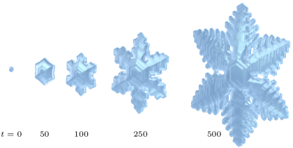
(a)   Fern dendrite 1

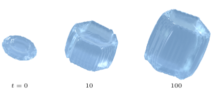
(b)   Hollow prism 1

Figure 1: Isosurface representation ($\phi=0$) of snowflake growth, using the software Blender for visual rendering. Top: fern dendrite 1. The growth mechanism is essentially two dimensional Libbrecht (2005). First, the initial disk grows into a transient flat faceted hexagon. Then, the branching instability occurs in the horizontal plane ($t=50$), for a critical crystal radius. The resulting faceted dendrites are equipped with developed faceted side branches. Bottom: prism 1. The seed grows vertically into a prism aligned on the Wulff shape. Then the basal facet breaks, and a hollow is formed at $t=10$. Time is indicated in $\tau_{0}$ unit.

For both cases, the growth stages are very similar to the experimental growth kinetics obtained by Libbrecht Libbrecht : the snowflake first aligns on the equilibrium Wulff shape, until the Mullins-Sekerka instability Mullins and Sekerka (1964) occurs for a critical crystal radius. This instability is related to the Berg effect Berg (1938), stating that the supersaturation field around a faceted snow crystal is largest at facet edges. Instability thus occurs when the snowflake reaches a critical radius Fujioka and Sekerka (1974), and kinetic effects at corners overcome the highly anisotropic surface tension Libbrecht (2005).

In Fig. 1(a), the simulated fernlike dendrite morphology differs from the non axisymmetric shape predicted by the theory of Brener Brener (1996), usually used to describe dendrites with cubic symmetry Singer and Bilgram (2004); Cartalade et al. (2016). We suggest this is due to the strong vertical anisotropy flattening, and to faceting, which limits the formation of a horizontal lacuna at the tail of dendrites. The obtained feathery shape with a transversally sharp tip rather resembles Furukawa’s experimental ice crystals Furukawa and Shimada (1993). Besides, experimental snowflakes display characteristic surface patterns, such as ridges Gravner and Griffeath (2009), and flat basal planes forming steps Furukawa and Shimada (1993). Such patterns are also reproduced by our model in Fig. 1(a). At low temperatures, surface nucleation and spiral growth are the leading growth processes on the basal faces for horizontal growth Nelson (2001). Though such mechanisms are not explicitly included in our model, the presence of surface steps in our simulations evokes the terrace growth resulting from nucleation, experimentally observed on ice crystals Sazaki et al. (2010). It can be underlined that the succession of flat basal planes on both real and simulated snowflakes, reflects the main stages of snowflake history. For instance, the hexagonal Wullf shape before branching instability is clearly memorized in Fig. 1(a). This is consistent with real snowflakes observation, provided in appendix A.

Fig. 2 displays the time evolution of snowflake size $L$, defined as the arm length for horizontal growth (blue), and the column length for vertical growth (red).

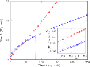
Figure 2: Snowflake size $L$ ($W_{0}$ units) vs. time $t$ ($\tau_{0}$ units) (marks), for $u_{0}=0.6$. Two growth regimes appear, with a transition at $t=50$ for vertical growth, and $t=80$ for horizontal growth (dots). First regime: $L(t)\propto t^{\alpha}$ ($\rho=0.99$), with $\alpha=0.62$ for horizontal growth (line), and $\alpha=0.63$ for vertical growth (dashes). Second regime: $L(t)\propto At$ ($\rho=0.99$), with $A=0.12$ for horizontal growth (line), and $A=0.41$ for vertical growth (dashes). Insert: tip velocity $V$ ($W_{0}/\tau_{0}$ units) vs. reduced supersaturation $u_{0}$ (marks). $V=A^{\prime}u_{0}$ ($\rho=0.99$) with $A^{\prime}=0.62$ for horizontal growth (line), and $A^{\prime}=0.62$ for vertical growth (dashes). Blue: horizontal growth (parameters 1 except $u_{0}$ varied from 0.2 to 0.6). Red: vertical growth (parameters 1 except $u_{0}$ varied from 0.2 to 0.6).

It can be seen that two growth regimes appear. After a first growth regime, when both dynamics are similar, the needle growth accelerates, while plate-like growth slows down. In the case of horizontal growth, Libbrecht experimentally noted in Libbrecht (2016), that this change of regime coincides with full faceting occurrence on the prismatic face, causing growth to decelerate. In the case of vertical growth, it was also observed in Libbrecht (2016), that the growth acceleration was related to the formation of a vicinal surface at the needle tip, which enhances water attachment at the tip. During the first regime, the crystal growth is slower than diffusion, and the system satisfies the Laplacian approximation. Within this framework, Algrem et al. found in Almgren et al. (1993), that arm growth should display the self similar scaling behaviour $L(t)\propto t^{3/5}$. This is confirmed by our simulations. It is interesting to note that the disparity of our simulations with the $t^{1/2}$ diffusive law of Zener et al. for spherical precipitates Zener (1949), is due to surface tension.

In the second regime, the growth kinetics is linear (line and dashes in Fig. 2), consistently with the selection theory Amar and Brener (1993); Saito (1996). The associated tip velocity $V$ is thus the slope of this linear function. Using the same procedure for different $u_{0}$, $V$ versus $u_{0}$ could be plotted in the insert. It appears that $V$ is proportional to $u_{0}$. Therefore, the growth velocity of both faceted and non faceted dendrites satisfies the universal law Langer et al. (1978).

$\Gamma<1$		$\Gamma\geq 1$
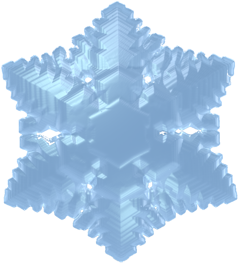
1 - stellar dendrite	1 - fern dendrite	1 - needle
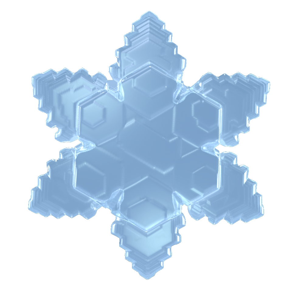
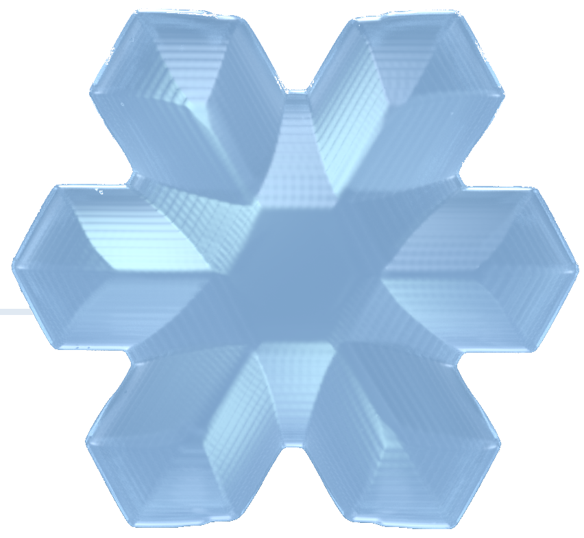
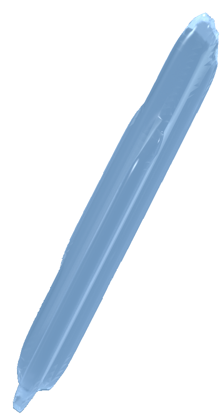
1 - dendrite plate	1 - stellar plate	1 needles cluster
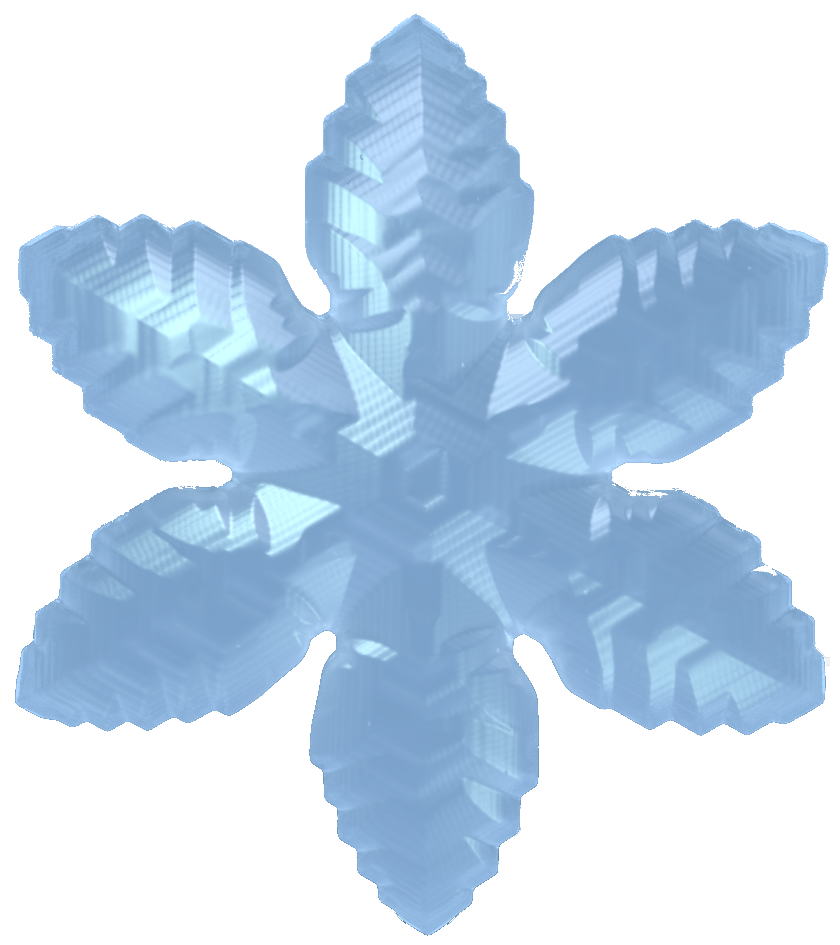
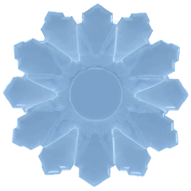
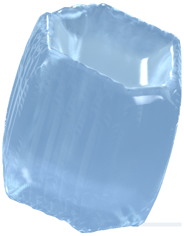
1 - simple star	1 - 12-star	1 - hollow prism
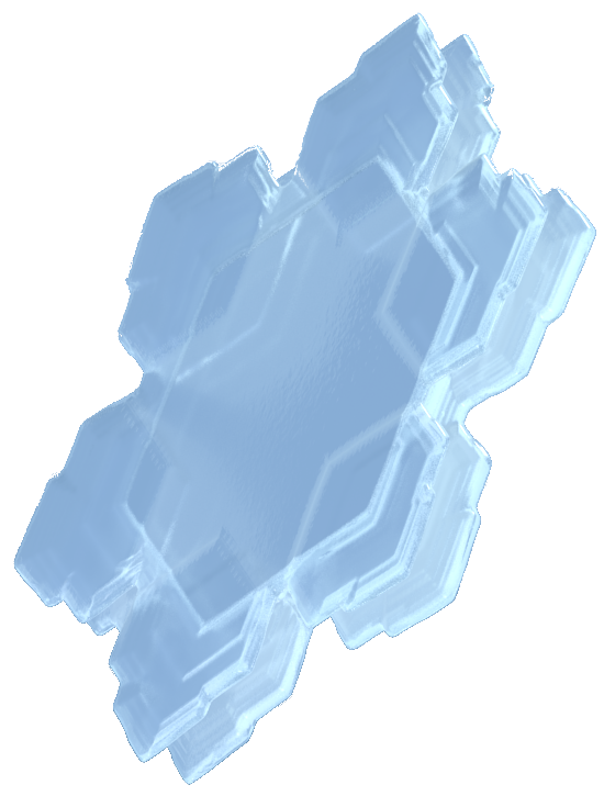
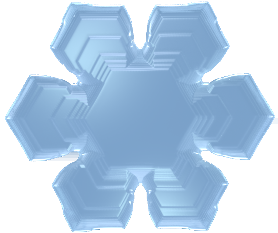
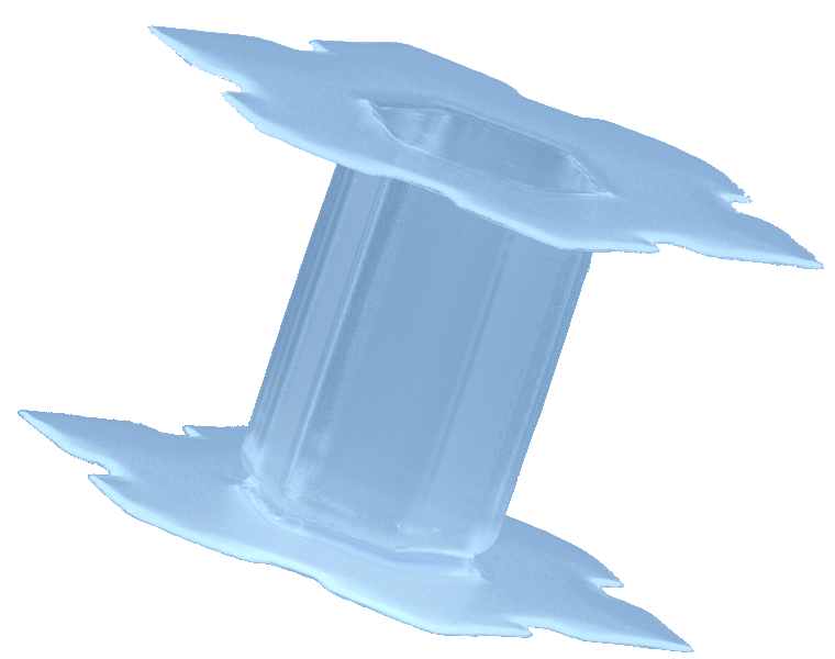
1 - double plate	1 - sectored plate	1 - capped col. a
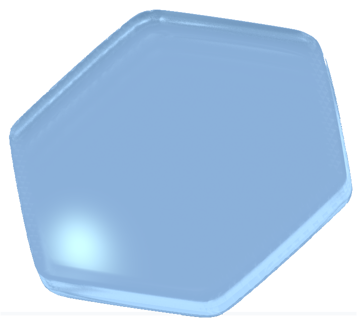
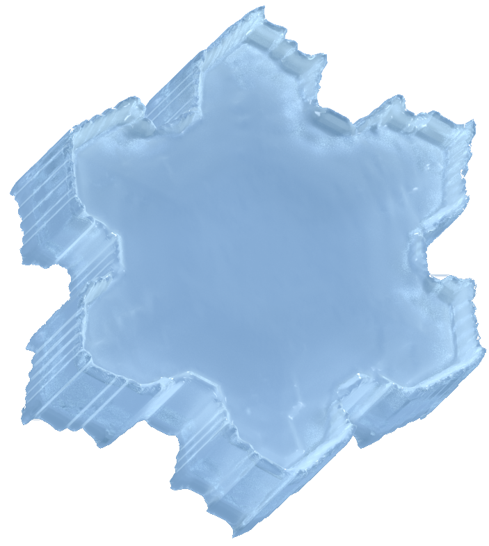
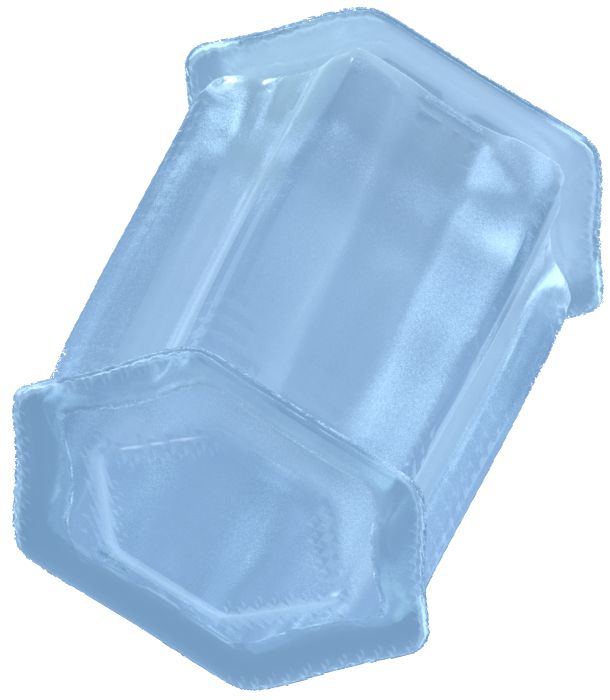
1 - solid plate	1 - scrolls on plate	1 - capped col. b

Figure 3: Simulated snowflake classification, using the software Blender for visual rendering. $\Gamma<1$ gives the flat snow crystals 1 to 1. $\Gamma\geq 1$ gives columns 1 & 1. Primary habit switch is achieved by shifting $\Gamma$ during simulations. $\Gamma$ from 3.0 to 0.2 at $t=70$, gives capped columns 1 and 1. $\Gamma$ from 0.4 to 3.0 gives scrolls on plate 1. For $\Gamma<1$, no facet breaking happens when $u_{0}\leq 0.4$ (solid plate 1). Branching instability appears for $u_{0}=0.5$ (snowflakes 1 to 1), and side branching requires $u_{0}\geq 0.7$ (dendrites 1 and 1). For $\Gamma>1$, $u_{0}=0.3$ gives a prism 1, and $u_{0}=0.8$ induces vertical branching with needles 1 and 1. $L_{\text{sat}}=1.0$ gives a thick side branching for the stellar dendrite 1. Rising $L_{\text{sat}}$ to $L_{\text{sat}}=1.6$ refines side branches with the fern dendrite 1. Higher values of $L_{\text{sat}}$ destroy side branching, and lead to branches maximum faceting with the stellar plate 1 ($L_{\text{sat}}=1.8$).

It is consistent with previous experimental Libbrecht et al. (2002), and numerical observations Debierre et al. (2003); Barrett et al. (2012). Langer et al. argued in Langer et al. (1978), that snowflake dendrites frontmost tip is molecularly rough for both non-faceted and faceted dendrites. The attachment kinetics can thus be considered isotropic with circular symmetry.

Fig. 3 compiles equilibrium shapes of simulated snowflakes, using the parameters in table 1. An achievement of our model is to recover the principal snowflake morphologies of the Nakaya diagram Nakaya (1951), depending exclusively on four parameters: $\Gamma$, $u_{0}$, $L_{\text{sat}}$ and $\epsilon_{z}$.

The first parameter $\Gamma$ fully determines the primary habit in our model. We suggest this parameter may be fitted on the yield between prismatic and basal attachment coefficients Libbrecht (2008). This yield accounts for the alternation of dominating growth mechanisms with the temperature. Two theories are proposed to explain this alternation of growth preference: surface nucleation for low temperatures Nelson (2001), and quasi-liquid layer growth causing surface roughening Kuroda and Lacmann (1982) near the melting point Libbrecht (2005). Then, Hertz-Knudsen relation for facet normal velocity Saito (1996) makes supersaturation $u_{0}$ the priming parameter in facet instability and growth velocity Nelson (2001). In the phase field model, the impact of $u_{0}$ is reinterpreted as the thermodynamic driving force, and higher values also favour branching instability and faster growth Singer-Loginova and Singer (2008). The parameter $L_{\text{sat}}$ controls the compactness of branching for non faceted growth Kobayashi (1993). Here, low values foster branching instability, while raising $L_{\text{sat}}$ drives the system toward quasistatic diffusion, and fosters a stronger faceting. As for the parameter $\epsilon_{z}$, it mainly influences the formation of surface patterns for horizontal growth.

Especially interesting are two model examples. First, the double plate 1 (p. 75 in Libbrecht (2006)), results from the sandwich instability of a flat snowflake, and the twelve arms star 1 was simulated by the aggregation of two simple stars, with a $30^{\circ}$ tilt Kikuchi and Uyeda (1998).

Finally, simulated snowflake morphology depends on temperature and density excess over vapour/water equilibrium $\rho_{\text{super}}^{W}=\rho-\rho_{\text{sat}}^{W}$ (g.m^-3). It is quantitatively consistent with the Nakaya diagram (see Marshall and Langleben (1954)). Using $u_{0}=(\rho_{\text{super}}^{W}+\rho_{\text{sat}}^{W}-\rho_{\text{sat}}^{I})/\rho_{\text{sat}}^{I}$, where $\rho_{\text{sat}}^{I}$ is the vapour/ice equilibrium density, and fitting $\Gamma$ on Libbrecht (2008), our simulations predict plate formation near $(T,\rho_{\text{super}}^{W})=(-19,0.15)$ and $(-12,0.4)$, versus $(-19,0.15)$, $(-12,0.4)$, but also $(-10,0.18)$ in the Nakaya diagram. Simulated dendrites occur near $(-16,0.4)$, versus $(-15,0.4)$ and $(-15,0.25)$ for experiments. Finally, hollow columns are formed at $(-8,0.6)$ in our simulations, versus $(-8,0.6)$ and $(-8,0.3)$ in the Nakaya diagram. However, small supersaturations $\rho_{\text{sat}}^{I}<\rho<\rho_{\text{sat}}^{W}$ are beyond reach for our model. This shortcoming is complementary to the model of Barrett et al. Barrett et al. (2012). Indeed, the latter is bound to $\rho\leq\rho_{\text{sat}}^{W}$ or $T\to 0^{\circ}$C, due to the Laplacian approximation for small supersaturations Libbrecht (2005). Our model on the contrary requires larger values for $L_{\text{sat}}$, and greater computational resources are needed to reach such supersaturations.

In this paper, we have shown that the proposed modified phase field model is able to reproduce the complex dynamics of snowflake growth. Benefiting from the modularity and versatility of the phase field model, this approach can be extended to describe the growth of snowflakes in the real atmospheric conditions. It can notably be equipped with stochastic effects, for the asymmetric growth of more exotic morphologies of snowflakes in the Nakaya diagram. Continuum fluid dynamics can also be easily introduced in the kinetics equation equation (1) and equation (2), to simulate the air flow around the snowflake during its fall from clouds Jeong et al. (2001). Besides, this approach is not restricted to snowflake growth. The developed approach opens a new way to answer numerous outstanding questions concerning dendritic growth in wide range of materials. We can cite, for instance, the faceted dendritic growth observed in pure isotactic polystyrene films, or the snowflake-like growth of graphene monocrystal Whiteway et al. (2015).

Author Contributions

G.D. and H.Z. developed the model and wrote the manuscript. R.P. participated in the code development. All authors analyzed the data, discussed the results and commented on the manuscript.

Appendix A comparison of simulations with real snowflakes

2

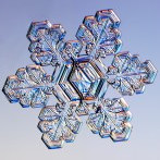
(a)   Simple star from Libbrecht

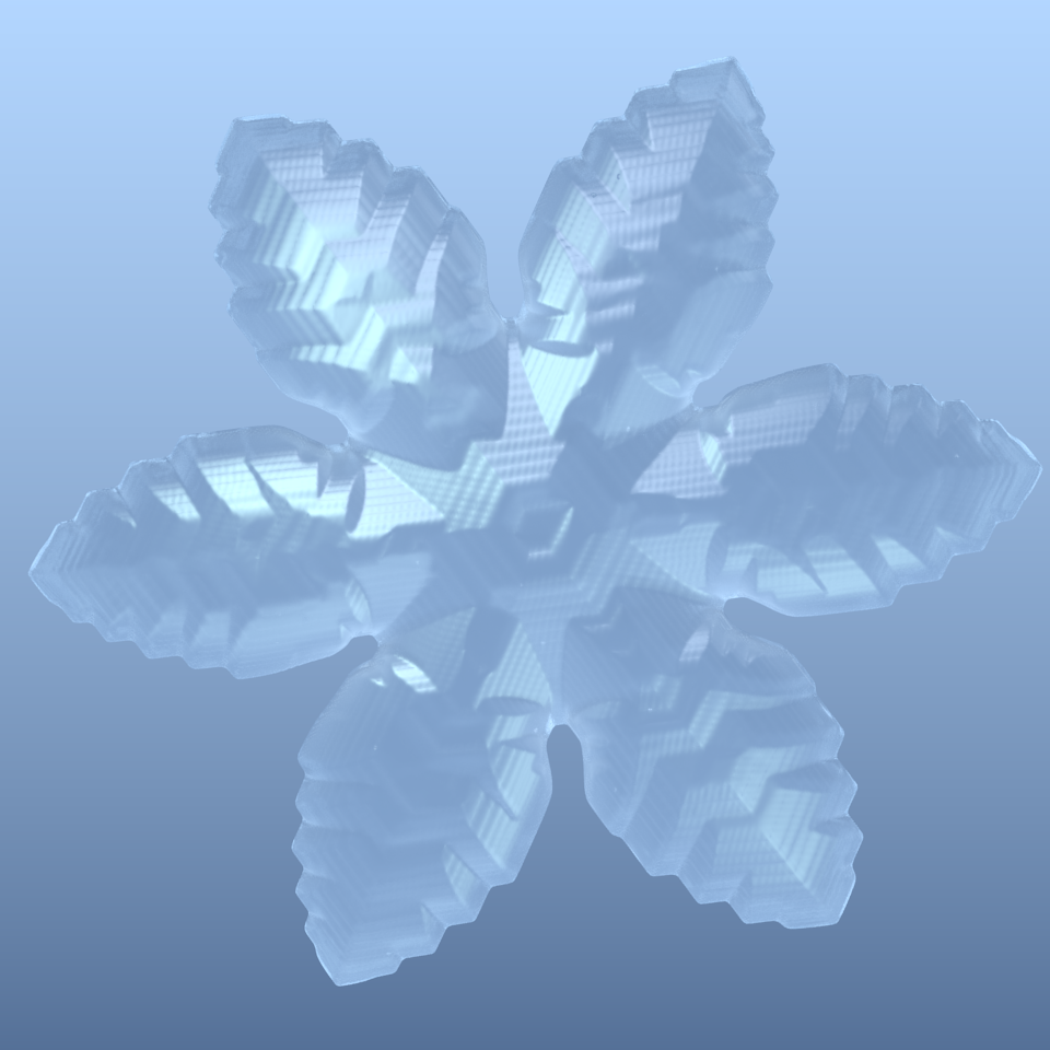
(b)   Simple star

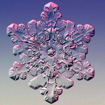
(c)   Stellar dendrite from Libbrecht

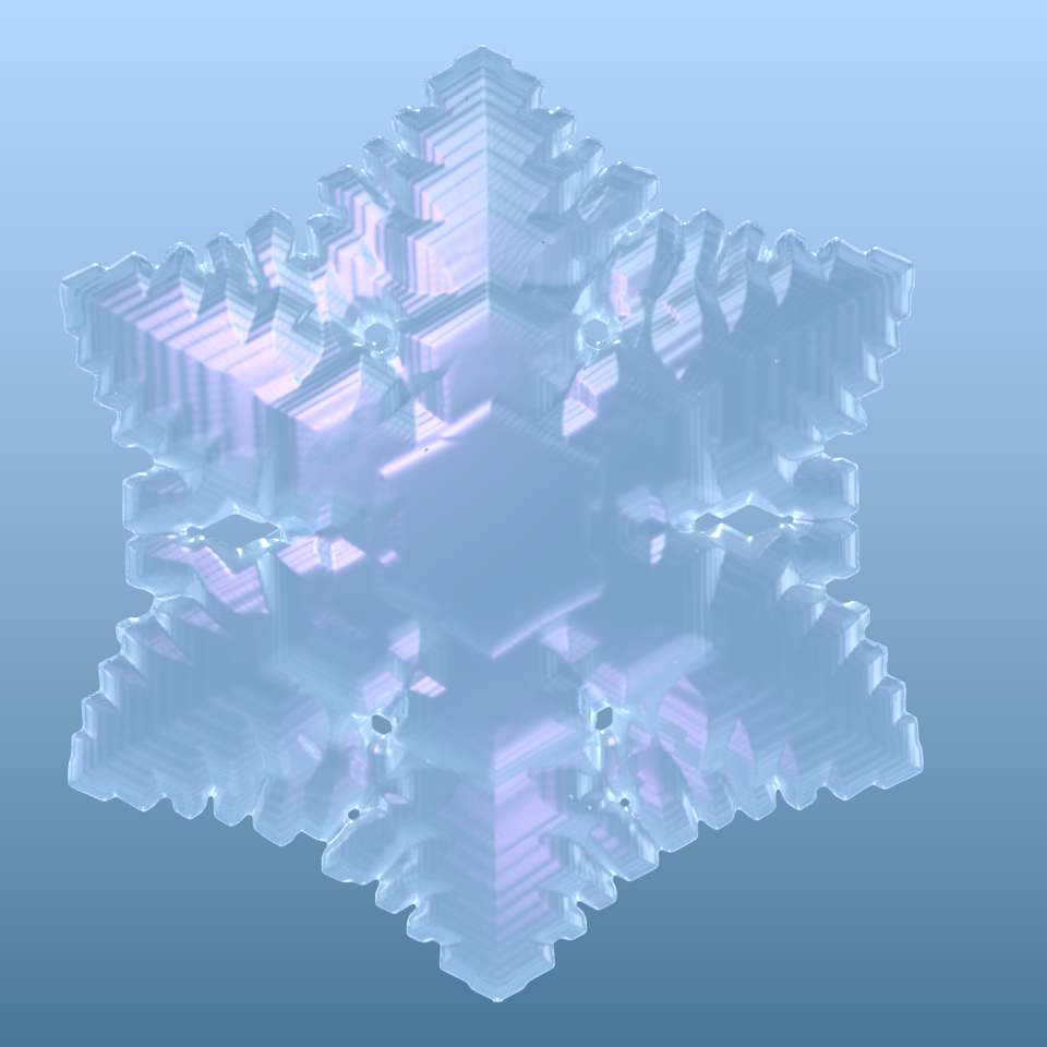
(d)   Stellar dendrite

(e)   Sectored plate from Libbrecht

(f)   Sectored plate

Figure 4: Comparison between real snowflakes photographs (left) taken from Libbrecht , and our phase field simulations (right). Visual rendering for our simulations uses the software Blender.

Appendix B simulation method

Phase field simulations were performed using the Fourier-spectral semi-implicit scheme with periodic boundary conditions. For horizontal growth, simulations were performed with grid spacing $\Delta x=\Delta y=\Delta z=0.8$, and time step $\Delta t=0.05$ Ramirez et al. (2004), on a 400 $\times$ 400 $\times$ 64 simulation box. Vertical growth simulations required a more precise discretization. Grid spacing was thus reduced to $\Delta x=\Delta y=\Delta z=0.4$, and $\Delta t=0.01$ as in Ramirez et al. (2004), on a 128 $\times$ 128 $\times$ 256 simulation box. Snow crystal growth was initiated by a circular-disk shape germ ($\phi=1$) of radius $R=8\Delta x$, within water vapour ($\phi=-1$) of homogeneous reduced supersaturation $u_{0}>0$. A new regularization method for high interfacial energy leading to crystal missing orientations was also adapted from two dimensions Eggleston et al. (2001), to three dimensions. This allowed to overcome the restriction for the critical values of the anisotropy constants and choose $\epsilon_{xy}>1/35$ and $\epsilon_{z}>1/3$, as required to achieve faceting Singer-Loginova and Singer (2008).

Appendix C 3D faceting algorithm

Faceting requires the anisotropy constants $\epsilon_{xy}$ and $\epsilon_{z}$ values in $A(\bm{n})$, to exceed $1/35$ for 6-fold horizontal symmetry, and $1/3$ for 2-fold vertical symmetry Singer-Loginova and Singer (2008). Above such values, metastable and unstable crystal orientations $\bm{n}$ where the stiffness becomes negative, emerge. $A(\bm{n})$ must hence be modified, so that the stiffness remains positive. A preliminary step is to determine missing orientations. This can be done by detecting sign change in the stiffness. This causes a local convexity inversion in the 2D polar plot of $1/A(\theta,\phi_{0})$, for any fixed azimuthal angle $\phi_{0}$, or in the polar plot of $1/A(\theta_{0},\phi)$ for any fixed polar angle $\theta_{0}$. This reads $A+\partial^{2}_{\theta\theta}A=0$ and $A+\partial^{2}_{\phi\phi}A=0$ respectively, providing us with the maximum anisotropy constants $\epsilon_{xy}^{m}$ and $\epsilon_{z}^{m}$ before missing orientation:

$$\left\{\begin{aligned} &\epsilon_{xy}^{m}=\frac{1+\epsilon_{z}\cos(2\phi)}{35}\\ &\epsilon_{z}^{m}=\frac{1+\epsilon_{xy}\cos(6\theta)}{3}.\end{aligned}\right.$$ (3)

Restricting the study to $\theta\in[-\pi/6,\pi/6]$ and $\phi\in[0,\pi]$ due to rotation periodicity of $A(\theta,\phi)$, missing $\theta$ orientations lie within a $\phi$-dependant angular sector $[-\theta^{m}(\phi)+k\pi/3,\theta^{m}(\phi)+k\pi/3]$ ($k\in\mathbb{Z}$) for $\epsilon_{xy}>\epsilon_{xy}^{m}$. Same goes for $\phi$ orientations lying within $[-\phi^{m}(\theta)+k\pi,\phi^{m}(\theta)+k\pi]$ for $\epsilon_{z}>\epsilon_{z}^{m}$. Following the procedure developed by Eggleston in Eggleston et al. (2001), $\theta^{m}$ and $\phi^{m}$ respectively satisfy $\partial_{\theta}[\cos(\theta)/A(\theta,\phi)]=0$ and $\partial_{\phi}[\cos(\phi)/A(\theta,\phi)]=0$, leading to:

$$\left\{\begin{aligned} &\frac{6\epsilon_{xy}\sin(6\theta^{m})\cos(\theta^{m})}{\sin(\theta^{m})}=\left(1+\epsilon_{xy}\cos(6\theta^{m})+\epsilon_{z}cos(2\phi)\right)\\ &\frac{2\epsilon_{z}\sin(2\phi^{m})\cos(\phi^{m})}{\sin(\phi^{m})}=\left(1+\epsilon_{xy}\cos(6\theta)+\epsilon_{z}cos(2\phi^{m})\right).\end{aligned}\right.$$ (4)

The regularization step finally consists in replacing $A(\theta,\phi)$ by a simple trigonometric function for missing orientation, as suggested by Debierre et al. Debierre et al. (2003):

$$A(\bm{n})=\left\{\begin{aligned} &A^{\theta}(\theta,\phi)=A_{1}(\phi)+B_{1}\cos(\theta),\text{ }|\theta|<\theta^{m},|\phi|\geq\phi^{m}\\ &A^{\phi}(\theta,\phi)=A_{2}(\theta)+B_{2}\cos(\phi),\text{ }|\theta|\geq\theta^{m},|\phi|<\phi^{m}\\ &\alpha(\theta,\phi)A^{\theta}+(1-\alpha(\theta,\phi))A^{\phi},\text{ }|\theta|<\theta^{m},|\phi|<\phi^{m}\\ &1+\epsilon_{xy}\cos(6\theta)+\epsilon_{z}\cos(2\psi)\text{ }\text{otherwise}.\end{aligned}\right.$$ (5)

Coefficients $A_{1}(\phi)$, $B_{1}$, $A_{2}(\theta)$, $B_{2}$ and $\alpha(\theta,\phi)$ are set to ensure continuity of $A(\bm{n})$ and its derivatives:

$$A_{1}(\phi)=1+\epsilon_{xy}\cos(6\theta^{m})+\epsilon_{z}\cos(2\phi)-\frac{6\epsilon_{xy}\sin(6\theta^{m})}{\sin(\theta^{m})}\cos(\theta^{m})$$ (6)

$$B_{1}=\frac{6\epsilon_{xy}\sin(6\theta^{m})}{\sin(\theta^{m})}$$

$$A_{2}(\theta)=1+\epsilon_{xy}\cos(6\theta)+\epsilon_{z}\cos(2\phi^{m})-\frac{2\epsilon_{z}\sin(2\phi^{m})}{\sin(\phi^{m})}\cos(\phi^{m})$$

$$B_{2}=\frac{2\epsilon_{z}\sin(2\phi^{m})}{\sin(\phi^{m})}$$

$$\alpha(\theta,\phi)=\frac{|\theta-\theta^{m}|}{\sqrt{(\theta-\theta^{m})^{2}+(\phi-\phi^{m})^{2}}}.$$

References

- Pamuk et al. (2012) B. Pamuk, J. M. Soler, R. Ramírez, C. P. Herrero, P. W. Stephens, P. B. Allen, and M.-V. Fernández-Serra, Phys. Rev. Lett. 108, 193003 (2012).
- Ball (2016) P. Ball, Nature Materials 15, 1060 (2016).
- Nakaya et al. (1938) U. Nakaya, I. Satô, and Y. Sekido, Journal of the Faculty of Science, Hokkaido Imperial University. Ser. 2 2, 1 (1938).
- Magono et al. (1966) C. Magono, W. Chung, et al., Journal of the Faculty of Science, Hokkaido University. Series 7, Geophysics 2, 321 (1966).
- Nakaya (1951) U. Nakaya, Compendium Meteor , 207 (1951).
- Libbrecht (2005) K. G. Libbrecht, Reports on progress in physics 68, 855 (2005).
- Mason (1992) B. J. Mason, Contemporary physics 33, 227 (1992).
- Kuroda and Lacmann (1982) T. Kuroda and R. Lacmann, Journal of Crystal Growth 56, 189 (1982).
- Nelson (2001) J. Nelson, Philosophical Magazine A 81, 2337 (2001).
- Nada and Furukawa (1996) H. Nada and Y. Furukawa, Journal of crystal growth 169, 587 (1996).
- Furukawa and Nada (1997) Y. Furukawa and H. Nada, The Journal of Physical Chemistry B 101, 6167 (1997).
- Benet et al. (2016) J. Benet, P. Llombart, E. Sanz, and L. G. MacDowell, Physical Review Letters 117, 096101 (2016).
- Gravner and Griffeath (2009) J. Gravner and D. Griffeath, Physical Review E 79, 011601 (2009).
- Barrett et al. (2012) J. W. Barrett, H. Garcke, and R. Nürnberg, Physical Review E 86, 011604 (2012).
- Libbrecht (2006) K. G. Libbrecht, Ken Libbrecht’s field guide to snowflakes (Voyageur Press, 2006).
- Furukawa and Shimada (1993) Y. Furukawa and W. Shimada, Journal of crystal growth 128, 234 (1993).
- Saito (1996) Y. Saito, Statistical physics of crystal growth, Vol. 2 (World Scientific, 1996).
- Sazaki et al. (2010) G. Sazaki, S. Zepeda, S. Nakatsubo, E. Yokoyama, and Y. Furukawa, Proceedings of the National Academy of Sciences 107, 19702 (2010).
- Kikuchi and Uyeda (1998) K. Kikuchi and H. Uyeda, Atmospheric Research 47–48, 169 (1998).
- Singer-Loginova and Singer (2008) I. Singer-Loginova and H. Singer, Reports on progress in physics 71, 106501 (2008).
- Karma and Rappel (1996) A. Karma and W.-J. Rappel, Physical Review E 53, R3017 (1996).
- Ramirez et al. (2004) J. Ramirez, C. Beckermann, A. Karma, and H.-J. Diepers, Physical Review E 69, 051607 (2004).
- Cartalade et al. (2016) A. Cartalade, A. Younsi, and M. Plapp, Computers & Mathematics with Applications 71, 1784 (2016).
- Barrett et al. (2013) J. W. Barrett, H. Garcke, and R. Nürnberg, ZAMM-Journal of Applied Mathematics and Mechanics/Zeitschrift für Angewandte Mathematik und Mechanik 93, 719 (2013).
- Kobayashi (1993) R. Kobayashi, Physica D: Nonlinear Phenomena 63, 410 (1993).
- Debierre et al. (2003) J.-M. Debierre, A. Karma, F. Celestini, and R. Guérin, Physical Review E 68, 041604 (2003).
- Eggleston et al. (2001) J. J. Eggleston, G. B. McFadden, and P. W. Voorhees, Physica D: Nonlinear Phenomena 150, 91 (2001).
- Libbrecht (2012) K. G. Libbrecht, arXiv preprint arXiv:1211.5555 (2012).
- Langer et al. (1978) J. Langer, R. Sekerka, and T. Fujioka, Journal of Crystal Growth 44, 414 (1978).
- Langer and Müller-Krumbhaar (1978) J. Langer and H. Müller-Krumbhaar, Acta Metallurgica 26, 1681 (1978).
- Amar and Brener (1993) M. B. Amar and E. Brener, Physical review letters 71, 589 (1993).
- Brener (1996) E. Brener, Journal of crystal growth 166, 339 (1996).
- Libbrecht et al. (2002) K. G. Libbrecht, T. Crosby, and M. Swanson, Journal of crystal growth 240, 241 (2002).
- (34) K. G. Libbrecht, “Snowcrystals.com,” http://www.snowcrystals.com.
- Mullins and Sekerka (1964) W. W. Mullins and R. Sekerka, Journal of applied physics 35, 444 (1964).
- Berg (1938) W. Berg, in Proceedings of the Royal Society of London A: Mathematical, Physical and Engineering Sciences, Vol. 164 (The Royal Society, 1938) pp. 79–95.
- Fujioka and Sekerka (1974) T. Fujioka and R. Sekerka, Journal of Crystal Growth 24, 84 (1974).
- Singer and Bilgram (2004) H. Singer and J. Bilgram, EPL (Europhysics Letters) 68, 240 (2004).
- Libbrecht (2016) K. G. Libbrecht, arXiv preprint arXiv:1602.08528 (2016).
- Almgren et al. (1993) R. Almgren, W.-S. Dai, and V. Hakim, Physical review letters 71, 3461 (1993).
- Zener (1949) C. Zener, Journal of Applied Physics 20, 950 (1949).
- Libbrecht (2008) K. G. Libbrecht, arXiv preprint arXiv:0810.0689 (2008).
- Marshall and Langleben (1954) J. S. Marshall and M. P. Langleben, Journal of Meteorology 11, 104 (1954).
- Jeong et al. (2001) J.-H. Jeong, N. Goldenfeld, and J. A. Dantzig, Phys. Rev. E 64, 041602 (2001).
- Whiteway et al. (2015) E. Whiteway, W. Yang, V. Yu, and M. Hilke, arXiv preprint arXiv:1509.01579 (2015).