Prediction Accuracy Measures for a Nonlinear Model and for Right-Censored Time-to-Event Data

Abstract

This paper studies prediction summary measures for a prediction function under a general setting in which the model is allowed to be misspecified and the prediction function is not required to be the conditional mean response. We show that the $R^{2}$ measure based on a variance decomposition is insufficient to summarize the predictive power of a nonlinear prediction function. By deriving a prediction error decomposition, we introduce an additional measure, $L^{2}$, to augment the $R^{2}$ measure. When used together, the two measures provide a complete summary of the predictive power of a prediction function. Furthermore, we extend these measures to right-censored time-to-event data by establishing right-censored data analogs of the variance and prediction error decompositions. We illustrate the usefulness of the proposed measures with simulations and real data examples. Supplementary materials for this article are available online.

Keywords: Accelerated Failure Time Model; Censoring; Multiple Correlation Coefficient; Coefficient of Determination; Cox’s Proportional Hazards Model; Nonlinear Model; Prediction; R-Squared Statistic.

1 Introduction

In this paper we develop prediction accuracy ymeasures for a nonlinear model and for right-censored time-to-event data. In addition to evaluating a model’s prediction performance, prediction Accuracymeasures are useful for assessing the practical importance of predictors and for comparing competing models that are not necessarily nested nor correctly specified.

By far, the most commonly used prediction accuracy measure for a linear model is the R-squared statistic, or coefficient of determination. Let $Y$ be a real-valued random variable and $X$ be a vector of $p$ real-valued explanatory random variables or covariates. Assume that one observes a random sample $(Y_{1},X_{1}),\ldots,(Y_{n},X_{n})$ from the distribution of $(Y,X)$. The R-squared statistic is defined as

$$R^{2}=1-\frac{\sum_{i=1}^{n}(Y_{i}-\hat{Y}_{i})^{2}}{\sum_{i=1}^{n}(Y_{i}-\bar{Y})^{2}},$$ (1)

where $\hat{Y}_{i}=a+b^{T}X_{i}$ is the least squares predicted value for subject $i$. The $R^{2}$ statistic has the straightforward interpretation as the proportion of variation of $Y$ which is explained by the least squares prediction function due to the following decomposition:

$$\sum_{i=1}^{n}(Y_{i}-\bar{Y})^{2} = \sum_{i=1}^{n}(\hat{Y}_{i}-\bar{Y})^{2}+\sum_{i=1}^{n}(Y_{i}-\hat{Y}_{i})^{2}.$$ (2)

total variation $$= \mbox{explained variation }+\mbox{ unexplained variation }$$

Despite its popularity in linear regression, the $R^{2}$ statistic defined by (1) is not readily applicable to a nonlinear model since the decomposition (2) no longer holds. In the past decades, much efforts have been devoted to extending the R-squared statistic to nonlinear models. Among others, the pseuodo $R^{2}$ statistics for a nonlinear model include likelihood-based measures (Goodman, 1971; McFadden et al., 1973; Maddala, 1986; Cox and Snell, 1989; Magee, 1990; Nagelkerke, 1991), information-based measures (McFadden et al., 1973; Kent, 1983), ranking-based measures (Harrell et al., 1982), variation-based measures (Theil, 1970; Efron, 1978; Haberman, 1982; Hilden, 1991; Cox and Wermuth, 1992; Ash and Shwartz, 1999), and the multiple correlation coefficient measure (Mittlböck et al., 1996; Zheng and Agresti, 2000). However, none of the existing pseudo $R^{2}$ measures are motivated directly from a variance decomposition and none have received the same widespread acceptance as the classical $R^{2}$ for linear regression. Interested readers are referred to Zheng and Agresti (2000) for an excellent survey of existing pseudo $R^{2}$ measures and further references on this topic.

The first goal of this paper is to develop prediction accuracy measures for a prediction function under a general setting in which the model is allowed to be misspecified and the prediction function may be different from the conditional expected response. We begin with defining population prediction accuracy measures. Based on a simple variance decomposition, we define a $\rho^{2}$ measure as the proportion of the explained variance of $Y$ by a corrected prediction function. It can be shown that the $\rho^{2}$ parameter is identical to the squared multiple correlation coefficient between the response and the predicted response. Since it describes the proportion of the explained variance by the corrected prediction function, which in general is not the same as the uncorrected prediction functions, the squared multiple correlation coefficient, a popular pseudo $R^{2}$, is not sufficient to summarize the predictive power of nonlinear models. As a remedy, we derive another parameter, named $\lambda^{2}$, as the proportion of the explained prediction error by the corrected prediction function based on a mean-squared prediction error decomposition. The parameter $\lambda^{2}$ measures how close the uncorrected prediction function is to its corrected version. The two parameters characterize complementary aspects regarding the predictive accuracy of the prediction function. When used in combination, they provide a complete summary of the predictive power of the uncorrected prediction function. We further obtain finite sample versions of the variance and prediction error decompositions, define the corresponding sample prediction accuracy measures, namely $R^{2}$ and $L^{2}$, and establish their asymptotic properties. It is worth noting that for the least squares prediction function under the linear model, the $L^{2}$ measure degenerates to 1 and therefore only $R^{2}$ is needed to describe its predictive power in the classical linear regression analysis.

The second goal of the paper is to develop new prediction accuracy measures for an event time model based on right censored time-to-event data. Note that it is challenging to extend the $R^{2}$ definition (1) to right-censored data even for the linear model. A variety of pseudo $R^{2}$ measures and other loss functions have been proposed for event time models with right-censored data (Kent and O’QUIGLEY, 1988; Korn and Simon, 1990; Graf et al., 1999; Schemper and Henderson, 2000; Royston and Sauerbrei, 2004; O’Quigley et al., 2005; Stare et al., 2011). For example, the EV option in the SAS PHREG procedure gives a generalized $R^{2}$ measure proposed by Schemper and Henderson (2000) for Cox’s (1972) proportional hazards model. A more recent proposal by Stare et al. (2011) uses explained rank information, which is applicable to a wide range of event time models. Stare et al. (2011) also gave a thorough literature review of prediction accuracy measures for event time models. We highlight that for linear regression, none of the existing pseudo $R^{2}$ measures for right censored data reduce to the classical R-squared statistic in the absence of censoring. Moreover, under a correctly specified model, they do not converge to the nonparametric population R-squared value $\rho_{NP}^{2}\equiv var{(E(Y|X))}/var(Y)$, the proportion of the explained variance by $E(Y|X)$, as the sample size grows large. Finally, as shown in Section 4 (Table 1) that the pseudo $R^{2}$ measures of Schemper and Henderson (2000); Stare et al. (2011) are not suitable for comparing unnested Cox’s models with possibly different baseline hazards and could remain constant when the nonparametric population R-squared value $\rho_{NP}^{2}$ varies from 0 to 1. In this paper, we derive a variance and a prediction error decomposition for right censored data. These decompositions allows us to define a pair of prediction accuracy measures, $R^{2}$ and $L^{2}$, for an event time model with right-censored data in exactly the same way as uncensored data. The proposed measures possess many appealing properties that most existing pseudo $R^{2}$ measures do not have. First, for the linear model with no censoring, our $R^{2}$ statistic reduces to the classical coefficient of determination and $L^{2}$ reduces to 1. Second, when the prediction is the conditional mean response based on a correctly specified model, our $R^{2}$ statistic is a consistent estimate of the nonparametric coefficient of determination $\rho_{NP}^{2}$, and $L^{2}$ converges to 1 as the sample size grows large. Third, our method is applicable to any event time model with right-censored data. Fourth, our measures are defined without requiring the model to be correctly specified. Lastly, our measures can be used to compare unnested models.

The rest of the paper is organized as follows. In Section 2.1, we define a pair of population prediction accuracy measures for a general prediction function from a possibly mis-specified model by deriving a variance decomposition and a mean squared prediction error decomposition. Sample measures based on independent and identically distributed complete data are then proposed and studied in Section 2.2. Section 3 discusses how to extend these measures to event time models with right-censored data. Section 4 presents simulation studies to illustrate the performance of the proposed sample measures and compare them with some existing measures in the literature. Real data illustrations are given in Section 5. Proofs of theoretical results are deferred to Appendix. Final remarks are provided in Section 6.

2 Prediction Summary Measures for a Nonlinear Model

Denote by $F(y|x)=P(Y\leq y|X=x)$ and $\mu(x)=E(Y|X=x)$ the true conditional distribution function and the true conditional expectation of $Y$ given $X=x$, respectively.

Consider a regression model of $Y$ on $X$ described by a family of conditional distribution functions ${\cal M}=\{F_{\theta}(y|x):\theta\in\Theta\}$, where the parameter $\theta$ is either finite dimensional or infinite dimensional. For example, $F_{\theta}(y|x)=\Phi((y-\alpha-\beta^{T}x)/\sigma)$ for the linear regression model with a normal $N(0,\sigma^{2})$ random error, where $\theta=(\alpha,\beta^{T},\sigma^{2})$ and $\Phi$ is the standard normal cumulative distribution function. The Cox (1972) proportional hazards model is an example of a semi-parametric regression model with $F_{\theta}(y|x)=1-\{1-F_{0}(y)\}^{\exp(\beta^{T}x)}$ where $\theta=(\beta,F_{0})$ consists of a finite dimensional regression parameter $\beta$ and an infinite dimensional unknown baseline distribution function $F_{0}$. We allow the model ${\cal M}$ to be misspecified in the sense that ${\cal M}$ may not include the true conditional distribution function $F(y|x)$ as a member.

For any $\theta\in\Theta$, let $m_{\theta}(X)$ be a prediction function of $Y$ obtained as a functional of $F_{\theta}(\cdot|X)$. Common examples of $m_{\theta}(X)$ include the conditional mean response defined by $m_{\theta}(x)=\int ydF_{\theta}(y|x)$ and the conditional median response $m_{\theta}(x)=F^{-1}_{\theta}(0.5|x)$. Assume that $\hat{\theta}$ is a sample statistic such that as $n\to\infty$,

$$\hat{\theta}\buildrel P\over{\longrightarrow}\theta^{*},\quad\mbox{for some $\theta^{*}\in\Theta$. }$$ (3)

For example, if $\hat{\theta}$ is the maximum likelihood estimate for a parametric model, then under some regularity conditions $\hat{\theta}$ converges in probability to a well-defined limit, $\theta^{*}$, even when the model is misspecified (Huber, 1967). If the model is correctly specified, then $\theta^{*}$ is the true parameter value. On the other hand, if the model is misspecified, then $\theta^{*}$ is the parameter that minimizes the Kullback-Leibler Information Criterion (Akaike, 1998).

In this section, we first develop population prediction accuracy measures for $m_{\theta^{*}}(X)$, which can be regarded as the asymptotic accuracy measures for the predictive power of $m_{\hat{\theta}}(x)$. Sample prediction accuracy measures for $m_{\hat{\theta}}(X)$ are then derived accordingly and their asymptotic properties are studied.

2.1 Population Prediction Summary Measures

For any $p$-variate function $P(x)$, define

$$MSPE(P(X))=E\{Y-P(X)\}^{2}.$$

as the mean squared prediction error ($MSPE$) of $P(X)$ for predicting $Y$.

In general, one would expect a good prediction function $P(X)$ of $Y$ to possess at least the following basic properties: i) $E\{P(X)\}=\mu_{Y}$, and ii) $MSPE(P(X))\leq MSPE(\mu_{Y})$, where $\mu_{Y}=E(Y)$ is the best prediction among all constant (non-informative) predictions of $Y$ as measured by $MSPE$. However, such minimal requirements are not always satisfied by $m_{\theta^{*}}(X)$ when the model ${\cal M}$ is possibly misspecified or when the prediction is not based on the conditional mean response. Below we introduce a linear correction of $m_{\theta^{*}}(X)$ so that the corrected prediction function always satisfies these minimal requirements.

Definition 2.1

The linearly corrected prediction function of $m_{\theta^{*}}(X)$ is defined as

$$m_{\theta^{*}}^{(c)}(X)=\mu_{Y}+\frac{cov(Y,m_{\theta^{*}}(X))}{var(m_{\theta^{*}}(X))}[m_{\theta^{*}}(X)-E\{m_{\theta^{*}}(X)\}].$$ (4)

It is straightforward to show that $m_{\theta^{*}}^{(c)}(X)$ has the following properties.

1. $m_{\theta^{*}}^{(c)}(X)=\tilde{a}+\tilde{b}m_{\theta^{*}}(X)$, where $(\tilde{a},\tilde{b})=\arg\min_{\alpha,\beta}E\{Y-(\alpha+\beta m_{\theta^{*}}(X))\}^{2}$;

2. $E(m_{\theta^{*}}^{(c)}(X))=\mu_{Y}$;

3. $MPSE(m_{\theta^{*}}^{(c)}(X))\leq MPSE(\mu_{Y})$;

4. $MPSE(m_{\theta^{*}}^{(c)}(X))\leq MPSE(m_{\theta^{*}}(X))$.

It follows from (i) and (ii) that $m_{\theta^{*}}^{(c)}(X)$ is the best unbiased prediction of $Y$ among all linear functions of $m_{\theta^{*}}(X)$. Moreover, the corrected function facilitates two elementary decompositions as stated in Lemma  2.1 below.

Lemma 2.1

Let $m_{\theta^{*}}^{(c)}(X)$ be the corrected prediction function of $m_{\theta^{*}}(X)$ defined by (4). Then,

1. (Variance decomposition)

   $$var(Y) = E\{m_{\theta^{*}}^{(c)}(X)-\mu_{Y}\}^{2}+E\{Y-m_{\theta^{*}}^{(c)}(X)\}^{2},$$

   $$= \mbox{explained variance}+\mbox{unexplained variance}$$

   where the first and second terms on the right hand side represent respectively the explained variance and the unexplained variance of $Y$ by $m_{\theta^{*}}^{(c)}(X)$.

2. (Prediction Error Decomposition)

   $$MSPE(m_{\theta^{*}}(X)) = E\{Y-m_{\theta^{*}}^{(c)}(X)\}^{2}+E\{m_{\theta^{*}}^{(c)}(X)-m_{\theta^{*}}(X)\}^{2}$$

   $$= \mbox{explained prediction error}+\mbox{ unexplained prediction error }$$

   where the first and second terms on the right hand side can be interpreted as the explained prediction error and unexplained prediction error of $m_{\theta^{*}}(X)$ by $m_{\theta^{*}}^{(c)}(X)$.

Based on the above decompositions, we introduce the following prediction accuracy measures.

Definition 2.2

Define

$$\rho^{2}_{m_{\theta^{*}}} = 1-\frac{E\{Y-m_{\theta^{*}}^{(c)}(X)\}^{2}}{var(Y)}=\frac{E\{m_{\theta^{*}}^{(c)}(X)-\mu_{Y}\}^{2}}{var(Y)},$$ (7)

to be the proportion of the variance of $Y$ that is explained by $m_{\theta^{*}}^{(c)}(X)$, and

$$\lambda^{2}_{m_{\theta^{*}}} = \frac{MSPE(m_{\theta^{*}}^{(c)}(X))\}^{2}}{MSPE(m_{\theta^{*}}(X))}=1-\frac{E\{m_{\theta^{*}}^{(c)}(X)-m_{\theta^{*}}(X)\}^{2}}{MSPE(m_{\theta^{*}}(X))}.$$ (8)

to be the proportion of the $MSPE$ of $m_{\theta^{*}}(X)$ that is explained by $m_{\theta^{*}}^{(c)}(X)$.

Remark 2.1

The parameters $\rho^{2}_{m_{\theta^{*}}}$ and $\lambda^{2}_{m_{\theta^{*}}}$ measure two distinct, yet complementary aspects regarding the prediction accuracy of $m_{\theta^{*}}(X)$: $\rho^{2}_{m_{\theta^{*}}}$ measures the predictive power of the corrected prediction function $m_{\theta^{*}}^{(c)}(X)$, whereas $\lambda^{2}_{m_{\theta^{*}}}$ measures how close $m_{\theta^{*}}(X)$ is to $m_{\theta^{*}}^{(c)}(X)$. When used together, they provide a complete accuracy of the predictive power of the uncorrected prediction function $m_{\theta^{*}}(X)$. Note that $0\leq\rho^{2}_{m_{\theta^{*}}}\leq 1$ and $0\leq\lambda_{m_{\theta^{*}}}^{2}\leq 1$. Moreover, $\rho^{2}_{m_{\theta^{*}}}=1$ and $\lambda^{2}_{m_{\theta^{*}}}=1$ if and only if $m_{\theta^{*}}(X)=Y$ with probability 1. So $m_{\theta^{*}}(X)$ has high predictive power if both measures are close to 1. If $\rho^{2}_{m_{\theta^{*}}}$ is large, but $\lambda^{2}_{m_{\theta^{*}}}$ is small, then $m_{\theta^{*}}(X)$ does not have good predictive power even though the corrected prediction $m_{\theta^{*}}^{(c)}(X)$ does. Lastly, if $\rho^{2}_{m_{\theta^{*}}}$ is small, then $m_{\theta^{*}}^{(c)}(X)$ and consequently $m_{\theta^{*}}(X)$ both do not have good prediction power regardless the magnitude of $\lambda^{2}_{m_{\theta^{*}}}$.

Remark 2.2

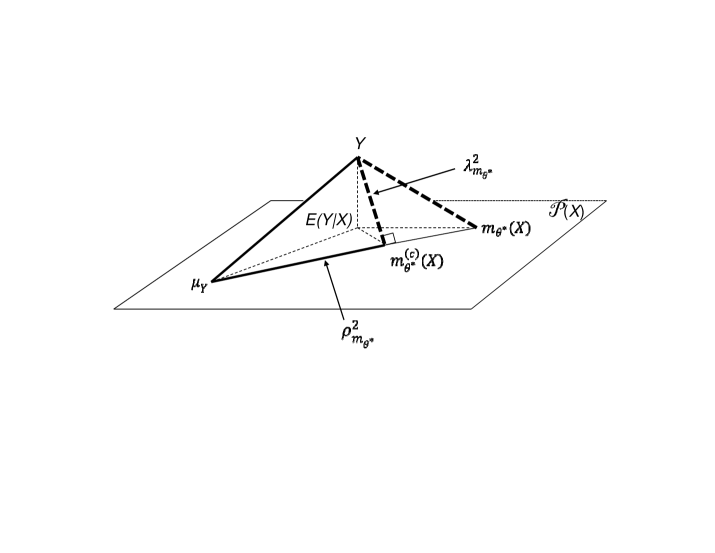
Figure 1: Geometric interpretation of $\rho^{2}_{m_{\theta^{*}}}$ and $\lambda^{2}_{m_{\theta^{*}}}$

(Geometric Interpretation). One may gain more insight about these parameters by examining the geometric relationship between the related quantities. Define the $L_{2}$-distance between any two real-valued random variables $\xi$ and $\eta$ by $d_{2}(\xi,\eta)=\left\{E(\xi-\eta)^{2}\right\}^{\frac{1}{2}}.$ The geometric relationship between $Y$, $\mu_{Y}$, $m_{\theta^{*}}(X)$, $m_{\theta^{*}}^{(c)}(X)$, and $\mu(X)$ are depicted in Figure 1, in which ${\cal P}(X)$ denotes the space of all real-valued functions of $X$.

[Insert Figure 1 approximately here]

As illustrated in Figure 1, $m_{\theta^{*}}^{(c)}(X)$ is the projection of $Y$ onto the subspace of all linear functions of $m_{\theta^{*}}(X)$ and $\mu(X)$ is the projection of $Y$ onto ${\cal P}(X)$. The variance decomposition in Lemma 2.1(a) corresponds to the Pythagorean theorem for the triangle $(Y,m_{\theta^{*}}^{(c)}(X),\mu_{Y})$ that leads to the definition of $\rho^{2}_{m_{\theta^{*}}}$. The prediction error decomposition is the Pythagorean theorem for the triangle $(Y,m_{\theta^{*}}^{(c)}(X),m_{\theta^{*}}(X))$ that defines $\lambda^{2}_{m_{\theta^{*}}}$.

Remark 2.3

(Interpretation of $\lambda_{m_{\theta^{*}}}^{2}$ as a measure of the prediction bias for the mean regression function $\mu(X)$). Assume that $m_{\theta^{*}}(X)$ is a nonlinear prediction function. It is easily seen that if $m_{\theta^{*}}(X)=\mu(X)$, then $\lambda^{2}_{m_{\theta^{*}}}=1$. Thus, $\lambda^{2}_{m_{\theta^{*}}}<1$ implies that $m_{\theta^{*}}(X)\neq\mu(X)$. In particular, if $m_{\theta^{*}}(X)$ is the conditional mean response under model ${\cal M}$, then $\lambda^{2}_{m_{\theta^{*}}}<1$ implies that the model is mis-specified.

It is also seen from Figure 1 that the Pythagorean theorem for the triangle $(Y,\mu(X),\mu_{Y})$ corresponds to the well known variance decomposition

$$var(Y) = var(\mu(X))+E(var(Y|X))$$

$$= \mbox{explained variance by $\mu(X)$}+\mbox{ unexplained variance}.$$

We refer the proportion of explained variance by $\mu(X)$:

$$\rho^{2}_{NP}\equiv 1-\frac{E(Y-\mu(X))^{2}}{var(Y)}=\frac{var(\mu(X))}{var(Y)},$$ (9)

as the nonparametric coefficient of determination. Note that $\rho_{NP}$ is the “correlation ratio” studied previously by Rényi (1959).

The next theorem summarizes some fundamental properties of $\rho^{2}_{m_{\theta^{*}}}$ and $\lambda^{2}_{m_{\theta^{*}}}$.

Theorem 2.1

1. Let $\rho(\xi,\eta)$ denote the correlation coefficient between two random variables $\xi$ and $\eta$. Then, $\rho^{2}_{m_{\theta^{*}}}=[\rho(Y,m_{\theta^{*}}(X))]^{2}$;

2. (Linear Prediction). Let $BLUE(X)=a+b^{T}X$ be the best linear unbiased estimator (BLUE) of $Y$, where $(a,b)=\arg\min_{\alpha,\beta}E\{Y-(\alpha+\beta^{T}X)\}^{2}$. Then (i) $BLUE^{(c)}(X)=BLUE(X)$; (ii) ${\lambda^{2}_{BLUE}}\equiv 1$; (iii) $\rho^{2}_{BLUE}$ is equal to the population value of the classical coefficient of determination for linear regression.

3. If $m_{\theta^{*}}(X)=\mu(X)$, then $\lambda_{m_{\theta^{*}}}^{2}\equiv 1$, and $\rho^{2}_{m_{\theta^{*}}}=\rho^{2}_{NP}$, where $\rho^{2}_{NP}$ is the nonparametric coefficient of determination defined by (9);

4. (Maximal $\rho^{2}$). Let $\rho^{2}_{NP}$ be defined by (9). Then

   $$\rho_{NP}^{2}=\max_{Q\in{\cal P}(X)}\{\rho^{2}_{Q}\}$$

   where ${\cal P}(X)$ is the space of all $p$-variate functions $Q(X)$ of $X$. In other words, $\rho^{2}_{NP}$ is the maximal coefficient of determination over all prediction functions $Q(X)$.

2.2 Sample Prediction Summary Measures

Assume that one observes a random sample $(Y_{1},X_{1}),\ldots,(Y_{n},X_{n})$ of $n$ independent and identically distributed (i.i.d.) replicates of $(Y,X)$. Now we derive sample accuracy measures for the predictive power of $m_{\hat{\theta}}(X)$, where $\hat{\theta}=\hat{\theta}(Y_{1},X_{1},\ldots,Y_{n},X_{n})$ is a sample statistic satisfying (3).

We first give a finite sample version of the decompositions in Lemma 2.1.

Lemma 2.2

Define

$$m^{(c)}_{\hat{\theta}}(x)=\hat{a}+\hat{b}m_{\hat{\theta}}(x),$$ (10)

to be the linearly corrected function for $m_{\hat{\theta}}(x)$, where $\hat{a}=\bar{Y}-\hat{b}\bar{m}_{\hat{\theta}},\hat{b}=\frac{\sum_{i=1}^{n}(Y_{i}-\bar{Y})\{m_{\hat{\theta}}(X_{i})-\bar{m}_{\hat{\theta}}\}}{\sum_{i=1}^{n}\{m_{\hat{\theta}}(X_{i})-\bar{m}_{\hat{\theta}}\}^{2}},$ ${\bar{Y}}=n^{-1}\sum_{i=1}^{n}Y_{i},$ and $\bar{m}_{\hat{\theta}}=n^{-1}\sum_{i=1}^{n}m_{\hat{\theta}}(X_{i})$. In other words, $m^{(c)}_{\hat{\theta}}(x)$ is the ordinary least squares regression function obtained by linearly regressing $Y_{1},\ldots,Y_{n}$ on $m_{\hat{\theta}}(X_{1}),\dots,m_{\hat{\theta}}(X_{n})$. Then

1. (Variance Decomposition)

   $$\sum_{i=1}^{n}(Y_{i}-{\bar{Y}})^{2}=\sum_{i=1}^{n}(m^{(c)}_{\hat{\theta}}(X_{i})-\bar{Y})^{2}+\sum_{i=1}^{n}(Y_{i}-m^{(c)}_{\hat{\theta}}(X_{i}))^{2};$$ (11)

2. (Prediction Error Decomposition)

   $$\sum_{i=1}^{n}(Y_{i}-m_{\hat{\theta}}(X_{i}))^{2}=\sum_{i=1}^{n}(Y_{i}-m^{(c)}_{\hat{\theta}}(X_{i}))^{2}+\sum_{i=1}^{n}(m^{(c)}_{\hat{\theta}}(X_{i})-m_{\hat{\theta}}(X_{i}))^{2}.$$ (12)

The sample version of $\rho^{2}$ and $\lambda^{2}$ are then defined by

$$R^{2}_{m_{\hat{\theta}}}=\frac{\sum_{i=1}^{n}(m^{(c)}_{\hat{\theta}}(X_{i})-\bar{Y})^{2}}{\sum_{i=1}^{n}(Y_{i}-{\bar{Y}})^{2}},$$ (13)

and

$$L^{2}_{m_{\hat{\theta}}}=\frac{\sum_{i=1}^{n}(Y_{i}-m^{(c)}_{\hat{\theta}}(X_{i}))^{2}}{\sum_{i=1}^{n}(Y_{i}-m_{\hat{\theta}}(X_{i}))^{2}},$$ (14)

where $R^{2}_{m_{\hat{\theta}}}$ is the proportion of variation of $Y$ explained by $m^{(c)}_{\hat{\theta}}(X)$ and $L^{2}_{m_{\hat{\theta}}}$ is the proportion of prediction error of $m_{\hat{\theta}}(X)$ explained by $m^{(c)}_{\hat{\theta}}(X)$.

Remark 2.4

Similar to Theorem 2.1(a), $R^{2}_{m_{\hat{\theta}}}=\{r(Y,m_{\hat{\theta}}(X))\}^{2}$ where $r(Y,m_{\hat{\theta}}(X))$ is the Pearson correlation coefficient between $Y$ and $m_{\hat{\theta}}(X))$. It can also be easily verified that if $m_{\hat{\theta}}(x)$ is the fitted least squares regression line from a linear model, then $L^{2}_{m_{\hat{\theta}}}\equiv 1$ and $R^{2}_{m_{\hat{\theta}}}$ is identical to the classical coefficient determination for the linear model.

Below we give the asymptotic properties of $R^{2}_{m_{\hat{\theta}}}$ and $L^{2}_{m_{\hat{\theta}}}$.

Theorem 2.2

Assume condition (3) holds. Assume further that $m_{\theta^{*}}(x)$ is a bounded function and

$$m_{\hat{\theta}}(x)\buildrel P\over{\longrightarrow}m_{\theta^{*}}(x)\quad\mbox{uniformly in $x$}.$$ (15)

Then, as $n\to\infty$,

1. (Consistency)

   $$R^{2}_{m_{\hat{\theta}}}\buildrel P\over{\longrightarrow}\rho^{2}_{m_{\theta^{*}}},\quad\mbox{and}\quad L^{2}_{m_{\hat{\theta}}}\buildrel P\over{\longrightarrow}\lambda^{2}_{m_{\theta^{*}}};$$

2. (Asymptotic normality)

   $$\sqrt{n}(R^{2}_{m_{\hat{\theta}}}-\rho^{2}_{m_{\theta^{*}}})\buildrel d\over{\longrightarrow}N(0,\sigma_{\rho}^{2}),\quad\mbox{and}\quad\sqrt{n}(L^{2}_{m_{\hat{\theta}}}-\lambda^{2}_{m_{\theta^{*}}})\buildrel d\over{\longrightarrow}N(0,\sigma_{\lambda}^{2}),$$

   where $\sigma_{\rho}^{2}$ and $\sigma_{\lambda}^{2}$ are the asymptotic variances.

The asymptotic results allow one to assess the variability of the sample measures $R^{2}_{m_{\hat{\theta}}}$ and $L^{2}_{m_{\hat{\theta}}}$ and obtain confidence interval estimates for the corresponding population parameters. In practice, the bootstrap method (Efron and Tibshirani, 1994) or a transformation-based method would be more appealing than the normal approximation method because the sampling distributions of $R^{2}_{m_{\hat{\theta}}}$ and $L^{2}_{m_{\hat{\theta}}}$ can be skewed, especially near 0 and 1.

3 Sample Prediction Summary Measures for Right Censored Data

In this section we extend the prediction accuracy measures $R^{2}_{m_{\hat{\theta}}}$ and $L^{2}_{m_{\hat{\theta}}}$ developed in the previous section to an event time model with right censored time-to-event data. Recall that we consider a regression model of $Y$ on $X$ described by a family of conditional distribution functions ${\cal M}=\{F_{\theta}(y|x):\theta\in\Theta\}$, where the parameter $\theta$ is either finite dimensional or infinite dimensional. Let $T=\min\{Y,C\}$ and $\delta=I(Y\leq C)$, where $C$ is an censoring random variable that is assumed to be independent of $Y$ given $X$. Assume that one observes a right censored sample of $n$ independent and identically distributed triplets $(T_{1},\delta_{1},X_{1}),\ldots,(T_{n},\delta_{n},X_{n})$ from the distribution of $(T,\delta,X)$.

Assume that $\hat{\theta}=\hat{\theta}(T_{1},\delta_{1},X_{1},\ldots,T_{n},\delta_{n},X_{n})$ is a sample statistic satisfying (3). Apparently the sample prediction accuracy measures defined in (13) and (14) are no longer applicable to right censored data because $Y$ is not observed for everything subject. Below we obtain right-censored data analogs of the uncensored data decompositions (11) and (12), and define prediction summary measures for right censored data.

Lemma 3.1

Let $w_{1},\ldots,w_{n}$ be a set of nonnegative real numbers satisfying $\sum_{i=1}^{n}w_{i}=1$ Define

$$m^{(wc)}_{\hat{\theta}}(x)=\hat{a}^{(w)}+\hat{b}^{(w)}m_{\hat{\theta}}(x),$$ (16)

to be a linearly corrected function for $m_{\hat{\theta}}(x)$, where $\hat{a}^{(w)}=\bar{T}^{(w)}-\hat{b}^{(w)}\bar{m}^{(w)}_{\hat{\theta}}$, $\bar{T}^{(w)}=\sum_{i=1}^{n}w_{i}T_{i}$, $\hat{b}^{(w)}=\frac{\sum_{i=1}^{n}w_{i}(T_{i}-\bar{T}^{(w)})\{m_{\hat{\theta}}(X_{i})-\bar{m}^{(w)}_{\hat{\theta}}\}}{\sum_{i=1}^{n}w_{i}\{m_{\hat{\theta}}(X_{i})-\bar{m}^{(w)}_{\hat{\theta}}\}^{2}}$, and $\bar{m}^{(w)}_{\hat{\theta}}=\sum_{i=1}^{n}w_{i}m_{\hat{\theta}}(X_{i})$. In other words, $m^{(wc)}_{\hat{\theta}}(x)$ is the fitted regression function from the weighted least squares linear regression of $Y_{1},\ldots,Y_{n}$ on $m_{\hat{\theta}}(X_{1}),\dots,m_{\hat{\theta}}(X_{n})$ with weight $W=diag\{w_{1},\ldots,w_{n}\}$. Then

1. (Weighted Variance Decomposition for $T$)

   $$\sum_{i=1}^{n}w_{i}\{T_{i}-\bar{T}^{(w)}\}^{2}=\sum_{i=1}^{n}w_{i}\{m^{(wc)}_{\hat{\theta}}(X_{i})-\bar{T}^{(w)}\}^{2}+\sum_{i=1}^{n}w_{i}\{T_{i}-m^{(wc)}_{\hat{\theta}}(X_{i})\}^{2};$$ (17)

2. (Weighted Prediction Error Decomposition for $T$)

   $$\sum_{i=1}^{n}w_{i}\{T_{i}-m_{\hat{\theta}}(X_{i})\}^{2}=\sum_{i=1}^{n}w_{i}\{T_{i}-m^{(wc)}_{\hat{\theta}}(X_{i})\}^{2}+\sum_{i=1}^{n}w_{i}\{m^{(wc)}_{\hat{\theta}}(X_{i})-m_{\hat{\theta}}(X_{i})\}^{2}.$$ (18)

The weighted decompositions (17) and (18) in the above lemma hold for any set of nonnegative weights $w_{1},\ldots,w_{n}$ satisfying $\sum_{i=1}^{n}w_{i}=1$. The next lemma shows that for a particular set of weights defined by (19) below, the decompositions (17) and (18) can be viewed as right-censored data analogs of the variance decomposition (11) and the prediction error decomposition (12), respectively.

Lemma 3.2

Let

$$w_{i}=\frac{\frac{\delta_{i}}{\hat{G}(T_{i}-)}}{\sum_{j=1}^{n}\frac{\delta_{j}}{\hat{G}(T_{j}-)}},\quad i=1,...,n,$$ (19)

where $\hat{G}$ is the Kaplan-Meier (Kaplan and Meier, 1958) estimate of $G(c)=P(C>c)$. Assume (3) and (15) hold. Assume further that $C$ is independent of $X$. Then, under mild regularity conditions,

$$\sum_{i=1}^{n}w_{i}\{T_{i}-\bar{T}^{(w)}\}^{2}\buildrel P\over{\longrightarrow}var(Y);$$

$$\sum_{i=1}^{n}w_{i}\{m^{(wc)}_{\hat{\theta}}(X_{i})-\bar{T}^{(w)}\}^{2}\buildrel P\over{\longrightarrow}E\{m_{\theta^{*}}^{(c)}(X)-\mu_{Y}\}^{2};$$

$$\sum_{i=1}^{n}w_{i}\{T_{i}-m^{(wc)}_{\hat{\theta}}(X_{i})\}^{2}\buildrel P\over{\longrightarrow}E\{Y-m_{\theta^{*}}^{(c)}(X)\}^{2};$$

$$\sum_{i=1}^{n}w_{i}\{T_{i}-m_{\hat{\theta}}(X_{i})\}^{2}\buildrel P\over{\longrightarrow}E\{Y-m_{\theta^{*}}(X)\}^{2};$$

$$\sum_{i=1}^{n}w_{i}\{m^{(wc)}_{\hat{\theta}}(X_{i})-m_{\hat{\theta}}(X_{i})\}^{2}\buildrel P\over{\longrightarrow}E\{m_{\theta^{*}}^{(c)}(X)-m_{\theta^{*}}(X)\}^{2}.$$

Motivated by Lemmas 3.1 and 3.2, we define the following prediction accuracy measures of $m_{\theta^{*}}(X)$ for right-censored data.

Definition 3.1

The right censored sample version of $\rho^{2}$ and $\lambda^{2}$ are defined by

$$R^{2}_{m_{\hat{\theta}}}=\frac{\sum_{i=1}^{n}w_{i}\{m^{(wc)}_{\hat{\theta}}(X_{i})-\bar{T}^{(w)}\}^{2}}{\sum_{i=1}^{n}w_{i}\{T_{i}-\bar{T}^{(w)}\}^{2}},$$ (20)

and

$$L^{2}_{m_{\hat{\theta}}}=\frac{\sum_{i=1}^{n}w_{i}\{T_{i}-m^{(wc)}_{\hat{\theta}}(X_{i})\}^{2}}{\sum_{i=1}^{n}w_{i}\{T_{i}-m_{\hat{\theta}}(X_{i})\}^{2}},$$ (21)

where the weight $w_{i}$’s are defined by (19) and $m^{(wc)}_{\hat{\theta}}$ is defined by (16). The above defined measures are interpreted as the proportion of sample variance of $Y$ explained by $m^{(wc)}_{\hat{\theta}}(X)$ and the proportion of sample mean squared prediction error of $m_{\hat{\theta}}(X)$ explained by $m^{(wc)}_{\hat{\theta}}(X)$, respectively.

By definition, $0\leq R^{2}_{m_{\hat{\theta}}}\leq 1$ and $0\leq L^{2}_{m_{\hat{\theta}}}\leq 1$.

Theorem 3.1

1. (Uncensored Data). If there is no censoring, then formulas (20) and (21) reduce to the uncensored data definitions (13) and (14), respectively.

2. (Consistency). Assume the assumptions of Lemma 3.2 hold. Then, under mild regularity conditions, as $n\to\infty$,

   $$R^{2}_{m_{\hat{\theta}}}\buildrel P\over{\longrightarrow}\rho^{2}_{m_{\theta^{*}}},\quad\mbox{and}\quad L^{2}_{m_{\hat{\theta}}}\buildrel P\over{\longrightarrow}\lambda^{2}_{m_{\theta^{*}}}.$$

3. (Asymptotic normality). Assume the assumptions of Lemma 3.2 hold. Then, under certain regularity conditions,

   $$\sqrt{n}(R^{2}_{m_{\hat{\theta}}}-\rho^{2}_{m_{\theta^{*}}})\buildrel d\over{\longrightarrow}N(0,v_{\rho}^{2}),\quad\mbox{and}\quad\sqrt{n}(L^{2}_{m_{\hat{\theta}}}-\lambda^{2}_{m_{\theta^{*}}})\buildrel d\over{\longrightarrow}N(0,v_{\lambda}^{2}),$$

   as $n\to\infty$, where $v_{\rho}^{2}$ and $v_{\lambda}^{2}$ are the asymptotic variances.

Remark 3.1

It follows from Theorem 3.1 (b) and (c) that the $R^{2}_{m_{\hat{\theta}}}$ and $L^{2}_{m_{\hat{\theta}}}$ measures defined by (20) and (21) for right censored data are consistent estimates of the population $\rho^{2}_{m_{\theta^{*}}}$ and $\lambda^{2}_{m_{\theta^{*}}}$, respectively, provided that $C$ is independent of $X$ and $Y$. In the next section, we demonstrate by simulation that the $R^{2}_{m_{\hat{\theta}}}$ and $L^{2}_{m_{\hat{\theta}}}$ measures are quite robust even if $C$ depends the covariates. Furthermore, one could replace the Kaplan-Meier estimate $\hat{G}(c)$ in (19) by a model-based consistent estimate $\hat{G}(c|x)$ of $G(c|x)=P(C>c|X=x)$ when there is plausible evidence that $C$ depends on some covariates. In such a case, Theorem 3.1 (b) and (c) would still hold if $\sup_{c,x}|\hat{G}(c|x)-G(c|x)|\buildrel P\over{\longrightarrow}0\quad\mbox{as $n\to\infty$}.$

4 Simulations

In the first simulation, we examine the prediction power of a Cox model by simulating its population $\rho^{2}_{NP}$ value as defined by (9) and use it as a benchmark to evaluate the performance of two existing $R^{2}$-type measures proposed by Schemper and Henderson (2000) and Stare et al. (2011) under a variety of Cox’s models. Specifically, the event time $Y$ is generated from a Cox proportional hazard model:$Y=H_{0}^{-1}[-\log(U)\times\exp(-\beta^{T}X)]$, where $U\sim U(0,1)$, $H^{-1}_{0}(t)=2t^{1\over\nu}$ is the inverse function of a Weibull cumulative hazard function $H_{0}(t)=(0.5t)^{\nu}$, and $X$ is dichotomous = 10* Bernoulli(0.5). We consider six settings by varying $\beta=0.2,5$, and $\nu=0.5$ (models 1 and 4), 1 (models 2 and 5), and 10 (models 3 and 6). We approximate an population $\rho^{2}$ value by averaging its sample $R^{2}$ values over 100 Monte Carlo samples of size $n=5,000$ with no censoring. The results are summarized in Table 1.

[Insert Table 1 approximately here]

It is seen from Table 1 that the predictive power of a Cox model depends not only on the regression coefficient $\beta$ (or hazard ratio $e^{\beta}$), but also on its baseline hazard $h_{0}(t)$. A larger $\beta$ does not always imply a larger proportion of explained variance when the models are not nested with different baseline hazards (Model 4 versus Model 3). Table 1 also reveals that the $R^{2}$-type measures proposed by Schemper and Henderson (2000) and Stare et al. (2011) are not effective measures for comparing unnested Cox models. For example, they both are unable to distinguish between models 4, 5 and 6 as the true proportion $\rho_{NP}^{2}$ of explained variance ranges from 0.09 to 0.97.

In the second simulation, we consider a model with independent censoring to investigate the performance of our proposed sample prediction accuracy measures $R^{2}$ and $L^{2}$ for right-censored data in comparison with the pseudo $R^{2}$ measures proposed by Schemper and Henderson (2000) and Stare et al. (2011) using the population $\rho^{2}$ and $\lambda^{2}$ as benchmarks. Specifically, the event time $Y$ is generated from a Weibull model $\log(Y)=\beta^{T}X+\sigma W$, where $\beta=1$, $\sigma=0.15$, $X\sim U(0,1)$, and $W$ has the standard extreme value distribution. Independent right-censoring time is set to be $C\sim Weibull(shape=1,scale=b)$. We adjust $b$ to produce censoring rates $25\%$, $0\%$, $50\%$ and $70\%$. We then compute prediction accuracy measures for the Cox PH model that is well specified and for the log-normal AFT model that is obviously mis-specified. Again, the population $\rho^{2}$ and $\lambda^{2}$ are approximated by the averaged sample values over 100 Monte Carlo samples of size $n=5,000$, assuming no censoring. For the sample measures, we consider sample size n = (50, 200, 500) for each of the parameter settings. The results are reported in Table 2. Each entry in Table 2 is based on 1,000 replications.

[Insert Table 2 approximately here]

First, we observe from Table 2 that the sample $L^{2}$ and $R^{2}$ measures for both censored and uncensored data estimate the corresponding population values well with small bias across almost all scenarios considered except when there is heavy censoring. Secondly, $L^{2}$ effectively captures the facts that the Cox model is correctly specified ($L^{2}=1$) and that the log-normal AFT model is mis-specified and the predictor is not the mean response ($L^{2}=0.789$). Finally, the $R^{2}$ measures proposed by Schemper and Henderson (2000) and Stare et al. (2011) do not really measure the proportion of explained variance, which is consistent with what is observed from the previous simulation (Table 1). In particular, the measure $R^{2}_{SPH}$ of Schemper and Henderson (2000) has the same value for the Cox model and the log-normal AFT model and thus is unable to distinguish between the prediction power of these two models.

In the third simulation, we study the robustness of the $R^{2}$ and $L^{2}$ measures defined in Section 3 when the independent censoring assumption is perturbed. The simulation setup is similar to the second simulation except that the censoring time $C$ is dependent on the covariate $X$ and that $Y$ and $C$ are conditional independent given the covariate. Specifically, $\log(C)=\gamma^{T}_{c}X+\theta_{c}\times V$, where $X\sim U(0,1)$, $\theta_{c}=4$, $V\sim$ extreme value distribution, and $\gamma_{c}$ is adjusted to give censoring rates $25\%$, $50\%$ and $70\%$. The results are presented in Table 3.

[Insert Table 3 approximately here]

It is seen that the results in Table 3 are very similar to Table 2. Therefore our proposed $R^{2}$ and $L^{2}$ measures are not very sensitive to violations of the independent censoring assumption.

Finally, we also conducted simulations when the Kaplan-Meier estimate $\hat{G}$ in (19) is replaced by a Cox model based estimate of the conditional survival function of $C$. The results are similar and thus not included here.

5 Real Data Examples

Example 1

(Moore’s Law). Moore’s law predicts that the number of transistors in a dense integrated circuit doubles approximately every two years (Moore et al., 1975; Schaller, 1997). A scatter plot of the $\log_{2}$-transformed transistor count together with the fitted least squares line from year 1971 to 2012 is depicted in Figure 2(a). The $R^{2}$ for the linear model prediction of the $\log_{2}$-transformed transistor count is 0.98, such that 98% of the variation in the $\log_{2}$-transformed transistor count is explained by the fitted least squares line. The corresponding $L^{2}$ is 1 as expected for a linear model. In contrast, if one is interested in the prediction of the untransformed transistor count, then $R^{2}=0.69$ (Figure 2(b)), meaning that only 69% of the variation in the untransformed transistor count is explained by the power prediction function $Y=2^{a+bx}$ after a linear correction. The log-linear model for the untransformed transistor count has an $L^{2}=0.96$, so that the linear correction makes very little improvement over the uncorrected prediction.

[Insert Figure 2 approximately here]

Example 2

(NY-ESO-1 for Ovarian Cancer) The cancer testis antigen NY-ESO-1 is a potential target for cancer immunotherapy and has been the focus of multiple cancer vaccine studies. An important question is whether NY-ESO-1 is an important prognostic marker for overall survival. Table 4 presents the Cox regression results of overall survival based on a right-censored data from 36 platinum resistant ovarian cancer patients treated at UCLA.

[Insert Table 4 approximately here]

It is seen from Table 4 that NY-ESO-1 is statistically significant (p-value=0.04) at an $\alpha=0.05$ level with a hazard ratio 3.12. However, as demonstrated in Section 4 (Table 1), a large hazard ratio does not always imply high prediction power. To evaluate the prediction power of NY-ESO-1 on overall survival, we computed the prediction accuracy measures $R^{2}$ and $L^{2}$ of two Cox’s models with and without NY-ESO-1 in Table 5, which shows that the $R^{2}$ value drops from 0.48 to 0.36 when NY-ESO-1 is removed from the model, indicating NY-ESO-1 is a potentially important prognostic marker for overall survival.

[Insert Table 5 approximately here]

We also investigated if CA 125, a protein tumor marker measured in the blood, is a good prognostic marker for overall survival of the same patient population. By comparing models, with and without CA 125, we see that the $R^{2}$ value drops only minimally from 0.483 to 0.477 when CA 125 is removed from the model. Hence, there is no evidence of CA 125 being a good prognostic marker for overall survival even though it has a larger hazard ratio (3.92) than that (3.12) of NY-ESO-1, which is not surprising for unnested Cox’s models with different baseline hazards as observed in Section 4 (Table 1) . We also note that the $L^{2}$ values for the Cox models are all 96%, or higher, indicating that there is little or no need for a linear correction.

Example 3

(Comparison of Feature Selection Methods). In this example, we use the right censored primary biliary cirrhosis (PBC) data (Tibshirani et al., 1997; Therneau and Grambsch, 2000) to illustrate how the proposed prediction accuracy measures can be used to compare different feature selection methods for high dimensional data. The PBC data is from the Mayo Clinic trial in primary biliary cirrhosis of the liver conducted between 1974 and 1984. Similar to Tibshirani et al. (1997), we use 276 patients after removing missing observations. We consider 153 features that include 17 main effects and 136 two-way interactions. Table 6 summarizes the prediction accuracy statistics of models selected by three popular feature selection methods for the Cox model: LASSO (Tibshirani et al., 1997), SCAD (Fan and Li, 2002), and Adaptive LASSO (Zhang and Lu, 2007).

[Insert Table 6 approximately here]

It is seen from Table 6 that with a linear correction, the model selected by Adaptive LASSO uses the fewest (13) features to achieve the highest proportion of explained variation ($R_{A-LASSO}^{2}=0.50$). In contrast, the model selected by LASSO uses 11 more features to achieve a slightly lower $R_{LASSO}^{2}=0.49$. The linear correction is needed for the Adaptive LASSO model ($L^{2}_{A-LASSO}=0.84$), but does not seem to be necessary for the LASSO model ($L_{LASSO}^{2}=0.94$). The model selected by SCAD is the least desirable in this example since it has the lowest $R_{SCAD}^{2}=0.45$ and $L^{2}_{SCAD}=0.77$.

6 Discussion

We have introduced a pair of accuracy measures for the predictive power of a prediction function based on a possibly mis-specified regression model. Both population and sample measures are derived. The first measure $\rho^{2}$ is an extension of the classical $R^{2}$ statistic for a linear model, quantifying the amount of variability in the response that is explained by a linearly corrected prediction function. The second measure $\lambda^{2}$ is the proportion of the squared prediction error of the original prediction function that is explained by the corrected prediction function, quantifying the distance between the corrected and uncorrected predictions. Generally speaking, $\rho^{2}$ measures the prediction function’s ability to capture the variability of the response and $\lambda^{2}$ measure its bias for predicting the mean regression function. When used together, they give a complete accuracy of the predictive power of a prediction function.

We have also extended the proposed prediction accuracy measures to right-censored data by deriving right-censored sample versions of the variance and prediction error decompositions. As discussed earlier, the resulting prediction accuracy measures for right-censored data possess many appealing properties that other existing pseudo $R^{2}$ measures do not have: 1) for the linear model, our $R^{2}$ statistic reduces to the classical coefficient of determination when there is no censoring; 2) If the prediction is the conditional mean response based on a correctly specified model , then our $R^{2}$ statistic is a consistent estimate of the population nonparametric coefficient of determination or the proportion of variance of $Y$ explained by $E(Y|X)$; 3) our method is applicable to any event time model; 4) our measures are defined without requiring the model to be correctly specified, and 5) our measures can be used to compare unnested models.

We have implemented our methods for right-censored data using R. Our R code is available upon request.

Lastly, this paper focuses on i.i.d.  complete data and right censored data. Future efforts to develop prediction accuracy measures for correlated data such as longitudinal data and for other censoring patterns are warranted.

SUPPLEMENTARY MATERIAL

Appendix:

Proofs of the lemmas and theorems. (pdf)

Table 1: Simulated Population Proportion $\rho^{2}_{NP}$ of Explained Variance by the Cox (1972) Model and the Population Values of $R^{2}_{SPH}$ and $R^{2}_{SH}$ Proposed by Schemper and Henderson (2000) and Stare et al. (2011).

Model	$\beta$	$\rho_{NP}^{2}$	$R_{SPH}^{2}$	$R^{2}_{SH}$
1	0.2	0.089	0.380	0.275
2	0.2	0.271	0.381	0.276
3	0.2	0.407	0.381	0.276
4	5	0.091	0.499	0.502
5	5	0.332	0.500	0.505
6	5	0.971	0.500	0.503

Table 2: (Independent Censoring) Simulated Prediction Accuracy Measures for the Cox Model and for the Log-Normal Accelerated Failure Time (AFT) Model.

		Cox’s Model (Correctly Specified)					Log-normal AFT Model (Mis-specified)
CR	N	$L^{2}$	$R^{2}$	$R^{2}_{SPH}$	$R^{2}_{SH}$		$L^{2}$	$R^{2}$	$R^{2}_{SPH}$
0%	$\infty$	100.0	70.4	65.4	50.3		78.9	70.4	65.4
0%	50	96.6(1.5)	70.7(7.4)	65.2(5.1)	49.2(5.9)		75.9(18.6)	70.6(7.6)	65.2(5.1)
	200	99.6(0.3)	70.6(3.9)	65.4(2.5)	50.1(3.0)		77.8(10.6)	70.5(3.9)	65.4(2.5)
	500	99.9(0.1)	70.5(2.3)	65.4(1.5)	50.3(1.8)		78.2(7.2)	70.5(2.3)	65.4(1.5)
25%	50	96.4(3.0)	70.6(8.9)	65.4(6.0)	47.7(7.3)		73.7(20.9)	70.3(9.0)	65.4(6.0)
	200	99.5(0.5)	70.7(4.5)	65.4(2.7)	49.8(3.4)		76.9(11.9)	70.6(4.5)	65.4(2.7)
	500	99.9(0.2)	70.6(2.7)	65.4(1.7)	50.2(2.1)		77.7(8.3)	70.6(2.7)	65.4(1.7)
50%	50	93.5(5.9)	71.4(11.0)	66.0(7.6)	47.8(8.6)		69.2(24.9)	70.9(11.2)	66.0(7.6)
	200	99.0(1.1)	70.8( 5.3)	65.6(3.2)	49.9(3.8)		74.9(15.0)	70.7(5.4)	65.6(3.2)
	500	99.7(0.3)	70.6(3.3)	65.5(2.0)	50.1(2.4)		76.5(9.9)	70.6(3.3)	65.5(2.0)
70%	50	87.7(12.7)	69.2(15.3)	65.9(10.1)	45.9(11.1)		58.6(27.8)	68.3(15.8)	65.9(10.1)
	200	97.5(3.5)	70.5(7.2)	65.6(4.3)	49.2(4.8)		72.3(18.4)	70.3(7.4)	65.6(4.3)
	500	99.3(0.9)	70.8(4.5)	65.6(2.6)	50.2(3.0)		74.3(13.3)	70.7(4.5)	65.6(2.6)

Table 3: (Dependent Censoring) Simulated Prediction Accuracy Measures for the Cox Model and for the Log-Normal Accelerated Failure Time (AFT) Model.

		Cox’s Model (Correctly Specified)					Log-normal AFT Model (Mis-specified)
CR	N	$L^{2}$	$R^{2}$	$R^{2}_{SPH}$	$R^{2}_{SH}$		$L^{2}$	$R^{2}$	$R^{2}_{SPH}$
0%	$\infty$	100.0	70.4	65.4	50.3		78.9	70.4	65.4
25%	50	96.5(2.2)	68.0(9.1)	63.6(6.4)	49.8(6.7)		71.6(23.4)	67.7(9.4)	63.5(7.6)
	200	99.6(0.4)	67.5(4.6)	63.6(3.0)	50.6(3.4)		75.0(16.6)	67.3(5.1)	63.5(5.0)
	500	99.9(0.1)	67.6(2.9)	63.7(1.8)	50.8(2.1)		76.9(11.0)	67.6(2.9)	63.7(1.8)
50%	50	93.5(4.7)	69.9(11.2)	64.7(8.0)	50.2(8.4)		70.3(25.6)	69.3(11.7)	64.3(10.6)
	200	99.3(0.8)	69.3(5.4)	64.8(3.5)	51.1(3.9)		76.2(16.2)	69.0(6.6)	64.4(7.8)
	500	99.8(0.2)	68.9(3.3)	64.6(2.1)	51.0(2.4)		76.9(11.5)	68.6(5.9)	63.8(10.3)
70%	50	84.0(12.8)	71.0(15.4)	65.1(11.7)	48.4(12.5)		65.4(27.2)	70.2(15.4)	65.1(11.7)
	200	98.2(1.7)	71.0(7.0)	65.4(4.5)	49.9(5.3)		75.0(17.7)	70.8(7.1)	65.4(4.5)
	500	99.5(0.5)	70.8(4.3)	65.4(2.7)	50.1(3.2)		76.7(12.2)	70.7(4.3)	65.4(2.7)

Table 4: Cox’s proportional hazards regression of overall survival based on a right-censored data from 36 platinum resistant ovarian cancer patients treated at UCLA

	Full Model			Reduced Model			Reduced Model
				Without NY-ESO-1			Without CA 125
variables	HR	p-value		HR	p-value		HR	p-value
stage($3\&4$ vs $1\&2$)	4.45	0.10		7.86	0.02		3.97	0.10
grade($1\&2$ vs 3)	1.07	0.89		1.00	0.99		0.86	0.76
histology
endometrioid vs clear cell	0.95	0.95		0.42	0.28		1.34	0.72
serious vs clear cell	0.29	0.09		0.21	0.04		0.58	0.41
preop CA125 ($>500$ vs $\leq 500$)	3.92	0.01		4.17	$<$0.01		–	–
NY-ESO1 ($>12$ vs $\leq 12$)	3.12	0.04		–	–		3.67	0.02

Table 5: Prediction accuracy measures for Cox’s proportional hazards models based on a right-censored ovarian cancer data

	$R^{2}$	$L^{2}$
Full Cox’s Model WIth All Variables	0.483	0.991
Reduced Cox’s Model Without NY-ESO-1	0.363	0.991
Reduced Cox’s Model Without CA 125	0.477	0.963

Table 6: Prediction accuracy measures for three Cox’s models selected using LASSO, SCAD, and Adaptive LASSO, respectively, for the primary biliary cirrhosis (PBC) data

	$\#$ of Selected Features	$R^{2}$	$L^{2}$
LASSO	24	0.49	0.94
SCAD	14	0.45	0.77
Adaptive LASSO	13	0.50	0.84

Figure 2: (Moore’s Law data) (a) Prediction power of the log-transformed $Y$; (b) Prediction power of the untransformed $Y$

Appendix A Supplementary Material

PROOF OF LEMMA 2.1. (a) Note that

$$var(Y) = E(Y-\mu_{Y})^{2}$$

$$= E\{Y-m_{\theta^{*}}^{(c)}(X)\}^{2}+2E\{m_{\theta^{*}}^{(c)}(X)-\mu_{Y}\}\{Y-m_{\theta^{*}}^{(c)}(X)\}+E\{m_{\theta^{*}}^{(c)}(X)-\mu_{Y}\}^{2}.$$

So it suffices to show that

$$E\{m_{\theta^{*}}^{(c)}(X)-\mu_{Y}\}\{Y-m_{\theta^{*}}^{(c)}(X)\}=0.$$ (A.1)

Recall that $m_{\theta^{*}}^{(c)}(X)=\tilde{a}+\tilde{b}m_{\theta^{*}}(X)$, where $(\tilde{a},\tilde{b})=\arg\min_{\alpha,\beta}E\{Y-(\alpha+\beta m_{\theta^{*}}(X))\}^{2}$. Thus,

$$\frac{\partial E\{Y-(\alpha+\beta m_{\theta^{*}}(X))\}^{2}}{\partial\alpha}\bigg{|}_{(\alpha,\beta)=(\tilde{a},\tilde{b})}=-2E\{Y-(\tilde{a}+\tilde{b}m_{\theta^{*}}(X))\}=0,$$

and

$$\frac{\partial E\{Y-(\alpha+\beta m_{\theta^{*}}(X))\}^{2}}{\partial\beta}\bigg{|}_{(\alpha,\beta)=(\tilde{a},\tilde{b})}=-2E[\{Y-(\tilde{a}+\tilde{b}m_{\theta^{*}}(X))\}m_{\theta^{*}}(X)]=0,$$

which imply that

$$E\{Y-m_{\theta^{*}}^{(c)}(X)\}=0,$$ (A.2)

and

$$E[\{Y-m_{\theta^{*}}^{(c)}(X)\}m_{\theta^{*}}(X)]=0.$$ (A.3)

Finally, (A.1) follows from (A.2) and (A.3). This proves ((a)).

(b). Note that

$$E\{Y-m_{\theta^{*}}^{(c)}(X)\}\{m_{\theta^{*}}^{(c)}(X)-m_{\theta^{*}}(X)\}$$

$$= E\{Y-m_{\theta^{*}}^{(c)}(X)\}\{\tilde{a}+\tilde{b}m_{\theta^{*}}(X)-m_{\theta^{*}}(X)\}$$

$$= \tilde{a}E\{Y-m_{\theta^{*}}^{(c)}(X)\}+(\tilde{b}-1)E[\{Y-m_{\theta^{*}}^{(c)}(X)\}m_{\theta^{*}}(X)]$$

$$= 0,$$

where the last equality follows from (A.2) and (A.3). This immediately implies that ((b)) holds. $\qquad\Box$

PROOF OF THEOREM 2.1. The proofs for parts (a)-(c) are straightforward. Part (d) follows directly from the fact that $\mu(X)=E(Y|X)$ is the best prediction function for $Y$ among all functions of $X$ in a sense that $E\{Y-\mu(X)\}^{2}\leq E\{Y-Q(X)\}^{2}$ for any $p$-variate function $Q$, and that the equality holds when $Q(X)=\mu(X)$. $\Box$

PROOF OF LEMMA 2.2. (a). The variance decomposition (11) is a trivial consequence of the fact that $m^{(c)}_{\hat{\theta}}(X)$ is the fitted value from the simple linear regression of $Y$ on $m_{\hat{\theta}}(X)$.

(b) Now we prove the prediction error decomposition (12). For the simple linear regression of $Y$ on a covariate $Z$, it is well known that

$$\sum_{i=1}^{n}e_{i}Z_{i}=0\quad\mbox{and}\quad\sum_{i=1}^{n}e_{i}\hat{y}_{i}=0,$$ (A.4)

where $\hat{y}_{i}$ is the fitted value and $e_{i}=Y_{i}-\hat{y}_{i}$ is the residual at $Z_{i}$, $i=1,\ldots,n$. In our context, $Z_{i}=m_{\hat{\theta}}(X_{i})$ and $\hat{y}_{i}=m^{(c)}_{\hat{\theta}}(X_{i})$, and thus (A.4) implies that

$$\sum_{i=1}^{n}\{Y_{i}-m^{(c)}_{\hat{\theta}}(X_{i})\}m_{\theta^{*}}(X_{i})=0\quad\mbox{and}\quad\sum_{i=1}^{n}\{Y_{i}-m^{(c)}_{\hat{\theta}}(X_{i})\}m^{(c)}_{\hat{\theta}}(X_{i})=0.$$

Consequently,

$$\sum_{i=1}^{n}\{Y_{i}-m_{\hat{\theta}}(X_{i})\}^{2} = \sum_{i=1}^{n}\{Y_{i}-m^{(c)}_{\hat{\theta}}(X_{i})\}^{2}+\sum_{i=1}^{n}\{m^{(c)}_{\hat{\theta}}(X_{i})-m_{\hat{\theta}}(X_{i})\}^{2}$$

$$+2\sum_{i=1}^{n}\{Y_{i}-m^{(c)}_{\hat{\theta}}(X_{i})\}\{m^{(c)}_{\hat{\theta}}(X_{i})-m_{\hat{\theta}}(X_{i})\}^{2}$$

$$= \sum_{i=1}^{n}\{Y_{i}-m^{(c)}_{\hat{\theta}}(X_{i})\}^{2}+\sum_{i=1}^{n}\{m^{(c)}_{\hat{\theta}}(X_{i})-m_{\hat{\theta}}(X_{i})\}^{2}.$$

This proves (12). $\Box$

PROOF OF THEOREM 2.2. (a) It suffices to show that

$$\frac{1}{n}\sum_{i=1}^{n}Y_{i}m_{\hat{\theta}}(X_{i})\buildrel P\over{\longrightarrow}E\{Ym_{\theta^{*}}(X)\},$$ (A.5)

$$\frac{1}{n}\sum_{i=1}^{n}m_{\hat{\theta}}(X_{i})\buildrel P\over{\longrightarrow}E\{m_{\theta^{*}}(X)\},$$ (A.6)

$$\frac{1}{n}\sum_{i=1}^{n}m_{\hat{\theta}}^{2}(X_{i})\buildrel P\over{\longrightarrow}E\{m_{\theta^{*}}^{2}(X)\}.$$ (A.7)

We only prove (A.5) here because the proof of the other two results are similar. Note that

$$\frac{1}{n}\sum_{i=1}^{n}Y_{i}m_{\hat{\theta}}(X_{i}) = \frac{1}{n}\sum_{i=1}^{n}Y_{i}m_{\theta^{*}}(X_{i})+\frac{1}{n}\sum_{i=1}^{n}Y_{i}\{m_{\hat{\theta}}(X_{i})-m_{\theta^{*}}(X_{i})\}$$

$$= I_{1}+I_{2}.$$

By the law of large numbers, $I_{1}\buildrel P\over{\longrightarrow}E\{Ym_{\theta^{*}}(X)\}$. Moreover, under the assumption (15),

$$|I_{2}|\leq\sup_{x}|m_{\hat{\theta}}(x)-m_{\theta^{*}}(x)|\left(\frac{1}{n}\sum_{i=1}^{n}|Y_{i}|\right)\buildrel P\over{\longrightarrow}0,$$

This proves (A.5).

(b). Note that

$$\frac{1}{\sqrt{n}}\sum_{i=1}^{n}[Y_{i}m_{\hat{\theta}}(X_{i})-E\{Ym_{\theta^{*}}(X)\}] = \frac{1}{\sqrt{n}}\sum_{i=1}^{n}[Y_{i}m_{\theta^{*}}(X_{i})-E\{Ym_{\theta^{*}}(X)\}]$$

$$+\frac{1}{\sqrt{n}}\sum_{i=1}^{n}Y_{i}\{m_{\hat{\theta}}(X_{i})-m_{\theta^{*}}(X_{i})\}$$

$$= J_{1}+J_{2}.$$

The asymptotic normality of $J_{1}$ follows from the Central Limit Theorem. Moreover, under the assumption (15),

$$|J_{2}|\leq\sup_{x}|m_{\hat{\theta}}(x)-m_{\theta^{*}}(x)|\left(\frac{1}{\sqrt{n}}\sum_{i=1}^{n}|Y_{i}|\right)\buildrel P\over{\longrightarrow}0.$$

One can indeed establish the joint convergence to a multivariate normal limit of multiple quantities in the expression of $R^{2}_{m_{\hat{\theta}}}$ and $L^{2}_{m_{\hat{\theta}}}$. Then part (b) follows from the delta method. $\quad\Box$

PROOF OF LEMMA 3.1. (a) Recall that $W=diag(w_{1},\ldots,w_{n})$. Define $\mbox{\boldmath$t$}=(T_{1},\ldots,T_{n})^{{}^{\prime}}$, $\hat{\mbox{\boldmath$t$}}=(m^{(wc)}_{\hat{\theta}}(X_{1}),\ldots,m^{(wc)}_{\hat{\theta}}(X_{n}))^{{}^{\prime}}$, $\mbox{\boldmath$z$}=(m_{\hat{\theta}}(X_{1}),\ldots,m_{\hat{\theta}}(X_{n}))^{{}^{\prime}}$, and $\mbox{\boldmath$Z$}=(\mbox{\boldmath$1$},\mbox{\boldmath$z$})$. where $\mbox{\boldmath$1$}=(1,\ldots,1)^{{}^{\prime}}$ is a $n$ dimensional column vector of 1’s. Then, by the definition of $m^{(wc)}_{\hat{\theta}}$, we have

$$\hat{\mbox{\boldmath$t$}}=\mbox{\boldmath$Z$}(\mbox{\boldmath$Z$}^{{}^{\prime}}W\mbox{\boldmath$Z$})^{-1}\mbox{\boldmath$Z$}^{{}^{\prime}}W\mbox{\boldmath$t$}.$$

Note that

$$(\mbox{\boldmath$t$}\!-\!\hat{\mbox{\boldmath$t$}})^{{}^{\prime}}W(\mbox{\boldmath$1$}\ \mbox{\boldmath$z$})=(\mbox{\boldmath$t$}\!-\!\hat{\mbox{\boldmath$t$}})^{{}^{\prime}}W\mbox{\boldmath$Z$}={\mbox{\boldmath$t$}}^{{}^{\prime}}\{I-W\mbox{\boldmath$Z$}(\mbox{\boldmath$Z$}^{{}^{\prime}}W\mbox{\boldmath$Z$})^{-1}{\mbox{\boldmath$Z$}}^{{}^{\prime}}\}W\mbox{\boldmath$Z$}=0,$$

which implies that

$$(\mbox{\boldmath$t$}-\hat{\mbox{\boldmath$t$}})^{{}^{\prime}}W\mbox{\boldmath$1$}=0,(\mbox{\boldmath$t$}-\hat{\mbox{\boldmath$t$}})^{{}^{\prime}}W\mbox{\boldmath$z$}=0,\;\mbox{and}(\mbox{\boldmath$t$}\!-\!\hat{\mbox{\boldmath$t$}})^{{}^{\prime}}W\hat{\mbox{\boldmath$t$}}=(\mbox{\boldmath$t$}\!-\!\hat{\mbox{\boldmath$t$}})^{{}^{\prime}}W\mbox{\boldmath$Z$}(\mbox{\boldmath$Z$}^{{}^{\prime}}W\mbox{\boldmath$Z$})^{-1}\mbox{\boldmath$Z$}^{{}^{\prime}}W\mbox{\boldmath$t$}=0.$$ (A.8)

Therefore,

$$\sum_{i=1}^{n}w_{i}\{T_{i}-\bar{T}^{(w)}\}^{2} = (\mbox{\boldmath$t$}-\mbox{\boldmath$1$}\mbox{\boldmath$1$}^{{}^{\prime}}W\mbox{\boldmath$t$})^{{}^{\prime}}W(\mbox{\boldmath$t$}-\mbox{\boldmath$1$}\mbox{\boldmath$1$}^{{}^{\prime}}W\mbox{\boldmath$t$})$$

$$= (\mbox{\boldmath$t$}-\hat{\mbox{\boldmath$t$}})^{{}^{\prime}}W(\mbox{\boldmath$t$}-\hat{\mbox{\boldmath$t$}})+(\hat{\mbox{\boldmath$t$}}-\mbox{\boldmath$1$}\mbox{\boldmath$1$}^{{}^{\prime}}W\mbox{\boldmath$t$})^{{}^{\prime}}W(\hat{\mbox{\boldmath$t$}}-\mbox{\boldmath$1$}\mbox{\boldmath$1$}^{{}^{\prime}}W\mbox{\boldmath$t$})$$

$$+2(\mbox{\boldmath$t$}-\hat{\mbox{\boldmath$t$}})^{{}^{\prime}}W(\hat{\mbox{\boldmath$t$}}-\mbox{\boldmath$1$}\mbox{\boldmath$1$}^{{}^{\prime}}W\mbox{\boldmath$t$})$$

$$= (\mbox{\boldmath$t$}-\hat{\mbox{\boldmath$t$}})^{{}^{\prime}}W(\mbox{\boldmath$t$}-\hat{\mbox{\boldmath$t$}})+(\hat{\mbox{\boldmath$t$}}-\mbox{\boldmath$1$}\mbox{\boldmath$1$}^{{}^{\prime}}W\mbox{\boldmath$t$})^{{}^{\prime}}W(\hat{\mbox{\boldmath$t$}}-\mbox{\boldmath$1$}\mbox{\boldmath$1$}^{{}^{\prime}}W\mbox{\boldmath$t$})$$

$$= \sum_{i=1}^{n}w_{i}\{m^{(wc)}_{\hat{\theta}}(X_{i})-\bar{T}^{(w)}\}^{2}+\sum_{i=1}^{n}w_{i}\{T_{i}-m^{(wc)}_{\hat{\theta}}(X_{i})\}^{2},$$

where the third equality follows from (A.8). This proves part (a).

(b).

$$\sum_{i=1}^{n}w_{i}\{T_{i}-m_{\hat{\theta}}(X_{i})\}^{2} = \sum_{i=1}^{n}w_{i}\{T_{i}-m^{(wc)}_{\hat{\theta}}(X_{i})\}^{2}+\sum_{i=1}^{n}w_{i}\{m^{(wc)}_{\hat{\theta}}(X_{i})-m_{\hat{\theta}}(X_{i})\}^{2}$$

$$+2\sum_{i=1}^{n}w_{i}\{T_{i}-m^{(wc)}_{\hat{\theta}}(X_{i})\}\{m^{(wc)}_{\hat{\theta}}(X_{i})-m_{\hat{\theta}}(X_{i})\}$$

$$= \sum_{i=1}^{n}w_{i}\{T_{i}-m^{(wc)}_{\hat{\theta}}(X_{i})\}^{2}+\sum_{i=1}^{n}w_{i}\{m^{(wc)}_{\hat{\theta}}(X_{i})-m_{\hat{\theta}}(X_{i})\}^{2}$$

$$+2(\mbox{\boldmath$t$}-\hat{\mbox{\boldmath$t$}})^{{}^{\prime}}W(\hat{\mbox{\boldmath$t$}}-\mbox{\boldmath$z$})$$

$$= \sum_{i=1}^{n}w_{i}\{T_{i}-m^{(wc)}_{\hat{\theta}}(X_{i})\}^{2}+\sum_{i=1}^{n}w_{i}\{m^{(wc)}_{\hat{\theta}}(X_{i})-m_{\hat{\theta}}(X_{i})\}^{2},$$

where the last equality follows from (A.8). This proves part (b). $\quad\Box$

PROOF OF LEMMA 3.2. We first prove the first result of Lemma 3.2. Note that for any function $h(T,X)$ of $(T,X)$, we have

$$E\left\{\frac{\delta h(T,X)}{1-G(T|X)}\right\} = E\left[E\left\{\frac{\delta h(T,X)}{1-G(T|X)}\Big{|}X,Y\right\}\right]$$

$$= E\left[E\left\{\frac{\delta h(Y,X)}{1-G(Y|X)}\Big{|}X,Y\right\}\right]$$

$$= E\left\{\frac{h(Y,X)}{1-G(Y|X)}E(\delta|X,Y)\right\}$$

$$= E\left\{\frac{h(Y,X)}{1-G(Y|X)}P(C>Y|X,Y)\right\}$$

$$= E\left\{\frac{h(Y,X)}{1-G(Y|X)}\{1-G(Y|X)\}\right\}$$

$$= E\left\{h(Y,X)\right\}.$$

In particular, $h(T,X)=1$, $h(T,X)=T$ and $h(T,X)=T^{2}$, correspond to

$$E\left\{\frac{\delta}{1-G(T|X)}\right\}=1,\quad E\left\{\frac{\delta T}{1-G(T|X)}\right\}=E(Y),\quad\mbox{and}\quad E\left\{\frac{\delta T^{2}}{1-G(T|X)}\right\}=E(Y^{2}),$$

which imply that $\bar{T}^{(w)}=\sum_{i=1}^{n}w_{i}T_{i}=\frac{\sum_{i=1}^{n}\frac{\delta_{i}T_{i}}{\hat{G}(T_{i}-0|X_{i})}}{\sum_{i=1}^{n}\frac{\delta_{i}}{\hat{G}(T_{i}-0|X_{i})}}\buildrel P\over{\longrightarrow}E(Y),$ and $\sum_{i=1}^{n}w_{i}T_{i}^{2}\buildrel P\over{\longrightarrow}E(Y^{2})$. Thus,

$$\sum_{i=1}^{n}w_{i}\{T_{i}-\bar{T}^{(w)}\}^{2}=\sum_{i=1}^{n}w_{i}T_{i}^{2}-\{\bar{T}^{(w)}\}^{2}\buildrel P\over{\longrightarrow}E(Y^{2})-\{E(Y)\}^{2}=var(Y).$$

The proof for the other results of the lemma are similar and omitted. $\qquad\Box$

PROOF OF THEOREM 3.1. (a). If there is no censoring, or $\delta_{i}=1$ for all $i$, then the Kaplan-Meier estimate of the survival function of the censoring time is identical to 1. Thus $w_{i}=1/n$ for all $i$. The conclusion of (a) follows immediately.

The proof of parts (b) and (c) is essentially the same as that of Theorem 2.2. and thus we omit the details. $\qquad\Box$

References

- Akaike (1998) Akaike, H. (1998). Information theory and an extension of the maximum likelihood principle. In Selected Papers of Hirotugu Akaike, pages 199–213. Springer.
- Ash and Shwartz (1999) Ash, A. and Shwartz, M. (1999). R2: a useful measure of model performance when predicting a dichotomous outcome. Statistics in medicine, 18(4), 375–384.
- Cox and Snell (1989) Cox, D. R. and Snell, E. J. (1989). Analysis of binary data, volume 32. CRC Press.
- Cox and Wermuth (1992) Cox, D. R. and Wermuth, N. (1992). A comment on the coefficient of determination for binary responses. The American Statistician, 46(1), 1–4.
- Efron (1978) Efron, B. (1978). Regression and anova with zero-one data: Measures of residual variation. Journal of the American Statistical Association, 73(361), 113–121.
- Efron and Tibshirani (1994) Efron, B. and Tibshirani, R. J. (1994). An introduction to the bootstrap. CRC press.
- Fan and Li (2002) Fan, J. and Li, R. (2002). Variable selection for cox’s proportional hazards model and frailty model. Annals of Statistics, pages 74–99.
- Goodman (1971) Goodman, L. A. (1971). The analysis of multidimensional contingency tables: Stepwise procedures and direct estimation methods for building models for multiple classifications. Technometrics, 13(1), 33–61.
- Graf et al. (1999) Graf, E., Schmoor, C., Sauerbrei, W., and Schumacher, M. (1999). Assessment and comparison of prognostic classification schemes for survival data. Statistics in medicine, 18(17-18), 2529–2545.
- Haberman (1982) Haberman, S. J. (1982). Analysis of dispersion of multinomial responses. Journal of the American Statistical Association, 77(379), 568–580.
- Harrell et al. (1982) Harrell, F. E., Califf, R. M., Pryor, D. B., Lee, K. L., and Rosati, R. A. (1982). Evaluating the yield of medical tests. Jama, 247(18), 2543–2546.
- Hilden (1991) Hilden, J. (1991). The area under the roc curve and its competitors. Medical Decision Making, 11(2), 95–101.
- Huber (1967) Huber, P. J. (1967). The behavior of maximum likelihood estimates under nonstandard conditions. In Proceedings of the fifth Berkeley symposium on mathematical statistics and probability, volume 1, pages 221–233.
- Kaplan and Meier (1958) Kaplan, E. and Meier, P. (1958). Nonparametric estimation from incomplete observations. Journal of the American statistical association, 53(282), 457–481.
- Kent (1983) Kent, J. T. (1983). Information gain and a general measure of correlation. Biometrika, 70(1), 163–173.
- Kent and O’QUIGLEY (1988) Kent, J. T. and O’QUIGLEY, J. (1988). Measures of dependence for censored survival data. Biometrika, 75(3), 525–534.
- Korn and Simon (1990) Korn, E. L. and Simon, R. (1990). Measures of explained variation for survival data. Statistics in medicine, 9(5), 487–503.
- Maddala (1986) Maddala, G. S. (1986). Limited-dependent and qualitative variables in econometrics. Number 3. Cambridge university press.
- Magee (1990) Magee, L. (1990). R 2 measures based on wald and likelihood ratio joint significance tests. The American Statistician, 44(3), 250–253.
- McFadden et al. (1973) McFadden, D. et al. (1973). Conditional logit analysis of qualitative choice behavior.
- Mittlböck et al. (1996) Mittlböck, M., Schemper, M., et al. (1996). Explained variation for logistic regression. Statistics in medicine, 15(19), 1987–1997.
- Moore et al. (1975) Moore, G. E. et al. (1975). Progress in digital integrated electronics. In Electron Devices Meeting, volume 21, pages 11–13.
- Nagelkerke (1991) Nagelkerke, N. J. (1991). A note on a general definition of the coefficient of determination. Biometrika, 78(3), 691–692.
- O’Quigley et al. (2005) O’Quigley, J., Xu, R., and Stare, J. (2005). Explained randomness in proportional hazards models. Statistics in medicine, 24(3), 479–489.
- Rényi (1959) Rényi, A. (1959). On measures of dependence. Acta mathematica hungarica, 10(3-4), 441–451.
- Royston and Sauerbrei (2004) Royston, P. and Sauerbrei, W. (2004). A new measure of prognostic separation in survival data. Statistics in medicine, 23(5), 723–748.
- Schaller (1997) Schaller, R. R. (1997). Moore’s law: past, present and future. IEEE spectrum, 34(6), 52–59.
- Schemper and Henderson (2000) Schemper, M. and Henderson, R. (2000). Predictive accuracy and explained variation in cox regression. Biometrics, 56(1), 249–255.
- Stare et al. (2011) Stare, J., Perme, M. P., and Henderson, R. (2011). A measure of explained variation for event history data. Biometrics, 67(3), 750–759.
- Theil (1970) Theil, H. (1970). On the estimation of relationships involving qualitative variables. American Journal of Sociology, pages 103–154.
- Therneau and Grambsch (2000) Therneau, T. M. and Grambsch, P. M. (2000). Modeling survival data: extending the Cox model. Springer Science & Business Media.
- Tibshirani et al. (1997) Tibshirani, R. et al. (1997). The lasso method for variable selection in the cox model. Statistics in medicine, 16(4), 385–395.
- Zhang and Lu (2007) Zhang, H. H. and Lu, W. (2007). Adaptive lasso for cox’s proportional hazards model. Biometrika, 94(3), 691–703.
- Zheng and Agresti (2000) Zheng, B. and Agresti, A. (2000). Summarizing the predictive power of a generalized linear model. Statistics in medicine, 19(13), 1771–1781.