OGLE-2015-BLG-0196: Ground-based Gravitational Microlens Parallax Confirmed By Space-Based Observation

Abstract

In this paper, we present the analysis of the binary gravitational microlensing event OGLE-2015-BLG-0196. The event lasted for almost a year and the light curve exhibited significant deviations from the lensing model based on the rectilinear lens-source relative motion, enabling us to measure the microlens parallax. The ground-based microlens parallax is confirmed by the data obtained from space-based microlens observations using the Spitzer telescope. By additionally measuring the angular Einstein radius from the analysis of the resolved caustic crossing, the physical parameters of the lens are determined up to the two-fold degeneracy: $u_{0}<0$ and $u_{0}>0$ solutions caused by the well-known “ecliptic” degeneracy. It is found that the binary lens is composed of two M dwarf stars with similar masses $M_{1}=0.38\pm 0.04\ M_{\odot}$ ($0.50\pm 0.05\ M_{\odot})$ and $M_{2}=0.38\pm 0.04\ M_{\odot}$ ($0.55\pm 0.06\ M_{\odot}$) and the distance to the lens is $D_{\rm L}=2.77\pm 0.23$ kpc ($3.30\pm 0.29$ kpc). Here the physical parameters out and in the parenthesis are for the $u_{0}<0$ and $u_{0}>0$ solutions, respectively.

1. Introduction

A microlens parallax represents the ratio of the relative lens-source parallax $\pi_{\rm rel}$ to the angular Einstein radius $\theta_{\rm E}$, i.e.

$$\mbox{\boldmath$\pi$}_{\rm E}={\pi_{\rm rel}\over\theta_{\rm E}}{\mbox{\boldmath$\mu$}\over\mu}\qquad\pi_{\rm rel}={\rm au}\left({1\over D_{\rm L}}-{1\over D_{\rm S}}\right),$$ (1)

where $\mu$ is the relative lens-source proper motion vector, $D_{\rm L}$ and $D_{\rm S}$ denote the distances to the lens and source, respectively. The microlensing parallax measurement is important because $\pi_{\rm E}$ enables one to determine the mass and the distance to the lens through the relations (Gould, 2000)

$$M={\theta_{\rm E}\over\kappa\pi_{\rm E}};\qquad D_{\rm L}={{\rm au}\over\pi_{\rm E}\theta_{\rm E}+\pi_{\rm S}},$$ (2)

where $\kappa=4G/(c^{2}{\rm au})$ and $\pi_{\rm S}={\rm au}/D_{\rm S}$.

For a small fraction of long time-scale events produced by nearby lenses, the microlens parallax can be measured in a single frame of the accelerating Earth. This so-called “annual microlens parallax” is measured from the modulation in the lensing light curve caused by the orbital motion of the Earth around the Sun (Gould, 1992). For most lensing events with known physical lens parameters, microlens parallaxes were measured through this channel.

The microlens parallax can also be measured if a lensing event is simultaneously observed from the ground-based observatory and from a satellite in a solar orbit (Refsdal, 1966; Gould, 1994). The measurement of this so-called “space-based microlens parallax” is possible because the projected Earth-satellite separation is comparable to the Einstein radius of typical Galactic microlensing events, i.e. $\sim{\cal O}$ (au), and thus the relative lens-source positions seen from the ground and from the satellite appear to be different.

The first space-based microlensing observations were conducted with the Spitzer Space Telescope for a lensing event occurred on a star in the Small Magellanic Cloud (OGLE-2005-SMC-0001: Dong et al., 2007) 41 years after S. Refsdal first proposed the idea. Space-based observations were also conducted with the use of the Deep Impact (or EPOXI) spacecraft for a planetary microlensing event (MOA-2009-BLG-266: Muraki et al., 2011). A space-based microlensing campaign making use of the Spitzer telescope to determine microlensing parallaxes has been operating since 2014. The goal of the program is to determine the distribution of planets in the Galaxy by estimating the distances to individual lenses (Calchi Novati et al., 2015a). In addition, a space-based survey using the Kepler space telescope (K2C9), was conducted during the 2016 microlensing season. The K2 microlensing survey is expected to measure microlens parallaxes for $\gtrsim 127$ lensing events (Henderson et al., 2016). The Spitzer microlensing campaign combined with ground-based survey and follow-up observations enabled the measurement of microlens parallaxes for various types of lenses, including single-mass objects (Yee et al., 2015; Zhu et al., 2016), planetary systems (Udalski et al., 2015; Street et al., 2016), and binary systems (Zhu et al., 2015; Shvartzvald et al., 2015, 2016; Bozza et al., 2016; Han et al., 2016a). For all of these events, the physical parameters of the lenses were constrained using space-based microlens parallaxes. However, except for OGLE-2014-BLG-0124 (Udalski et al., 2015), the measured microlens parallaxes have not been confirmed by the annual parallax measurements from ground-based observations because event time scales are not sufficiently long enough to allow measurement of the annual parallaxes.

In this work, we report the results from the analysis of the binary-lens microlensing event OGLE-2015-BLG-0196 that was observed simultaneously from the ground and from the Spitzer telescope. The ground-based light curve shows significant deviations from the standard model based on the rectilinear relative lens-source motion, enabling us to measure the microlens parallax. The ground-based microlens parallax estimate is confirmed by the Spitzer observations.

2. Observation

OGLE-2015-BLG-0196 involved a star located toward the Galactic Bulge field, in the field BLG660.12 of the OGLE-IV survey. The equatorial coordinates of the event are $(\alpha,\delta)_{\rm J2000}=(17^{\circ}45^{\prime}58^{\prime\prime}\hskip-2.0pt.3,-32^{\rm h}57^{\rm m}24^{\rm s}\hskip-2.0pt.4)$, which correspond to the Galactic coordinates $(l,b)=(356^{\circ}\hskip-2.0pt.61,-2^{\circ}\hskip-2.0pt.16)$. The lensing-induced brightening of the star was discovered on 2015 February 26 by the Early Warning System (EWS: Udalski, 2003) of the fourth phase of the Optical Gravitational Lensing Experiment (OGLE-IV: Udalski et al., 2015) microlensing survey. The OGLE survey uses the 1.3m Warsaw telescope located at the Las Campanas Observatory in Chile.

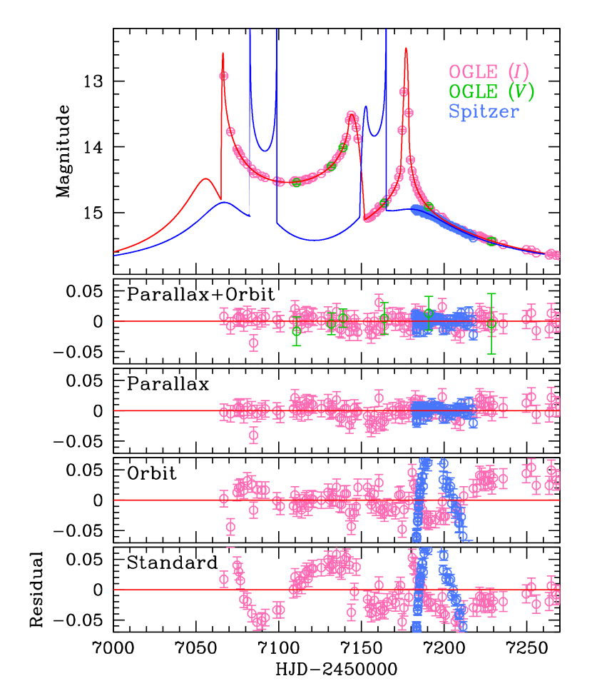
Figure 1.— Light curve of OGLE-2015-BLG-0196. The pink and light-blue dots in the upper panels show the data obtained from the ground-based observatory and Spitzer telescope, respectively. The lower four panels show the residuals from the 4 tested models. The solid curve superposed on the data points is the best-fit model (“parallax+orbit” model).

When the event was discovered, the light curve already deviated from the symmetric shape of a single-mass event. As the event progressed, the light curve exhibited a “U”-shape feature, which is a characteristic feature occurring when a source star passes the inner region of a binary-lens caustic. Since binary caustics form a closed curve, a caustic exit was expected and it actually happened on ${\rm HJD}^{\prime}={\rm HJD}-2450000\sim 7143$. From the preliminary modeling of the lensing light curve conducted after the caustic exit, it was anticipated that there would be another caustic-crossing feature at ${\rm HJD}^{\prime}\sim 7177$. The caustic feature occurred as predicted by the model. Subsequently, the light curve gradually returned to baseline.

In Figure 1, we present the light curve of OGLE-2015-BLG-0196, where the pink dots are the data obtained from the ground-based observations. The light curve is composed of 3 peaks that occurred at ${\rm HJD}^{\prime}\sim 7065$, 7143, and 7177. The first two peaks correspond to a caustic entrance and exit. The wide time gap of $\sim 78$ days between the caustic-crossing features indicates that the features resulted from the source crossing a large caustic. On the other hand, the third peak does not show a characteristic U-shape feature, suggesting the feature resulted from the source crossing over the cusp of the caustic. We note that the second and third caustic-crossing features were well resolved by ground-based observations. See the zoomed view of the resolved caustic-crossing features presented in Figure 2. The first caustic-crossing feature was not resolved because it occurred before the start of the 2015 bulge season. Another factor to be noted is the slow progress of the event. The event occurred before the beginning of the 2015 bulge season and proceeded throughout the whole bulge season.

The event was selected as a target for Spitzer observations because of the chance to measure the parallax effect between Spitzer and the Earth, which were separated by a projected separation of $D_{\perp}\sim 1.4\,$ au. It is particularly interesting to measure this effect for this binary since the caustic crossings are well resolved, meaning that the angular Einstein radius, and thereby the lens mass, could be determined from the measured $\theta_{\rm E}$ and $\pi_{\rm E}$ following Eq. (2). This binary was selected subjectively because it did not meet the objective binary criteria as described in Yee et al. (2015). The Spitzer observations of the event were conducted for $\sim 35$ days from ${\rm HJD}^{\prime}=7182.4$ to ${\rm HJD}^{\prime}=7217.5$. The observation cadence varies in the range $\sim 1/9$ – 1 day and the total number of data points is 65. The Spitzer data are presented in the upper panel of Figure 1 (blue dots).

Reduction of the ground-based data was done using the Difference Imaging Analysis pipeline (Udalski, 2003) of the OGLE survey. The Spitzer data were reduced using the algorithm specialized for Spitzer photometry in crowded fields (Calchi Novati et al., 2015b). For the individual data sets, we readjust error bars by

$$\sigma=k(\sigma_{0}^{2}+\sigma_{\rm min}^{2})^{1/2},$$ (3)

where $\sigma_{0}$ represents the error bar estimated from the automatized pipeline, $\sigma_{\rm min}$ is the factor used to make the error bars be consistent with the scatter of data points, and the other factor $k$ is used to make $\chi^{2}/{\rm dof}=1$. The adopted values of the scaling factor $k$ and the minimum error $\sigma_{\rm min}$ are $k=2.33$ and 0.40 and $\sigma_{\rm min}=0.005$ mag and 0.020 mag, for the OGLE and Spitzer data sets, respectively.

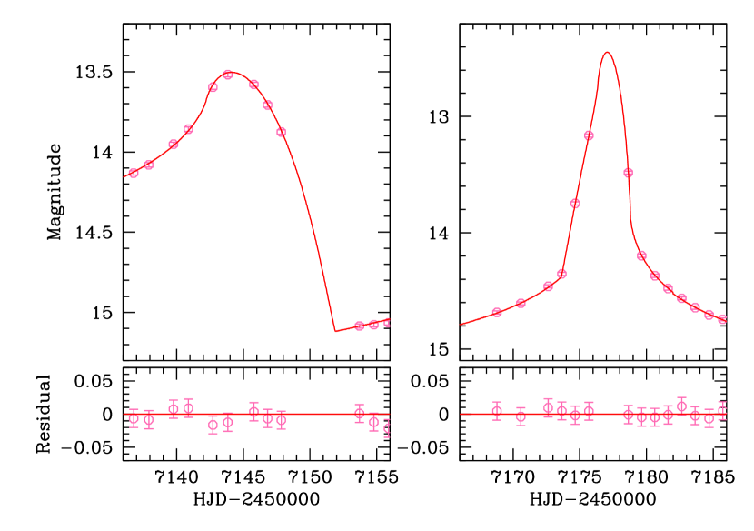
Figure 2.— Zoomed view of the light light curve around the second and third peaks at ${\rm HJD}^{\prime}={\rm HJD}-2450000\sim 7143$ and 7177.

3. Analysis

The number of parameters needed to model a binary event light curve in the simplest case of a rectilinear relative lens-source motion is 7 (principal parameters) plus 2 flux parameters for each data set. The principal parameters include the epoch of the closest lens-source approach, $t_{0}$, the lens-source separation at $t_{0}$, $u_{0}$, the Einstein time scale, $t_{\rm E}$, the separation $s$ and the mass ratio $q$ between the binary lens components, the angle between the source trajectory and the binary axis, $\alpha$, and the normalized source radius $\rho$. We note that lengths of the parameters $u_{0}$, $s$, $\rho$ are normalized to the angular Einstein radius $\theta_{\rm E}$ and the Einstein time scale $t_{\rm E}$ represents the time interval for the source to traverse $\theta_{\rm E}$. For the reference position of the lens, we use the barycenter of the binary lens. The flux parameters $F_{\rm S}$ and $F_{\rm B}$ represent the flux from the source and blend, respectively.

We start modeling of the event light curve with the 7 principal parameters (“standard model”). Modeling is performed in several steps. In the first step, a grid search is conducted for the parameters $s$, $q$, and $\alpha$ for which the lensing magnification is sensitive to small changes of the the parameters. The other parameters are optimized using a downhill approach, where we use the Markov Chain Monte Carlo (MCMC) method. In the second step, we locate local minima in the $\chi^{2}$ map of the parameters in order to check the existence of possible degenerate solutions which result in similar light curves despite the combinations of widely different parameters. In the last step, a global solution is identified from the comparison of the local solutions.

In computing lensing magnifications, we consider finite-source effects. Finite magnifications are computed by using both numerical and semi-analytic methods. In the region very close to caustics, we use the numerical ray-shooting method (Schneider & Weiss, 1986). In the region around the caustic, we use the semi-analytic hexadecapole approximation (Pejcha & Heyrovský, 2009; Gould, 2008). We also consider the limb-darkening effect of the source star. For this, the surface brightness variation is parameterized as $S_{\lambda}\propto 1-\Gamma_{\lambda}(1-3\cos\phi/2)$, where $\lambda$ denotes the filter used for observation and $\phi$ represents the angle between the normal to the source star’s surface and the line of sight toward the center of the source star. The adopted value of the limb-darkening coefficient is $\Gamma_{I}=0.62$, which is chosen from the catalog of Claret (2000) based on the stellar type of the source star. The source type is determined from the de-reddened color and brightness for which we discuss about the procedure of the determinations in section 4.

From the standard modeling, we find a unique solution that describes the three main caustic-crossing features of the ground-based light curve. From the solution, it is found that the lens is a binary object composed of similar-mass components and a projected separation slightly greater than $\theta_{\rm E}$. However, the solution leaves a significant residual from the model as presented in the bottom panel of Figure 1. The residual persists throughout the event, indicating that one should consider higher-order effects that cause long-lasting deviations. To be also noted is that the standard model provides a poor fit to the Spitzer data.

It is known that the orbital motion of a binary lens can cause long-term deviations in lensing light curves (Albrow et al., 2000; Shin et al., 2011; Park et al., 2013). Consideration of the orbital effect requires to include two additional parameters $ds/dt$ and $d\alpha/dt$, where $ds/dt$ denotes the rate of the binary separation change and $d\alpha/dt$ represents the change rate of the source trajectory angle. From the modeling considering the orbital effect (“orbit model”), we find that the observed data still leave a substantial residual from the model, indicating that the orbital effect is not the main cause of the deviation. In the third residual panel of Figure 1, we present the residual from the orbit model.

Another higher-order effect known to cause long-term deviations is the annual parallax effect. We check the possibility of the parallax effect by conducting another modeling considering the parallax effect (“parallax model”). This requires modeling with two additional parameters $\pi_{{\rm E},N}$ and $\pi_{{\rm E},E}$, which are the the components of $\mbox{\boldmath$\pi$}_{\rm E}$ projected onto the sky along the north and east equatorial coordinates, respectively.

Table 1Comparison of Models

Model		$\chi^{2}$
		OGLE+Spitzer	OGLE only
Standard		3123.7	1027.0
Orbit		2489.2	609.7
Parallax	($u_{0}<0$)	596.1	549.6
	($u_{0}>0$)	625.7	551.2
Parallax + Orbit	($u_{0}<0$)	571.7	524.0
	($u_{0}>0$)	572.8	525.1

Although parallax effects on the light curves obtained from ground-based and space-based observations manifest in different ways, the microlens parallax values measured through the different channels of the annual and the space-based microlens parallax observations should be the same. This implies that if the parallax effect detected in the light curve obtained from the ground-based observation is real, the effect should also be able to explain the light curve obtained from the Spitzer observation. Therefore, we conduct two sets of modeling where the first modeling is based on the ground-based data, while the second modeling is based on the combined data sets from the ground-based and from the Spitzer observations. From these modelings, we find that the parallax effect can explain both the deviations of the ground-based and the Spitzer data, as shown in the second residual panel of Figure 1. This indicates that the major cause of the deviation from the standard model is the parallax effect.

In the modeling considering parallax effects, we check the existence of degenerate solutions. It is a well-known fact that analyzing light curves of single-mass lensing events obtained from both space- and ground-based observations yields four sets of degenerate solutions (Gould, 1994), which are often denoted by $(+,+)$, $(-,-)$, $(+,-)$, and $(-,+)$, where the former and latter signs in each parenthesis represent the signs of the lens-source impact parameters as seen from Earth and from the satellite, respectively. In the case of binary-lensing, the four-fold parallax degeneracy collapses into a two-fold degeneracy for a general case of binary-lens events because the degeneracy between the pair of $(+,+)$ and $(+,-)$ [or $(-,-)$ and $(-,+)$] solutions are generally resolved due to the lack of lensing magnification symmetry compared to the single lens case although the remaining degeneracy, i.e. $(+,+)$ and $(-,-)$ solutions, may persist. However, Zhu et al. (2015) pointed that the four-fold degeneracy can persist in some special cases of the lens-source geometry. We, therefore, check the degeneracy by conducting a grid search in the $\pi_{{\rm E},N}$-$\pi_{{\rm E},E}$ parameter space. From this, we find that the light curve of OGLE-2015-BLG-0196 does not suffer from the degeneracy between $(\pm,\pm)$ and $(\pm,\mp)$ solutions and only the degeneracy between the $(+,+)$ and $(-,-)$ solutions persists. This degeneracy between the $(+,+)$ and $(-,-)$ solutions, which is referred to as the “ecliptic degeneracy” (Skowron et al., 2011), is known to exist for general binary-lens events. This degeneracy is caused because the two source trajectories with $u_{0}$ and $-u_{0}$ are in mirror symmetry with respect to the binary axis. For this reason, the degenerate $(+,+)$ and $(-,-)$ solutions are often denoted by $u_{0}>0$ and $u_{0}<0$ solutions, respectively. We note that the lensing parameters of the degenerate solutions caused by the ecliptic degeneracy are in the relation $(u_{0},\alpha,\pi_{{\rm E},N},d\alpha/dt)\leftrightarrow-(u_{0},\alpha,\pi_{{\rm E},N},d\alpha/dt)$ (Skowron et al., 2011).

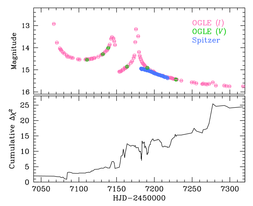
Figure 3.— Cumulative distribution of $\Delta\chi^{2}$ between the ”parallax only” model and the ”parallax + orbit” model. The lensing light curve in the upper panel is presented to show $\chi^{2}$ improvement with the progress of the event.

Table 2Best-fit Lensing Parameters

Parameter	OGLE+Spitzer		OGLE only
	$u_{0}<0$	$u_{0}>0$	$u_{0}<0$	$u_{0}>0$
$\chi^{2}$	571.7	572.8	524.0	525.1
$t_{0}$ (HJD-2450000)	7115.561 $\pm$ 0.916	7119.410 $\pm$ 0.954	7115.506 $\pm$ 0.489	7121.000 $\pm$ 0.968
$u_{0}$	-0.041 $\pm$ 0.004	0.044 $\pm$ 0.003	-0.037 $\pm$ 0.004	0.048 $\pm$ 0.004
$t_{\rm E}$ (days)	96.7 $\pm$ 0.6	92.9 $\pm$ 0.6	96.7 $\pm$ 0.6	92.9 $\pm$ 0.6
$s$	1.55 $\pm$ 0.01	1.61 $\pm$ 0.01	1.55 $\pm$ 0.01	1.63 $\pm$ 0.01
$q$	1.01 $\pm$ 0.02	1.10 $\pm$ 0.03	1.01 $\pm$ 0.02	1.15 $\pm$ 0.03
$\alpha$ (rad)	0.292 $\pm$ 0.013	-0.217 $\pm$ 0.011	0.304 $\pm$ 0.013	-0.248 $\pm$ 0.011
$\rho$ ($10^{-3}$)	8.31 $\pm$ 0.18	7.80 $\pm$ 0.13	8.57 $\pm$ 0.21	7.79 $\pm$ 0.19
$\pi_{{\rm E},N}$	0.171 $\pm$ 0.011	-0.116 $\pm$ 0.011	0.198 $\pm$ 0.016	-0.164 $\pm$ 0.018
$\pi_{{\rm E},E}$	0.105 $\pm$ 0.007	0.093 $\pm$ 0.006	0.100 $\pm$ 0.009	0.097 $\pm$ 0.014
$ds/dt$ (yr-1)	0.27 $\pm$ 0.06	0.01 $\pm$ 0.05	0.30 $\pm$ 0.06	-0.11 $\pm$ 0.08
$d\alpha/dt$ (rad yr-1)	-0.20 $\pm$ 0.05	-0.29 $\pm$ 0.03	-0.31 $\pm$ 0.06	-0.15 $\pm$ 0.06
$f_{{\rm S},I}$	7.27 $\pm$ 0.03	7.02 $\pm$ 0.05	7.27 $\pm$ 0.03	7.02 $\pm$ 0.05
$f_{{\rm B},I}$	0.11 $\pm$ 0.04	0.36 $\pm$ 0.05	0.11 $\pm$ 0.04	0.36 $\pm$ 0.05
$f_{{\rm S},V}$	0.16 $\pm$ 0.01	0.16 $\pm$ 0.01	0.16 $\pm$ 0.01	0.16 $\pm$ 0.01

Note. — The source and blending fluxes are normalized so that $f=1$ for an $I=18$ star.

Han et al. (2016b) pointed out that space-based microlens parallax observations can be useful not only for the microlens parallax measurement but also for the measurement of the orbital parameters. This is possible because the difference between the light curves seen from the ground and from a solar-orbit satellite produces a large parallax effect. At the same time, the features of the binary light curve as seen from the ground give precise timings for the caustic crossings. In the absence of space observations, these features give a measurement of the combination of parallax and orbital motion of the binary (which are partially degenerate (Batista et al., 2011; Skowron et al., 2011)). However, the microlens parallax is already mostly determined from the space-based parallax effect, so the information from the caustic crossing timing goes almost entirely into measuring the orbital motion. We, therefore, conduct an additional modeling, where both the orbital and the parallax effects are taken into account (“parallax + orbit” model). We find that the additional consideration of the orbital effect further improves the fit by $\Delta\chi^{2}=24.2$. Due to the small $\chi^{2}$ difference between the parallax only model and the parallax+orbit model, the improvement of the fit is is not immediately clear in the residuals. In Figure 3, we present the cumulative $\Delta\chi^{2}$ distribution to better show the improvement of the fit by the orbital effect. One finds that the fit improvement occurs throughout the event.

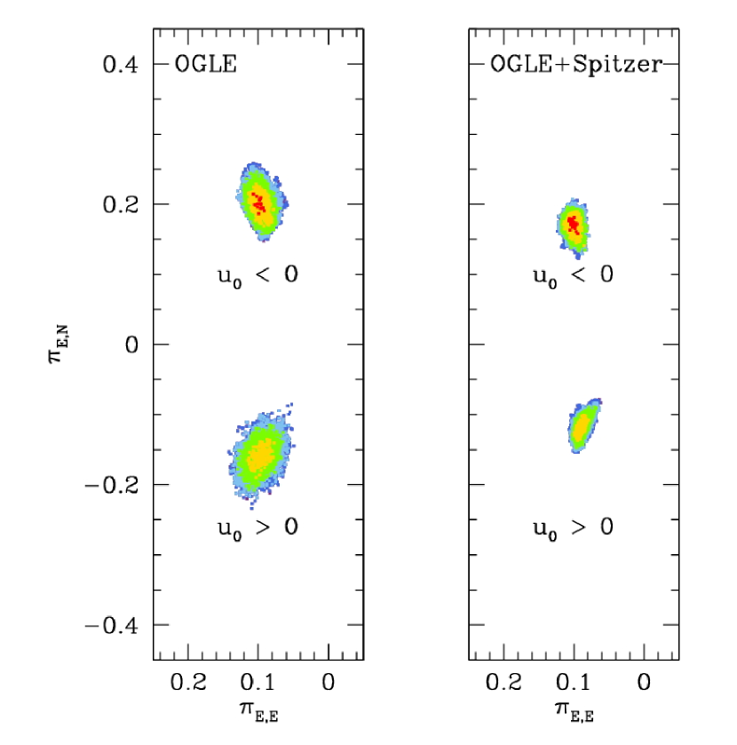
Figure 4.— Distribution of the microlens parallax parameters $\pi_{{\rm E},N}$ and $\pi_{{\rm E},E}$. The distributions in the left and right panels are obtained based on the ground-based OGLE data and the combined OGLE+Spitzer data, respectively. The color coding indicates points on the Markov Chain within 1$\sigma$ (red), 2$\sigma$ (yellow), 3$\sigma$ (green), 4$\sigma$ (cyan), and 5$\sigma$ (blue) of the best fit.

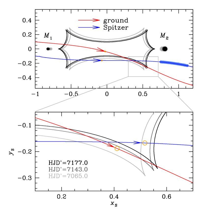
Figure 5.— Geometry of the lens system. The closed curve with six cusps is the caustic and the blue and red curves with arrows represent the source trajectories seen from the ground and from the Spitzer telescope, respectively. The caustic varies in time due to the orbital motion of the binary lens and we present 3 caustics corresponding to 3 different times marked in the lower panel. The lower panel shows the zoom of the region enclosed by a small box in the upper panel. The small orange circle at the tip of the arrow on the source trajectory represents the source size. The small filled dots marked by $M_{1}$ and $M_{2}$ are the binary-lens components. We note that $M_{1}$ is lighter in mass than $M_{2}$ because $M_{1}$ is defined as the lens component lying closer to the source trajectory. The points on the trajectory seen from the Spitzer telescope represent the source positions during the Spitzer observation. The coordinates are centered at the barycenter of the binary lens and all lengths are normalized to the angular Einstein radius corresponding to the total mass of the binary lens.

In Table 1, we present the $\chi^{2}$ values of the tested models in order to compare the goodness of the individual fits. For each model, we present both $\chi^{2}$ values determined based on the ground-based OGLE data and the combined OGLE+Spitzer data.

Figure 4 shows the distributions of the microlens parallax parameters $\pi_{{\rm E},N}$ and $\pi_{{\rm E},E}$ that are determined based on two different sets of data: one based on the ground-based OGLE data and the other based on the combined OGLE+Spitzer data. From the comparison of the distributions, one finds that the parallax parameters determined based on the two data sets match very well, indicating that the ground-based microlensing parallax is confirmed by the space-based observation. One also finds that the uncertainties of the parallax parameters based on the combined data is substantially smaller than the uncertainties based on only the ground-based data. This indicates that the Spitzer data add an important constraint on the parallax measurement despite the short coverage of the event.

In Table 2, we list the best-fit lensing parameters of the “parallax + orbit model” along with $\chi^{2}$ values. For comparison, we also present the parameters obtained based on the ground-based data. We find that the degeneracy between the $u_{0}<0$ and $u_{0}>0$ solution is very severe ($\Delta\chi^{2}=1.1$) and thus present both solutions. The estimated values of the normalized separation and the mass ratio between the binary lens components are $(s,q)=(1.55\pm 0.01,1.01\pm 0.02)$ for the $u_{0}<0$ solution and $(s,q)=(1.61\pm 0.01,1.10\pm 0.03)$ for the $u_{0}>0$ solution, indicating that the binary components have similar masses and the projected separation is $\sim 1.6$ times greater than the Einstein radius. We note that $q>1.0$ implies that the the lens component with the smaller separation from the source trajectory, $M_{1}$, is lighter in mass than the other lens component, $M_{2}$.

Figure 5 shows the lens system geometry (for the parallax + orbit model with $u_{0}<0$), where the trajectories of the source star with respect to the lens and the caustic are presented. We note that two source trajectories are presented: one seen from the ground (red curve) and the other seen from the Spitzer telescope (blue curve). Since the binary separation is not much different from the Einstein radius, the caustic is composed of a single big closed curve (resonant caustic) and it is elongated along the binary axis because $s>1$. We note that the caustic changes in time because the orbital motion of the binary lens causes the separation and the orientation of the binary lens to vary in time.

The ground-based source trajectory entered the upper left part of the caustic, diagonally passed the caustic, and then exited the caustic. Due to the concavity of the caustic curve, the source reentered the tip of the caustic, and then exited. It is found the two caustic-crossing spikes at ${\rm HJD}^{\prime}=7065$ and 7143 in the ground-based light curve were produced by the first set of the caustic entrance and exit, while the caustic feature at ${\rm HJD}^{\prime}=7177$ was produced by the second set of the caustic entrance and exit. The reason why the caustic-crossing feature at ${\rm HJD}^{\prime}=7177$ does not show a characteristic U-shape feature is that the width of the caustic tip is smaller than the source star and thereby the U-shape feature in the light curve is smeared out by finite-source effects. See the lower panel of Figure 5 where we present the zoomed view of the caustic tip.

The source seen from the Spitzer telescope took a different trajectory from the one seen from the ground. The source moved almost in parallel with the binary axis during which the caustic experienced two sets of caustic entrance and exit. The part of the light curve observed by the Spitzer telescope (marked by blue dots on the source trajectory in the upper panel of Figure 5) corresponds to the declining part after the second caustic exit.

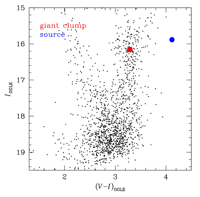
Figure 6.— Location of the source star in the color-magnitude diagram of stars in the neighboring region around the source star. The blue and red dots represent the source star and the centroid of giant clump, respectively.

Table 3Physical Parameters

Parameter	OGLE+Spitzer		OGLE only
	$u_{0}<0$	$u_{0}>0$	$u_{0}<0$	$u_{0}>0$
$M_{1}$ ($M_{\odot}$)	0.38 $\pm$ 0.04	0.50 $\pm$ 0.05	0.32 $\pm$ 0.04	0.39 $\pm$ 0.05
$M_{2}$ ($M_{\odot}$)	0.38 $\pm$ 0.04	0.55 $\pm$ 0.06	0.32 $\pm$ 0.04	0.44 $\pm$ 0.06
Distance to lens (kpc)	2.77 $\pm$ 0.23	3.30 $\pm$ 0.29	2.66 $\pm$ 0.23	2.78 $\pm$ 0.29
projected separation (AU)	5.30 $\pm$ 0.43	6.77 $\pm$ 0.59	4.83 $\pm$ 0.44	5.87 $\pm$ 0.59
Geocentric proper motion (mas yr-1)	4.66 $\pm$ 0.37	5.00 $\pm$ 0.40	4.43 $\pm$ 0.38	5.08 $\pm$ 0.41
KE/PE	0.17	0.32	0.30	0.09

4. Lens Parameters

For the unique determination of the lens mass and distance, one additionally needs the angular Einstein radius in addition to the microlens parallax. The angular Einstein radius is determined from the normalized source radius $\rho$ and the angular source radius $\theta_{*}$ by

$$\theta_{\rm E}={\theta_{*}\over\rho}.$$ (4)

The value of $\rho$ is determined by analyzing the resolved caustic crossings that are affected by finite-source effects.

We estimate the angular source radius from the stellar type determined based on the de-reddened color $(V-I)_{0}$ and brightness $I_{0}$. For this, we first measure the instrumental $I$-band magnitude from the flux parameters $F_{{\rm S},I}$ and $F_{{\rm B},I}$ and the instrumental color $V-I$ from the source flux $F_{{\rm S},I}$ and $F_{{\rm S},V}$ determined from the modeling based on the $I$- and $V$-band OGLE data. In Figure 6, we mark the source position $(V-I,I)=(4.16,15.85)$ in the instrumental color-magnitude diagram of the field around the source star of OGLE-2015-BLG-0196. We calibrate the color and brightness of the source star using the giant clump (GC) centroid in the color-magnitude diagram (Yoo et al., 2004). The centroid of GC, marked by a red dot in Figure 6, can be used for calibration because (1) the de-reddened color $(V-I)_{0,{\rm GC}}=1.06$ (Bensby et al., 2011) and the magnitude $I_{0,{\rm GC}}=14.6$ (Nataf et al., 2013) are known and (2) the source and GC stars are located in the bulge and thus experience a similar amount of extinction. The source distance is estimated using the relation $D_{\rm S}=D_{\rm GC}/(\cos l+\sin l/\tan\phi)$ (Nataf et al., 2013), where $D_{\rm GC}=8160$ pc is the galactocentric distance and $\phi=40^{\circ}$ is the angle between the bulge’s major axis and the line of sight. From the difference in color and magnitude between the source star and the GC centroid, we estimate $(V-I,I)_{0}=(1.87,14.3)$, indicating that the source is a very red M-type giant. We covert $V-I$ into $V-K$ using the relation provided by Bessell & Brett (1988), and then derive $\theta_{*}$ from the relation between the $V-K$ and surface brightness (Kervella et al., 2004). It is estimated that the source star has an angular radius of

$$\theta_{*}=10.25\pm 0.83\ \mu{\rm as}.$$ (5)

From the measured $\theta_{*}$ and $\rho$, it is estimated that the angular Einstein radius of the lens system is

$$\theta_{\rm E}=1.23\pm 0.10\ {\rm mas}\ \ (1.27\pm 0.10\ {\rm mas}),$$ (6)

where the values in and out of the parenthesis are the values for the $u_{0}<0$ and $u_{0}>0$ solution, respectively.

By measuring both $\theta_{\rm E}$ and $\pi_{\rm E}$, the masses of the lens components are determined as

$$M_{1}=0.38\pm 0.04\ M_{\odot}\ (0.50\pm 0.05\ M_{\odot})$$ (7)

for the lens component located closer to the source trajectory and

$$M_{2}=0.38\pm 0.04\ M_{\odot}\ (0.55\pm 0.06\ M_{\odot})$$ (8)

for the other lens component. The distance to the lens is

$$D_{\rm L}=2.77\pm 0.23\ {\rm kpc}\ (3.30\pm 0.29\ {\rm kpc}).$$ (9)

The estimated mass and distance indicate that the binary lens is composed of roughly equal-mass M dwarf stars and located in the disk of the Galaxy. The binary components are separated in projection by

$$r_{\perp}=5.30\pm 0.43\ {\rm au}\ (6.77\pm 0.59\ {\rm au}).$$ (10)

In Table 3, we summarize the physical lens parameters. We note that the notation “KE/PE” represents the ratio of the transverse kinetic to potential energy that is computed by

$$\left({{\rm KE}\over{\rm PE}}\right)_{\perp}={(r_{\perp}/{\rm au})^{3}\over 8\pi^{2}(M/M_{\odot})}\left[\left({1\over s}{ds\over dt}\right)^{2}+\left({d\alpha\over dt}\right)^{2}\right],$$ (11)

where $M=M_{1}+M_{2}$. The ratio should be less than the three-dimensional kinetic to potential energy ratio, KE/PE, and should be less than unity for the system to be bound, i.e. $({\rm KE}/{\rm PE})_{\perp}\leq{\rm KE}/{\rm PE}<1$. The determined $({\rm KE}/{\rm PE})_{\perp}$ satisfies this requirement.

5. Conclusion

We analyzed the binary-lensing event OGLE-2015-BLG-0196 that was observed both from the ground and from the Spitzer Space Telescope. The light curve obtained from ground-based observations exhibited significant deviations from the lensing model based on the rectilinear relative lens-source motion motion and analysis of the deviation allowed us to measure the microlens parallax. The measured microlens parallax was confirmed by the data obtained from space-based observations up to the two-fold degeneracy caused by the well-known ecliptic degeneracy. This event is the first case where the ground-based microlens parallax was firmly confirmed with space-based observations. By additionally measuring the angular Einstein radius from the analysis of caustic crossings of the light curve, we determined the mass and distance to the lens. It was found that the lens is a binary composed of roughly equal-mass M dwarf stars located in the Galactic disk.

References

- Albrow et al. (2000) Albrow, M. D., Beaulieu, J.-P., Caldwell, J. A R., et al. 2000, ApJ, 534, 894
- Batista et al. (2011) Batista, V., Gould, A., Dieters, S., et al. 2011, A&A, 529, 102
- Bensby et al. (2011) Bensby, T., Adén, D., Melńdez, J., et al. 2011, A&A, 533, A134
- Bessell & Brett (1988) Bessell, M. S., & Brett, J. M. 1988, PASP, 100, 1134
- Bozza et al. (2016) Bozza, V., Shvartzvald, Y., Udalski, A., et al. 2016, ApJ, 820, 79
- Calchi Novati et al. (2015a) Calchi Novati, S., Gould, A., Udalski, A., et al. 2015a, ApJ, 804, 20
- Calchi Novati et al. (2015b) Calchi Novati, S., Gould, A., Yee, J. C., et al. 2015b, ApJ, 814, 92
- Claret (2000) Claret, A. 2000, A&A, 363, 1081
- Dong et al. (2007) Dong, S., Udalski, A., Gould, A., et al. 2007, ApJ, 664, 862
- Gould (1992) Gould, A. 1992, ApJ, 392, 442
- Gould (1994) Gould, A. 1994, ApJ, 421, L75
- Gould (2000) Gould, A. 2000, ApJ, 542, 785
- Gould (2008) Gould, A. 2008, ApJ, 681, 1593
- Han et al. (2016a) Han, C., Udalski, A., Gould, A., et al. 2016a, ApJ, 828, 53
- Han et al. (2016b) Han, C., Udalski, A., Lee, C.-U., et al. 2016b, ApJ, 827, 11
- Henderson et al. (2016) Henderson, C. B., Poleski, R., Penny, M., et al. 2016, ApJ, submitted
- Kervella et al. (2004) Kervella, P., Bersier, D., Mourard, D., et al. 2004, A&A, 428, 587
- Muraki et al. (2011) Muraki, Y., Han, C., Bennett, D. P., et al. 2011, ApJ, 741, 22
- Nataf et al. (2013) Nataf, D. H., Gould, A., Fouqué, P., et al. 2013, ApJ, 769, 88
- Park et al. (2013) Park, H., Udalski, A., Han, C., et al. 2013, ApJ, 778, 134
- Pejcha & Heyrovský (2009) Pejcha, O., & Heyrovský, D. 2009, ApJ, 690, 1772
- Refsdal (1966) Refsdal, S. 1966, MNRAS, 134, 315
- Schneider & Weiss (1986) Schneider, P., & Weiss, A. 1986, A&A, 164, 237
- Shin et al. (2011) Shin, I.-G., Udalski, A., Han, C., et al. 2011, ApJ, 735, 85S
- Shvartzvald et al. (2016) Shvartzvald, Y., Li, Z., Udalski, A., et al. 2016, arXiv:1606.02292
- Shvartzvald et al. (2015) Shvartzvald, Y., Udalski, A., Gould, A., et al. 2015, ApJ, 814, 111
- Skowron et al. (2011) Skowron, J., Udalski, A., Gould, A., et al. 2011, ApJ, 738, 87
- Street et al. (2016) Street, R. A. Udalski, A., Calchi Novati, A., et al. 2016, ApJ, 819, 93
- Udalski (2003) Udalski, A. 2003, AcA, 53, 291
- Udalski et al. (2015) Udalski, A., Szymański, M. K., & Szymański, G. 2015, AcA, 65, 1
- Udalski et al. (2015) Udalski, A., Yee, J. C., Gould, A., et al. 2015, ApJ, 799, 237
- Yee et al. (2015) Yee, J. C., Udalski, A., Calchi Novati, S., et al. 2015, ApJ, 802, 7
- Yoo et al. (2004) Yoo, J., DePoy, D. L., Gal-Yam, A., et al. 2004, ApJ, 603, 139
- Zhu et al. (2016) Zhu, W., Calchi Novati, S., Gould, A., et al. 2016, ApJ, 825, 60
- Zhu et al. (2015) Zhu, W., Udalski, A., Gould, A., et al. 2015, ApJ, 805, 8