Inferring low-dimensional microstructure representations using convolutional neural networks

Abstract

We apply recent advances in machine learning and computer vision to a central problem in materials informatics: The statistical representation of microstructural images. We use activations in a pre-trained convolutional neural network to provide a high-dimensional characterization of a set of synthetic microstructural images. Next, we use manifold learning to obtain a low-dimensional embedding of this statistical characterization. We show that the low-dimensional embedding extracts the parameters used to generate the images. According to a variety of metrics, the convolutional neural network method yields dramatically better embeddings than the analogous method derived from two-point correlations alone.

I Introduction

A central problem in materials design is the analysis, characterization, and control of materials microstructure. Microstructure is generated by non-equilibrium processes during the formation of the material and plays a large role in the bulk material’s properties Kumar et al. (2006); Ostoja-Starzewski (2007); Wang and Pan (2008); Fullwood et al. (2010); Torquato (2010). In recent years, machine learning and informatics based approaches to materials design have generated much interest Rajan (2013); Kalidindi (2015); Lookman et al. (2016); Voyles (2017); Xue et al. (2016). Effective statistical representation of microstructure has emerged as an outstanding challenge Kalidindi et al. (2011); Liu et al. (2013); Niezgoda et al. (2013).

Standard approaches begin with an $n$-point expansion, and typically truncate at the pair correlation level Jiao et al. (2007); Fullwood et al. (2008); Jiao et al. (2009); Chen et al. (2014). Pair correlations can capture information such as the scale of domains in a system, but miss higher order complexities such as the detailed shape of domains or relative orientation of nearby domains Jiao et al. (2010a, b); Gommes et al. (2012a, b). Three-point correlations (and successors) quickly become computationally infeasible, as the number of $n$-point correlations scales exponentially with $n$. Furthermore, they are not tailored to capture the statistical information of interest. Much current work involves deploying a set of modified two-point correlations to better capture certain microstructural features Jiao et al. (2009); Niezgoda et al. (2008); Zachary and Torquato (2011); Gerke et al. (2014); Xu et al. (2014).

Independently, researchers in machine learning for computer vision have been developing powerful techniques to analyze image content Lecun et al. (1998); Krizhevsky et al. (2012); Simonyan and Zisserman (2014); Szegedy et al. (2015); He et al. (2016). Deep Convolutional Neural Networks (CNNs) have emerged as a particularly powerful tool for image analysis LeCun et al. (2015). Of particular interest to materials microstructure analysis is literature regarding texture reconstruction and modeling Hao et al. (2012); Kivinen and Williams (2012); Luo et al. (2013); Gao and Roth (2014); Theis and Bethge (2015); in this context a texture is an image with roughly translation invariant statistics. Indeed, Gatys et al. have recently demonstrated that correlations between CNN activations capture the statistics of textures exceptionally well Gatys et al. (2015, 2016).

Here, we apply the Gatys et al. CNN texture vector representation of image statistics to the problem of characterizing materials micrographs. The texture vector is a statistical representation of an image derived from the processing of a pre-trained CNN; we use the Visual Geometry Group’s VGG-19 network Simonyan and Zisserman (2014), which has been trained to classify 1.2 million natural images Russakovsky et al. (2015). We demonstrate that the texture vectors generated using the VGG-19 network can capture complex statistical correlations visible in microstructure images in Fig. 1. Specifically, we use the CNN texture vector to characterize an original microstructural image, and then generate a new, random image constrained to the same statistics. It is remarkable that using only a single original image, the algorithm generates texture images nearly indistinguishable to the eye. In the case of materials micrographs, where data can be expensive to collect, the ability for a method perform well on small datasets is crucial. Our approach can be considered one of transfer learning, i.e., the application of a model trained on one problem to achieve results on a different, but related problem. The fidelity in Fig. 1 motivates us to pursue the CNN texture vector as a tool for mapping relationships between materials processing, microstructure, and properties.

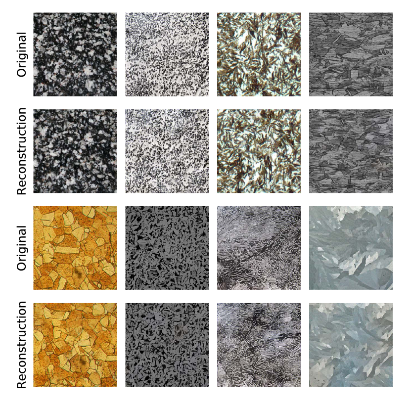
Figure 1: (Color online) Texture synthesis of materials microstructures using the CNN algorithm from Gatys et al. (2015). The CNN synthesizes each “Reconstruction” image from a single “Original” image. (Image attributions listed in Appendix A.)

As a step towards microstructure analysis, we demonstrate and quantify the ability of the CNN texture vector to extract hidden information from a collection of synthetic texture images. Images in our datasets are generated under different “processing” conditions, i.e. a few generating parameters. The goal is to extract a compact statistical representation of the dataset that captures the relevant statistics associated with the hidden generating parameters—that is, to back out the processing parameters of micrographs directly from the images alone. Our use of synthetic data, with a tightly controlled ground truth, provides us quantitative measures of error in the unsupervised learning process.

Despite being very high-dimensional, the CNN texture vector offers a good notion of abstract distance between texture images: The closer the generating parameters, the smaller the distance between texture vectors. We use manifold learning to embed each image as a point in a low-dimensional space such that, ideally, the embedded distances match the texture vector distances. The structure of the embedded points then reveals information about the set of images. For our synthetic dataset, we show a simple relationship between the embedded coordinates and the generating parameters. More broadly, dimensionality reduction techniques may serve as the basis for characterization of materials properties that are controlled by complex materials microstructures. A recent example is the work of Ref. DeCost et al., 2017, which uses a method similar to ours to map the space of ultrahigh carbon steel microstructures.

Our approach applies unsupervised learning, a pattern-discovery framework to seek new aspects of microstructure without using labeled data. This approach is applicable to problems where the ground truth is unknown, e.g., the forensic analysis of microstructures. Several recent applications of machine learning to microstructure have used supervised learning algorithms Sundararaghavan and Zabaras (2005); DeCost and Holm (2015); Kalinin et al. (2015); Liu et al. (2015); Bostanabad et al. (2016); Chowdhury et al. (2016); Orme et al. (2016) such as support vector machines and classification trees, which make inferences based on labeled data. Like our work, Ref. Chowdhury et al., 2016 uses image features extracted from CNNs to aid microstructure analysis.

The remainder of the paper is organized as follows: Section II gives background on recent CNN architectures for image recognition, and specifics of the VGG network. Section III details our algorithms for statistical microstructure analysis and Sec. IV evaluates their accuracy on test datasets. Section V provides discussion and interpretation of our results, and we conclude in Sec. VI.

II Review of Convolutional Neural Networks

CNNs have emerged in recent years as state-of-the-art systems for computer vision tasks Lecun et al. (1998); Krizhevsky et al. (2012); Simonyan and Zisserman (2014); Szegedy et al. (2015). They form a modern basis for image recognition and object detection tasks, and in some cases now outperform humans He et al. (2015, 2016).

The basic computational structure is that of a many-layered (i.e., deep) artificial neural network. For a brief overview, see Ref. LeCun et al., 2015; for a comprehensive text, see Ref. Goodfellow et al., 2016. There are a great variety of deep neural network architectures; here we first focus on the core components. Each layer in the network contains many computational units (neurons). Each neuron takes a set of inputs from the previous layer and computes a single output (the activation) to be used as an input in the next layer. Each neuron’s activation is constructed as follows: First, the set of inputs is linearly combined into a scalar using a set of weights and shifted using a bias. To this sum, the neuron applies a simple nonlinear map, the activation function, to generate its activation.

In the learning phase, the network is trained by iteratively tuning the weights and biases so that the network better performs a task. Performance of the network is quantified by a scalar objective function. Commonly, a network is trained by supervised learning, in which the network learns a mapping from inputs to outputs using a database of training examples. In this case, the objective function is a measure of error in the network output summed over all examples of the training set. The objective function is often differentiable and optimized via stochastic gradient descent.

A CNN is a specific type of artificial neural network which is useful for processing data on a spatial and/or temporal grid. The convolutional layers in CNNs impose strong restrictions on the structure of weights: Each layer consists of a bank of trainable filters (sometimes called kernels) that are convolved with activations from the previous layer. The convolution outputs are called activation maps. This technique of constraining and reusing weights is called weight tying. Note that the convolutional structure preserves spatial locality: The activation maps at each convolutional layer are interpretable as images. As in a plain artificial neural network, each pixel in the output image is passed through a nonlinear activation function. CNNs also commonly include pooling layers that effectively coarse-grain the image plane. These layers operate by taking a statistic over a small region of the image plane, such as the maximum of a feature’s activations in a $2\times 2$ pixel region. Importantly, the convolutional and pooling layers process the input image in a (nearly) translation equivariant way. This directly encoded translational symmetry is designed to match that of natural images, which as a distribution exhibit repeated patterns centered at a variety of locations. By alternating between sets of convolution and pooling layers, CNNs are able to develop sensitivity to very complex correlations over large length scales, which underlies their strong performance on image recognition tasks.

As in Gatys et al. Gatys et al. (2015, 2016), our work begins with a normalized version of the Visual Geometry Group’s VGG-19 network Simonyan and Zisserman (2014) already trained to classify natural images. The VGG-19 network placed first in localization and second in classification in the ILSVRC 2014 ImageNet Challenge Russakovsky et al. (2015). The VGG network is known for its simple architecture and competitive performance. The convolutional kernels each have a $3\times 3$ pixel spatial extent. The nonlinear activation function applied after each convolution is a rectifier (ReLU), $f(x)=\max(0,x)$. The convolutional layers are applied in a series of blocks, and between the blocks, pooling layers are applied (in the original network, Max pooling, but here as in Refs. Gatys et al., 2015 and Gatys et al., 2016 we use Mean pooling). Blocks one and two contain two convolutions each, and blocks three, four, and five contain four convolutions each. The final stage of the network adds three fully connected layers—these do not directly encode spatial information, and so are not used for translation invariant characterization of images. We used the optimizing compiler Theano Theano Development Team (2016) and the neural network library Lasagne Dieleman et al. (2015) to implement the CNN methods used in this paper.

III Methods

III.1 CNN texture vector representation of image statistics

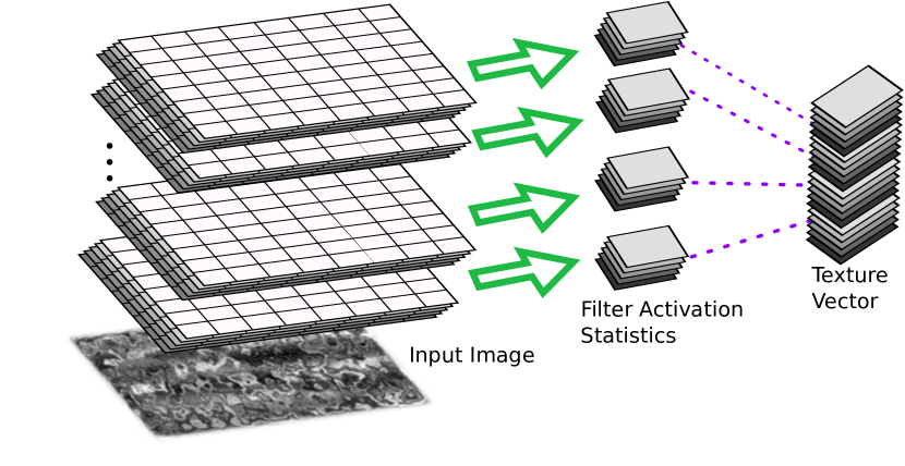
Figure 2: A schematic view of the creation of a texture vector representation of an image using a CNN. The input image is processed upward through multiple CNN layers. Activations at each layer produce a stack of filtered images. Correlations between filtered images, averaged over the image plane, are collected. These statistics are then concatenated (with optional weighting) to form a texture vector. The activations at higher layers capture texture information over larger spatial scales.

Gatys et al. Gatys et al. (2015, 2016) have developed a robust algorithm for statistical analysis of texture images relevant to materials microstructure, which we demonstrated in Fig. 1. Given an input texture image, the Gatys procedure extracts a texture vector from activations in the convolutional layers. This calculation is summarized in Fig. 2. Activations in the CNN are denoted by $F_{ij}^{l}$, where $l$ is the layer index, $i$ is the feature index, and $j$ is the pixel index. At each layer, the Gram matrix captures correlations between feature $i$ and feature $k$,

$$G^{l}_{ik}=\sum_{j}F_{ij}^{l}F_{kj}^{l}.$$ (1)

The summation over pixel index $j$ encodes invariance to translations in the image plane (up to boundary effects). Compared to the mean feature activations $\sum_{j}F_{ij}^{l}$ alone, the Gram matrix offers much richer statistical information Gatys et al. (2015). In the following we suppress feature indices $i$ and $k$ and view the Gram matrix, $G^{l}_{ik}\rightarrow G^{l}$, as a summary of activation statistics on layer $l$. For the purposes of texture synthesis, Gatys et al. introduce a scalar, positive-definite loss between two images $x_{i}$ and $x_{j}$ (let us note explicitly that $i$ and $j$ now index images) with Gram matrices $G^{l}(x_{i})$ and $G^{l}(x_{j})$:

$$L^{l}(x_{i},x_{j})=\frac{1}{A_{l}}||G^{l}(x_{i})-G^{l}(x_{j})||^{2},$$ (2)

with $||\cdot||$ the Euclidean norm. $A_{l}=4N_{l}^{2}M_{l}^{2}$ is a normalization factor for the loss on layer $l$ with $N_{l}$ features and $M_{l}$ pixels. The total loss is the weighted sum of layer-wise losses,

$$L(x_{i},x_{j})=\sum_{l}w_{i}L^{l}(x_{i},x_{j}).$$ (3)

In this work we use the VGG network Simonyan and Zisserman (2014), normalized as in Gatys et al. (2015, 2016), and apply equal weight ($w_{l}=1$) to each of the following layers: “conv1_1”, “conv2_1”, “conv3_1”, “conv4_1”, and “conv5_1”. It is convenient to define rescaled Gram matrices, $\hat{G}^{l}=(w_{l}/A_{l})G^{l}$. Their concatenation $\hat{G}=(\hat{G}^{1},\hat{G}^{2},\cdots)$ is the scaled texture vector. The layers we use have feature sizes of $[N_{1},N_{2},\ldots]=[64,128,256,512,512]$, resulting in a total texture vector length of $\sum_{l}N_{l}^{2}\approx 5\cdot 10^{5}$ elements. From the texture vector of two images, we may form a distance between images

$$d_{ij}^{2}=||\hat{G}(x_{i})-\hat{G}(x_{j})||^{2}=L(x_{i},x_{j}).$$ (4)

That is, $\hat{G}$ as a function endows two images $x_{i}$ and $x_{j}$ with a Euclidean distance $d_{ij}$ based on their texture representations within the CNN. We will show that this distance is a useful input to machine learning algorithms, and in particular, manifold learning (see Sec. III.3).

III.2 Power spectrum statistics

To benchmark the CNN texture vector representation, we compare it against the power spectrum (PS) associated with two-point correlations in the image. This approach is commonly employed for statistical characterization of microstructure. Our test dataset contains single-component (grayscale) images $x_{i}$, each represented as a scalar field $\phi_{i}(\mathbf{r})$. Assuming translation invariance, the two-point correlation function of $\phi(\mathbf{r})$ is

$$P_{2}(\Delta\mathbf{r})=\int\phi(\mathbf{r}^{\prime})\phi(\mathbf{r}^{\prime}+\Delta\mathbf{r})~{}\mathrm{d}\mathbf{r}^{\prime}.$$ (5)

If ensemble averaged, the full set of $n$-point correlation functions would capture all information about the statistical distribution of images.

The PS (also known as the structure factor) $S(\mathbf{q})$ is the Fourier transform of $P_{2}$, which can be expressed as

$$S(\mathbf{q})=\tilde{\phi}(\mathbf{q})\tilde{\phi}(-\mathbf{q})=|\tilde{\phi}(\mathbf{q})|^{2},$$ (6)

where $\tilde{\phi}(\mathbf{q})$ is the Fourier transform of $\phi(\mathbf{r})$. For this analysis, we compute the PS after rescaling $\phi(\mathbf{r})$ to the range $[-1,1]$.

To develop low-dimensional representations of microstructures, we require a distance between microstructures. Given two images $x_{i}$ and $x_{j}$ and their respective power spectra $S_{i}(\mathbf{q})$ and $S_{j}(\mathbf{q})$, we obtain a new distance $d_{ij}$ between the images,

$$d_{ij}^{2}=\int\left[S_{i}(\mathbf{q})-S_{j}(\mathbf{q})\right]^{2}\mathrm{d}\mathbf{q},$$ (7)

which should contrasted with the CNN distance in Eq. (4).

III.3 Manifold Learning with Multidimensional Scaling

To assess the quality of the texture vectors for characterizing images we perform manifold learning. The goal of manifold learning is to find a low-dimensional representation of the data that faithfully captures distance information [here, from Eq. (4) or (7)]. Multidimensional Scaling Kruskal (1964); Borg and Groenen (2005); Franklin (2008) (MDS) implements this principle as follows: Given a dataset $\{x_{i}\}$, a distance function $d_{ij}=d(x_{i},x_{j})$ between datapoints, and an embedding dimension $D^{\ast}$, the goal is to find embeddings $x_{i}\mapsto\hat{x}_{i}\in\mathbb{R}^{D^{\ast}}$ such that the embedded Euclidean distance $\hat{d}_{ij}=||\hat{x}_{i}-\hat{x}_{j}||$ best matches $d_{ij}$, i.e. minimizes a stress function $\sigma$. Here, we use Kruskal’s stress Kruskal (1964),

$$\sigma=\sqrt{\frac{\sum(d_{ij}-\hat{d}_{ij})^{2}}{\sum d_{ij}^{2}}}$$ (8)

We will consider embedding dimensions $D^{\ast}\lesssim 10$, which is very small compared to the dimension of the full CNN texture vector, roughly $2.5\times 10^{5}$ (Sec. III.1).

Note that MDS seeks $\hat{d}_{ij}$ that globally matches distances $d_{ij}$, and thus captures information about all image pairs. Other schemes, such as Local Linear Embedding Roweis and Saul (2000) or Isomap Tenenbaum et al. (2000), instead work with a local sparsification of the distance matrix $d_{ij}$. In this work, we select MDS because of its direct interpretibility and conceptual simplicity. MDS requires only one hyperparameter, the embedding dimension $D^{\ast}$. We use the scikit-learn Pedregosa et al. (2011) implementation of MDS, which applies an iterative majorization algorithm De Leeuw (1977) to optimize the embedding stress $\sigma$, Eq. (8).

IV Tasks

IV.1 Image generation process

We argue that although the space of materials microstructure is very rich, it will admit an effective low-dimensional representation. For example, a description of the materials processing (e.g. composition, thermodynamic variables and their rates of change) should be more compact than a direct description of the resulting microstructure. A statistical analysis of microstructure is valuable in that it may lead to further dimensionality reduction; multiple different processing paths may lead to the same microstructure. In this work, we study a database of synthetic 2-D microstructure images generated from a stochastic process with a few tunable generating variables. We use Perlin noise Perlin (1985) to generate marble-like stochastic images. The method procedurally calculates a smooth multi-scale noise function $\mathbf{h}(\mathbf{r})$ that generates distorted spatial points $\mathbf{u}_{A}=\mathbf{r}\,+\,A\,\mathbf{h}(\mathbf{r})$ with noise amplitude $A$. Then each texture image $x_{i}$ is realized as a 2-D scalar field

$$\phi_{i}(\mathbf{r})=\cos[2\pi k_{i}\,\mathbf{u}_{A_{i}}\cdot\mathbf{\mathbf{\hat{n}}}_{\theta_{i}}],$$ (9)

where $\mathbf{\hat{n}}_{\theta}$ is a unit vector with angle $\theta$. That is, each image $x_{i}$ consists of sinusoidal oscillation parameterized by angle ($\theta_{i}$), scale ($k_{i}$), and noise amplitude ($A_{i}$) parameters. This three-dimensional parameter space is shown in Fig. 3.

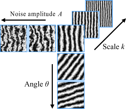
Figure 3: The space of synthetic textures, generated by tunable parameters $A$, $k$, and $\theta$.

Figure 4 illustrates the multi-scale nature of the set $\{x_{i}\}$ of stochastic texture images. At small noise values, the power spectrum is peaked on two Fourier modes. With increasing noise amplitudes, the peaks of the power spectrum broaden.

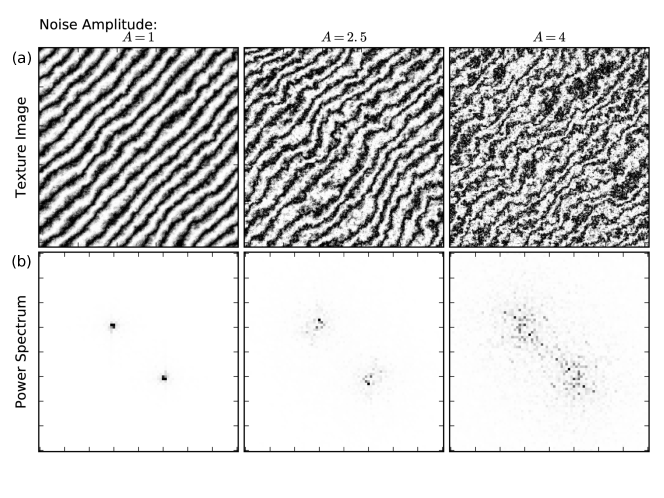
Figure 4: Row (a): Synthetic microstructures with scale parameter $k=15$ and varying noise amplitudes $A$. Row (b): Associated power spectrum, zoomed to relevant region of Fourier space. To aid visualization, the intensities are scaled by factors of approximately 1, 3, and 100, such that their maxima appear equally dark.

IV.2 Angle reconstruction task

Our first task is to reconstruct a 1-D manifold of images of fixed noise amplitude and scale parameter, but varying angle. For each trial, the scale parameter was fixed to $k=15$, corresponding to a modulation wavelength of $1/15$ in units of the linear system size. The angles $\theta_{i}$ take values $(i/N)\pi$ for $i\in\{0,1,\dots N-1\}$. Note that $0\leq\theta<\pi$ without loss of generality because $\mathbf{\hat{n}}_{\theta}=-\mathbf{\hat{n}}_{\theta+\pi}$ and thus $\theta$ and $\theta+\pi$ are equivalent for our textures, Eq. (9). In this subsection we explore datasets with varying dataset sizes $N$ and noise amplitudes $A$. We compute distances between the images via the CNN (Sec. III.1) and PS (Sec. III.2) methods, then use MDS (Sec. III.3) to map the images into a $D^{\ast}=2$ embedding space.

We quantify reconstruction quality as follows: First, we find the center of mass of all points in the embedded space, and use this as the origin. Second, we calculate angles $\varphi_{i}$ about the origin, which are unique up to a single additive constant $c$. Finally, we seek a correspondence between the generating angles $\theta_{i}$ and the learned values $\varphi_{i}/2$. The factor of $1/2$ is necessary because $\theta_{i}$ ranges from $0$ to $\pi$ whereas $\varphi_{i}$ ranges from $0$ to $2\pi$. We select the constant $c$ to minimize the root-mean-square error,

$$\mathrm{RMSE}=\sqrt{\frac{1}{N}\sum_{i}[\theta_{i}-(\varphi_{i}+c)/2]^{2}}$$ (10)

Once $c$ is optimized, we use the RMSE to measure the reconstruction quality.

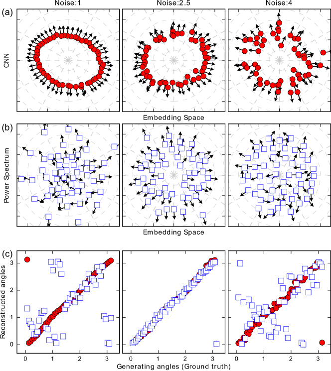
Figure 5: (Color online) Angle reconstructions. Each dataset contains $N=50$ images with varying angles $\theta_{i}$, fixed scale $k=15$, and fixed noise amplitude $A\in\{1,2.5,4\}$. Red circles correspond to the CNN method (Sec. III.1) and blue squares correspond to the PS method (Sec. III.2). Row (a): MDS embedded points $\hat{x}_{i}$ using the CNN method. Arrows represent $2\theta_{i}$ where $\theta_{i}$ is the angle used to generate image angles. Row (b): MDS embedded points $\hat{x}_{i}$ using the PS method. Row (c): Comparison of $\theta_{i}$ with corresponding angle $(\varphi_{i}+c)/2$ reconstructed from the embedding space. The CNN method yields excellent agreement, and clearly outperforms the PS method.

Figure 5 shows embedded manifolds and corresponding angle reconstructions using dataset size $N=50$ and noise amplitudes $A\in\{1,2.5,4\}$. For low noise amplitudes $A=1$, the CNN distances produce a ring structure which reflects the generating angles (and associated periodicity) quite well, whereas the PS method fails. For intermediate $A=2.5$, both CNN and PS distances generate good angle reconstructions, but there is much less scatter in the CNN embeddings. For large $A=4$, the CNN continues to give good angle reconstructions despite scatter in the embedded points, whereas the PS method again fails. Note that, by construction, the PS method is rotationally symmetric, whereas the CNN method encodes rotational symmetry only approximately. Consequently, the CNN embeddings are somewhat elliptical.

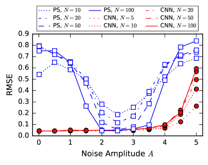
Figure 6: (Color online) The angle reconstruction error, Eq. (10), as a function of noise amplitude $A$, with scale $k=15$. Each dataset consists of $N$ images with varying angle $\theta_{i}$. The CNN method performs well across a wide range of noise amplitudes $A\lesssim 4.5$, whereas the PS method does best in a narrow range $2\lesssim A\lesssim 3.5$. Each RMSE estimate represents an average over 100 independent trials.

Figure 6 shows the RMSE, Eq. (10), for the angle reconstruction task using a variety of dataset sizes $N$ and noise amplitudes $A$. The CNN embeddings reliably reconstruct the generating angles $\theta_{i}$ for a wide range of $N$ and $A$. However, the PS embeddings reconstruct $\theta_{i}$ only for a narrow window of $A$, and require a much larger $N$ to reach comparable accuracy. This behavior can be understood by referring to Fig. 4: At very small $A$, the PS peaks are sharp, and there is little overlap between texture images with different angles. At very large $A$, the PS peaks broaden and exhibit great stochastic fluctuation. The best reconstructions occur at intermediate $A$, for which the peaks have some width but are not dominated by fluctuations, such that PS distances can accurately capture differences in the angle parameter.

Figure 7 shows the embedding stress $\sigma$, Eq. (8), a measure of the fidelity of the MDS embedding. The CNN embedding exhibits low stress across a wide range of noise amplitudes, whereas the PS distances do not easily embed into a $D^{\ast}=2$ embedding space. The stress of both CNN and PS embeddings grows with the noise amplitude. We interpret this as follows: At zero noise, the space of texture images has a single parameter, the angle. With finite noise, this 1-D manifold of texture images expands into a much higher-dimensional space. The effective expansion volume increases monotonically with the noise amplitude. Consequently, it becomes increasingly difficult to embed this very high-dimensional manifold using $D^{\ast}=2$, which is reflected in the increasing embedding stress.

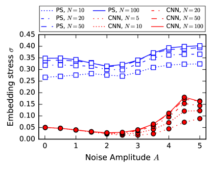
Figure 7: (Color online) The embedding stress $\sigma$ as a function of noise amplitude $A$, with scale $k=15$. Each dataset consists of $N$ images with varying angle $\theta_{i}$. The CNN method yields much lower stress embeddings than the PS method.

IV.3 Three dimensional manifold reconstruction task

Here we embed texture images from all three generating parameters shown in Fig. 3: the angle $0\leq\theta<\pi$, scale $5\leq k<15$, and noise amplitude $0.5\leq A<2$. We generate a dataset of $N=1000$ texture images by varying each parameter through $10$ equally spaced increments. As before, we determine the distances between images using CNN (Sec. III.1) and power spectrum (Sec. III.2) methods, then use MDS (Sec. III.3) to embed these distances into spaces of varying dimension $D^{\ast}$.

Figure 8 shows the embedding stress $\sigma$ as a function of embedding dimension $D^{\ast}$. We observe a much lower stress using the CNN distances. The stress $\sigma$ decays exponentially up to about $D^{\ast}=6$ and flattens soon after. That is, with $\approx 6$ descriptors per image, MDS has learned a representation of the texture images quite faithful to the CNN distances. Conversely, for the PS method, $\sigma$ decays very slowly with $D^{\ast}$, suggesting that there is no natural low-dimensional embedding manifold.

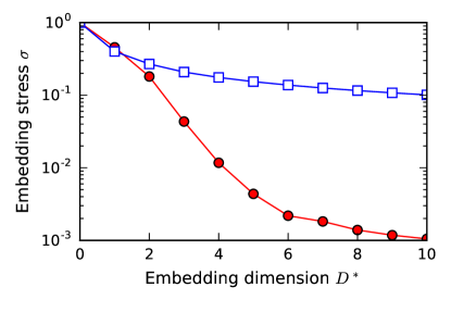
Figure 8: (Color online) The stress $\sigma$ as a function of embedding dimension $D^{\ast}$ for a dataset of $N=1000$ images with varying $A$, $k$, and $\theta$. Stress from the CNN method (red) decreases approximately exponentially for $D^{\ast}\lesssim 6$. Stress from the PS method (blue) decreases much more slowly. That is, the PS distances do not naturally embed into low dimensions.

The panels in Fig. 9 show the CNN method embeddings in a $D^{\ast}=3$ space. The generating parameters $A$, $k$, and $\theta$ emerge as a nonlinear coordinate system that spans a roughly conical solid in the embedding space. Column (a) of Figure 9 shows surfaces in which the noise amplitude $A$ is held fixed, and the parameters $\theta$ and $k$ are allowed to vary. For each $A$, the embedded points form an approximately conic surface. Cones with larger $A$ are nested inside of cones with smaller $A$. Column (b) of Figure 9 shows surfaces in which the scale $k$ is held fixed, allowing $A$ and $\theta$ to vary. Surfaces of constant $k$ are harder to describe, but resemble fragments of conic surfaces with varying angles. Surfaces with smaller $k$ are nested inside of ones with larger $k$. Column (c) of Figure 9 shows surfaces in which the angle $\theta$ is held fixed, allowing $A$ and $k$ to vary. Rotating to a top-down view (Fig. 10), one observes that $\theta$ is very well captured by the azimuthal angle of the cone structure.

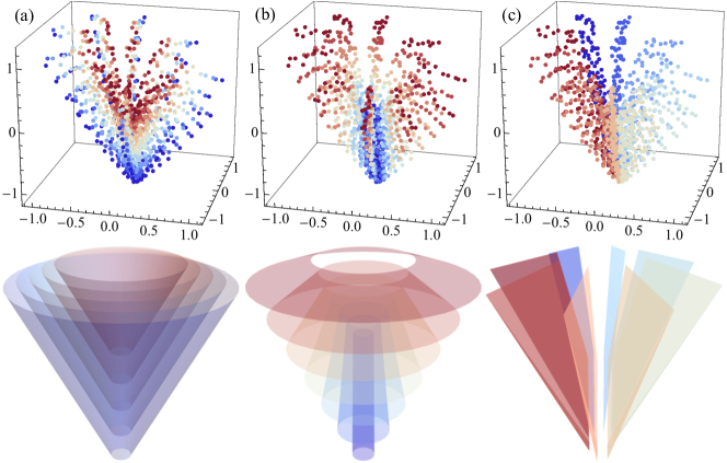
Figure 9: (Color online) The $D^{\ast}=3$ embedding of a dataset with $N=1000$ image of varying noise amplitude $A$, scale $k$, and angle $\theta$. Columns (a), (b), and (c) are colored by $A$, $k$, and $\theta$, respectively. For each column, the top panel shows the embedded points, and the bottom panel displays a schematic representation of surfaces with constant generating parameter.

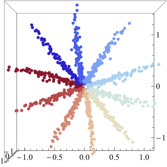
Figure 10: (Color online) Axis-aligned view of the $D^{\ast}=3$ embedding colored by angle $\theta$ (cf. Fig. 9), demonstrating strong correspondence with angles in the embedding space.

Figure 11 shows a 3-D projection of the $D^{\ast}=4$ embedding. In this projection, we observe that the generating parameters appear approximately as cylindrical coordinates. The noise parameter $A$ appears approximately linearly as a longitudinal coordinate.

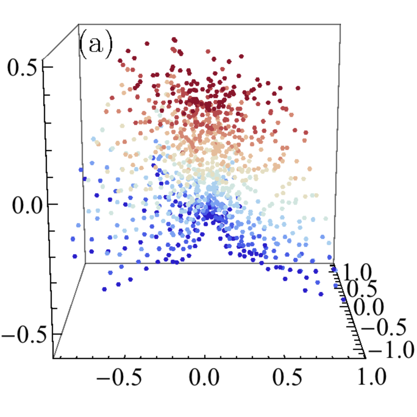
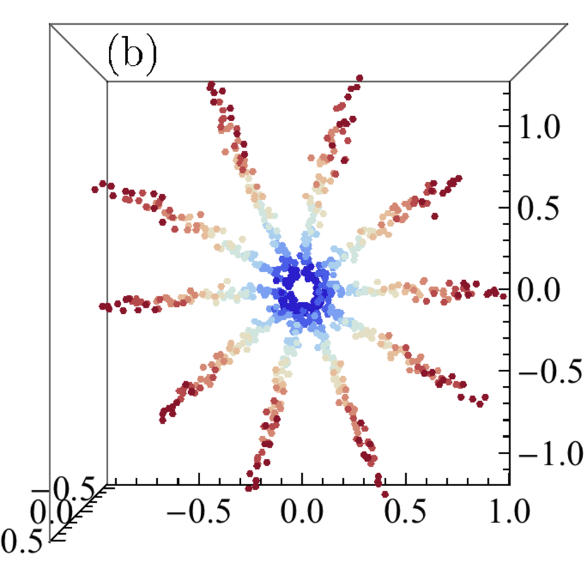
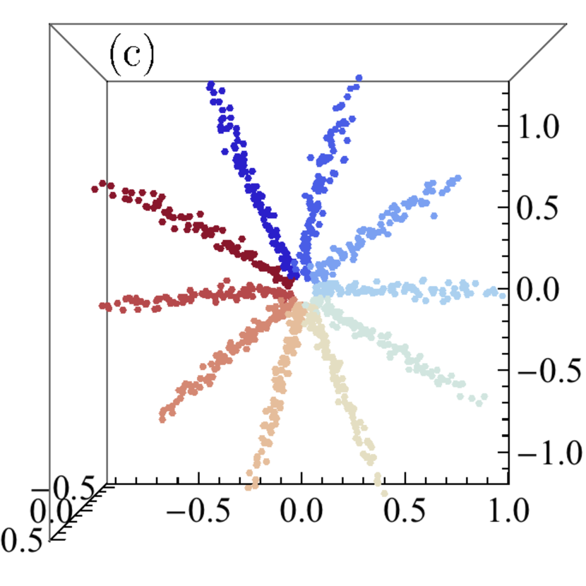
Figure 11: (Color online) The $D^{\ast}=4$ embedding of a dataset with $N=1000$ images of varying noise amplitude $A$, scale $k$, and angle $\theta$. Panels (a), (b), and (c) are colored by $A$, $k$, and $\theta$, respectively. To visualize the data, we select a 3-D projection that illustrates a decoupling of the generating parameters, in which they manifest as roughly cylindrical coordinates: $A$ maps to longitudinal height, $k$ to radius, and $\theta$ to azimuthal angle.

To quantitatively evaluate the quality of embeddings for general dimension $D^{\ast}$, we performed linear regression to model the parameters $A_{i}$ and $k_{i}$ for each embedding point $\hat{x}_{i}$:

$$\hat{A}_{i}=\beta_{A}\cdot\hat{x}_{i}+\gamma_{A}\,,$$ (11)

$$\hat{k}_{i}=\beta_{k}\cdot\hat{x}_{i}+\gamma_{k}\,.$$ (12)

The regression vectors $\beta_{p}$ and scalars $\gamma_{p}$ for $p\in\{A,k\}$ were found using ordinary least squares by minimizing $\sum_{i}(p_{i}-\hat{p}_{i})^{2}$. We then assess fit quality using the coefficient of determination,

$$R^{2}=1-\frac{\sum_{i}(p_{i}-\hat{p}_{i})^{2}}{\sum_{i}(p_{i}-\bar{p})^{2}},$$ (13)

where $\bar{p}=\sum_{i}p_{i}/N$. An $R^{2}$ value of $1$ indicates a perfectly linear relationship. Table 1 shows $R^{2}$ values for $k$ and $A$ in various embedding dimensions. In particular, $R^{2}\approx 1$ is achieved already with $D^{\ast}=4$ and higher-dimensional embeddings ($D^{\ast}>4$) yield only marginal increase in fit quality.

Embedding dimension $D^{\ast}$	2	3	4	5	6	10	50
$R^{2}$ for scale $k$	.532	.720	.901	.916	.916	.930	.980
$R^{2}$ for noise amplitude $A$	.183	.231	.908	.950	.951	.972	.983

Table 1: The coefficients of determination $R^{2}$ for linear regression models that map embedded points $\hat{x}_{i}$ to $k_{i}$ or $A_{i}$. For embedding dimensions $D^{\ast}\geq 4$, the linear models achieve $R^{2}$ values near the ideal of 1.

Figure 12 shows the $D^{\ast}=6$ embedding projected onto the two dimensions, $\{\beta_{k},\beta_{A}\}$, that best linearly model the noise amplitude and scale parameters. The scale and noise parameters are nearly orthogonal; the angle between $\beta_{k}$ and $\beta_{A}$ is

$$\theta=\arccos\left(\frac{\beta_{A}\cdot\beta_{k}}{\|\beta_{A}\|\|\beta_{k}\|}\right)=91.0\degree.$$ (14)

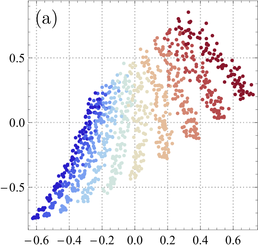
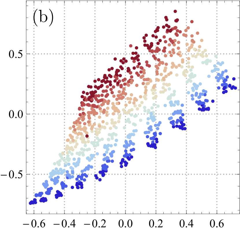
Figure 12: (Color online) The 2-D projection, colored by (a) scale and (b) noise amplitude, of the $D^{\ast}=6$ embedding of a dataset with $N=1000$ images of varying $A$, $k$, and $\theta$. This projection was selected using linear regression to find the two dimensions that best capture the scale $k$ and noise amplitude $A$ parameters.

V Discussion

The effectiveness of the PS on the angle reconstruction task (see Fig. 6) is best for moderate values of the noise, but weak outside of this window. Although we discussed the mechanisms at play, this result is at first counterintuitive; The images consist of perturbed sinusoidal stripes that coincide well the Fourier basis used by the PS. The performance of the CNN texture vector is much better, achieving high accuracy and consistent performance across the spectrum of noise. This can be attributed to several advantages of the CNN-based approach.

First, the CNN uses local filters as opposed to global modes. Global features can suffer from interference effects, where similar small scale features which appear at a large distances from each other can add together destructively. Local features do not suffer from this type of failure mode, and so are more robust to noisy variations in patterns. This is similar to advantages of compact support in wavelet approaches to signal processing, which are well studied Mallat (2008).

Second, compositions of convolutional filters and nonlinear activations represent very non-trivial correlations between the pixels within their receptive fields, so that individual neurons are sensitive to higher order statistics that are not captured in the PS representation. For example, higher order statistics can directly characterize complex features such as domain edge curvature.

Lastly, the pooling layers in the CNN operate similarly to coarse-graining in physics, and is designed to capture relevant system characteristics while discarding unimportant ones [AnexplicitcorrespondencebetweenthevariationalrenormalizationgroupanddeeplearningusingBoltzmannMachinesisdemonstratedin][]Mehta14. In the CNN, repeated convolutional and pooling operations effectively implement coarse-graining over multiple layers of abstraction. Features that appear in deeper layers (i.e. further from the input) of the CNN have a spatially larger receptive field, and are more robust to small changes of the input due to the coarse-graining. Thus, larger-scale CNN features are naturally insensitive to smaller-scale texture details, which we believe is key to microstructure analysis as well as computer vision tasks. A trade-off with deep neural networks is that it can be difficult to understand concretely what a particular activation in a CNN represents; however, this is an active area of research Erhan et al. (2010); Yosinski et al. (2015); Selvaraju et al. (2016).

VI Conclusions and future directions

We have introduced a method for unsupervised detection of the low-dimensional structure of a distribution of texture images using CNNs. We discuss the uses of this as a framework for the analysis of materials microstructure to learn dimensionality and topology of microstructure families using low-dimensional quantitative descriptions of microstructure. Compact microstructure characterization forms a platform for the construction of reduced order models that connect processing to microstructure, and microstructure to properties. This approach is applicable to small data sets, which is an important design factor in materials science and other disciplines where acquiring data can be expensive. In this work, we apply manifold learning to a synthetic dataset. This controlled context enables us to quantify the success of manifold learning. We anticipate that similar manifold learning approaches will prove effective for follow-on studies of real materials. For example, DeCost et al. recently demonstrated success in mapping the microstructures of ultra high carbon steels DeCost et al. (2017).

The method presented in this work is computationally efficient. In our Theano implementation, running on a single GPU, it takes about a millisecond to compute the distance between texture vectors that represent two images. MDS operates on all distance pairs, and thus scales quadratically with the size of the dataset. The MDS calculation on our full dataset of $10^{3}$ synthetic images (Sec. IV.3) completed in about 30 minutes. The dominant cost was the MDS embedding procedure, which took about 18 minutes. Calculating the $\approx 10^{6}/2$ texture vector distances took about 12 minutes.

A limitation of the transfer learning approach is that it requires a well-trained CNN with applicability to the target domain, which presently limits our analysis to 2-D micrographs. One path for improvement is to directly train CNNs on a large database of standardized microstructure images. Such a database could also be used to develop latent variable models (e.g. Kingma and Welling (2013)) that would reflect the microstructural generation process. These end-to-end models would enable direct inference of low-dimensional generating parameters and direct generation of new microstructure image samples.

The work of Ref. Ustyuzhaninov et al., 2016 suggests that, instead of using transfer learning on natural images, it may be possible to characterize microstructure textures using randomized CNNs. Specifically, Ustyuzhaninov et al. conclude that suitably structured random, shallow, multiscale networks can, in some cases, be used to generate higher quality textures than those generated from a trained CNN. However, Fig. 1 of Ref. Ustyuzhaninov et al., 2016 shows that the distance matrix generated from the trained CNN is closer to the identity compared to the distance matrix generated from the random network. This suggests that the trained CNN is a better starting point for comparing texture images. The capability of random networks to perform low-dimensional embeddings of microstructures remains an open question. The use of random networks suggests exciting opportunities to operate on other data modalities, e.g. three-dimensional microstructure data Rollett et al. (2007); Sundararaghavan and Zabaras (2005); Xu et al. (2014) and/or grain orientation data Adams et al. (1993); Humphreys (2001); Orme et al. (2016), both of which are outside the domain of natural image characterization.

Lastly, we consider the rotation group, which factors into microstructure analysis in at least two ways. Firstly, rotations appear through spatial transformations of the image plane. The standard CNN architecture does not explicitly incorporate such transformations. This is evident in the small but consistent biases in the angular reconstruction task (see Figs. 5 and 6). However, the relatively strong performance of the network on this task indicates that the network has implicitly learned approximate representations of the rotation group during the training procedure. A second way that the rotation group appears is in grain orientation data. CNNs designed to process RGB images do not directly represent the group structure of crystalline orientations. Further texture characterization work might explicitly incorporate the action of rotations, e.g. building upon Refs. Mallat, 2012; Cohen and Welling, 2014; Gens and Domingos, 2014; Dieleman et al., 2016; Cohen and Welling, 2016.

Appendix A Attribution of microstructure images

The images appearing in Fig. 1 are released in the public domain, and available online. Permanent links are as follows. Top row, from left to right:

1. https://commons.wikimedia.org/w/index.php?title=File:Gailbach-Tonalit.jpg&oldid=179586143.

2. https://commons.wikimedia.org/w/index.php?title=File:PearliteSph3.jpg&oldid=149930090.

3. https://commons.wikimedia.org/w/index.php?title=File:Martensit.jpg&oldid=144193548.

4. https://commons.wikimedia.org/w/index.php?title=File:Lamine316L.jpg&oldid=66965939.

Bottom row, from left to right:

1. https://commons.wikimedia.org/w/index.php?title=File:Microstructure_of_rolled_and_annealed_brass;_magnification_400X.jpg&oldid=144992203.

2. https://commons.wikimedia.org/w/index.php?title=File:Ferrite-perlite-steel-A285.jpeg&oldid=140529933.

3. https://commons.wikimedia.org/w/index.php?title=File:Pearlite1.jpg&oldid=184321025.

4. https://commons.wikimedia.org/w/index.php?title=File:Feuerverzinkte_Oberfl%C3%A4che.jpg&oldid=140580291

References

- Kumar et al. (2006) H. Kumar, C. Briant, and W. Curtin, Mech. Mater. 38, 818 (2006).
- Ostoja-Starzewski (2007) M. Ostoja-Starzewski, Microstructural randomness and scaling in mechanics of materials (CRC Press, 2007).
- Wang and Pan (2008) M. Wang and N. Pan, Mater. Sci. Eng. R-Rep. 63, 1 (2008).
- Fullwood et al. (2010) D. T. Fullwood, S. R. Niezgoda, B. L. Adams, and S. R. Kalidindi, Prog. Mater. Sci. 55, 477 (2010).
- Torquato (2010) S. Torquato, Annu. Rev. Mater. Res. 40, 101 (2010).
- Rajan (2013) K. Rajan, Informatics for materials science and engineering: data-driven discovery for accelerated experimentation and application (Butterworth-Heinemann, 2013).
- Kalidindi (2015) S. R. Kalidindi, Int. Mater. Rev. 60, 150 (2015).
- Lookman et al. (2016) T. Lookman, F. J. Alexander, and K. R. (Eds.), Information Science for Materials Discovery and Design, edited by K. R. Turab Lookman, Francis J. Alexander (Springer International Publishing, 2016).
- Voyles (2017) P. M. Voyles, Curr. Opin. Solid State Mater. Sci. 21, 141 (2017), materials Informatics: Insights, Infrastructure, and Methods.
- Xue et al. (2016) D. Xue, P. V. Balachandran, J. Hogden, J. Theiler, D. Xue, and T. Lookman, Nat. Commun. 7, 11241 (2016).
- Kalidindi et al. (2011) S. R. Kalidindi, S. R. Niezgoda, and A. A. Salem, JOM 63, 34 (2011).
- Liu et al. (2013) Y. Liu, M. S. Greene, W. Chen, D. A. Dikin, and W. K. Liu, Comput. Aided Des. 45, 65 (2013).
- Niezgoda et al. (2013) S. R. Niezgoda, A. K. Kanjarla, and S. R. Kalidindi, Integr. Mater. Manuf. Innov. 2, 3 (2013).
- Jiao et al. (2007) Y. Jiao, F. H. Stillinger, and S. Torquato, Phys. Rev. E 76, 031110 (2007).
- Fullwood et al. (2008) D. T. Fullwood, S. R. Niezgoda, and S. R. Kalidindi, Acta Mater. 56, 942 (2008).
- Jiao et al. (2009) Y. Jiao, F. H. Stillinger, and S. Torquato, Proc. Natl. Acad. Sci. USA 106, 17634 (2009).
- Chen et al. (2014) D. D. Chen, Q. Teng, X. He, Z. Xu, and Z. Li, Phys. Rev. E 89, 013305 (2014).
- Jiao et al. (2010a) Y. Jiao, F. H. Stillinger, and S. Torquato, Phys. Rev. E 81, 011105 (2010a).
- Jiao et al. (2010b) Y. Jiao, F. H. Stillinger, and S. Torquato, Phys. Rev. E 82, 011106 (2010b).
- Gommes et al. (2012a) C. J. Gommes, Y. Jiao, and S. Torquato, Phys. Rev. E 85, 051140 (2012a).
- Gommes et al. (2012b) C. J. Gommes, Y. Jiao, and S. Torquato, Phys. Rev. Lett. 108, 080601 (2012b).
- Niezgoda et al. (2008) S. Niezgoda, D. Fullwood, and S. Kalidindi, Acta Mater. 56, 5285 (2008).
- Zachary and Torquato (2011) C. E. Zachary and S. Torquato, Phys. Rev. E 84, 056102 (2011).
- Gerke et al. (2014) K. M. Gerke, M. V. Karsanina, R. V. Vasilyev, and D. Mallants, Europhys. Lett. 106, 66002 (2014).
- Xu et al. (2014) H. Xu, D. A. Dikin, C. Burkhart, and W. Chen, Comput. Mater. Sci. 85, 206 (2014).
- Lecun et al. (1998) Y. Lecun, L. Bottou, Y. Bengio, and P. Haffner, Proc. IEEE 86, 2278 (1998).
- Krizhevsky et al. (2012) A. Krizhevsky, I. Sutskever, and G. E. Hinton, in Advances in Neural Information Processing Systems 25, edited by F. Pereira, C. J. C. Burges, L. Bottou, and K. Q. Weinberger (Curran Associates, Inc., 2012) pp. 1097–1105.
- Simonyan and Zisserman (2014) K. Simonyan and A. Zisserman, “Very deep convolutional networks for large-scale image recognition,” (2014), arXiv:1409.1556 [cs.CV] .
- Szegedy et al. (2015) C. Szegedy, W. Liu, Y. Jia, P. Sermanet, S. Reed, D. Anguelov, D. Erhan, V. Vanhoucke, and A. Rabinovich, in The IEEE Conference on Computer Vision and Pattern Recognition (CVPR) (2015).
- He et al. (2016) K. He, X. Zhang, S. Ren, and J. Sun, in The IEEE Conference on Computer Vision and Pattern Recognition (CVPR) (2016).
- LeCun et al. (2015) Y. LeCun, Y. Bengio, and G. E. Hinton, Nature 521, 436 (2015).
- Hao et al. (2012) T. Hao, T. Raiko, A. Ilin, and J. Karhunen, in Artif. Neural Networks Mach. Learn. – ICANN 2012, Lecture Notes in Computer Science, Vol. 7553, edited by A. E. Villa, W. Duch, P. Érdi, F. Masulli, and G. Palm (Springer Berlin Heidelberg, 2012) pp. 124–131.
- Kivinen and Williams (2012) J. Kivinen and C. Williams, in Proceedings of the Fifteenth International Conference on Artificial Intelligence and Statistics, Proceedings of Machine Learning Research, Vol. 22, edited by N. D. Lawrence and M. Girolami (PMLR, 2012) pp. 638–646.
- Luo et al. (2013) H. Luo, P. L. Carrier, A. Courville, and Y. Bengio, in Proceedings of the Sixteenth International Conference on Artificial Intelligence and Statistics, Proceedings of Machine Learning Research, Vol. 31, edited by C. M. Carvalho and P. Ravikumar (PMLR, 2013) pp. 415–423.
- Gao and Roth (2014) Q. Gao and S. Roth, in Struct. Syntactic, Stat. Pattern Recognit., Lecture Notes in Computer Science, Vol. 8621, edited by P. Fränti, G. Brown, M. Loog, F. Escolano, and M. Pelillo (Springer Berlin Heidelberg, 2014) pp. 434–443.
- Theis and Bethge (2015) L. Theis and M. Bethge, in Advances in Neural Information Processing Systems 28, edited by C. Cortes, N. D. Lawrence, D. D. Lee, M. Sugiyama, and R. Garnett (Curran Associates, Inc., 2015) pp. 1927–1935.
- Gatys et al. (2015) L. Gatys, A. S. Ecker, and M. Bethge, in Advances in Neural Information Processing Systems 28, edited by C. Cortes, N. D. Lawrence, D. D. Lee, M. Sugiyama, and R. Garnett (Curran Associates, Inc., 2015) pp. 262–270.
- Gatys et al. (2016) L. A. Gatys, A. S. Ecker, and M. Bethge, in The IEEE Conference on Computer Vision and Pattern Recognition (CVPR) (2016).
- Russakovsky et al. (2015) O. Russakovsky, J. Deng, H. Su, J. Krause, S. Satheesh, S. Ma, Z. Huang, A. Karpathy, A. Khosla, M. Bernstein, A. C. Berg, and L. Fei-Fei, Int. J. Comput. Vision 115, 211 (2015).
- DeCost et al. (2017) B. L. DeCost, T. Francis, and E. A. Holm, Acta Materialia 133, 30 (2017).
- Sundararaghavan and Zabaras (2005) V. Sundararaghavan and N. Zabaras, Comput. Mater. Sci. 32, 223 (2005).
- DeCost and Holm (2015) B. L. DeCost and E. A. Holm, Comput. Mater. Sci. 110, 126 (2015).
- Kalinin et al. (2015) S. V. Kalinin, B. G. Sumpter, and R. K. Archibald, Nat. Mater. 14, 973 (2015).
- Liu et al. (2015) R. Liu, A. Kumar, Z. Chen, A. Agrawal, V. Sundararaghavan, and A. Choudhary, Sci. Rep. 5, 11551 (2015).
- Bostanabad et al. (2016) R. Bostanabad, A. T. Bui, W. Xie, D. W. Apley, and W. Chen, Acta Mater. 103, 89 (2016).
- Chowdhury et al. (2016) A. Chowdhury, E. Kautz, B. Yener, and D. Lewis, Comput. Mater. Sci. 123, 176 (2016).
- Orme et al. (2016) A. D. Orme, I. Chelladurai, T. M. Rampton, D. T. Fullwood, A. Khosravani, M. P. Miles, and R. K. Mishra, Comput. Mater. Sci. 124, 353 (2016).
- He et al. (2015) K. He, X. Zhang, S. Ren, and J. Sun, in The IEEE International Conference on Computer Vision (ICCV) (2015) pp. 1026–1034.
- Goodfellow et al. (2016) I. Goodfellow, Y. Bengio, and A. Courville, Deep Learning (MIT Press, 2016) http://www.deeplearningbook.org.
- Theano Development Team (2016) Theano Development Team, “Theano: A Python framework for fast computation of mathematical expressions,” (2016), arXiv:1605.02688 [cs.SC] .
- Dieleman et al. (2015) S. Dieleman, J. Schlüter, C. Raffel, E. Olson, S. K. Sønderby, D. Nouri, D. Maturana, M. Thoma, E. Battenberg, J. Kelly, et al., “Lasagne: First release.” (2015).
- Kruskal (1964) J. B. Kruskal, Psychometrika 29, 1 (1964).
- Borg and Groenen (2005) I. Borg and P. J. F. Groenen, Modern Multidimensional Scaling: Theory and Applications, Springer Series in Statistics (Springer-Verlag New York, 2005).
- Franklin (2008) J. Franklin, Math. Intell. 27, 83 (2008).
- Roweis and Saul (2000) S. T. Roweis and L. K. Saul, Science 290, 2323 (2000).
- Tenenbaum et al. (2000) J. B. Tenenbaum, V. d. Silva, and J. C. Langford, Science 290, 2319 (2000).
- Pedregosa et al. (2011) F. Pedregosa, G. Varoquaux, A. Gramfort, V. Michel, B. Thirion, O. Grisel, M. Blondel, P. Prettenhofer, R. Weiss, V. Dubourg, J. Vanderplas, A. Passos, D. Cournapeau, M. Brucher, M. Perrot, and E. Duchesnay, J. Mach. Learn. Res. 12, 2825 (2011).
- De Leeuw (1977) J. De Leeuw, in Recent Developments in Statistics, edited by J. R. Barra, F. Brodeau, G. Romier, and B. van Cutsem (Verlag: North-Holland, 1977) pp. 133–145.
- Perlin (1985) K. Perlin, SIGGRAPH Comput. Graph. 19, 287 (1985).
- Mallat (2008) S. Mallat, A Wavelet Tour of Signal Processing, Third Edition: The Sparse Way, 3rd ed. (Academic Press, 2008).
- Mehta and Schwab (2014) P. Mehta and D. J. Schwab, “An exact mapping between the Variational Renormalization Group and Deep Learning,” (2014), arXiv:1410.3831 [cs.CV] .
- Erhan et al. (2010) D. Erhan, A. Courville, and Y. Bengio, Understanding Representations Learned in Deep Architectures, Tech. Rep. 1355 (Université de Montréal/DIRO, 2010).
- Yosinski et al. (2015) J. Yosinski, J. Clune, A. Nguyen, T. Fuchs, and H. Lipson, in Deep Learning Workshop, International Conference on Machine Learning (ICML) (2015).
- Selvaraju et al. (2016) R. R. Selvaraju, A. Das, R. Vedantam, M. Cogswell, D. Parikh, and D. Batra, “Grad-CAM: Why did you say that? Visual Explanations from Deep Networks via Gradient-based Localization,” (2016), arXiv:1610.02391 [cs.CV] .
- Kingma and Welling (2013) D. P. Kingma and M. Welling, “Auto-Encoding Variational Bayes,” (2013), arXiv:1312.6114 [stat.ML] .
- Ustyuzhaninov et al. (2016) I. Ustyuzhaninov, W. Brendel, L. A. Gatys, and M. Bethge, “Texture synthesis using shallow convolutional networks with random filters,” (2016), arXiv:1606.00021 [cs.CV] .
- Rollett et al. (2007) A. Rollett, S.-B. Lee, R. Campman, and G. Rohrer, Annu. Rev. Mater. Res. 37, 627 (2007).
- Adams et al. (1993) B. Adams, S. Wright, and K. Kunze, Metall. Trans. A 24, 819 (1993).
- Humphreys (2001) F. J. Humphreys, J. Mater. Sci. 36, 3833 (2001).
- Mallat (2012) S. Mallat, Commun. Pure Appl. Math. 65, 1331 (2012).
- Cohen and Welling (2014) T. S. Cohen and M. Welling, “Transformation properties of learned visual representations,” (2014), arXiv:1412.7659 [cs.LG] .
- Gens and Domingos (2014) R. Gens and P. M. Domingos, in Advances in Neural Information Processing Systems 27, edited by Z. Ghahramani, M. Welling, C. Cortes, N. D. Lawrence, and K. Q. Weinberger (Curran Associates, Inc., 2014) pp. 2537–2545.
- Dieleman et al. (2016) S. Dieleman, J. D. Fauw, and K. Kavukcuoglu, in Proceedings of The 33rd International Conference on Machine Learning, Proceedings of Machine Learning Research, Vol. 48, edited by M. F. Balcan and K. Q. Weinberger (PMLR, 2016) pp. 1889–1898.
- Cohen and Welling (2016) T. Cohen and M. Welling, in Proceedings of The 33rd International Conference on Machine Learning, Proceedings of Machine Learning Research, Vol. 48, edited by M. F. Balcan and K. Q. Weinberger (PMLR, 2016) pp. 2990–2999.