Modularity promotes epidemic recurrence

Abstract

The long-term evolution of epidemic processes depends crucially on the structure of contact networks. As empirical evidence indicates that human populations exhibit strong community organization, we investigate here how such mesoscopic configurations affect the likelihood of epidemic recurrence. Through numerical simulations on real social networks and theoretical arguments using spectral methods, we demonstrate that highly contagious diseases that would have otherwise died out rapidly can persist indefinitely for an optimal range of modularity in contact networks.

Infectious diseases continue to remain among the major causes of human mortality worldwide, despite considerable progress in their treatment and management WHO2004 . In recent decades, periodically reemerging epidemics have posed a significant challenge to public health globally Morens04 ; Fauci05 . Various causative factors for such re-emergence have been suggested, including zoonotic encounters Jones2008 ; Morse2012 , environmental degradation Dobson2001 and periodic variations in climate Kovats03 ; Sultan05 . However, such explanations are crucially dependent on exogenous factors specific to a particular outbreak. A more general framework for explaining the recurrent pattern of epidemics should involve endogenous properties of contagion spreading between individuals in a population. Critical determinants of such processes include the properties of the contact network that allow an infection to propagate Kitsak2010 ; Goltsev2012 ; PastorSatorras2015 . More generally, explaining how long-term recurrence can arise in dynamical systems coupled by non-local diffusive interactions can contribute to understanding persistence in non-equilibrium systems Schehr2007 ; Majumdar2010 ; Bray2013 .

A prominent topological characteristic of social networks is their modular nature Wasserman94 ; Girvan02 ; Onnela07 ; Nematzadeh2014 : it is possible to identify communities with a high density of connections between their members, as compared to those between members of different communities. Earlier studies have shown that diseases are less likely to become established in networks that are strongly modular Liu05 ; Huang06 ; Huang07 ; Zhao07 ; Griffin12 . It has also been shown that immunization in modular networks is more effective if individuals bridging communities, rather than the most highly connected individuals, are preferentially targeted Masuda09 ; Salathe10 . However, the impact of such mesoscopic organization of populations on the eventual fate of a contagion has remained relatively unexplored. This is surprising given that the long-term outcome of an epidemic breakout is critical from the perspective of disease eradication and control. In particular, the study of persistence time of a disease Earn98 reveals the existence of a critical population size Bartlett57 below which an epidemic, after an initial phase of rapid growth, becomes extinct due to the paucity of susceptible individuals. Theoretical studies of disease persistence typically consider homogeneous random mixing in populations, and it is an open question as to whether the presence of modular topological organization in contact networks, as seen in human societies, can significantly affect the critical population size for a highly infectious disease.

In this paper, we demonstrate the key role played by the mesoscopic structure of the contact network, viz., its modular organization, in the dynamics of epidemics at long time-scales. We specifically show that highly infectious diseases that would have otherwise died out rapidly can persist indefinitely for an optimal range of modularity. The critical role played by the mesoscopic structural organization in this phenomenon is established by implementing stochastic contagion spreading dynamics on an ensemble of empirical social networks, as well as on contact network models whose modularity can be tuned. We observe that modularity differentially affects the fate of infections depending on their contagiousness, quantified by the basic reproduction number $R_{0}$, i.e., the average number of secondary infections resulting from a single infected agent in the initial stage of the epidemic when almost the entire population is susceptible Anderson91 . Thus, while epidemics with lower $R_{0}$ can persist in populations exhibiting relatively homogeneous contact networks, those with higher $R_{0}$ can survive only in networks with strong modular organization. This has obvious public health policy implications, especially in designing effective intervention strategies for countering recurrent epidemics.

The quantitative framework for understanding recurrence-driven persistence of epidemics is provided by the SIRS compartmental model of epidemic spreading Anderson91 . A population of $N$ agents (represented by the nodes of a network) is composed of susceptible ($S$), infected ($I$) and recovered ($R$) individuals, whose numbers vary with the progress of the epidemic over time. Each link between a pair of nodes is a contact along which infection can propagate, with the rate of infection transmission from an infected to a susceptible agent being $\beta$. Infected agents are assumed to recover at a rate $\gamma=1/\tau_{I}$, where $\tau_{I}$ is the average duration of the infection. A recovered agent has temporary immunity to the infection for a period whose average value is $\tau_{R}$, after which it becomes susceptible again. Thus, the transition from recovered state to susceptible state occurs at a rate $\mu=1/\tau_{R}$. Note that limiting cases of the SIRS model yield other well-known models such as the SI ($\tau_{I}\rightarrow\infty$), SIR ($\tau_{R}\rightarrow\infty$) and SIS ($\tau_{R}\rightarrow 0$), which have all been used in studies of contagion propagation. In a contact network with average degree (i.e., links per node) $k$, the basic reproduction number for an SIRS process can be approximated as $R_{0}\simeq k\beta\tau_{I}$ Keeling00 .

To perform stochastic simulations of contagion propagation on a contact network, we have used the Gillespie direct algorithm Gillespie77 . The rates of $I\rightarrow R$ and $R\rightarrow S$ events are not constant, but depend on the time elapsed after infection ($\Delta t_{I}$) and recovery ($\Delta t_{R}$) respectively, viz., $\gamma={\rm exp}(\eta(\Delta t_{I}-\tau_{I}))$ and $\mu={\rm exp}(\eta(\Delta t_{R}-\tau_{R}))$ where $\eta$ governs the nature of the distributions of durations of infection and recovery of individuals. This is to take into account the fact that in reality the rate at which an individual recovers in a given time interval is initially small but increases over time, corresponding to the infectious period distribution being less skewed than an exponential distribution (which would have been obtained had the recovery rate been assumed to be constant in time) Keeling97 ; Lloyd01 . We carry out simulations for durations (typically $>10^{3}$ time units) that are much longer than any of the time-scales ($\tau_{I}$, $\tau_{R}$) governing the dynamics of the SIRS model. While results shown here are for $\tau_{I}=5,\tau_{R}=10$, we have explicitly verified that qualitatively similar behavior is seen for different choices for these parameters.

Figure 1: (color online). (a) Visualization of the largest connected component of the social network in a village of southern India comprising $N=1151$ individuals (contact data from Ref. Banerjee13 ), on which we simulate contagion propagation. Nodes are colored according to the community they belong to, obtained using a spin glass energy minimization method Reichardt06 . (b-c) The time-evolution of the fraction of infected individuals, $f_{inf}$, for a simulated epidemic with basic reproduction number $R_{0}=7$, started by infecting a randomly chosen 1% of the population in (b) the empirical contact network shown above, and (c) a degree-preserved randomization of the same network. Note that the contagion is persistent for an extremely long period ($>10^{3}$ time units) in the empirical network compared to the randomized network where community structure is absent. (d) The probability that an epidemic persists for longer than a specific duration in the empirical contact network (red circles) and corresponding degree-preserved randomized networks (blue squares, averaged over 100 network realizations) shown as a function of the basic reproductive number $R_{0}$ of the epidemic. When the contagion is more infectious ($R_{0}>5$), the epidemic is more likely to be persistent in the empirical network compared to the randomized ones. (e) The role of modularity (measured by $Q$) in increasing the probability of persistence of an epidemic, measured as the Jensen-Shannon divergence between the persistence probability distributions for empirical contact networks for 75 different villages and that of corresponding degree-preserved randomized networks. The linear correlation coefficient for correlation between $Q$ and $JSD$ is $0.89$ ($p$-value $=0$).

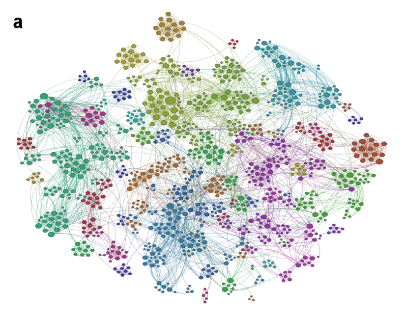
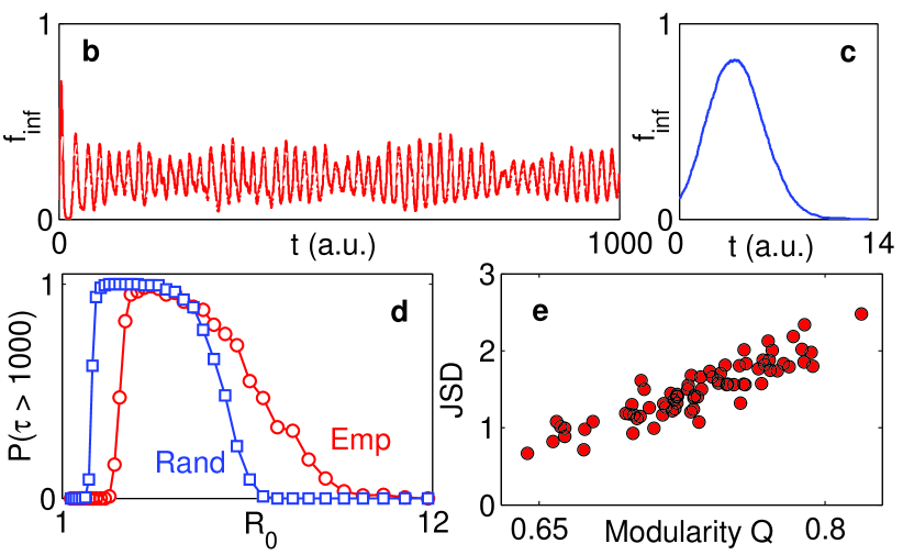
We first establish the crucial role played by modularity in the long-term behavior of an epidemic by simulating contagion spreading on a set of empirical social networks. We have reconstructed these networks from detailed information on social interactions between individuals belonging to 75 villages in southern India (using data from Ref. Banerjee13 ). Fig. 1 (a) shows a representative network corresponding to one of the larger villages where the different modules identified by a community detection algorithm Reichardt06 are indicated. We observe that initiating an epidemic in the network results in the contagion surviving indefinitely over a range of simulation parameters [Fig. 1 (b)]. However, if the network is randomized so as to remove the modular structure the contagion is extinguished rapidly in the same parameter regime [Fig. 1 (c)]. Fig. 1 (d) shows how the persistence behavior of the epidemic, measured in terms of the duration $\tau$ for which the infection survives in the population, differs between the empirical network and the corresponding randomized network ensemble - the former being more likely to exhibit persistence of highly infectious (viz., $R_{0}>5$) contagia than the latter. As the randomized networks have a degree sequence identical to the empirical network, it suggests that the enhanced persistence of the epidemic in the latter is a consequence of its modular organization. This is further supported by observing that the persistence behavior is enhanced if we reduce only the inter-modular connections in an empirical network (which effectively increases its modularity supp ). Indeed, a quantitative relation between persistence behavior and modularity can be obtained by showing how the difference in the persistence probability distributions for empirical and randomized networks vary as a function of the modularity ($Q$) of the empirical networks Newman2006 . This difference is measured by the Jensen-Shannon divergence Lin1991 , defined for a pair of discrete probability distributions $X$ and $Y$ as:

$$JSD(X,Y)=\frac{1}{2}\Sigma_{i}\left(X_{i}\ln\frac{X_{i}}{Z_{i}}+Y_{i}\ln\frac{Y_{i}}{Z_{i}}\right),$$

where $Z=\frac{1}{2}(X+Y)$. Fig. 1 (e) shows that JSD increases almost linearly with $Q$ of the contact network, establishing the critical role of modularity in enhancing the persistence of highly infectious epidemics.

Figure 2: (color online). (a-c) Adjacency matrices of the contact network model shown for different values of the modularity parameter $r=\rho_{out}/\rho_{in}\in[0,1]$, which is the ratio of inter-modular to intra-modular connection density for a fixed average degree $k$. Starting from a collection of isolated clusters (a, $r=0$), by increasing $r$ we obtain modular networks (b, $r=0.1$) eventually arriving at a homogeneous network (c, $r=1$). (d) The probability of persistence for an epidemic (viz., duration $\tau>10^{3}$ time units) having a basic reproduction number $R_{0}=6$ in a modular network of $N=1000$ agents ($k=12$), grouped into $M=20$ modules peaks in an optimal range of $r$, independent of the heterogeneity in community sizes (measured by their standard deviation $\sigma$). Increasing the number of modules $M$ enhances the observed persistence behavior supp . (e) The probability of persistence ($\tau>10^{4}$) of an epidemic in a modular network ($N=1024$, $M=64$, $\sigma=0$, $k=12$) as a function of $R_{0}$ and $r$. In a homogeneous network ($r=1$), highly infectious contagia (viz., $R_{0}>5$) rapidly infect almost all agents and become extinct. Systems with almost isolated modules ($r\rightarrow 0$) also exhibit short-lived epidemics as a local outbreak in one module is unable to transfer to the others. However, for an optimally modular network ($r\sim 10^{-3}$), epidemics with high values of $R_{0}$ can become recurrent and persist in populations for extremely long times.

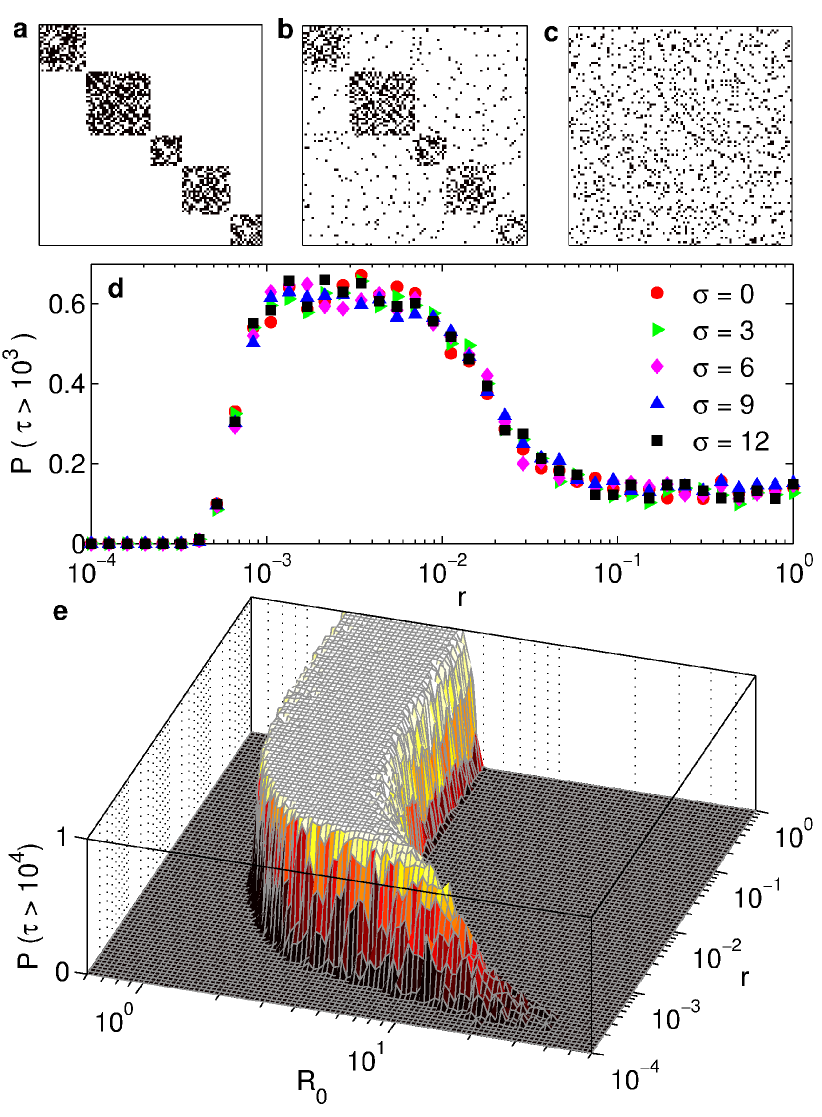
In order to investigate the mechanism by which community organization affects the long-term dynamics of epidemics, we consider an ensemble of model contact networks whose modularity can be tuned Pan09 . Each network is constructed such that the $N$ nodes (representing agents) comprising the system are arranged into $M$ modules that can have varying sizes. The size distribution has a Gaussian form with a mean size $\langle n\rangle(=N/M)$ and standard deviation, $\sigma$, which is a free parameter that determines the heterogeneity in community sizes Menon15 . Unlike most earlier studies of epidemic dynamics on community-structured networks, the modular nature of this network model can be varied continuously by tuning the ratio of inter- to intra-modular connectivity, $r=\rho_{out}/\rho_{in}\in[0,1]$ without changing the average degree $k$ of the nodes [Fig. 2 (a-c)].

Fig. 2 (d) shows the probability that a highly infectious contagion ($R_{0}=6$) survives for long times in contact networks as a function of their modular character, parameterized by $r$. We observe that there is an optimal range of $r$ over which the epidemic becomes persistent, independent of the level of heterogeneity in module sizes. This is consistent with the results obtained for empirical social networks above, as the modular nature of the contact network is most prominent over this range while still keeping the entire network connected. Decreasing $r$ further makes the modules effectively isolated from each other, preventing a local epidemic outbreak from spreading to the rest of the population. On increasing $r$ the modular structure become less prominent and the epidemic rapidly spreads through the relatively homogeneous network. Both scenarios result in the extinction of the infection in the population within a short duration.

To see how this relation between persistence and modularity is affected by the contagiousness of the epidemic - an important intrinsic property of its dynamics - in Fig. 2 (e) we look at the joint dependence of the probability that the epidemic persists for long times on $R_{0}$ and $r$. The contagion results in an epidemic when $R_{0}>1$, and in the extreme limit where no modularity is apparent (i.e., the completely homogeneous network obtained for $r=1$) it will persist in the population only if it propagates sufficiently slowly, so as to allow recovered agents to become susceptible again while the infection is still present in the system. Thus, we observe the probability of survival of the contagion to be high only for epidemics with low contagiousness ($R_{0}<5$) at the limit $r=1$, which can be explained quantitatively in terms of a solution of a delay difference equation supp . The range of $R_{0}$ over which the epidemic is seen to become persistent remains effectively unchanged as $r$ is decreased until the network becomes sufficiently modular [around $r\sim 10^{-2}$ in Fig. 2 (e)], after which we observe a gradual shift of the persistence range towards higher values of $R_{0}$. However, if $r$ is decreased further, the modules eventually become isolated [$r\gtrsim 10^{-4}$ in Fig. 2 (e)]. This results in rapid extinction of any epidemic that is initiated, as the contagion is unable to spread through the entire population regardless of $R_{0}$.

To investigate in more detail the mechanism by which the lifetime $\tau$ of an epidemic with high $R_{0}$ diverges in optimally modular networks, we can examine how the nature of its distribution $P(\tau)$ changes upon varying the parameter $r$ controlling the modularity of the network. Decreasing $r$ from $1$, as we approach the range where persistence is observed the distribution becomes bimodal, splitting into two branches supp . The lower branch corresponds to epidemic events confined within a community, where they spread rapidly and become extinct when no further susceptible agents are available. By contrast, the upper branch is peaked around a value that diverges with decreasing $r$ and represents realizations where the epidemic is able to successfully break out from the module in which it started, subsequently spreading from one community to another.

Figure 3: (color online). (a) Variation of the inverse of the smallest finite eigenvalue of the Laplacian for a modular network, representing the global diffusion time-scale, with the parameter $r$. (b) The Laplacian spectral gap, corresponding to the time-scale separation between intra- and inter-modular processes, shown as a function of $r$. The different curves coincide on scaling with number of modules $M$. The ratio of the time-scale separation (scaled by $M$) and global time-scale is shown in (c), which exhibits a peak in the region corresponding to optimal modularity for epidemic persistence. The symbols represent networks having different values of $M$ [see key in (c)]. For all results shown here $N=1024$ and $k=12$.

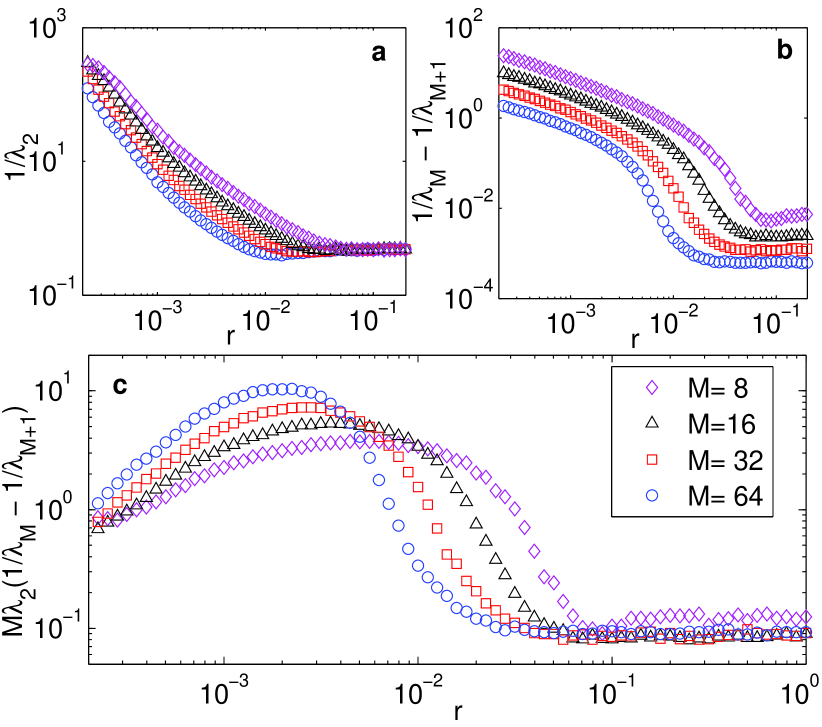
Thus, the key for understanding epidemic persistence in networks having community organization is the occurrence of spreading involving different time-scales in modular contact networks. This can be understood analytically in terms of a diffusion process defined on such networks with the probability of transmission from agent $i$ to $j$ in a single time step being $p_{ij}=A_{ij}/k_{i}$, where $A$ is the network adjacency matrix (i.e., $A_{ij}=1$, if $i,j$ are connected and $=0$, otherwise) and $k_{i}$ is the degree of $i$-th agent. The transmission probability matrix p is related to the normalized Laplacian of the network, ${\mathscr{L}}=$ I$-$D${}^{\frac{1}{2}}$pD${}^{-\frac{1}{2}}$ where I is the identity matrix and D is a diagonal matrix with $D_{ii}=k_{i}$. The Laplacian spectrum for undirected networks (as considered here) comprises non-negative real eigenvalues $\lambda_{1}=0\leq\lambda_{2}\leq\lambda_{3}....\lambda_{N}$. The reciprocal of the eigenvalues are related to time-scales for diffusion occurring over different ranges, with the smallest non-zero eigenvalue ($\lambda_{2}$ for a connected network) corresponding to global diffusion, i.e., the contagion spreading through the entire network. Fig. 3 (a) shows that this time decreases with increasing $r$ as the network becomes more homogeneous. The role of the modular organization becomes clear if we focus on the gap in the eigenvalue spectrum between $\lambda_{M}$ and $\lambda_{M+1}$ for a network with $M$ modules, that is related to the difference in the time-scales of fast intra-modular processes and slow inter-modular processes Pan09 . Fig. 3 (b) shows that this spectral gap also decreases with increasing $r$, i.e., the difference between the time-scales also increases. The occurrence of persistence in an optimal range of modularity is explained by looking at the ratio of the spectral gap to the global diffusion time-scale shown in Fig. 3 (c). This quantity peaks for an intermediate value of $r$ (between $10^{-3}$ and $10^{-2}$ in Fig. 3 (c)), where the epidemic propagates sufficiently rapidly so as not to become extinct before being able to hop from one module to another. Nonetheless, the global diffusion time is long enough such that when the epidemic returns after circulating around the network, a sufficient number of agents would have become susceptible for the epidemic to continue.

To conclude, we have shown that there is an optimal range of modularity of the contact network for which highly contagious diseases can persist indefinitely in the population. Our work has potential ramifications for the long-term management of contagious diseases, suggesting that determination of the critical population size required for epidemics to become recurrent has to necessarily take into account the mesoscopic organization of the social network. In particular, it suggests that interventions such as quarantine that isolate local communities from each other (thereby increasing modularity) can have very different efficacies from the perspective of the long-term recurrence of a disease depending on its $R_{0}$.

We thank Shakti N. Menon, Raj K. Pan and Rajeev Singh for helpful discussions, R. Janaki for assistance and IMSc for providing computational resources. This work was supported in part by IMSc Complex Systems Project (XII Plan) funded by the Department of Atomic Energy, Government of India.

Data description. Empirical social contact networks among individuals residing in each of 75 villages located in southern Karnataka, a state in the south of India, were reconstructed from detailed information about the relationships of the villagers with each other data1 . This data was collected through a survey carried out as part of a study on the operational feasibility of a microfinance institution in these villages Banerjee . The different types of relations between the surveyed individuals that were recorded included kinship, social engagement, mentoring, visiting homes, borrowing and lending money or essential items, etc. We assume that the existence of any kind of relation between a pair of individuals provides a pathway for the transmission of the contagion. Furthermore, from the perspective of spreading of a pathogen, the directional nature of a relation is unlikely to be relevant. For our study, we therefore consider the undirected network obtained from the union of all these relations between the individuals in a village as a representation of the social contact network along which an epidemic can spread in the village. Table S1 gives the summary details of the contact network properties for each of the 75 villages. It mentions the number of individuals surveyed in each village (Nodes), the size of the largest connected component, i.e., the largest group of nodes such that between any pair a connected path can be found (LCC), the average degree, i.e., the mean number of connections for each node in the LCC ($\langle k\rangle$), the number of communities (Modules) identified in the LCC using a spin glass energy minimization method Reichardt , the modularity measure $Q$ that quantifies the degree of community organization in the LCC, the mean value ($\mu_{sz}$) and standard deviation ($\sigma_{sz}$) of the sizes of modules in the LCC, the size of the largest module in the LCC (LMS) and the ratio of the inter-modular to intra-modular connection density for the LCC ($r$).

SIRS Model. A common mathematical framework for studying dynamics of contagia spreading in a population is that of compartmental models. Such models divide individuals belonging to a population into several compartments corresponding to differing states of health. For example, individuals could belong to the susceptible ($S$) to infection category, infected ($I$) with pathogen category or in the category of recovered ($R$) from infection. In addition, such a model also has to specify the probabilities (or rates) at which individuals move from one category to another. In our work to study the recurrence of epidemics we use the SIRS model, where individuals move from $S$ to $I$ following infection (with rate $\beta$), from $I$ to $R$ following recovery (with rate $\gamma$) and from $R$ to $S$ following loss of immunity (with rate $\mu$) [Fig. S1]. This allows contagia to re-enter the population repeatedly.

Note that in the SIRS model, the immunity conferred on agents immediately after recovering from an infection is only temporary. Thus, after a certain duration, individuals who have previously been infected re-enter the susceptible compartment. This may arise, for example, because (i) for certain diseases such as pertussis and syphilis, affected individuals gradually lose immunity and eventually again become susceptible to infection Konig95 ; Grassly05 , (ii) pathogens may undergo genetic changes so that previously affected hosts immune to the original strain are exposed to risk of infection from the novel strain, e.g., as in influenza Pease87 ; Hay2001 ; Hooten2010 and (iii) demographic processes through which recovered individuals die and are replaced by birth of susceptible individuals in the population (maintaining the total population constant) Hethcote76 .

Figure S1: Schematic illustration of the dynamics of the SIRS model. The dynamical processes underlying the transition between the different states, viz., Susceptible ($S$), Infected ($I$) and Recovered ($R$) are shown. Initially most of the population is in the compartment $S$. Passage of a few individuals to the compartment $I$ results in more individuals transferring from $S$ to $I$ over time at a rate $\beta$. At the same time, individuals move from compartment $I$ to $R$ as they recover at the rate $\gamma$ (= 1/$\tau_{I}$, where $\tau_{I}$ is the mean period of infection). Over long times, individuals move from $R$ back to $S$ because of loss of immunity at the rate $\mu$ (= 1/$\tau_{R}$, where $\tau_{R}$ is the mean recovery time).

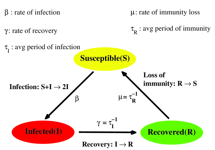
Details of stochastic simulation of epidemics on networks. We perform stochastic simulation of SIRS dynamics on the empirical and model contact networks using the Gillespie stochastic simulation algorithm Gillespie . There are three possible types of events that can occur in the network at any time: (i) A node (agent) that is in susceptible ($S$) state can undergo transition to infected ($I$) state. The propensity of a particular node in $S$ state to move to $I$ state is $\beta\,\frac{k_{inf}}{k}$, where $k_{inf}$ is the number of infected neighbors of the node while $k$ is the total number of its neighbors (i.e., degree). (ii) A node that is in $I$ state can undergo transition to recovered ($R$) state. Note that the process of an individual node recovering from infection is independent of its neighborhood. (iii) A node that is in $R$ state can undergo transition to $S$ state. The process of an individual node in $R$ state moving back to $S$ state is also independent of its neighborhood.

To simulate the stochastic time-evolution of an epidemic process in a network of $N$ nodes we need to determine (a) the sequence of time instants at which a transition event occurs and (b) the identity of the node at which the transition occurs. The latter determines the nature of the transition (viz., $S\rightarrow I$, $I\rightarrow R$ and $R\rightarrow S$), as this depends on the current state of the node ($S$, $I$ or $R$). The time-interval $\Delta{t}$ between two successive transition events is calculated as $\Delta{t}=-\log(\xi)/\Sigma^{N}_{i=1}p_{i}$, where $p_{i}$ are the rates associated with each of the $N$ transition events and $\xi\in[0,1]$ is a uniformly distributed random number in the unit interval. After this interval is obtained, we determine which one of the $N$ possible events will actually take place by generating another uniformly distributed random number $\zeta\in[0,\Sigma^{N}_{i=1}p_{i}]$ and pick the event $j$ that satisfies $\sum_{i=1}^{i=j-1}{p_{i}}<\zeta\leq\sum_{i=1}^{i=j}{p_{i}}$ ($j=1,\ldots,N$). This process is repeated until either (a) there are no infected individuals in the population such that the disease is declared extinct, or (b) the maximum time allowed for the simulation is reached.

Figure S2: The distribution of times for which an individual remains infected (top) and the period for which an individual is in the recovered state (bottom) in the stochastic model simulations. The different curves correspond to simulations performed with the rates of recovery ($\gamma$) and loss of immunity ($\mu$) kept constant (red) or time-varying (green and blue curves corresponding to model parameter $\beta=0.1$ and $1$ respectively). The distributions become more narrowly peaked about the respective mean values [viz., $\tau_{I}$ = 5 (top), $\tau_{R}=10$ (bottom)] with increasing values of $\beta$. Compared to the constant rate process (red curve), the probabilities of having extremely short or long periods of infection and recovery are markedly reduced for time-varying rates, especially as $\beta$ is increased. Note that $\beta=1$ for the stochastic simulation results shown in this paper.

Conventional stochastic simulations assume constant rates for all transition events which results in exponential distributions for the time periods during which an individual remains in the infected ($\tau_{I}$) or recovered ($\tau_{R}$) states. However, as the exponential distribution is peaked at the lower end of its support, this results in infected (recovered) individuals being most likely to recover (lose immunity) immediately after becoming infected (recovered), regardless of the mean infection (recovery) period for a disease. On the other hand, the long exponential tail of the distribution may result in some individuals remaining in the infected (recovered) period for durations extremely long relative to the mean period. For real diseases, on the other hand, individuals will likely remain infected (recovered) for about the same period - which implies that individual values of $\tau_{I}$ and $\tau_{R}$ will be relatively tightly clustered about the corresponding mean values Newman2010 .

In order to obtain distributions of $\tau_{I}$ and $\tau_{R}$ such that the individuals are relatively more homogeneous in terms of the infection and recovery periods (corresponding to reality) we have used transition rates from $I$ to $R$ ($\gamma$) and from $R$ to $S$ ($\mu$) that are time-varying. In particular, the rates are functions of the time duration for which an individual is in the infected or the recovered state (respectively), viz.,

$$\gamma_{i}=\exp{[\beta(\delta_{i}^{I}-\tau_{I})]},~{}~{}{\rm and},$$ (S1)

$$\mu_{i}=\exp{[\beta(\delta_{i}^{R}-\tau_{R})]},$$ (S2)

where $\delta_{i}^{I}$ ($\delta_{i}^{R}$) is the time elapsed from the instant an individual $i$ enters the infected (recovered) state and $\tau_{I},\tau_{R}$ are the average infection and recovery periods respectively. The tunable parameter $\beta$ determines how narrowly the resulting distribution of periods will be spread around the corresponding mean value. Fig. S2 compares the distributions of $\tau_{I}$ (top) and $\tau_{R}$ (bottom) obtained with a constant transition rate (‘null’), as well as two time-varying rate processes with different values of $\beta$. As can easily be seen, the distribution of the individual time periods become less dispersed with increasing $\beta$, so that events corresponding to very short or very long infection or recovery periods (compared to the mean values) become extremely unlikely. For all the stochastic simulation results shown here, we have chosen $\beta=1$. Small variations in the value of $\beta$ about this value do not change the results qualitatively. Furthermore, deterministic model simulations in which all individuals have the same $\tau_{I}$ and $\tau_{R}$ (corresponding to $\beta\rightarrow\infty$) also yield qualitatively similar results, implying that the model behavior is not sensitively dependent on the precise value of $\beta$ chosen as long as the distribution is relatively peaked narrowly about the mean.

Description of the simulation videos.

Figure S3: Snapshots from the simulation videos for the scenarios in which (top, Video 1) the disease dies out rapidly after the initial outbreak and (bottom, Video 2) the epidemic continues for as long as the simulation is continued. The large red circle indicates the individual that has become infected at the instant the snapshot is taken. Node colors represent different states, viz., blue: susceptible, red: infected and green: recovered.

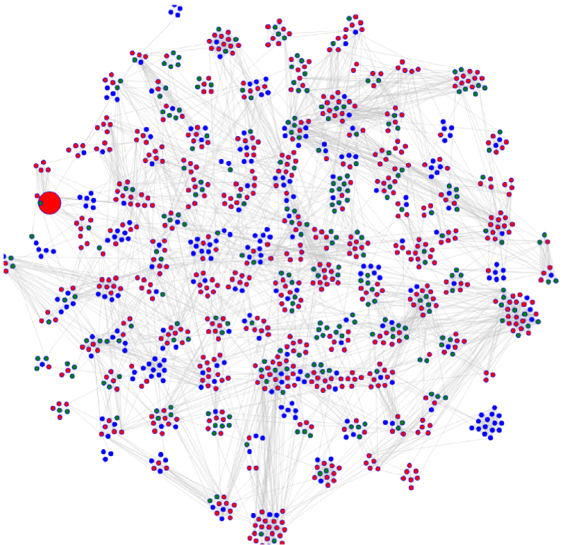
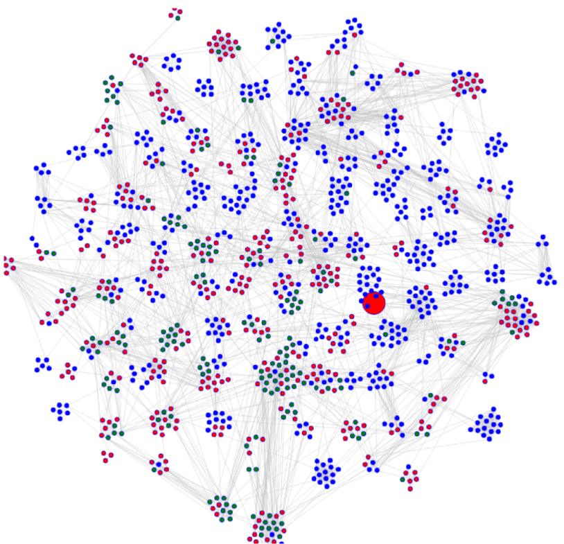
The two videos show simulated epidemics spreading in the social contact network of individuals in one of the villages in our database (Id. no. 55). The largest connected component of this network comprises 1151 nodes. The videos show two contrasting scenarios that one can observe for exactly the same choice of parameters. Video 1 corresponds to the situation when the infection dies out very early after initiation. Video 2 shows the scenario where the infection persists in the network upto the entire duration of the simulation. The three different states the nodes can be in are represented using three different colors, blue representing susceptible state, red infected state and green recovered state. Each individual event (i.e., a node becoming infected, recovered or susceptible) is shown with the node involved being highlighted. The “real time” elapsed between two consecutive events can be of any duration as this is a stochastic simulation.

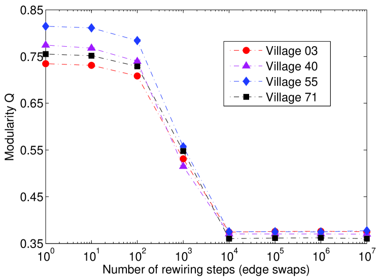
Details of randomization method for empirical networks. In order to understand the role of modularity in empirical social networks we need to compare them with an equivalent ‘randomized’ network having the same degree profile as the empirical network but which does not have modular organization. Such a randomized network ensemble can be constructed from the original network by a specific link swapping procedure described as follows. We choose any two modules of the original network (module 1 and module 2, say) and then from each, choose a pair of connected nodes (A,B from module 1 and C,D from module 2, say). The link exchange corresponds to removing the two intra-modular links and replacing them with two inter-modular links such that the degree of each node is preserved (e.g., removing the link between A & B and that between C & D, and connecting A to C and B to D). This process when repeated many times will result in a network whose modularity is much reduced compared to the empirical network, while preserving the original degree profile. This is shown in Fig. S4 which shows how the modular nature of a network, as measured by $Q$ Newman06 , changes as one randomizes empirical social networks by gradually increasing the number of rewiring steps. We observe that the modularity of the randomized network decreases rapidly when the number of link exchanges is increased beyond 100, but after about $10^{4}$ rewirings, $Q$ does not change appreciably. In our study, we have used $10^{6}$ link exchanges to generate randomized network ensembles.

Figure S4: The modular character of a degree-preserved randomized network, as measured by $Q$, decreases on increasing the number of random link exchanges starting from any one of four empirical social networks in our database (corresponding to villages whose Id numbers are shown in the legend). The four villages chosen for demonstration all exhibit a relatively high level of modular organization. In all four cases, the decrease in $Q$ saturates to an asymptotic value after around $10^{4}$ link exchange steps.

Effect of removing only inter-modular links from the empirical social networks.

Figure S5: Modular interconnectivity in the social network of a village (Id. no. 52) $N=1497$ individuals. (a) Matrix representing the average connection density between individuals belonging to the same network community and those belonging to different communities in the largest connected component of a village social network of southern India (contact data obtained from Ref. data1 ). The communities are defined in terms of connectivity within them being relatively denser in comparison to the overall connection density, and have been identified using a spectral algorithm Newman04 . The empirical network has been subsequently used to generate sparser contact networks by reducing the inter-modular connection density, keeping the connections within each module unchanged. (b) and (c) show the corresponding matrices for reduction by 50% and 90% respectively.

Comparing the progress of an epidemic on an empirical social network with community structure to that in the corresponding randomized network that is relatively homogeneous provides an important tool to evaluate the key role of modular organization in enhancing the persistence of epidemic processes on networks. However, apart from comparing the empirical networks having high modularity with corresponding randomized networks of relatively much lower modularity, one can also investigate networks having higher modularity that can be constructed from empirical social networks by selectively removing a fraction of the links that connect nodes belonging to different modules, while preserving all intra-modular links. An important limitation of this procedure is that it does not preserve the degree profile of the original network. Thus, the following results are indicative rather than conclusive.

Figure S6: The probability that persistence time of an epidemic exceeds a specified duration (viz., 5000 time units) in modular social networks (continuous curve) and the corresponding degree-preserved randomized networks (broken curves) as a function of the basic reproduction number of the epidemic for (a) 50% and (b) 90% reduction of the inter-modular connection density in the empirical contact network of a village in southern India.

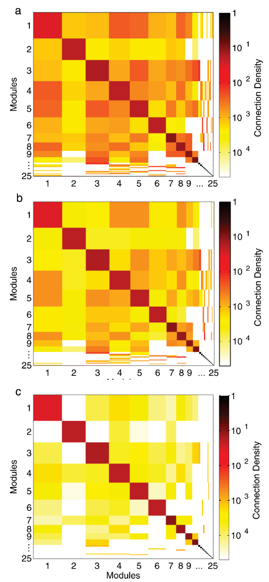
We show here that on increasing the modularity of the empirical network, persistence of the epidemic can be observed for higher values of $R_{0}$ compared to the original network. Fig. S5 (a) shows the empirical network matrix, representing the average connection density between individuals belonging to the same network community and those belonging to different communities. This empirical network was used to generate higher degree of modular organization of contact networks by reducing the inter-modular connection density by $50\%$ (b) and $90\%$ (c), keeping the connections within each module unchanged.

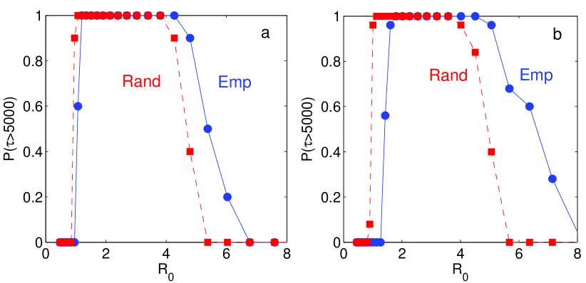
Fig. S6 (a-b) shows the probability that persistence time of an epidemic exceeds a specified duration (viz., 5000 time units) in the reduced inter-modular connection density by $50\%$ (a) and $90\%$ (b) empirical social network (blue continuous curve) and the corresponding degree-preserved randomized network (red broken curve) with the function of $R_{0}$. This result demonstrates that increased modularity in the network makes an epidemic persist for contagion having higher level of infectiousness (i.e., higher value of $R_{0}$).

Explaining persistence of epidemics in homogeneous networks.

Figure S7: Bifurcation diagram of the fraction of newly infected cases $x_{n}$ at each time step $n$ in a population of $N$ individuals under the homogeneous mean-field approximation such that the time-evolution of $x$ is described by $x(n+1)=[1-(1-\beta)^{k\sum_{j=0}^{\tau_{I}-1}x(n-j)}][1-\sum_{j=0}^{\tau_{I}+\tau_{R}-1}x(n-j)]$. The total infected fraction in the population at time $n$ is $f_{i}(n)=\sum_{j=0}^{\tau_{I}-1}x(n-j)$; if at any time $f_{i}$ falls below the threshold $1/N$ (i.e., not a single individual in the population is infected), indicated by the broken line, the disease becomes extinct. This is indeed seen to occur for $R_{0}\simeq 5.4$. For consistency with results shown in Fig. 2, we have chosen $N=1024$, $k=12$, $\tau_{I}=5$ and $\tau_{R}=10$. In the initial state $1\%$ of the population is infected after which the system is evolved for $10^{4}$ time steps for each value of $R_{0}$. In the diagram the final $10^{3}$ states in the time-evolution of $x$ are shown.

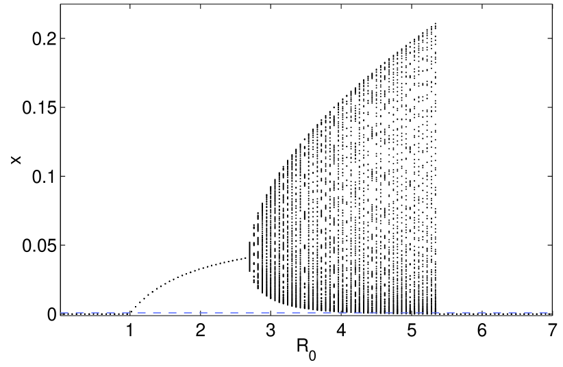
The persistence behavior of epidemics for an intermediate range of $R_{0}$ can be understood in the limit of a homogeneous network, as one can invoke a mean-field approximation that allows us to give an effective low-dimensional dynamical description of the system. We note that a disease having $R_{0}<1$ will not be able to initiate an epidemic regardless of the network structure, as the number of secondary infections arising through contact are actually less than the number of initially infected individuals. Thus, as the infected fraction of the population $f_{i}(=I/N)$ rapidly decays to zero, the time for which the disease persists in the population is typically short. For $R_{0}\geq 1$, relatively homogeneous networks (i.e., having higher values of $r$) show a rapid rise in the disease incidence characteristic of an epidemic as the network spreads the infection to a much larger fraction than that which had been infected initially. The infected fraction time-series then settles down to an irregular series of oscillations with the disease persisting in the population for the duration of simulation, provided $R_{0}$ is not too high. However, if $R_{0}$ is increased, we eventually observe a very different long-term behavior where the entire population becomes infected in a short space of time, followed by recovery and extinction of the disease. This can be explained in terms of a delay difference equation describing the time-evolution of infections under a mean-field approximation (where we can assume $k_{inf}=kf_{i}$). For such a case, the fraction of individuals that are infected at a particular time-step $n+1$ is $x_{n+1}=[1-(1-\beta)^{k\sum_{j=0}^{\tau_{I}-1}x(n-j)}][1-\sum_{j=0}^{\tau_{I}+\tau_{R}-1}x(n-j)]$. As can be seen from Fig. S7, the bifurcation diagram of the map shows that for an intermediate range of $R_{0}$ the epidemic will be persistent.

Construction procedure for model networks. The modular network model used in this paper follows from the definition of modularity and consists of $N$ nodes arranged into $M$ modules of different sizes. The size distribution of the modules has a Gaussian nature, whose dispersion can be tuned around an average value $n=N/M$, by changing the standard deviation $\sigma$. The connection probability between nodes in a module is $\rho_{i}$, and that between different modules is $\rho_{o}$. The parameter defining the model is the ratio of inter- to intra-modular connectivity, $\rho_{o}/\rho_{i}=r\in[0,1]$. For $r\rightarrow 0$, the network gets fragmented into isolated clusters, while as $r\rightarrow 1$, the network approaches a homogeneous random network. If $n_{i}$ is the size of module $i$ and $k$ is the average degree, the intra- and inter-modular connection densities can be expressed in terms of the different network parameters as $\rho_{i}=Nk/[\Sigma_{i}n_{i}(n_{i}-1)+\Sigma_{i}rn_{i}(N-n_{i})]$ and $\rho_{o}=r\rho_{i}$. The adjacency matrix for a contact network is constructed by randomly linking nodes within a module and between modules according to the above connection probabilities, respectively. Details will be provided in a forthcoming publication Menon15a .

Persistence of epidemics in modular network model.

Figure S8: Optimal modular organization of the contact network makes an infectious disease persistent. Space-time diagrams (top row) and the time-series (bottom row) of the infected fraction $f_{i}$ of population shown for contact networks having (a) $r=2\times 10^{-4}$, (b) $r=2\times 10^{-3}$ and (c) $r=2\times 10^{-2}$, for a disease with $R_{0}=6$. While both for the case of almost isolated modules (a) and the relatively homogeneous network (c), the epidemic becomes extinct within 100 time units, for an intermediate value of modularity organization (b) the epidemic persists for as long as the simulation is continued. For all simulation results shown here we have used a network of $N=1024$ nodes having $M=64$ modules of size $n=16$ each. The nodes have average degree $k=12$, with $\tau_{I}=5$ and $\tau_{R}=10$ time units.

Figure S9: (a) The distribution of the time $\tau$ (with logarithmic binning) for which an epidemic with $R_{0}=6$ persists in the network shows a bimodal nature for higher values of the modularity parameter $r$, with the upper branch diverging as the network becomes more modular. For lower values of $r$, the distribution is unimodal and the average value of $\tau$ decreases rapidly as the modules become effectively isolated. Results shown for $N=1024$ with $M=64$ modules, each with $n=16$ nodes having an average degree $k=12$. (b) The probability that the epidemic persists for more than $10^{4}$ time units is shown as function of the modularity parameter $r$ for networks having different number of modules $M$ ($N=1024$ with each node having average degree $k=12$.)

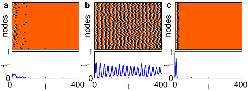
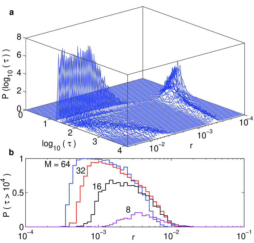
As already described in the main text, an epidemic that becomes extinct within a short time interval in a homogeneous network ($r\sim 1$), can become recurrent when the network is optimally modular, persisting in the system for extremely long times. However, as one approaches the limit of the modules becoming almost isolated ($r\sim 0$), the infection is unable to transfer from one module to another and the epidemic again becomes extinct rapidly. This is shown explicitly in Fig. S8.

Fig. S9 (a) shows the variation of the probability distribution of persistence time $\tau$ with network modularity. The distribution of $\tau$ over the range of $r$ for which the epidemic persists indefinitely shows a bimodal nature. The lower branch corresponds to the time-scale over which the disease lasts in a single module, and as can be seen the peak of the distribution remains almost unchanged as $r$ is varied. For low $r$, it represents the realizations in which the disease fails to break out of the module(s) in which the initial outbreak occurs. For high $r$, the contagion spreads rapidly through the system, lasting almost as long in the entire system as it does in any given module. The upper branch, on the other hand, corresponds to the realizations where the epidemic propagation between modules is slowed down by the modular organization. Note that the peak of this branch diverges in the optimal range of $r$ where the epidemic becomes persistent in the network. Moreover, the bulk of the distribution moves from the lower to the upper branch in this parameter range. Fig. S9 (b) shows that while the optimal modularity range is not overly dependent on the number of modules $M$ in the network, the persistence effect does become more prominent as one increases $M$, while keeping the total size of the network ($N$) invariant. We also observe that the value of $r$ at which the peak of the persistence behavior occurs reduces with increasing $M$.

Table S1: Summary details of the contact network properties for the villages considered in this study.

SlNo	Nodes	LCC	$<k>$	Modules	Q	$\mu_{sz}$	$\sigma_{sz}$	LMS	r
1	843	825	8.2	24	0.6782	34.375	19.6783	72	0.02
2	877	810	7.2123	23	0.7396	35.2174	22.446	91	0.0149
3	1380	1318	7.9841	25	0.7312	52.72	38.6539	189	0.0161
4	1025	957	7.2403	25	0.7315	38.28	25.6117	99	0.0155
5	650	641	7.869	25	0.7477	25.64	20.268	70	0.0154
6	451	434	6.9954	24	0.7036	18.0833	15.4809	63	0.0193
7	732	719	9.0668	23	0.7078	31.2609	25.1555	83	0.0195
8	444	440	8.2818	22	0.7051	20.0	20.3693	75	0.0222
9	928	914	8.4497	22	0.703	41.5455	33.3517	141	0.0212
10	354	346	8.8353	19	0.6614	18.2105	15.2784	48	0.0294
11	605	589	7.8727	23	0.6986	25.6087	23.814	92	0.023
12	794	760	7.7132	23	0.7225	33.0435	20.0531	74	0.0167
13	-	-	-	-	-	-	-	-	-
14	675	645	8.1054	23	0.7453	28.0435	21.1115	91	0.0155
15	853	852	8.9648	23	0.6954	37.0435	24.5985	90	0.0204
16	712	693	9.3059	22	0.7152	31.5	24.7694	99	0.0201
17	879	850	8.6494	25	0.7284	34.0	28.1539	123	0.0177
18	1146	1140	9.157	24	0.7522	47.5	34.87	127	0.0149
19	1134	1118	9.2844	24	0.7484	46.5833	31.0979	131	0.014
20	714	633	8.6477	23	0.744	27.5217	18.5117	66	0.0139
21	1046	1011	8.6311	25	0.7347	40.44	32.0063	116	0.0164
22	-	-	-	-	-	-	-	-	-
23	1252	1186	8.6636	24	0.7572	49.4167	37.5732	125	0.0144
24	835	820	9.3098	25	0.7222	32.8	22.735	79	0.0165
25	1313	1286	9.4619	25	0.7751	51.44	32.2404	124	0.0116
26	674	666	9.0405	21	0.7576	31.7143	28.3198	127	0.0152
27	708	682	7.4091	25	0.7408	27.28	18.3794	67	0.0144
28	1612	1570	9.5822	25	0.7812	62.8	39.8628	163	0.0112
29	1337	1270	7.8276	25	0.7651	50.8	26.9741	115	0.0113
30	689	675	8.8607	23	0.7489	29.3478	25.1441	91	0.0165
31	851	819	9.0317	25	0.7893	32.76	22.0023	97	0.0106
32	1181	1136	9.6514	25	0.7296	45.44	30.0281	102	0.0157
33	843	824	7.7415	25	0.7279	32.96	29.0799	101	0.0174
34	692	628	7.1385	24	0.7702	26.1667	26.1465	115	0.0128
35	806	756	7.2302	25	0.758	30.24	27.388	106	0.0133
36	1214	1168	8.8733	24	0.7147	48.6667	53.5698	197	0.0214
37	500	482	7.7759	16	0.6593	30.125	24.2922	91	0.0324
38	736	726	8.1267	24	0.7723	30.25	21.9037	82	0.0124
39	1339	1294	9.1376	25	0.7666	51.76	31.9466	134	0.012
40	1097	1064	8.0442	25	0.7713	42.56	42.0562	168	0.0135
41	724	703	7.8862	20	0.7163	35.15	26.3615	76	0.0203
42	853	805	8.0807	25	0.7587	32.2	32.3394	117	0.0153
43	875	861	8.295	24	0.7331	35.875	30.5195	121	0.016
44	978	965	8.8518	25	0.7212	38.6	40.4366	136	0.0202
45	1073	1044	8.2356	25	0.7782	41.76	29.4405	113	0.0116
46	1257	1216	7.8544	24	0.7683	50.6667	34.6671	155	0.0125
47	680	660	8.5848	24	0.719	27.5	20.4185	70	0.0174
48	808	794	8.9232	24	0.6998	33.0833	31.5686	116	0.0225
49	766	689	8.7083	22	0.6439	31.3182	35.6987	140	0.0362
50	999	937	8.9883	25	0.6994	37.48	43.5175	145	0.0235
51	1061	1015	10.6591	21	0.6734	48.3333	55.2943	187	0.0308
52	1525	1497	10.4369	25	0.7339	59.88	69.595	276	0.0192
53	642	630	9.0683	23	0.6573	27.3913	32.5746	110	0.0322
54	467	458	10.1528	20	0.6636	22.9	28.0141	111	0.0326
55	1180	1151	7.9644	24	0.8192	47.9583	33.5478	127	0.0087
56	573	553	7.8807	23	0.7223	24.0435	20.6955	76	0.0189
57	948	919	8.2459	25	0.7222	36.76	29.2278	130	0.0174
58	914	905	8.8541	25	0.744	36.2	27.0289	110	0.0153
59	1599	1552	8.5393	24	0.7936	64.6667	46.4091	182	0.0108
60	1775	1729	8.7953	25	0.789	69.16	42.0692	215	0.0105
61	591	572	9.3776	20	0.7299	28.6	25.4213	104	0.0191
62	994	980	9.1816	24	0.7676	40.8333	30.4872	131	0.013
63	786	774	8.0284	23	0.7833	33.6522	23.392	91	0.0119
64	1286	1265	8.7763	25	0.7926	50.6	32.3988	115	0.0103
65	1331	1301	9.3766	24	0.7101	54.2083	42.7444	149	0.0194
66	814	790	7.8848	23	0.7353	34.3478	29.078	102	0.0173
67	893	885	8.5401	22	0.7311	40.2273	36.4778	128	0.0192
68	663	655	8.1389	22	0.7014	29.7727	26.6218	90	0.0225
69	875	866	10.4688	23	0.6739	37.6522	42.5457	148	0.0281
70	899	891	9.3547	20	0.6634	44.55	37.4639	129	0.028
71	1387	1345	8.3836	24	0.7556	56.0417	44.8046	151	0.0144
72	999	977	8.6192	25	0.6973	39.08	33.5511	147	0.0217
73	870	858	9.4767	22	0.7207	39.0	31.7905	101	0.0199
74	743	724	8.2735	23	0.7707	31.4783	22.9307	89	0.0131
75	831	815	10.0454	24	0.7199	33.9583	43.6305	170	0.0236
76	1154	1126	8.3064	25	0.7878	45.04	34.5861	128	0.0114
77	707	671	8.2355	22	0.7551	30.5	24.5352	82	0.015

References

- (1) The World Health Report 2004 (World Health Organization, Geneva, 2004).
- (2) D. M. Morens, G. K. Folkers and A. S. Fauci, Nature (Lond.) 430, 242 (2004).
- (3) A. S. Fauci, N. A. Touchette and G. K. Folkers, Emerg. Infect. Dis. 11, 519 (2005).
- (4) K. T. Jones et al., Nature (Lond.) 451, 990 (2008).
- (5) S. S. Morse et al., Lancet, 380, 1956 (2012).
- (6) A. Dobson and J. Foufopoulos, Phil. Trans. Roy. Soc. B, 356, 1001 (2001).
- (7) R. S. Kovats, M. J. Bouma, S. Hajat, E. Worrall and A. Haines, Lancet 362, 1481 (2003).
- (8) B. Sultan, K. Labadi, J.-F. Guégan and S. Janicot, PLoS Medicine 2, e6 (2005).
- (9) M. Kitsak, L. K. Gallos, S. Havlin, F. Liljeros, L. Muchnik, H. E. Stanley, and H. A. Makse, Nature Phys. 6, 888 (2010).
- (10) A. V. Goltsev, S. N. Dorogovtsev, J. G. Oliveira and J. F. F. Mendes, Phys. Rev. Lett. 109, 128702 (2012).
- (11) R. Pastor-Satorras, C. Castellano, P. Van Mieghem and A. Vespignani, Rev. Mod. Phys. 87, 925 (2015).
- (12) G. Schehr and S. N. Majumdar, Phys. Rev. Lett. 99, 060603 (2007).
- (13) S. N. Majumdar, A. Rosso and A. Zoia, Phys. Rev. Lett. 104, 020602 (2010).
- (14) A. J. Bray, S. N. Majumdar and G. Schehr, Adv. Phys. 62, 225 (2013).
- (15) S. Wasserman, Social Network Analysis (Cambridge University Press, Cambridge, 1994).
- (16) M. Girvan and M. E. J. Newman, Proc. Natl. Acad. Sci. U.S.A. 99, 7821 (2002).
- (17) J.-P. Onnela, J. Saramaki, J. Hyvonen, G. Szabo, D. Lazer, K. Kaski, J. Kertesz and A.-L. Barabasi, Proc. Natl. Acad. Sci. U.S.A. 104, 7332 (2007).
- (18) A. Nematzadeh, E. Ferrara, A. Flammini and Y.-Y. Ahn, Phys. Rev. Lett. 113, 088701 (2014).
- (19) Z. Liu and B. Hu, EPL 72, 315 (2005).
- (20) L. Huang, K. Park and Y.-C. Lai, Phys. Rev. E 73, 035103(R) (2006)
- (21) W. Huang and C. Li, J. Stat. Mech., P01014 (2007).
- (22) H. Zhao and Z. Y. Gao, EPL 79, 38002 (2007).
- (23) R. H. Griffin and C. L. Nunn, Evol. Ecol. 26, 779 (2012).
- (24) N. Masuda, New J. Phys. 11, 123018 (2009).
- (25) M. Salathé and J. H. Jones, PLoS Comput Biol 6, e1000736 (2010).
- (26) D. J. D. Earn, P. Rohani and B. T. Grenfell, Proc. R. Soc. B 265, 7 (1998).
- (27) M. S. Bartlett, J. Roy. Stat. Soc. Ser. A 120, 48 (1957).
- (28) R. M. Anderson and R. M. May, Infectious Diseases of Humans: Dynamics and Control (Oxford University Press, Oxford, 1991).
- (29) M. J. Keeling and B. T. Grenfell, J. Theor. Biol. 203, 51 (2000).
- (30) D. T. Gillespie, J. Phys. Chem. 81, 2340 (1977).
- (31) M. J. Keeling and B. T. Grenfell, Science 275, 65 (1997).
- (32) A. Lloyd, Theor. Popn. Biol. 60, 59 (2001).
- (33) A. Banerjee, A. G. Chandrasekhar, E. Duflo and M. O. Jackson, Science 341, 1236498 (2013).
- (34) J. Reichardt and S. Bornholdt, Phys. Rev. E 74, 016110 (2006).
- (35) See supplementary material.
- (36) M. E. J. Newman, Proc. Natl. Acad. Sci. USA 103, 8577 (2006).
- (37) J. Lin, IEEE T. Inform. Theory 37, 145 (1991).
- (38) R. K. Pan and S. Sinha, EPL 85, 68006 (2009).
- (39) A. Pathak, S. N. Menon and S. Sinha, in preparation.
SUPPLEMENTARY MATERIAL
- (1) https://dataverse.harvard.edu/dataset.xhtml?persistentId=hdl:1902.1/21538
- (2) A. Banerjee, A. G. Chandrasekhar, E. Duflo, M. O. Jackson, Science 341, 1236498 (2013).
- (3) J. Reichardt and S. Bornholdt, Phys. Rev. E 74, 016110 (2006).
- (4) C. H. Wirsig von König, S. Postels-Multani, H. L. Bock and H. J. Schmitt, Lancet 346, 1326 (1995).
- (5) N. C. Grassly, C. Fraser and G. P. Garnett, Nature (Lond.) 433, 417 (2005).
- (6) C. M. Pease, Theor. Popn. Biol. 31, 422 (1987).
- (7) A. J. Hay, V. Gregory, A. R. Douglas and Y. P. Lin, Philos. Trans. R. Soc. Lond. B 356 ,1861 (2001).
- (8) M. B. Hooten, J. Anderson and L. A. Waller, Spatiotemporal Epidemiol. 1, 177 (2010).
- (9) H. W. Hethcote, Math. Biosci. 28, 335 (1976).
- (10) D. T. Gillespie, J. Phys. Chem. 81, 2340 (1977).
- (11) M. E. J. Newman, Networks: An Introduction (Oxford University Press, Oxford, 2010).
- (12) M. E. J. Newman, Proc. Natl. Acad. Sci. USA 103, 8577 (2006).
- (13) M. E. J. Newman, Phys. Rev. E 69, 066133 (2004).
- (14) A. Pathak, S. N. Menon and S. Sinha, in preparation.