Topological susceptibility in finite temperature (2+1)-flavor QCD using gradient flow

Abstract

We compute the topological charge and its susceptibility in finite temperature (2+1)-flavor QCD on the lattice applying a gradient flow method. With the Iwasaki gauge action and nonperturbatively $O(a)$-improved Wilson quarks, we perform simulations on a fine lattice with $a\simeq 0.07\,\mathrm{fm}$ at a heavy $u$, $d$ quark mass with $m_{\pi}/m_{\rho}\simeq 0.63$ but approximately physical $s$ quark mass with $m_{\eta_{ss}}/m_{\phi}\simeq 0.74$. In a temperature range from $T\simeq 174\,\mathrm{MeV}$ ($N_{t}=16$) to $697\,\mathrm{MeV}$ ($N_{t}=4$), we study two topics on the topological susceptibility. One is a comparison of gluonic and fermionic definitions of the topological susceptibility. Because the two definitions are related by chiral Ward-Takahashi identities, their equivalence is not trivial for lattice quarks which violate the chiral symmetry explicitly at finite lattice spacings. The gradient flow method enables us to compute them without being bothered by the chiral violation. We find a good agreement between the two definitions with Wilson quarks. The other is a comparison with a prediction of the dilute instanton gas approximation, which is relevant in a study of axions as a candidate of the dark matter in the evolution of the Universe. We find that the topological susceptibility shows a decrease in $T$ which is consistent with the predicted $\chi_{\mathrm{t}}(T)\propto(T/T_{\mathrm{pc}})^{-8}$ for three-flavor QCD even at low temperature $T_{\mathrm{pc}}<T\mathrel{\hbox to0.0pt{\raise 2.20013pt\hbox{$<$}\hss}{\lower 2.20013pt\hbox{$\sim$}}}1.5\,T_{\mathrm{pc}}$.

I Introduction

The axion is introduced into QCD to solve the strong CP problem through the Peccei-Quinn mechanism Peccei:1977hh . Simultaneously, the axion is a candidate of the cold dark matter where the temperature dependence of its mass plays an important role in the estimation of its cosmic abundance Preskill ; Abbott ; Dine . The axion mass squared is proportional to the topological susceptibility $\chi_{\mathrm{t}}$. The temperature dependence of $\chi_{\mathrm{t}}$ is predicted by the dilute instanton gas approximation (DIGA) tHooft:1976snw to be $\chi_{\mathrm{t}}(T)\propto(T/T_{\mathrm{pc}})^{-8}$ in a high temperature limit for three flavors Gross:1980br , where $T_{\mathrm{pc}}$ is the pseudocritical temperature. Recently, $\chi_{\mathrm{t}}(T)$ is studied in lattice QCD in the quenched approximation Berkowitz:2015aua ; Kitano:2015fla ; Borsanyi:2015cka and with (2+1)-flavors Bonati:2015vqz ; Petreczky:2016vrs or (2+1+1)-flavors Borsanyi:2016ksw of staggered quarks. In Ref. Bonati:2015vqz , the decreasing behavior is found to be much slower than DIGA, while in Ref. Petreczky:2016vrs , the power is found to be consistent with DIGA above $1.5\,T_{\mathrm{pc}}$ but is a bit more moderate for $T_{\mathrm{pc}}<T\mathrel{\hbox to0.0pt{\raise 2.20013pt\hbox{$<$}\hss}{\lower 2.20013pt\hbox{$\sim$}}}1.5\,T_{\mathrm{pc}}$. In this paper, we study this issue in $N_{f}=$2+1 lattice QCD with improved Wilson quark action based on the gradient flow Narayanan:2006rf ; Luscher:2009eq ; Luscher:2010iy ; Luscher:2011bx ; Luscher:2013cpa ; reviewLattice and calculate the temperature dependence of topological charge and its susceptibility in the range $T\simeq 174$-$697\,\mathrm{MeV}\simeq(0.92\mathrm{-}3.67)T_{\mathrm{pc}}$.

A problem in the calculation of topological charge on the lattice is the UV singularities in composite operators, which becomes acute when chiral symmetry is broken explicitly. In particular, $\chi_{\mathrm{t}}$ defined in terms of gauge fields (“gluonic definition”) and that in terms of quark fields (“fermionic definition”), which are equivalent in the continuum theory or with Ginsparg-Wilson lattice quarks Giusti:2004qd , are largely discrepant with more conventional nonchiral lattice quarks. For example, a recent study with improved staggered quarks reports more than 100 times larger gluonic $\chi_{\mathrm{t}}$ than fermionic one at $T\sim 1.5\,T_{\mathrm{pc}}$ on finite lattices Petreczky:2016vrs . Much efforts have been dedicated to avoid the singular behavior Luscher:2004fu ; Giusti:2008vb ; Luscher:2010ik . We solve the above problem by making use of a UV divergence-free property of the gradient flow Narayanan:2006rf ; Luscher:2009eq ; Luscher:2010iy ; Luscher:2011bx ; Luscher:2013cpa . This is an extension of our previous study on energy-momentum tensor and chiral condensate ourEOSpaper using the method of Refs. Suzuki:2013gza ; Makino:2014taa ; Hieda:2016lly .

The gradient flow we adopt is described in Ref. ourEOSpaper . The gauge field is flowed with fictitious time $t$ as Luscher:2010iy

$$\partial_{t}B_{\mu}(t,x)=D_{\nu}G_{\nu\mu}(t,x),\quad B_{\mu}(t=0,x)=A_{\mu}(x),$$ (1)

where

$$G_{\mu\nu}\equiv\partial_{\mu}B_{\nu}-\partial_{\nu}B_{\mu}+[B_{\mu},B_{\nu}],$$ (2)

$$D_{\nu}G_{\nu\mu}\equiv\partial_{\nu}G_{\nu\mu}+[B_{\nu},G_{\nu\mu}].$$ (3)

The gradient flow for quark fields is given by Luscher:2013cpa

$$\partial_{t}\chi_{f}(t,x)=\Delta\chi_{f}(t,x),\quad\chi_{f}(t=0,x)=\psi_{f}(x),$$ (4)

$$\partial_{t}\bar{\chi}_{f}(t,x)=\bar{\chi}_{f}(t,x)\overleftarrow{\Delta},\quad\bar{\chi}_{f}(t=0,x)=\bar{\psi}_{f}(x),$$ (5)

where $f=u$, $d$ and $s$, with

$$\Delta\chi_{f}\equiv D_{\mu}D_{\mu}\chi_{f},\quad D_{\mu}\chi_{f}\equiv\left[\partial_{\mu}+B_{\mu}\right]\chi_{f},$$ (6)

$$\bar{\chi}_{f}\overleftarrow{\Delta}\equiv\bar{\chi}_{f}\overleftarrow{D}_{\mu}\overleftarrow{D}_{\mu},\quad\bar{\chi}_{f}\overleftarrow{D}_{\mu}\equiv\bar{\chi}_{f}\left[\overleftarrow{\partial}_{\mu}-B_{\mu}\right].$$ (7)

The flowed fields can be viewed as smeared fields over a range of about $\sqrt{8t}$ in four dimensions. Operators constructed with the flowed fields are shown to be free from UV divergence when multiplied with an appropriate wave function renormalization factor to the quark fields Luscher:2011bx ; Luscher:2013cpa . We can thus consider the flowed operators as renormalized operators in a new renormalization scheme with the scale $\sqrt{8t}$.

II Simulation parameters

Measurements are performed on $N_{f}=2+1$ QCD configurations generated for Refs. Ishikawa:2007nn ; Umeda:2012er adopting a nonperturbatively $O(a)$-improved Wilson quark action and the renormalization group-improved Iwasaki gauge action Iwasaki:2011np . Our gauge coupling constant $\beta=2.05$ corresponds to the lattice spacing $a=0.0701(29)\,\mathrm{fm}$ ($1/a\simeq 2.79\,\mathrm{GeV}$). The hopping parameters $\kappa_{u}=\kappa_{d}\equiv\kappa_{ud}=0.1356$ and $\kappa_{s}=0.1351$ correspond to heavy $u$ and $d$ quarks, $m_{\pi}/m_{\rho}\simeq 0.63$, and almost physical $s$ quark, $m_{\eta_{ss}}/m_{\phi}\simeq 0.74$. The bare PCAC quark masses are $a\,m_{ud}=0.02105(17)$ and $a\,m_{s}=0.03524(26)$. With the fixed-scale approach Levkova:2006gn ; Umeda:2008bd , the temperature $T=1/(aN_{t})$ is varied by changing the temporal lattice size $N_{t}$. We adopt $N_{t}=16$, 14, 12, 10, 8, 6, and 4, which correspond to $T\simeq 174$, 199, 232, 279, 348, and 697 MeV, respectively ($T/T_{\mathrm{pc}}\simeq 0.92$, 1.05, 1.22, $\cdots$ 3.67, assuming the pseudocritical temperature of $T_{\mathrm{pc}}\sim 190$ MeV Umeda:2012er ). See Table 1 for temperature and number of configurations at each $N_{t}$. Spatial box size is $N_{s}^{3}=32^{3}$ for finite temperature and $28^{3}$ for zero temperature. To avoid unphysical effects due to overlapped smearing, we require

$$t\leq t_{1/2}\equiv\frac{1}{8}\left[\min\left(N_{t}/2,N_{s}/2\right)\right]^{2}.$$ (8)

Our study of the energy-momentum tensor and chiral condensate on these configurations suggests that our lattices are sufficiently fine but the lattices with $N_{t}\mathrel{\hbox to0.0pt{\raise 2.20013pt\hbox{$<$}\hss}{\lower 2.20013pt\hbox{$\sim$}}}8$ suffer from small-$N_{t}$ lattice artifacts ourEOSpaper .

The differential equations for the gradient flow are solved by the third-order Runge-Kutta method Luscher:2010iy ; Luscher:2013cpa with the step size of $\epsilon=0.02$. Quark observables are evaluated with the noisy estimator method ourEOSpaper . The number of noise vectors is 20 for each color. The statistical errors are estimated by a jackknife analysis with bin size of 300 in Monte Carlo time as determined from the autocorrelation.

$T$ (MeV)	$T/T_{\mathrm{pc}}$	$N_{t}$	$t_{1/2}$	Number of confs.
$0$	$0$	$56$	$24.5$	$650$
$174$	$0.92$	$16$	$8$	$1440$
$199$	$1.05$	$14$	$6.125$	$1270$
$232$	$1.22$	$12$	$4.5$	$1290$
$279$	$1.47$	$10$	$3.125$	$780$
$348$	$1.83$	$8$	$2$	$510$
$464$	$2.44$	$6$	$1.125$	$500$
$697$	$3.67$	$4$	$0.5$	$700$

Table 1: Parameters for the numerical simulation: Temperature in MeV, $T/T_{\mathrm{pc}}$ assuming $T_{\mathrm{pc}}=190$ MeV, $N_{t}$, $t_{1/2}$, and number of configurations. Configurations are stored every five trajectories ($\tau=5$) at finite temperature and every $10$ trajectories at zero temperature. The bare coupling and the hopping parameter is set to $\beta=2.05$, $\kappa_{ud}=0.1356$, and $\kappa_{s}=0.1351$ for every $N_{t}$. Spatial box size is $32^{3}$ for $T>0$ and $28^{3}$ for $T=0$.

III Gluonic definition

The most popular definition of the topological charge is to use the gauge field strength $F\tilde{F}$ accompanied with a cooling step GarciaPerez:1998ru ; Bonati:2014tqa ; Namekawa:2015wua ; Alexandrou:2015yba . The gradient flow provides us with a cooling procedure Bonati:2014tqa and a renormalization procedure simultaneously. Let us define the topological charge density by the flowed gauge field as Luscher:2010iy

$$q(t,x)=\frac{1}{64\pi^{2}}\epsilon_{\mu\nu\rho\sigma}G_{\mu\nu}^{a}(t,x)G_{\rho\sigma}^{a}(t,x),\quad\epsilon_{0123}=1,$$ (9)

and the topological charge as $Q(t)=\int d^{4}x\,q(t,x)$. There are several alternative choices of lattice operators for the quadratic term of the field strength tensor $G_{\mu\nu}$. In this study, we adopt the tree-level $O(a^{4})$-improved field strength squared by combing the clover operator with four plaquette Wilson loops and that with four $1\times 2$ rectangle Wilson loops AliKhan:2001ym . The normalization of the topological charge thus defined is shown to be consistent with the Ward-Takahashi (WT) relation associated with the flavor singlet chiral symmetry Ce:2015qha ; Hieda:2016lly and the operator $Q(t)$ is independent of the flow time in the continuum limit Luscher-talk ; Ce:2015qha .

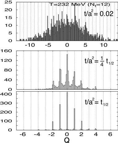
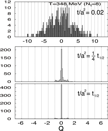
Figure 1: Histogram of the topological charge with the gluonic definition at $T\simeq 232$ MeV (left panel) and $T\simeq 348$ MeV (right panel). The upper, middle, and lower plots in each panel are for flow times $t/a^{2}=0.02$, $\frac{1}{4}t_{1/2}$, and $t_{1/2}$, respectively.

In the left panel of Fig. 1, we plot the histogram of $Q$ with the gluonic definition at $T\simeq 232$ MeV, obtained at various flow times. We see that $Q$ accumulates to integer values as we flow the gauge configuration, i.e., the gradient flow works well as a renormalization with canonical normalization. We find that $Q$ has well wide distribution on nonzero values at $T\mathrel{\hbox to0.0pt{\raise 2.20013pt\hbox{$<$}\hss}{\lower 2.20013pt\hbox{$\sim$}}}279$ MeV ($N_{t}\mathrel{\hbox to0.0pt{\raise 2.20013pt\hbox{$>$}\hss}{\lower 2.20013pt\hbox{$\sim$}}}10$) but starts to freeze at $Q=0$ at $T\mathrel{\hbox to0.0pt{\raise 2.20013pt\hbox{$>$}\hss}{\lower 2.20013pt\hbox{$\sim$}}}348$ MeV ($N_{t}\mathrel{\hbox to0.0pt{\raise 2.20013pt\hbox{$<$}\hss}{\lower 2.20013pt\hbox{$\sim$}}}8$), as shown in the right panel of Fig. 1.

Figure 2: The $\chi_{\mathrm{t}}(t,a)$ with the gluonic definition as a function of the flow time $t/a^{2}$. From the top left: $T\simeq 0$, $174$, $199$, $232$, $279$, $348$, $464$, and $697$ MeV, respectively. Vertical axis is in lattice unit. The vertical dotted lines for the higher three temperatures indicate $t_{1/2}$. For the lower five temperatures, $t_{1/2}$ resides at the highest $t$ in the figure.

The topological susceptibility with the gluonic definition is defined by

$$\chi_{\mathrm{t}}=\frac{1}{V_{4}}\left(\left\langle Q^{2}\right\rangle-\left\langle Q\right\rangle^{2}\right).$$ (10)

In Fig. 2 we show the results of $\chi_{\mathrm{t}}(t,a)$ as a function of the flow time. At $T\mathrel{\hbox to0.0pt{\raise 2.20013pt\hbox{$<$}\hss}{\lower 2.20013pt\hbox{$\sim$}}}279$ MeV, we find wide plateaus below $t_{1/2}$ reflecting the flow time invariant property in the continuum Luscher-talk ; Ce:2015qha . On the other hand, at $T\mathrel{\hbox to0.0pt{\raise 2.20013pt\hbox{$>$}\hss}{\lower 2.20013pt\hbox{$\sim$}}}348$ MeV, $\chi_{\mathrm{t}}(t,a)$ does not show a plateau up to $t_{1/2}$. On these lattices, we cannot extract a physical value due to lattice artifacts. We thus concentrate on the range $T\mathrel{\hbox to0.0pt{\raise 2.20013pt\hbox{$<$}\hss}{\lower 2.20013pt\hbox{$\sim$}}}279$ MeV. We also test other operators for the quadratic term of $G_{\mu\nu}$, including the clover operator only with plaquettes, that with only rectangle loops, and square of the imaginary part of the plaquette. We find that the results are consistent with each other within statistical errors. The results of the topological susceptibility with the gluonic definition are summarized later.

IV Fermionic definition

In the continuum QCD, the topological susceptibility is related to the disconnected two point function of the flavor-singlet pseudoscalar through chiral WT identities Bochicchio:1984hi ; Giusti:2004qd ,

$$\left\langle\partial_{\mu}A_{\mu}^{a}(x)\,{\cal O}\right\rangle-2m\left\langle\pi^{a}(x)\,{\cal O}\right\rangle+2n_{f}\delta^{a0}\left\langle q(x)\,{\cal O}\right\rangle=i\left\langle\delta^{a}{\cal O}\right\rangle,$$ (11)

where $n_{f}$ is the number of degenerate flavors with mass $m$ ($n_{f}=2$ and $m=m_{ud}$ in our case) and $A_{\mu}^{a}(x)=\bar{\psi}(x)T^{a}\gamma_{\mu}\gamma_{5}\psi(x)$, $\pi^{a}(x)=\bar{\psi}(x)T^{a}\gamma_{5}\psi(x)$ in which $T^{a}$ is the generator in the degenerate flavor space and $\psi$ is the multiplet of the degenerate flavors. We set $T^{0}=1$ (i.e., $a=0$ stands for singlet) and ${\rm tr}\left(T^{a}T^{b}\right)=\delta^{ab}$ for $a,b\geq 1$.

The desired relation is derived as follows: From singlet WT identities for ${\cal O}=Q$ and ${\cal O}=P^{0}$,

$$-m\left\langle P^{0}Q\right\rangle+n_{f}\left\langle Q^{2}\right\rangle=0,$$ (12)

$$-m\left\langle P^{0}P^{0}\right\rangle+n_{f}\left\langle Q\,P^{0}\right\rangle=-\left\langle S^{0}\right\rangle,$$ (13)

where $P^{a}\equiv\int d^{4}x\,\pi^{a}(x)$ and $S^{a}\equiv\int d^{4}x\,\bar{\psi}(x)T^{a}\psi(x)$, we obtain

$$n_{f}^{2}\left\langle Q^{2}\right\rangle=m^{2}\left\langle P^{0}P^{0}\right\rangle-m\left\langle S^{0}\right\rangle.$$ (14)

On the other hand, for nonsinglet ${\cal O}=P^{b}$,

$$-2m\left\langle P^{a}P^{b}\right\rangle=-\left(\delta^{ab}\frac{2}{n_{f}}\left\langle S^{0}\right\rangle+d_{abc}\left\langle S^{c}\right\rangle\right),$$ (15)

where $a,b,c\geq 1$. Since the nonsinglet flavor symmetry is not broken we get

$$\chi_{\mathrm{t}}=\frac{1}{V_{4}}\left\langle Q^{2}\right\rangle=\frac{m^{2}}{V_{4}n_{f}^{2}}\left(\left\langle P^{0}P^{0}\right\rangle-n_{f}\left\langle P^{a}P^{a}\right\rangle\right),$$ (16)

where the sum is not taken over $a$ in the right-hand side. The right-hand side is nothing but the disconnected part of the singlet pseudoscalar two point function. The right-hand side of (16) may have power divergences with Wilson or staggered fermions since the chiral symmetry is broken explicitly Giusti:2004qd ; Luscher:2004fu .

To overcome the difficulties in the calculation of renormalized fermion bilinear operators due to violation of symmetries on the lattice, we adopt the method of Ref. Hieda:2016lly based on a small-$t$ expansion of gradient flow Luscher:2011bx . The renormalized pseudoscalar density which satisfy the chiral WT identity is given by

$$m_{R}\left(\overline{\psi}_{f}\gamma_{5}\psi_{f}\right)_{R} = \lim_{t\to 0}c_{S}(t)\,\bar{m}_{\overline{\rm MS}}(1/\sqrt{8t})\varphi_{f}(t)\,\overline{\chi}_{f}(t,x)\,\gamma_{5}\,\chi_{f}(t,x),$$ (17)

where

$$c_{S}(t)\equiv 1+\frac{\bar{g}_{\overline{\rm MS}}(1/\sqrt{8t})^{2}}{(4\pi)^{2}}\left[4\,(\gamma-2\ln 2)+8+\frac{4}{3}\,\ln(432)\right]$$ (18)

is the matching factor between the gradient flow renormalization scheme and the ${\overline{\rm MS}}$ scheme Hieda:2016lly , and

$$\varphi_{f}(t)\equiv\frac{-6}{(4\pi)^{2}\,t^{2}\left\langle\bar{\chi}_{f}(t,x)\overleftrightarrow{{\ooalign{\hfil/\hfil\crcr$D$}}}\chi_{f}(t,x)\right\rangle_{\!0}},\quad\overleftrightarrow{D}_{\mu}\equiv D_{\mu}-\overleftarrow{D}_{\mu},$$ (19)

with $\langle\cdots\rangle_{0}$ the expectation value at $T=0$, is for the renormalization of fermion fields Makino:2014taa . Here, $\bar{g}_{\overline{\rm MS}}$ and $\bar{m}_{\overline{\rm MS}}$ are the running coupling and mass in ${\overline{\rm MS}}$ scheme. Note that the combination in the left-hand side of (17) is independent of the renormalization scale.

With the fermionic definition, the extrapolation $t\to 0$ is needed to remove contamination of unwanted dimension six operators after taking the continuum limit $a\to 0$. In numerical simulations, however, it is sometimes favorable to take the continuum extrapolation at a later stage. At $a\neq 0$, we have additional contaminations. Since we adopt the nonperturbatively $O(a)$-improved Wilson fermion, the lattice artifacts start with $O(a^{2})$. To the lowest orders of $a^{2}$, we expect

$$\chi_{\mathrm{t}}(t,a) = \chi_{\mathrm{t}}+A\frac{a^{2}}{t}+tS+\sum_{f}B_{f}(am_{f})^{2}+C(aT)^{2}+D\left(a\Lambda_{\rm QCD}\right)^{2}+a^{2}S^{\prime}+O(a^{4},t^{2}),$$

where $\chi_{\mathrm{t}}$ in the right-hand side is the physical topological susceptibility, $A$, $B$, $C$, $D$ are contributions from dimension four operators and $S$, $S^{\prime}$ are those from dimension six operators. To exchange the limiting procedures $t\to 0$ and $a\to 0$, we need to remove the singular terms at $t=0$. This may be possible if we can identify a “window” in $t$ where $\chi_{\mathrm{t}}(t,a)$ is dominated by the linear term of (LABEL:eqn:expansion). In Ref. ourEOSpaper , we found that the energy-momentum tensor and the chiral condensate similarly computed on the same configurations do have clear linear windows when $t_{1/2}$ is not very small.

In Fig. 3, we plot $\chi_{\mathrm{t}}(t,a)$ for degenerate $u$ and $d$ quarks as a function of the flow time. The nonlinear behavior near the origin may be due to the lattice artifact $a^{2}/t$ and that at large flow time due to the $O(t^{2})$ contributions. At intermediate values of $t/a^{2}$, we find sufficiently wide liner windows well below $t_{1/2}$ for $T\mathrel{\hbox to0.0pt{\raise 2.20013pt\hbox{$<$}\hss}{\lower 2.20013pt\hbox{$\sim$}}}348$ MeV. On the other hand, for $T\mathrel{\hbox to0.0pt{\raise 2.20013pt\hbox{$>$}\hss}{\lower 2.20013pt\hbox{$\sim$}}}464$ MeV ($N_{t}\leq 6$) we could not identify a clear window below $t_{1/2}$ from our data. This will be in part due to the small $t_{1/2}$ on these lattices ($t_{1/2}=1.125$ and 0.5 for $N_{t}=6$ and 4, respectively). Following the strategy of Ref. ourEOSpaper , we take the $t\to 0$ limit by a linear fit using the data within the window for $T\mathrel{\hbox to0.0pt{\raise 2.20013pt\hbox{$<$}\hss}{\lower 2.20013pt\hbox{$\sim$}}}348$ MeV. Results of the linear fits are shown by red solid lines with upward triangles in Fig. 3. For $T\mathrel{\hbox to0.0pt{\raise 2.20013pt\hbox{$>$}\hss}{\lower 2.20013pt\hbox{$\sim$}}}464$, we do make trial linear fits assuming linear windows with $t_{1/2}$ as the upper bounds, as shown in Fig. 3, but the results should be treated with care because the windows are narrow.

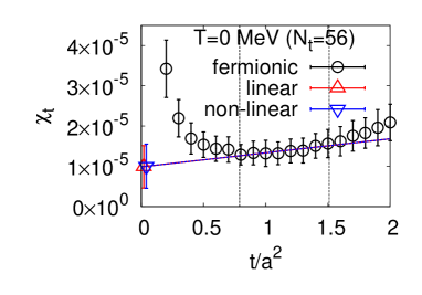
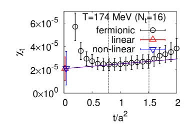
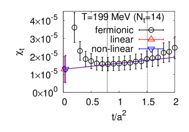
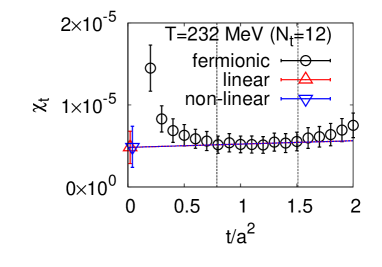
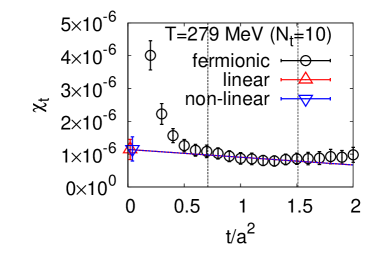
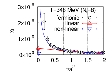
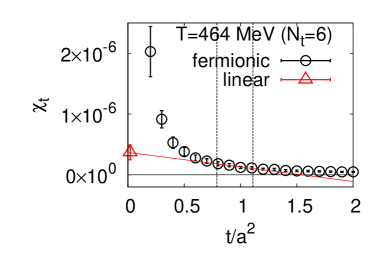
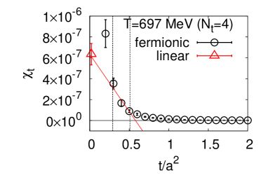
Figure 3: $\chi_{\mathrm{t}}(t,a)$ with the fermionic definition as a function of the flow time $t/a^{2}$. From the top left: $T\simeq 0$, $174$, $199$, $232$, $279$, $348$, $464$, and $697$ MeV, respectively. Vertical axis is in lattice unit. Pairs of vertical dotted lines indicate the window for the fit. The red solid lines with upward triangles are the results of the linear fit. The blue dotted lines with downward triangles are the results of the nonlinear fit discussed in the text.

In order to check the validity of the linear window and to estimate a systematic error due to the fit ansatz, we also try a nonlinear fit of the form

$$\chi_{\mathrm{t}}(t,a) = \chi_{\mathrm{t}}+A\frac{a^{2}}{t}+tB+Ct^{2}$$ (21)

adopting the same windows for the fit range. We restrict $A\geq 0$ and $C\geq 0$ to reproduce the increasing behavior of the data at small and large $t/a^{2}$ as seen in Fig. 3. The results of the nonlinear fit are shown by blue dotted lines with downward triangles in Fig. 3. We find that the coefficients $A$ and $C$ are very small and consistent with zero for $T\mathrel{\hbox to0.0pt{\raise 2.20013pt\hbox{$<$}\hss}{\lower 2.20013pt\hbox{$\sim$}}}279$ MeV, confirming the validity of the linear fit using the linear window. At $T\simeq 348$ MeV, on the other hand, we find a slight deviation from the linear fit, which we take as a systematic error in our final result. For $T\mathrel{\hbox to0.0pt{\raise 2.20013pt\hbox{$>$}\hss}{\lower 2.20013pt\hbox{$\sim$}}}464$, the nonlinear fit is not applicable because the number of data points within the window is not sufficient. Because the linear fits are also not reliable for these temperatures, we just disregard the results at $T\mathrel{\hbox to0.0pt{\raise 2.20013pt\hbox{$>$}\hss}{\lower 2.20013pt\hbox{$\sim$}}}464$.

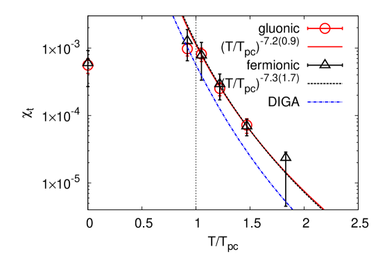
Figure 4: Topological susceptibility as a function of temperature. Vertical axis is in unit of $({\rm GeV})^{4}$.

Our results of $\chi_{\mathrm{t}}$ with the gluonic and fermionic definitions are summarized in Fig. 4 and Table 2. We find that the results from both definitions agree well with each other for $T\mathrel{\hbox to0.0pt{\raise 2.20013pt\hbox{$<$}\hss}{\lower 2.20013pt\hbox{$\sim$}}}279$ MeV ($T/T_{\mathrm{pc}}\mathrel{\hbox to0.0pt{\raise 2.20013pt\hbox{$<$}\hss}{\lower 2.20013pt\hbox{$\sim$}}}1.47$).

$T$ (MeV)	$T/T_{\mathrm{pc}}$	$\chi_{\mathrm{t}}^{\rm gluonic}$	$\chi_{\mathrm{t}}^{\rm fermionic}$
$0$	$0$	$0.00056(14)$	$0.00060(32)(^{+3}_{-4})(0)$
$174$	$0.92$	$0.00098(21)$	$0.00127(61)(^{+7}_{-14})(0)$
$199$	$1.05$	$0.00082(18)$	$0.00078(43)(^{+4}_{-9})(0)$
$232$	$1.22$	$0.000251(55)$	$0.00029(12)(^{+1}_{-2})(0)$
$279$	$1.47$	$0.000072(18)$	$0.000069(19)(^{+3}_{-4})(0)$
$348$	$1.83$	NA	$0.0000235(47)(21)(^{+0}_{-183})$
$464$	$2.44$	NA	NA
$697$	$3.67$	NA	NA

Table 2: The topological susceptibility $\chi_{\mathrm{t}}$ with the gluonic and fermionic definitions. The unit is $({\rm GeV})^{4}$. The number in the first parenthesis is the statistical error estimated by a jackknife method. For the fermionic definition, the second parenthesis is the systematic error due to the perturbative coefficients (18) and the running mass in (17), and the third parenthesis is the systematic error from the fit ansatz estimated by the difference between the linear and nonlinear fits.

Finally, we fit the data of $\chi_{\textrm{t}}$ at $T/T_{\mathrm{pc}}\simeq 1.05$–$1.47$ with a power low $(T/T_{\mathrm{pc}})^{-\gamma}$. The results are shown by red solid and black dashed curves for gluonic and fermionic definitions, respectively in Fig. 4. For the exponent, we find $\gamma=7.2(0.9)$ and $7.3(1.7)$ with the gluonic and fermionic definitions, respectively. These numbers are perfectly consistent with the one-loop DIGA prediction $\gamma\simeq 7.5$ at $T/T_{\mathrm{pc}}\simeq 1.5$. They agree even with the DIGA prediction $\gamma=8$ in the high temperature limit within statistical errors. On the other hand, the absolute value of $\chi_{\mathrm{t}}$ is slightly larger than a prediction of DIGA (the blue dot-dashed curve in Fig. 4). The DIGA prediction is given by an integration over the instanton size $\rho$

$$\chi_{\mathrm{t}}(T)=2\int_{0}^{\infty}\frac{d\rho}{\rho^{5}}\,n_{G}(\rho)\,n_{F}(m_{ud}\rho)\,n_{T}(\pi\rho T)$$ (22)

where $n_{G}$, $n_{F}$, and $n_{T}$ are the gauge, fermion, and finite temperature contributions, respectively, whose explicit forms are given by an instanton calculation tHooft:1976snw ; Gross:1980br and are summarized in Ref. frison . Inputs for the calculation are the pseudocritical temperature $T_{\mathrm{pc}}=190$ MeV, the QCD scale $\Lambda_{\textrm{QCD}}^{\overline{\rm MS}}=332(19)$ MeV Agashe:2014kda and the bare quark mass for which we adopted our PCAC mass of the up and down quarks. The $\overline{\rm MS}$ scheme is used with the renormalization scale which we set to $\mu=2\pi T$.

V Conclusion and discussion

We study temperature dependence of the topological susceptibility with the gradient flow method in (2+1)-flavor QCD with heavy $u$ and $d$ quarks, $m_{\pi}/m_{\rho}\simeq 0.63$, at a single but fine lattice spacing $a\simeq 0.07$ fm. We find that the results with the gluonic and fermionic definitions agree well with each other for $T\mathrel{\hbox to0.0pt{\raise 2.20013pt\hbox{$<$}\hss}{\lower 2.20013pt\hbox{$\sim$}}}279$ MeV even with the Wilson-type quarks whose numerical cost is much less than the Ginsparg-Wilson lattice quarks. Although the continuum extrapolation is not taken yet, the good agreement of different methods suggests that our lattices are already close to the continuum limit and the results are quantitatively reliable, in accordance with the observation of Ref. ourEOSpaper based on the results of the equation of state and the chiral condensate with gradient flow. At higher temperatures, we encountered several difficulties due to small $N_{t}$ and due to topological freezing. For the former, we need to decrease $a$. For the latter, a new idea such as the proposal of Ref. frison is needed.

Our topological susceptibility at $T/T_{\mathrm{pc}}\simeq 1.05$–$1.47$ show a power low behavior $\chi_{\mathrm{t}}\propto(T/T_{\mathrm{pc}})^{-\gamma}$ with exponent consistent with the prediction of the DIGA within statistical errors. Here, we note that there are discrepancies among our results and previous results, such as $\gamma=5.98(12)$ and $7.84(88)$ of Ref. Petreczky:2016vrs for the gluonic and fermionic definitions, respectively, in a similar temperature region, obtained with improved staggered quarks after taking a continuum extrapolation. To investigate a source of the discrepancy, we need to repeat the study at lighter quark mass and different lattice spacings. Studies are going on at a $m_{ud}$ close to the physical point and at different lattice spacings.

- (1) R. D. Peccei and H. R. Quinn, Phys. Rev. Lett. 38, 1440 (1977). doi:10.1103/PhysRevLett.38.1440
- (2) J. Preskill, M. B. Wise and F. Wilczek, Phys. Lett. B 120, 127 (1983)
- (3) L. F. Abbott and P. Sikivie, Phys. Lett. B 120, 133 (1983)
- (4) M. Dine and W. Fischler, Phys. Lett. B 120, 137 (1983)
- (5) G. ’t Hooft, Phys. Rev. D 14, 3432 (1976) Erratum: [Phys. Rev. D 18, 2199 (1978)]. doi:10.1103/PhysRevD.18.2199.3, 10.1103/PhysRevD.14.3432
- (6) D. J. Gross, R. D. Pisarski and L. G. Yaffe, Rev. Mod. Phys. 53, 43 (1981). doi:10.1103/RevModPhys.53.43
- (7) E. Berkowitz, M. I. Buchoff and E. Rinaldi, Phys. Rev. D 92, no. 3, 034507 (2015). doi:10.1103/PhysRevD.92.034507 [arXiv:1505.07455 [hep-ph]].
- (8) R. Kitano and N. Yamada, J. High Energy Phys. 1510, 136 (2015). doi:10.1007/JHEP10(2015)136 [arXiv:1506.00370 [hep-ph]].
- (9) S. Borsanyi, M. Dierigl, Z. Fodor, S.D. Katz, S.W. Mages, D. Nogradi, J. Redondo, A. Ringwald, and K.K. Szabo, Phys. Lett. B 752, 175 (2016). doi:10.1016/j.physletb.2015.11.020 [arXiv:1508.06917 [hep-lat]].
- (10) C. Bonati, M. D’Elia, M. Mariti, G. Martinelli, M. Mesiti, F. Negro, F. Sanfilippo and G. Villadoro, J. High Energy Phys. 1603, 155 (2016), doi:10.1007/JHEP03(2016)155 [arXiv:1512.06746 [hep-lat]].
- (11) P. Petreczky, H. P. Schadler and S. Sharma, Phys. Lett. B 762, 498 (2016). dx.doi.org/10.1016/j.physletb.2016.09.063 [arXiv:1606.03145 [hep-lat]].
- (12) S. Borsanyi et al., Nature 539, no. 7627, 69 (2016) doi:10.1038/nature20115 [arXiv:1606.07494 [hep-lat]].
- (13) R. Narayanan and H. Neuberger, J. High Energy Phys. 0603, 064 (2006), doi:10.1088/1126-6708/2006/03/064 [hep-th/0601210].
- (14) M. Lüscher, Commun. Math. Phys. 293, 899 (2010), doi:10.1007/s00220-009-0953-7 [arXiv:0907.5491 [hep-lat]].
- (15) M. Lüscher, J. High Energy Phys. 1008, 071 (2010); Erratum: [J. High Energy Phys. 1403, 092 (2014)], doi:10.1007/JHEP08(2010)071, 10.1007/JHEP03(2014)092 [arXiv:1006.4518 [hep-lat]].
- (16) M. Lüscher and P. Weisz, J. High Energy Phys. 1102, 051 (2011), doi:10.1007/JHEP02(2011)051 [arXiv:1101.0963 [hep-th]].
- (17) M. Lüscher, J. High Energy Phys. 1304, 123 (2013), doi:10.1007/JHEP04(2013)123 [arXiv:1302.5246 [hep-lat]].
- (18) M. Lüscher, Proc. Sci. LATTICE 2013, 016 (2014) [arXiv:1308.5598 [hep-lat]].
- (19) L. Giusti, G. C. Rossi and M. Testa, Phys. Lett. B 587, 157 (2004) doi:10.1016/j.physletb.2004.03.010 [hep-lat/0402027].
- (20) M. Lüscher, Phys. Lett. B 593, 296 (2004) doi:10.1016/j.physletb.2004.04.076 [hep-th/0404034].
- (21) L. Giusti and M. Lüscher, J. High Energy Phys. 0903, 013 (2009) doi:10.1088/1126-6708/2009/03/013 [arXiv:0812.3638 [hep-lat]].
- (22) M. Lüscher and F. Palombi, J. High Energy Phys. 1009, 110 (2010) doi:10.1007/JHEP09(2010)110 [arXiv:1008.0732 [hep-lat]].
- (23) Y. Taniguchi, S. Ejiri, R. Iwami, K. Kanaya, M. Kitazawa, H. Suzuki, T. Umeda, and N. Wakabayashi, arXiv:1609.01417 [hep-lat].
- (24) H. Suzuki, Progr. Theor. Exp. Phys. 2013, 083B03 (2013) Erratum: [Progr. Theor. Exp. Phys. 2015, 079201 (2015)] doi:10.1093/ptep/ptt059, 10.1093/ptep/ptv094 [arXiv:1304.0533 [hep-lat]].
- (25) H. Makino and H. Suzuki, Progr. Theor. Exp. Phys. 2014, 063B02 (2014) Erratum: [Progr. Theor. Exp. Phys. 2015, 079202 (2015)] doi:10.1093/ptep/ptu070, 10.1093/ptep/ptv095 [arXiv:1403.4772 [hep-lat]].
- (26) K. Hieda and H. Suzuki, Mod. Phys. Lett. A 31, no. 38, 1650214 (2016) doi:10.1142/S021773231650214X [arXiv:1606.04193 [hep-lat]].
- (27) T. Ishikawa, S. Aoki, M. Fukugita, S. Hashimoto, K.-I. Ishikawa, N. Ishizuka, Y. Iwasaki, K. Kanaya, T. Kaneko, Y. Kuramashi, M. Okawa, Y. Taniguchi, N. Tsutsui, A. Ukawa, N. Yamada, and T. Yoshiè [CP-PACS and JLQCD Collaborations], Phys. Rev. D 78, 011502(R) (2008), doi:10.1103/PhysRevD.78.011502 [arXiv:0704.1937 [hep-lat]].
- (28) T. Umeda, S. Aoki, S. Ejiri, T. Hatsuda, K. Kanaya, H. Ohno, and Y. Maezawa [WHOT-QCD Collaboration], Phys. Rev. D 85, 094508 (2012), doi:10.1103/PhysRevD.85.094508 [arXiv:1202.4719 [hep-lat]].
- (29) Y. Iwasaki, arXiv:1111.7054 [hep-lat].
- (30) L. Levkova, T. Manke, and R. Mawhinney, Phys. Rev. D 73, 074504 (2006), doi:10.1103/PhysRevD.73.074504 [hep-lat/0603031].
- (31) T. Umeda, S. Ejiri, S. Aoki, T. Hatsuda, K. Kanaya, Y. Maezawa and H. Ohno, Phys. Rev. D 79, 051501 (2009), doi:10.1103/PhysRevD.79.051501 [arXiv:0809.2842 [hep-lat]].
- (32) M. Garcia Perez, O. Philipsen and I. O. Stamatescu, Nucl. Phys. B 551, 293 (1999) doi:10.1016/S0550-3213(99)00211-4 [hep-lat/9812006].
- (33) C. Bonati and M. D’Elia, Phys. Rev. D 89, no. 10, 105005 (2014) doi:10.1103/PhysRevD.89.105005 [arXiv:1401.2441 [hep-lat]].
- (34) Y. Namekawa, Proc. Sci. LATTICE 2014, 344 (2015) [arXiv:1501.06295 [hep-lat]].
- (35) C. Alexandrou, A. Athenodorou and K. Jansen, Phys. Rev. D 92, no. 12, 125014 (2015) doi:10.1103/PhysRevD.92.125014 [arXiv:1509.04259 [hep-lat]].
- (36) A. Ali Khan et al. [CP-PACS Collaboration], Phys. Rev. D 64, 114501 (2001) doi:10.1103/PhysRevD.64.114501 [hep-lat/0106010].
- (37) M. Cé, C. Consonni, G. P. Engel and L. Giusti, Phys. Rev. D 92, 074502 (2015), doi:10.1103/PhysRevD.92.074502 [arXiv:1506.06052 [hep-lat]].
- (38) M. Lüscher, talk given at “Workshop on Chiral Dynamics with Wilson Fermions”, Trento, 24-28 October 2011.
- (39) M. Bochicchio, G. C. Rossi, M. Testa and K. Yoshida, Phys. Lett. B 149, 487 (1984). doi:10.1016/0370-2693(84)90372-1
- (40) J. Frison, R. Kitano, H. Matsufuru, S. Mori, and N. Yamada, arXiv:1606.07175 [hep-lat].
- (41) S. Bethke, G. Dissertori and G.P. Salam (Particle Data Group), 2015, Chapt. 9, Quantum Chromodynamics, http://pdg.lbl.gov/2015/reviews/rpp2015-rev-qcd.pdf
- (42) http://bridge.kek.jp/Lattice-code/index_e.html