Fe K and ejecta emission in SNR G15.9+0.2 with XMM-Newton

Abstract

Aims. We present a study of the Galactic supernova remnant SNR G15.9+0.2 with archival XMM-Newton observations.

Methods. EPIC data are used to investigate the morphological and spectral properties of the remnant, searching in particular for supernova ejecta and Fe K line emission. By comparing the SNR’s X-ray absorption column density with the atomic and molecular gas distribution along the line of sight, we attempt to constrain the distance to the SNR.

Results. Prominent line features reveal the presence of ejecta. Abundance ratios of Mg, Si, S, Ar, and Ca strongly suggest that the progenitor of SNR G15.9+0.2 was a massive star with a main sequence mass likely in the range 20–25 $M_{\sun}$, strengthening the physical association with a candidate central compact object detected with Chandra. Using EPIC’s collective power, Fe K line emission from SNR G15.9+0.2 is detected for the first time. We measure the line properties and find evidence for spatial variations. We discuss how the source fits within the sample of SNRs with detected Fe K emission and find that it is the core-collapse SNR with the lowest Fe K centroid energy. We also present some caveats regarding the use of Fe K line centroid energy as a typing tool for SNRs. Only a lower limit of 5 kpc is placed on the distance to SNR G15.9+0.2, constraining its age to $t_{SNR}\gtrsim 2$ kyr.

1 Introduction

SNR G15.9+0.2 was discovered as a supernova remnant (SNR) at radio wavelengths in Molonglo-Parkes observations by Clark et al. (1973, 1975). Higher spatial resolution radio observations with VLA revealed the elongated shell-like structure of the SNR with a bright enhancement on the eastern border (Dubner et al. 1996). The source is relatively bright in X-rays, as found in Chandra data by Reynolds et al. (2006b, hereafter R06). Its X-ray morphology favours a core-collapse (CC) origin according to Lopez et al. (2009, 2011). The SNR was detected in infrared with Spitzer/MIPS by Pinheiro Gonçalves et al. (2011), who measured a dust temperature and mass of 60 K and $8.1\times 10^{-2}$ $M_{\sun}$, respectively.

Although 300 SNRs are now known in the Milky Way, SNR G15.9+0.2 is an interesting target for an in-depth analysis for several reasons. First, it is likely young, $\sim 10^{3}$ yr according to R06, as suggested by its small angular diameter and Chandra X-ray analysis. This could add SNR G15.9+0.2 to the small sample (about 15) of SNRs confirmed to be $\lesssim 2000$ yr old (using the compilation  of Ferrand & Safi-Harb 2012) and thus reduces the discrepancy between the observed and expected numbers of young SNRs. Second, a compact source, identified as CXOU~J181852.0$-$150213, was discovered in the central region of the SNR (R06) with X-ray properties typical of central compact objects (CCOs, e.g. Pavlov et al. 2004). Recently, deeper Chandra observations allowed Klochkov et al. (2016) to confirm that the central object is indeed a young cooling low-magnetized neutron star. This adds SNR G15.9+0.2 to the short list of seven SNRs hosting a confirmed CCO and as many hosting bona fide candidates (Lazendic et al. 2005; De Luca et al. 2006; de Luca 2008; Halpern & Gotthelf 2010; Combi et al. 2010; Sánchez-Ayaso et al. 2012). Third, its young age and plasma conditions should produce detectable Fe K emission. This feature is a blend of lines from various Fe ions, with a centroid energy at $\sim 6.4$ keV for ionisation states lower than Fe¹⁷⁺, and then progressing to $\sim 6.7$ keV for ion charges up to 24. The ionic fraction of iron, and thus the centroid energy of the Fe K line, is chiefly governed by the ionisation timescale $n_{e}t$, where $n_{e}$ is the electron density and $t$ the time since the plasma was shocked. After analysing all SNRs observed with Suzaku, Yamaguchi et al. (2014, hereafter Y14) detected Fe K emission from 16 Galactic and seven LMC SNRs. They showed that the Fe K centroid energy discriminates type Ia and CC SNRs, with the former consistently in the lower end ($\sim 6.4$ keV) of the ionisation range, and CC SNRs closer to 6.7 keV. They attributed this to CC SNRs expanding into higher density environments produced by the massive star prior to the explosion, while the ambient medium around type Ia SNRs is hardly modified by the SN progenitors. If Fe K emission from SNR G15.9+0.2  were detected, we could obtain independent clues to the origin of the remnant.

SNR G15.9+0.2 was serendipitously observed in XMM-Newton pointings of a neighbouring target. Thanks to its superior collective power, there are several points where results from R06 can be elaborated upon and improved. In particular, the effective area of EPIC-pn is five times higher than Chandra’s ACIS at 6.4 keV, making it a prime instrument to search for faint Fe K emission yet undetected. The Chandra image revealed an incomplete shell in X-rays, broken in the north-west quadrant, while radio emission is still found there. With XMM-Newton we can look for and characterise X-ray emission to much fainter limits. Furthermore, the SNR is bright and extended enough ($\sim 5.5$′ across) so that even with the modest angular resolution offered by XMM-Newton, we can measure abundances and plasma conditions in various regions around the remnant. The derived abundance ratios can constrain the type of progenitor and provide additional hints to the origin of the SNR. Finally, using X-ray spectral analysis and other tracers (namely atomic and molecular gas), we can reassess the age of the SNR and the measurements of its distance.

This work is organised as follows: We first present the observations and data reduction in Sect. 2. Next, we describe in Sect. 3 the results of the morphological and spectral analyses. In Sect. 4, we discuss the type of progenitor, age, and distance to SNR G15.9+0.2, as well as the evolution of Fe K lines in SNRs in general. We summarise our findings in Sect. 5.

Table 1: Details of the X-ray observations

ObsID	Date	Total / filtered $t_{\mathrm{exp}}$	Mode
0406450201	2006 Apr 6	43 / 33	SW
0505240101	2008 Mar 31	93 / 47	FF

2 X-ray observations and data reduction

SNR G15.9+0.2 was in the field of view (FoV) of two XMM-Newton observations targeting PSR J1819$-$1458, the first X-ray counterpart to a Rotating RAdio Transients (RRATs, Reynolds et al. 2006a; McLaughlin et al. 2007; Miller et al. 2013). The SNR is located at off-axis angles ranging from 8′ to 12′. Only MOS data are available for the first observation, which was performed with EPIC in small window (SW) mode (the outer MOS CCDs are active even in SW mode). We discarded two additional observations that were very short ($\lesssim 5$ ks). Details of the observations used in this paper are listed in Table 1.

We used the XMM SAS  version 14.0.0 for the data reduction. We applied a threshold of 8 and 2.5 cts ks^-1 arcmin^-2 on pn and MOS light curves in the 7–15 keV energy band to screen out periods of high background activity. This resulted in useful exposure times of 47 ks and 33 ks.

We created two sets of images and exposure maps in various energy bands from the filtered event lists: A “broad band” set covering 0.2 keV to 12 keV in five bands as given in Watson et al. (2009, their Table 3), and an “SNR” set described in Sect. 3.1. Single and double-pixel events ($0\leq$ PATTERN $\leq 4$) were extracted from the pn detector, while all valid events from the MOS detectors were selected ($0\leq$ PATTERN $\leq 12$). Masks were applied to filter out bad pixels and columns. The SAS task edetectchain is applied simultaneously to the five images of the broad band set to identify X-ray (point) sources in each observations. The detection lists were primarily used to exclude unrelated point sources from the spectrum extraction regions.

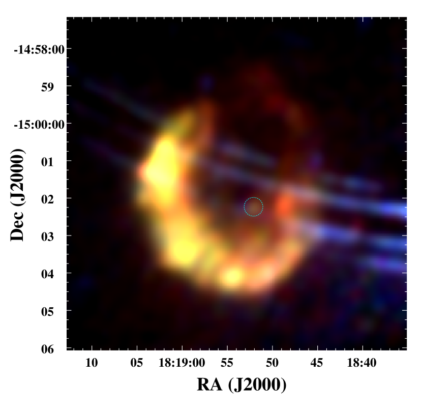
Figure 1: X-ray colour image of SNR G15.9+0.2, combining pn and MOS data. The red, green, and blue components are soft, medium, and hard X-rays, as defined in Sect. 3.1. The position of the CCO is circled in cyan. The blue arcs are straylight contamination (see Sect. 3.2).

3 Results

3.1 Morphology

To study the morphology of SNR G15.9+0.2, we used three energy bands tailored to its spectrum (R06). A soft band from 0.9 to 2.1 keV which includes strong lines from magnesium and silicon; a medium band from 2.1 to 3.25 keV which comprises sulphur and argon lines; and a hard band (3.25–7.2 keV) which includes the high-energy part of the continuum and possibly emission from calcium and Fe K lines. Owing to high absorption, there is little emission below 0.8 keV, while the instrumental background dominates above 7.2 keV.

We used filter wheel closed (FWC) data , obtained with the detector shielded from astrophysical background, to subtract the detector background. The contribution of detector background in each observation was estimated from the count rate in the corners of the images, since they are not exposed to the sky. We then subtracted appropriately scaled FWC data from the raw images. The detector background-subtracted images from the two observations were merged together. They were then adaptively smoothed: the sizes of Gaussian kernels were chosen at each position to reach a signal-to-noise ratio of five, with a minimum full width at half maximum (FWHM) of 20″. In each band, we co-added the smoothed images from pn and MOS, and divided the resulting image by the corresponding vignetted exposure map .

The composite X-ray image of SNR G15.9+0.2 is shown in Fig. 1. The annular stripes at high energy (in blue) are straylight emission (see Sect. 3.2) unrelated to the SNR. The position of the CCO is marked. A faint point source is detected 2″ from CXOU J181852.0$-$150213, i.e. well within the typical XMM-Newton statistical and systematical position uncertainties. The flux and hardness ratios are consistent with those measured with Chandra (R06) so we are confident that we are indeed detecting the CCO. However, there are not enough counts ($\lesssim 200$) to improve on results from R06 or Klochkov et al. (2016), especially with the lower angular resolution of XMM-Newton.

SNR G15.9+0.2 exhibits a well-defined shell morphology. The eastern and south-western edges are particularly bright, and all the SNR emission above $\sim 3.5$ keV is concentrated in these regions. In contrast, the north-western quadrant of the shell is much fainter than the rest of the SNR, and only X-rays below 3 keV are detected in this region. The shell’s morphology is a slightly elongated ellipse, with major and minor axes of 6.2′ and 5.2′, respectively. That translates into a linear size of (9.0 pc $\times$ 7.6 pc) ($D$ / 5 kpc). The major axis has a position angle 150° eastwards of north. The centre of the ellipse is at RA (J2000) = 18^h 18^m 53.8^s, DEC = $-$15° 01^m 38^s. The CCO is thus offset 44″ from the visual centre.

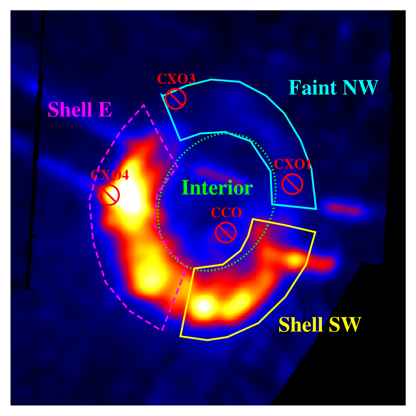
Figure 2: Regions used in the spectral analysis defined on a 0.9-7.2 keV band image of SNR G15.9+0.2. Point sources in red were excluded. We note the changing straylight contamination in different regions.

3.2 Spectral analysis

The definition of extraction regions for spectral analysis was driven by the observed morphology. A spatially integrated spectra was extracted from the ellipse described previously. To look for spectral variations, we separated the bright regions of the shell in two subregions, “Shell E” and “Shell SW” (for east and south-west, respectively). These are shown over an X-ray image in Fig. 2. A third region covers the fainter north-western part of the shell (“faint NW”). We also extracted a spectrum from the interior of the SNR.

Point sources detected with Chandra , including the CCO, were excised from our XMM-Newton spectral extraction regions. Most of the sources detected with XMM-Newton in the shell region (by edetectchain) are emission knots, therefore truly originating from the SNR and were kept in the analysis. Background spectra were taken from a large region surrounding the SNR (not shown in Fig. 2). We excluded straylight stripes and point sources detected with XMM-Newton from the background regions.

Owing to the telescope vignetting and off-axis position of the SNR, the effective area changes across the extent of the SNR; it decreases with larger off-axis angles, and more so at higher energies. Before extracting spectra, we corrected the filtered event lists for vignetting with the SAS task evigweight. As for the images, single and double-pixel events were included in pn spectra, and events with PATTERN = 0 to 12 were selected in MOS spectra. With the FTOOLS task grppha, we rebinned all spectra to have a minimum of 25 counts per bin in order to allow the use of the $\chi^{2}$-statistic. Non-rebinned spectra were used with the C-statistic (Cash 1979) for the study of Fe K lines (Sect. 3.2.2) because of the limited photon statistics above 6 keV. These spectra were extracted from non-vignetting-weighted event lists to retain the Poissonian nature of the errors. XSPEC (Arnaud 1996) version 12.9.0e was used for the spectral analysis. All uncertainties listed in this paper are given at the 90% confidence level, unless otherwise stated.

For spectral analysis, we employed the method described in Maggi et al. (2016): We simultaneously fit the source and background spectra with the instrumental and astrophysical contributions to the background explicitly modelled. This is preferable to simply subtracting a background spectrum taken from a nearby region because of the different instrumental responses and background contributions from different regions and because of the resulting loss in the statistical quality of the source spectrum.

Spectra were extracted from FWC data at the same detector positions as the source and background regions, in order to capture the spatial variations of the instrumental background. Our model for the instrumental background takes into account electronic noise and particle-induced background, as described in Sturm (2012) and Maggi et al. (2016). We first fit this model to FWC data from all extraction regions. The best-fit models are used in subsequent fits (including astrophysical signal), allowing only a constant renormalisation factor. This avoids overloading the number of free parameters. Another non-X-ray background component is the soft proton contamination (SPC), which we modelled following the prescription of Kuntz & Snowden (2008). The SPC parameters were different for each instrument and observation (the soft proton flux is highly time-variable). Indeed, we found a higher SPC in the 2006 observation.

Next, we defined a model for the astrophysical X-ray background (AXB). Initially, we used a single unabsorbed thermal plasma (apec in XSPEC) for local contributions (local hot bubble and/or solar wind charge-exchange emission) and an absorbed two-temperature plasma (apec + apec) for the remote (Galactic) component. The cosmic X-ray background is added, with additional absorption, to the remote component as a power law with a photon index $\Gamma$ fixed to 1.41 (De Luca & Molendi 2004). Initial trial fits to the background spectra showed that a second remote Galactic component was not needed. This usually accounts for the very hot ($kT>5$ keV) plasma from the Galactic ridge X-ray emission (GRXE), which is not detected in our data. In particular, we do not see the strong Fe K line at 6.7 keV associated with the GRXE (Koyama et al. 1986). We place a $3\sigma$ upper limit of $2.8\times 10^{-8}$ ph cm^-2 s^-1 arcmin^-2 on a Galactic ridge Fe K line. Below 1 keV, the initial model had strong residuals. A much better fit was achieved with the inclusion of a second thermal component. The final model for the AXB is

$$S_{\mathrm{AXB}}=S^{1}_{\mathrm{apec}}+S^{2}_{\mathrm{apec}}+\mathrm{\texttt{phabs}}(N_{H}^{1})\left(S^{3}_{\mathrm{apec}}+\mathrm{\texttt{phabs}}(N_{H}^{2})N_{\mathrm{CXB}}E^{-\Gamma}\right)$$ (1)

where $S^{i}_{\mathrm{apec}}$ is the emission from an apec model at temperature $kT^{i}$ with normalisation $Norm^{i}$. The latter is defined as $(10^{-14}/4\pi D^{2})\int n_{e}n_{H}dV$, with $D$ the distance to the source and $n_{e}$ and $n_{H}$ the density of electrons and protons, all in the cgs system of units. phabs is the photoelectric absorption model we used in XSPEC, with cross-sections from Balucinska-Church & McCammon (1992). Abundances were set to those of Wilms et al. (2000).

The model of Eq. 1 reproduces fairly well the background spectrum (see Fig. 3). The best-fit parameters are listed in Table 2. Our CXB surface brightness is an order of magnitude higher than derived at high Galactic latitudes from various instruments (Kushino et al. 2002; Lumb et al. 2002; De Luca & Molendi 2004; Revnivtsev et al. 2005). This can be attributed partly to cosmic variance, and partly to contribution by unresolved hard X-ray sources in the Galaxy which are by design not in the aforementioned CXB studies. We note that Katsuda et al. (2015) fit the CXB on a background spectrum around RX J1713.7-3946, located symmetrically from SNR G15.9+0.2 with respect to the Galactic Centre. Their value of $(1.0-3.2)\times 10^{-5}$ ph keV^-1 cm^-2 s^-1 arcmin^-2 at 1 keV is fully consistent with ours ($1.6\times 10^{-5}$).

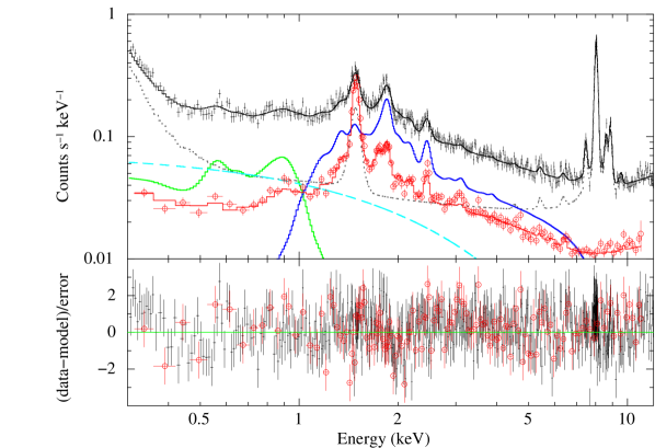
Figure 3: Background spectrum of SNR G15.9+0.2. For the sake of clarity, only pn and MOS2 data from the 2008 observation are shown (black and red points, respectively). Data have been rebinned for display purposes. The various components are instrumental background (dotted grey), local background (solid green), remote background and CXB (solid blue) and SPC (dashed cyan). Fit residuals are displayed in the bottom panel.

Another potentially problematic source of background is straylight. Photons from bright sources outside the FoV can be singly reflected by the hyperboloid mirrors and reach the camera. Sources 0.3° to 1.4° off-axis produce ring-like structures in EPIC images , such as seen in our images. Following the direction to the foci of the straylight rings from the aimpoint of the observations, we can firmly identify the contaminating source as GX 17+2, located 1.26° off-axis. GX 17+2 is a low-mass X-ray binary accreting at Eddington luminosity (e.g. Lin et al. 2012, and references therein). Excising straylight rings from the background extraction regions is straightforward. However, some single-reflection arcs also intersect (bright) regions of the SNR. We therefore chose to include another component to model the straylight emission possibly included in the spectra from the SNR regions. To analyse the straylight spectrum, we extracted counts from the ring-like structures in all the FoV, except over SNR G15.9+0.2. The spectrum of GX 17+2 can be represented as a combination of black body, multicolour disk, and power-law emission, with variable relative contributions (Cackett et al. 2010; Lin et al. 2012) depending on the state of GX 17+2, although a single component model is sufficient given the limited count statistics of the single reflections. We note in particular that we do not see Fe K emission from GX 17+2 (Cackett et al. 2012) in the straylight spectrum, which has almost no signal above 6 keV. We used an absorbed black body with $N_{H}=3.1\times 10^{22}$ cm^-2 and $kT=0.99$ keV. The normalisation is free for all exposures, as it depends on both the intrinsic variability of the source and on its exact location relative to the mirrors. Overall, the flux collected in all the arcs is $10^{-4}-10^{-3}$ times the flux of GX 17+2, consistent with the straylight collecting area (<0.2 % of the on-axis effective area). We included this component in the background model of spectra in the source regions. The spectral parameters were fixed. A constant factor was the only free parameter allowed to vary between 0 (no contribution) and $f_{\mathrm{stray}}$, where $f_{\mathrm{stray}}$ is a geometrical factor, the fraction of the straylight arc overlapping the SNR region.

Table 2: Best-fit parameters for the AXB model of Eq. 1.

Parameter	Value
$\chi^{2}$ / d.o.f ($\chi^{2}_{r}$) $=3089.8/2712\ (1.14)$
Local background
$kT^{1}$ (keV)	$0.19\pm 0.02$
$Norm^{1}$ (cm-5)	$(1.95\pm 0.22)\times 10^{-5}$
SB1 (erg cm-2 s-1 arcmin-2)	$1.8\times 10^{-15}$
$kT^{2}$ (keV)	$0.84\pm 0.04$
$Norm^{2}$ (cm-5)	$(1.95\pm 0.22)\times 10^{-5}$
SB2 (erg cm-2 s-1 arcmin-2)	$2.3\times 10^{-15}$
Remote background
$N_{H}^{1}$ ($10^{22}$ cm-2)	$3.14\pm 0.10$
$kT^{3}$ (keV)	$0.72\pm 0.03$
$Norm^{3}$ (cm-5)	$(5.05_{-0.56}^{+0.44})\times 10^{-3}$
SB3 (erg cm-2 s-1 arcmin-2)	$2.4\times 10^{-14}$
Cosmic X-ray background
$N_{H}^{2}$ ($10^{22}$ cm-2)	$1.25_{-0.73}^{+0.93}$
$\Gamma$	1.41 (fixed)
$N_{\mathrm{CXB}}$ (ph keV-1 cm-2 s-1 at 1 keV )	$(2.84\pm 0.13)\times 10^{-4}$
SBCXB (erg cm-2 s-1 arcmin-2)	$6.5\times 10^{-14}$

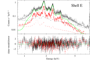
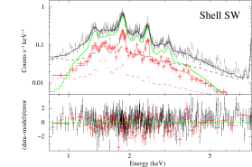
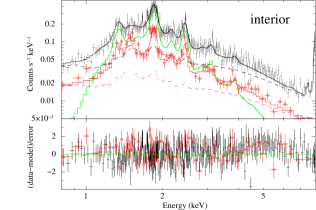
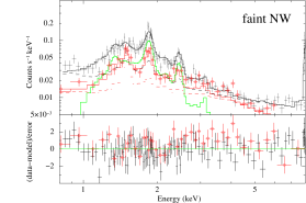
Figure 4: X-ray spectra from various regions of SNR G15.9+0.2, with pn and MOS2 data from the 2008 observation in black and red, respectively. All background components are included in the dashed lines (model from Fig. 3, plus straylight contamination, see Sect. 3.2). The best-fit fiducial model for the SNR emission is in green, with corresponding residuals in the bottom panels. We note the changing vertical scale between rows.

3.2.1 Spectral fits and spatial variations

In a first attempt, we fit single-temperature models to the spectra from each region, combining the background model and one or more components for the SNR emission. All background parameters are fixed to their best-fit values, except for normalisation factors for the AXB and the straylight models. We assumed non-equilibrium ionisation (NEI) for the SNR emission, using a plane-parallel shock model (vpshock in XSPEC, Borkowski et al. 2001), which features a linear distribution of ionisation ages ($\tau=\int_{0}^{t}n_{e}dt$). AtomDB 3.0  is used to calculate the spectrum.

We started with the “Shell E” spectrum from the brightest region. Initial fits with vpshock and solar abundances clearly failed, leaving strong residuals at line energies of main elements, in particular Si and S. With free Mg, Si, and S abundances, the fit improved by $\Delta\chi^{2}=-797$. Some residuals remained at $E\sim 3.2$ keV and 3.9 keV, where Ar and Ca emission is expected. With their abundances freed, the fit improved further by $\Delta\chi^{2}=-95$ for a final $\chi^{2}$ / d.o.f $=2191.2/1967$. The enhanced abundances are a tell-tale sign of the shock-heated ejecta origin of the emission. In all these fits there are line-like residuals at 6.4 keV – 6.7 keV, which betrays unaccounted for Fe K emission. It cannot be improved by enhanced Fe abundance, because the plasma temperature, constrained by the bulk of the emission, is too low to produce appreciable Fe K emission. Adding a Gaussian improved the fits; we analyse the Fe K emission in detail in Sect. 3.2.2.

Because the 6.4 keV feature is very minor, we restrict in a first time the analysis to the vpshock model with free Mg, Si, S, Ar, and Ca abundances as it gives a good fit to the the global emission that can be applied in all regions of the SNR. We refer to this model as the fiducial model. The best-fit parameters in each region are listed in Table 3.

Table 3: Best-fit parameters for the fiducial model.

Region	$N_{H}$	$kT$	$\tau$	Norm	$\chi^{2}$ / d.o.f.
	($10^{22}$ cm-2)	(keV)	($10^{10}$ s cm-3)	(cm-5)
Shell E	5.03${}_{-0.25}^{+0.21}$	1.32${}_{-0.09}^{+0.08}$	8.54${}_{-0.81}^{+0.99}$	$(1.32_{-0.14}^{+0.20})\times 10^{-2}$	2191.2/1967 (1.11)
Shell SW	4.30${}_{-0.27}^{+0.17}$	1.53${}_{-0.09}^{+0.28}$	7.69${}_{-1.25}^{+1.18}$	$(5.18_{-1.17}^{+0.58})\times 10^{-3}$	1980.2/1726 (1.15)
Interior	4.10${}_{-0.26}^{+0.12}$	1.46${}_{-0.21}^{+0.28}$	6.69${}_{-1.39}^{+1.56}$	$(3.15_{-0.74}^{+0.83})\times 10^{-3}$	1678.3/1632 (1.03)
Faint NW	3.77${}_{-0.35}^{+0.44}$	0.67$\pm 0.20$	96.8 $(>34.7)$	$(2.59_{-1.05}^{+3.13})\times 10^{-3}$	959.4/896 (1.07)
Integrated	4.58$\pm 0.11$	1.44${}_{-0.06}^{+0.08}$	7.85${}_{-0.60}^{+0.79}$	$(2.34_{-0.19}^{+0.16})\times 10^{-2}$	3860.4/3418 (1.13)
	Mg	Si	S	Ar	Ca
Shell E	1.79${}_{-0.25}^{+0.32}$	2.57 $(\pm 0.18)$	2.69 $(\pm 0.17)$	3.44${}_{-0.45}^{+0.51}$	2.53${}_{-1.02}^{+1.22}$
Shell SW	1.79${}_{-0.30}^{+0.40}$	2.06${}_{-0.17}^{+0.30}$	2.11${}_{-0.20}^{+0.29}$	2.73${}_{-1.24}^{+0.80}$	1.24 $(<3.05)$
Interior	1.83${}_{-0.33}^{+0.44}$	2.06${}_{-0.24}^{+0.32}$	2.03${}_{-0.27}^{+0.33}$	2.99${}_{-1.10}^{+1.27}$	6.68${}_{-3.62}^{+4.39}$
Faint NW	1.33${}_{-0.44}^{+0.60}$	1.66 $(\pm 0.40)$	2.04${}_{-0.57}^{+1.08}$	4.26${}_{-2.62}^{+6.71}$	3.49 $(<20.2)$
Integrated	1.74${}_{-0.18}^{+0.20}$	2.20${}_{-0.10}^{+0.13}$	2.29${}_{-0.11}^{+0.14}$	3.15${}_{-0.37}^{+0.42}$	2.49${}_{-0.91}^{+0.98}$

The temperature and ionisation age in the “Shell E” spectrum are 1.32 keV and $8.5\times 10^{10}$ cm s^-3. The spectrum in the “Shell SW” region is similar to its eastern counterpart, with a higher temperature (1.53 keV) but the same ionisation age within the uncertainties. The interior spectrum is virtually the same as that in the “Shell SW”, albeit fainter, indicating that we are seeing (in projection) similar shock conditions as in the south-west. The spectrum in the “faint NW” region is the most different; the temperature is significantly lower ($kT\approx 0.7$ keV) and the ionisation age is higher ($\tau\sim 8\times 10^{11}$ cm s^-3), although poorly constrained. The eastern emission is the most absorbed with a column density $N_{H}=5\times 10^{22}$ cm^-2, while $N_{H}$ is lower in the interior and south-west. The $N_{H}$ in the interior ($4.10^{+0.12}_{-0.26}\times 10^{22}$ cm^-2) is consistent with the value fit by Klochkov et al. (2016) for the CCO using a carbon atmosphere model, the only one that yields a reasonable distance ($10^{+9}_{-5}$ kpc). The X-ray emission from the north-west appears the least absorbed ($N_{H}\lesssim 4\times 10^{22}$ cm^-2). These absorption features are discussed in relation with atomic and molecular gas in Sect. 4.3.

The abundances are highly elevated (in excess of 1.5–2 times solar) in every region except the “faint NW”, where some abundances are consistent with solar when taking into account the large uncertainties. We do not find a solar value for Si, as did R06 in Chandra data fit with the same model. The abundances of Ar and Ca are, however, poorly constrained in spectra with lower statistics, in particular in the interior and north-western regions. Within the uncertainties, there are no clear spatial variations of the abundance ratios of Mg or S relative to Si. We also applied the fiducial model to the integrated spectrum of SNR G15.9+0.2. The resulting best-fit parameters are listed in Table 3. They are consistent with flux-averaging of the parameters obtained in the four regions.

It appears from the fiducial model that a significant fraction, or the majority, of the emission originates from shock-heated ejecta. Therefore, we attempted a multicomponent model approach (similar e.g. to that in Kosenko et al. 2010): A single $kT$ NEI component (vpshock) is used for each element or group of elements. This examines whether various elements are found at different temperatures or ionisation ages. To model emission from pure ejecta, we set the abundance of the corresponding element(s) to $10^{9}$ and all the others to 0. The model thus comprises i) a component for Mg; ii) a component for Si, S, Ar, and Ca. They are grouped together as they are expected to be roughly co-spatial in the ejecta of a (core-collapse) supernova. The abundances of S, Ar, and Ca are free relative to Si; iii) a component for iron, the innermost ejecta, which we detected through Fe K emission; and iv) an additional component with solar abundance to account for the emission from shocked ambient medium (hereafter solar component). All components share a common $N_{H}$.

This model was applied to the bright eastern and south-western spectra. Taking into account the seven additional free parameters, the fits with the multicomponent model are equally as good or slightly better than those with the fiducial model. Again, the $N_{H}$ is higher in the eastern region, confirming that this spatial variation is not strongly model dependent. The solar-abundances component dominates the continuum. It is therefore unsurprising that a pure-ejecta model (without the solar-abundances component) fails to describe the data satisfactorily. The temperature of the solar-abundances component is (1.3 – 1.5) keV without spatial variation in $\tau$, as with the fiducial model. The Si-group component has a lower temperature (0.9 – 1 keV) and higher $\tau$ ($2\times 10^{11}$ cm s^-3) than the solar and Mg components. Without the help of the absorbed iron L-shell lines below 1.2 keV, we cannot constrain well the $kT-\tau$ combination for Fe, an issue further complicated by the complex nature of the Fe K emission, as described in the next section.

3.2.2 Fe K emission

Here we present a separate treatment of the Fe K emission at 6.4 keV – 6.7 keV for comparison with the results of Y14. The same background model as previously described is included. Data between 0.6 keV and 4 keV are excluded, thus avoiding the prominent line emission from elements other than Fe. The low-energy part (from 0.3 to 0.6 keV) is used to fix the normalisation of the background model. The continuum emission is modelled by an absorbed Bremsstrahlung ($N_{H}$ fixed to $5\times 10^{22}$ cm^-2), and the Fe K emission by a Gaussian. There is only a significant detection of the line in the “Shell E” and “Shell SW” regions, and particularly in pn data. There is no clear signature in the MOS spectra owing to their lower effective area. Still, we present the results of the joint pn/MOS analysis since it helps in constraining the continuum. No differences were found in the line properties when using only pn data.

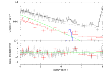
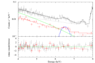
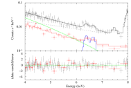
Figure 5: Spectrum of SNR G15.9+0.2 around 6.4 keV. The bremsstrahlung continuum is shown in green, Fe K emission in blue. Black points and line are the pn data and best-fit model, respectively. All other background contributions are shown by the dashed black line. As in Fig. 3, we only show one example for MOS (red). Residuals are displayed in the bottom panels. Models used for the iron emission (from left to right): Gaussian with width fixed to zero, Gaussian with free width, two Gaussians with width fixed to zero. See best-fit parameters in Table 4.

We start the analysis with the “Shell E” spectrum, which has the best signal. With a width fixed to zero , the best-fit Gaussian has a centroid energy of 6405${}_{-49}^{+52}$ eV (Table 4). However, this model leaves residuals around the centroid energy, as shown in Fig. 5 (left). When the width ($\sigma$) of the line is freed, the fit improves significantly ($\Delta$C$=-12$) for $\sigma=191_{-\ 72}^{+131}$ eV, with a centroid energy shifted to 6519${}_{-79}^{+81}$ eV (Fig. 5, middle). The data can be fit equally well or slightly better ($\Delta$C$=-5.3$) by using two zero-width Gaussians. In that case, one is at low energy ($\sim 6.4$ keV) and the second is close to 6.7 keV (Fig. 5, right). In the south-west region, only a narrow high-energy component is detected; there is no improvement when thawing the line width (Table 4). We note that in the population study of Y14, the Gaussian width was left free in all the fits (Hiroya Yamaguchi, personal communication).

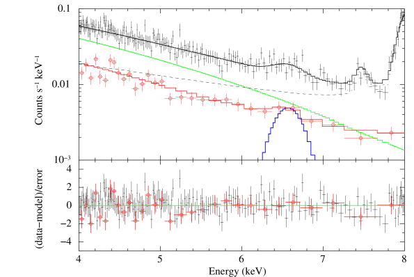
Figure 6: Same as Fig. 5 for the “Bright” region. The model used for the iron emission is a Gaussian with free width.

We also extracted a spectrum covering both the east and south-west regions (“Bright” region in Table 4), to measure the integrated properties of the Fe K emission without adding too much background from the interior and “faint NW” regions where the line is not detected. We found a best-fit centroid at 6577${}_{-70}^{+73}$ eV and width of 155${}_{-\ 57}^{+103}$ eV (Fig. 6). In this region, a good fit is also obtained with the two-Gaussian model, for centroids of 6411 $\pm 46$ eV and 6670${}_{-41}^{+34}$ eV and about the same flux for both components. The total flux in the line is $(6.1_{-1.9}^{+1.8})\times 10^{-6}$ photon cm^-2 s^-1, less than 8 % of which could be attributed to a Galactic ridge contamination. Most of the flux thus originates from the eastern shell. The upper limit on the flux for a 6.6 keV line in the remaining regions with no detection is $2\times 10^{-6}$ photon cm^-2 s^-1.

We attempted to pinpoint the spatial origin of the low-energy component (6.4 keV) of the line in the “Shell E”. The limited statistics and spatial resolution prevent us from creating narrow band images above 6 keV. Instead, we split the “Shell E” region into an inner and outer arcs of same width ($\sim 1$′), and repeated the analysis with the models described above. A zero-width Gaussian fit results in a higher ionisation in the inner region ($6615_{-45}^{+28}$ eV) compared to the outer one ($6395_{-45}^{+26}$ eV), but the spread reduces somewhat when using the model with free width that is slightly preferred. With a two-Gaussian fits, the $\sim 6.65$ keV component has a higher flux than the 6.4 keV one in the inner region, while the opposite holds in the outer region. This suggests a higher ionisation in the inner region, but we stress that the evidence for this are rather marginal due to the poor statistics. We discuss the complex nature of the Fe K emission in relation with other SNRs in Sect. 4.2.

Table 4: Fe K line properties.

	Shell E	Shell SW	Bright
Width fixed to zero
$E$ (eV)	6405${}_{-49}^{+52}$	6690${}_{-85}^{+109}$	6645$\pm 43$
Norm	2.37${}_{-0.89}^{+0.94}$	1.00${}_{-0.67}^{+0.79}$	3.38${}_{-1.19}^{+1.26}$
C / d.o.f.	4039.6/3576	3868.5/3573	3979.1/3573
Free width
$E$ (eV)	6519${}_{-79}^{+81}$	6690${}_{-82}^{+114}$	6577${}_{-70}^{+73}$
$\sigma$ (eV)	191${}_{-72}^{+131}$	0 $(<243)$	155${}_{-57}^{+103}$
Norm	5.29${}_{-1.89}^{+2.56}$	1.01${}_{-0.67}^{+0.79}$	6.11${}_{-1.92}^{+1.79}$
C / d.o.f.	4027.6/3575	3868.4/3572	3970.9/3572
Two zero-width Gaussians
$E_{1}$ (eV)	6386${}_{-46}^{+36}$	—	6411$\pm 46$
Norm1	2.38${}_{-0.87}^{+0.94}$	—	2.52$\pm 1.15$
$E_{2}$ (eV)	6660${}_{-46}^{+43}$	—	6670${}_{-41}^{+34}$
Norm2	2.32${}_{-0.89}^{+0.98}$	—	3.32$\pm 1.21$
C / d.o.f.	4022.3/3574	—	3964.8/3571

4 Discussion

4.1 Type of progenitor

The abundance pattern in the ejecta, as revealed by X-ray spectroscopy, contains clues to the progenitor type of SNR G15.9+0.2. In Fig. 7, we plot abundances relative to Si (by number), in the form [X/Si] $\equiv\log\left[(\mathrm{X/Si})/(\mathrm{X/Si})_{\odot}\right]$, using the results of the fiducial model in the integrated spectrum. We add the abundance pattern predicted by nucleosynthesis models of CC and type Ia SNe; yields of CC SNe of various progenitor masses are taken from Nomoto et al. (2006) . For type Ia SNe, we used abundances resulting from delayed-detonation and pulsed delayed-detonation models, called DDTe and PDDe in Badenes et al. (2003); only the former is shown in Fig. 7. Mg/Si ratios were not given originally in Badenes et al. (2003), but are taken from Rakowski et al. (2006).

What best sets apart type Ia and CC SNe yields is the abundance of magnesium relative to silicon. All type Ia models produce very little Mg as it is mostly incinerated by the thermonuclear burning front. In massive stars, Mg is mainly produced in explosive C/Ne burning and hydrostatic (i.e. pre-SN) burning of C and Ne , so that the Mg yield varies strongly with the progenitor mass. The [Mg/Si] ratio in SNR G15.9+0.2 ($-0.1\pm 0.4$) is 40 times that obtained in the DDTe model and 600 times that of the PDDe model, while consistent with several CC models of Nomoto et al. (2006), for instance a progenitor mass of 18 $M_{\sun}$, 25 $M_{\sun}$, or 30 $M_{\sun}$. One caveat is that the abundance ratios in Fig. 7 are those of the shocked ejecta, the only material we have access to with X-ray observations. If some amount of Mg is missing, the true Mg/Si ratio will be higher and even less compatible with a type Ia progenitor. Conversely, if Si is underestimated, the Mg/Si will decrease. It is, however, very unlikely that a sufficient quantity of unshocked Si is present to produce a Mg/Si ratio of more than one order of magnitude below our measured value. Therefore, the Mg/Si ratio provides a strong indication that the progenitor of SNR G15.9+0.2 was a massive star, strengthening the physical association of the central source CXOU J181852.0$-$150213 with the SNR.

Figure 7: Best-fit abundance ratios, relative to Si, measured in the integrated spectrum of SNR G15.9+0.2 (black dots). Solid lines show the expected yields of CC SNe with various main sequence mass progenitors. The red dashed line is the prediction of a type Ia explosion.

The ratios of S, Ar, and Ca to Si provide less information because these elements are products of explosive oxygen and silicon burning with little variation over the progenitor mass range. The variation is mainly due to the additional Si contributions from hydrostatic burning (Thielemann et al. 1996). Ca/Si and Ar/Si ratios are also affected by the metallicity of the progenitors. The pre-explosion neutron excess $\eta$, mostly contributed by ²²Ne, increases linearly with the initial metallicity (Timmes et al. 2003; Badenes et al. 2008). At increasing $\eta$, yields of heavy neutron-rich elements (e.g. Mn and Ni) increase, that of Ca and Ar decline, while that of Si remains constant (De et al. 2014; Miles et al. 2016). The high Ar/Si and Ca/Si observed in SNR G15.9+0.2 could partly be explained by a progenitor with a lower than solar metallicity . However, we cannot constrain the progenitor mass (or metallicity) very well because of the large uncertainties (particularly Ar/Si and Ca/Si). Formally, the model with a progenitor mass of 25 $M_{\sun}$ provides a good match for magnesium and predicts the highest ratios of S, Ar, andCa to Si, so it is marginally favoured.

4.2 Evolution of Fe K lines in SNRs

In a study of the Fe K emission in SNRs with Suzaku, Y14 showed that the centroid energy separates the two types of SNRs; the Fe-rich ejecta in Type Ia remnants are significantly less ionised than in core-collapse SNRs. This can naturally be explained if the ambient medium around CC SNRs is modified (namely made denser) by mass loss episodes from the progenitors, while relatively unaffected around type Ia SNe, because the ionisation timescale is controlled by $n_{e}$.

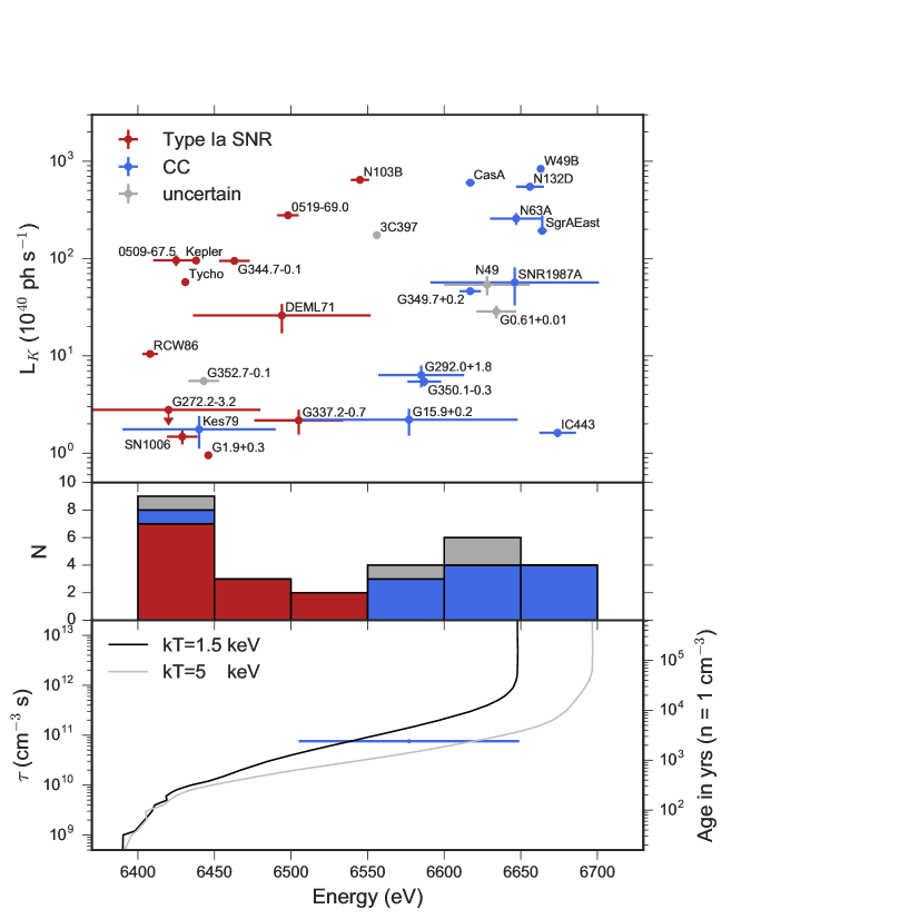
Figure 8: Top panel : Centroid energy and luminosity of Fe K lines detected in SNRs. The main sample and values obtained with Suzaku are taken from Yamaguchi et al. (2014), augmented with XMM-Newton results for DEM L71 (Maggi et al. 2016) and SNR G15.9+0.2 (this work), and Suzaku observations of Kes 79 (Sato et al. 2016) and SNR G272.2$-$3.2 (Kamitsukasa et al. 2016). For the latter, only an upper limit is shown since the distance is poorly constrained (2 to 10 kpc, e.g. Harrus et al. 2001). Objects in red and blue are type Ia and CC SNRs, respectively. Those in grey are uncertain. Middle panel : Histogram showing the distribution of Fe K centroid energy in SNRs using the same colour code as above. Bottom panel : Expected centroid energy of the Fe K line in a vpshock model as function of $\tau$, for $kT=1.5$ keV (black) and 5 keV (grey). The best-fit $\tau$ and range of centroid energy of SNR G15.9+0.2 are indicated. The right-hand $y-$axis translates the ionisation timescale $\tau$ into an age, for a uniform ambient density of $n_{e}=1$ cm^-3.

Since there is strong evidence, as shown above, that SNR G15.9+0.2 originates in a core-collapse SN, a high centroid energy is expected for the Fe K line. Instead we found an intermediate value of 6577${}_{-70}^{+73}$ eV when following the same method as Yamaguchi et al. (i.e. one free-width Gaussian on the integrated SNR spectrum), making SNR G15.9+0.2 the CC SNR with the lowest Fe K centroid among the sample of Y14 (Fig. 8, top panel). The moderate spatial resolution enabled by the existing XMM-Newton data reveals that the Fe K emission is non-uniform: In the “Shell E” region, we detect both $\sim$6.4 keV and $\sim$6.65 keV signals attributable to contributions from pooly and highly ionised iron, which in the overall spectrum produce a line at the observed centroid of 6.58 keV.

The detection of a 6.4 keV line from a CC SNR is remarkable. Such a line has been found in CC SNRs Kes~79 (Sato et al. 2016) and HESS~J1745$-$303 (Bamba et al. 2009), but it was proposed not to be of ionised plasma origin. In Kes 79, the 6.4 keV emission is attributed to K-shell ionisation of neutral iron by the interaction of locally accelerated protons with a nearby molecular cloud, while Bamba et al. (2009) suggested that the line in HESS J1745$-$303 was from an X-ray reflection nebula reflecting X-rays from previous Galactic centre activity off a molecular cloud. Neither of these scenarios are likely for SNR G15.9+0.2: There are no striking spatial correlations of the 6.4 keV emission with molecular clouds as in Kes 79 (see Fig. 9), nor reported detection of OH maser to support an interaction with molecular clouds (Green et al. 1997). An X-ray reflection nebula origin, as in HESS J1745$-$303, is also not favoured given the lack of a suitable nearby hard X-ray source, and the poor spatial correlation between the 6.4 keV emission and molecular material.

In SNR G15.9+0.2, an ionised plasma origin is favoured. The variations in ionisation between east and west regions, and inner/outer parts of “Shell E” (Sect. 3.2.2) points to a range of $n_{e}t$ due to variations in the ambient density encountered by the shock, or to different times since the plasma was shocked. The material in the east could be part of a cavity that the shock encountered recently, akin to the case in the type Ia SNR RCW~86 (Broersen et al. 2014). Such density variations and/or cavities are likely to be common, especially around young CC SNRs, but are hard to observe, except in the brightest and more extended sources. As another instance, Safi-Harb et al. (2005) found different Fe K centroids in eastern and western regions of 3C 397, attributed to density gradients.

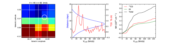
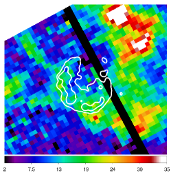
Figure 9: Left : ¹²CO spectrum at the position of the source (red) with corresponding kinematic distance (blue). Middle : H I, ¹²CO, and total column densities towards SNR G15.9+0.2 as a function of $V_{\rm LSR}$. Right : ¹³CO intensity map in the velocity range 18 km s^-1 ¡ $V_{\rm LSR}$ ¡ 32 km s^-1, in units of K km s^-1. X-ray contours are overlaid in white. The black stripe comes from bad columns which have been set to 0.

Patnaude et al. (2015) have modelled CC SNe exploding in CSM modified by progenitors’ winds and followed their dynamics (i.e. shock radius) and spectral evolution of Fe K emission (centroid and luminosity). Although these models were able to reproduce the higher centroids (above 6550 eV) observed in CC SNRs, there were many outliers where either the correct shock radius and centroid were not reproduced by the models, or where the Fe K luminosity was severely underpredicted. Placing SNR G15.9+0.2 in that context, the bulk Fe K properties (in particular its low centroid) and size of about 4 ($D$ / 5 kpc) pc (see Sect. 3.1) can be reproduced by their SN 1987A or SN~1993J models (e.g. Fig. 2, Patnaude et al. 2015). The low Fe K luminosity of SNR G15.9+0.2 ($\sim 2\times 10^{40}$ ($D$ / 5 kpc) photon s^-1) can be reproduced by most of their models in the lower mass loss rate/higher wind velocity cases.

Regardless of type, the distribution of Fe K centroids in SNRs is peaked at the low- and high-energy ends (see Fig. 8, middle panel) with relatively few objects between 6.5 keV and 6.6 keV. This is due to the rapid transition between a roughly 6.4 keV centroid (no iron above the Fe XVII state) and a 6.6$-$6.7 keV centroid (most iron above Fe XX). To illustrate this, we simulated emission from a pure-iron ionising plasma (vpshock in XSPEC) at $kT=1.5$ keV and 5 keV, with $\tau$ between 10⁸ s cm^-3 and $5\times 10^{13}$ s cm^-3. Fake spectra were produced using the EPIC-pn response and analysed in the same fashion as in Y14 and in this work. The curves of the expected centroids are shown in the bottom panel of Fig. 8. The Fe K transition occurs briefly, or more specifically over a small $\tau$ interval, between a few 10¹⁰ s cm^-3 and a few 10¹¹ s cm^-3. For SNRs expanding in a constant ambient density of $n_{e}=1$ cm^-3, this happens at an age of $\sim 1000-5000$ yr. The oldest type Ia SNRs in the sample of Y14 are from 4500 to 6000 yr old (SNR G337.2$-$0.7 and SNR G344.7$-$0.1). They are associated with relatively low density ($n_{e}\sim$ 0.3 to 0.8 cm^-3, Rakowski et al. 2006; Giacani et al. 2011) so that a low Fe ionisation is expected even at this age.

The possibility remains open for a type Ia SNR in a denser medium ($\gtrsim 2$ cm^-3) to reach a high ionisation of iron within a few thousand years and populate the Fe K centroid region dominated so far by CC SNRs. Without definitive evidence as to its type (Park et al. 2012), N49 might be such an object, since it is interacting with a relatively high density (at least 2–25 cm^-3, Sankrit et al. 2004; Dopita et al. 2016). Symmetrically, it can not excluded that some CC SNRs are found at the low ionisation end. Part of SNR G15.9+0.2, for instance, still has emission at 6.4 keV, while SNR~G352.7$-$0.1 has an Fe K centroid at 6.44 keV and is also of uncertain type; some studies suggest that it is the remnant a CC SNR (Giacani et al. 2009; Pannuti et al. 2014). Another caveat is that the current sample of Fe K emitting objects inherently contains some age bias, the youngest objects being preeminently of type Ia. There are six type Ia SNRs younger than $\sim 1000$ yr, but only three CC SNRs below the 2000 yr mark. Together with the lower density expected around type Ia SN progenitors, this bias contributes to separate the Fe K centroids of both classes. We conclude that the Fe K centroid-luminosity diagram provides valuable information about an SNR, but care should be taken when using it as a typing tool without any knowledge of the surrounding medium or indication of age. This is particularly true for unresolved objects, e.g. young SNRs in external galaxies, or objects where the nature of the Fe K emission is unknown and might not be from an ionised plasma, as is the case in Kes 79 and HESS J1745$-$303.

4.3 Constraining the age of and distance to SNR G15.9+0.2

To constrain the distance to the SNR, we compared the absorption along the line of sight derived from the X-ray and from H I and ¹²CO (1-0) observations. Figure 9 (left panel) shows the velocity spectra at the SNR centre (RA = 18^h 18^m 53.8^s, DEC = $-$15° 01^m 38^s) integrated within a radius of 3′. The ¹²CO observations are from the CfA survey (Dame et al. 2001) and the H I data from the SGPS survey (Haverkorn et al. 2006). The corresponding kinematic distances assuming the circular Galactic rotation model of Hou et al. (2009) with a distance to the Galactic center of 8 kpc are also shown. We note that the bulk of the material along the line of sight is at radial velocities relative to the local standard of rest (LSR) of $V_{\rm LSR}$ ¡ 60 km s^-1 which is equivalent to a lower limit on the distance of 5 kpc. The cumulative $N_{\rm H}$ derived from H I and ¹²CO as a function of $V_{\rm LSR}$ is shown in Fig. 9 (middle panel) where all the material is assumed to be at the near distance allowed by the Galactic rotation curve, providing therefore a lower limit on the distance. The CO-to-H₂ mass conversion factor and the H I brightness temperature to column density used is respectively of $1.8\times 10^{20}$ cm^-2 K^-1 km^-1 s (Dame et al. 2001) and $1.82\times 10^{18}$ cm^-2 K^-1 km^-1 s (Dickey & Lockman 1990).

Most of the absorption along the line of sight is due to the structures at $V_{\rm LSR}$ ¡ 60 km s^-1, representing an integrated $N_{\rm H}=2.2\times 10^{22}$ cm^-2. With an X-ray absorption value of $4.58\pm 0.11\times 10^{22}$ cm^-2 (see Table 3), we argue that the SNR is behind these structures and set a strict lower limit to its distance at 5 kpc. This is consistent with the results of a carbon atmosphere fit to the CCO emission (Klochkov et al. 2016) that yields a large distance (although highly uncertain) of 10${}^{+9}_{-5}$ kpc.

However, the total $N_{\rm H}$ integrated along the entire velocity range derived from H I and ¹²CO amounts to $\sim 3.5\times 10^{22}$ cm^-2, still significantly less than the X-ray value. This discrepancy could be due to an inadequate value of the CO-to-H₂ mass conversion factor which can vary within the Galaxy (e.g. Remy et al. 2015) or missing material not traced by HI or ¹²CO emission. In particular in dense molecular clouds, the core of the cloud is not well traced by ¹²CO owing to saturation of the emission.

The ¹³CO (1-0) line emission provides a tracer to investigate the core of the dense molecular clouds. In Fig. 9 (right panel), we show the high-resolution ¹³CO intensity map from the GRS survey (Jackson et al. 2006). This map was obtained by integrating velocities between 18 km s^-1 ¡ $V_{\rm LSR}$ ¡ 32 km s^-1 corresponding to main peak of ¹³CO emission located at the same velocity as the brightest ¹²CO peak shown in Fig. 9. This material is likely in the foreground of the SNR. Small clouds are seen at the position of the shell E and shell SW regions, explaining the spatial variations of $N_{H}$ found in Sect. 3.2.1.

To investigate the age of the SNR in more detail, we used the equations describing the evolution of the forward shock $R$ presented by Truelove & McKee (1999) and generalised to a steady stellar wind environment with $\rho(r)\propto r^{-2}$ by Laming & Hwang (2003) & Hwang & Laming (2012). We fixed the explosion energy to $E=10^{51}$ ergs, $n=9$, and $s=2$, where $n$, and $s$ are the ejecta and ambient medium density profile ($\rho(r)\propto r^{-n,s}$). The ejecta mass was fixed to 14 $M_{\sun}$ (for an initial progenitor mass of 25 $M_{\sun}$) according to mass budget models of core-collapse supernovae by Sukhbold et al. (2016).

The ambient medium density is derived from the X-ray thermal emission of the “faint NW”, the least affected by ejecta and therefore best representing shocked ISM. The normalisation of the fiducial model in that region (Table 3) is proportional to the volume emission measure $\int n_{e}n_{H}dV$, which can be linked to the pre-shock ambient hydrogen density $n_{\mathrm{H,}0}$ assuming a Sedov profile (e.g. Maggi et al. 2014, Eq. 1). With the uncertainties on the normalisation in the “faint NW” region, we measure a range of $n_{\mathrm{H,}0}=(0.36-0.70)$ ($D$ / 5 kpc)^-1/2 cm^-3.

Considering the lower limit on the distance of 5 kpc derived above, we obtain a lower limit on the age of 2 kyr. This reproduces the observed angular distance (3.7′) between the CCO and the tip of the faint NW region (Fig. 2). If the SNR is near the Galactic centre, at a distance of 8.5 kpc as assumed by R06, the age estimate is $\sim$ (4.5–6) kyr. In the case where the shock has evolved only a small fraction of its lifetime in the steep wind profile, and quickly after evolved in the uniform shocked wind region (assuming therefore $s=0$), the corresponding ages are $t_{SNR}>$ 1.6 kyr and $t\sim(3.5-4)$ kyr for a distance of 5 and 8.5 kpc, respectively.

4.4 Expansion of SNR G15.9+0.2

PRELIM: Non-uniform expansion? Relation to CCO (geometric centre different from explosion site, preventing an estimate of pulsar SN kick).

5 Summary

We have studied the Galactic SNR G15.9+0.2, observed serendipitously with XMM-Newton. The remnant exhibits a shell morphology with the brightest regions in the east and south-west, and the faintest and softest to the north-west. Elemental abundances, particularly in the bright regions, are markedly supersolar, betraying a SN ejecta origin. Analysis of the ejecta abundance pattern establishes SNR G15.9+0.2 as a core-collapse SNR and suggests a progenitor mass of 20–25 $M_{\sun}$. This makes the physical association with the CCO CXOU J181852.0$-$150213 detected in its interior very likely.

We report for the first time detection of Fe K emission from SNR G15.9+0.2, using a careful treatment of all background components to ensure that this signal is genuinely from the SNR. We detect signal at both the low (6.4 keV) and high (6.67 keV) ionisation end of the line, with spatial variation across the SNR. Because SNR G15.9+0.2 is the core-collapse SNR with the lowest overall Fe K centroid energy, caution should be used when typing SNRs based on this criterion alone.

Matching the X-ray $N_{H}$ to atomic and molecular gas structures along the line of sight, we set a conservative limit of 5 kpc for the distance towards the source. At such distances and for a reasonable set of parameters affecting the remnant’s dynamics, we constrain its age to be likely more than 2000 yr.