Lattice calculation of the pion transition form factor $\pi^{0}\to\gamma^{*}\gamma^{*}$

Abstract:

We calculate the pion transition form factor ${\cal F}_{\pi^{0}\gamma^{*}\gamma^{*}}(q_{1}^{2},q_{2}^{2})$, which describe the interaction of an on-shell pion with two off-shell photons, using lattice QCD simulations with two degenerate flavors of dynamical quarks. This form factor is the main ingredient in the calculation of the pion-pole contribution to hadronic light-by-light scattering in the muon $g-2$, $a_{\mu}^{\mathrm{HLbL};\pi^{0}}$. We focus our study on the spacelike region with photon virtualities up to $1.5~{}\mathrm{GeV}^{2}$, not yet measured experimentally. Several lattice spacings and pion masses are used to extrapolate the results to the physical point and a comparison with different phenomenological models is performed. Finally, we use our extrapolated form factor to provide a lattice determination of $a_{\mu}^{\mathrm{HLbL};\pi^{0}}$.

1 Introduction

The anomalous magnetic moment of the muon provides one of the most precise tests of the Standard Model of particle physics [1, 2] and a persistent discrepancy of about $3-4$ standard deviations [3] exists between experiment and theory. In the near future, the experimental error is expected to be reduced by a factor four [4]. The theoretical error is now dominated by hadronic contributions : the hadronic vacuum polarization (HVP) and hadronic light-by-light scattering (HLbL) and, for the latter, no reliable estimate exists yet and systematic errors are difficult to estimate. However, recently a dispersive approach was proposed [5] which relates the numerically dominant pseudoscalar-pole contribution, and the pion-loop in HLbL with on-shell intermediate pseudoscalar states to measurable form factors and cross-sections with off-shell photons: $\gamma^{*}\gamma^{*}\to\pi^{0},\eta,\eta^{\prime}$ and $\gamma^{*}\gamma^{*}\to\pi^{+}\pi^{-},\pi^{0}\pi^{0}$. Within this framework, the pion-pole contribution is obtained by integrating some weight functions times the product of a single-virtual and a double-virtual transition form factors for spacelike momenta [1]. In particular, the weight functions turn out to be peaked at low momenta such that the main contribution to $a_{\mu}^{{\rm HLbL};\pi^{0}}$ arises from photon virtualities below $1~{}\mathrm{GeV}^{2}$ [6], a kinematical range accessible on the lattice. From the experimental point of view, only the single-virtual form factor for the pion ${\cal F}_{\pi^{0}\gamma^{*}\gamma^{*}}(-Q^{2},0)$ has been measured [7] in the spacelike region $Q^{2}\in[0.5,40]~{}\mathrm{GeV}^{2}$. From the theoretical point of view, the form factor is constrained by the Adler-Bell-Jackiw (ABJ) anomaly in the chiral limit such that ${\cal F}_{\pi^{0}\gamma^{*}\gamma^{*}}(0,0)=1/(4\pi^{2}F_{\pi})$ [8]. The single-virtual form factor has been computed in the framework of factorization in QCD (operator-product expansion (OPE) on the light-cone) and one finds the Brodsky-Lepage behavior [9]

$${\cal F}_{\pi^{0}\gamma^{*}\gamma^{*}}(-Q^{2},0)\xrightarrow[Q^{2}\to\infty]{}2F_{\pi}/Q^{2}\,.$$ (1)

Finally, the double-virtual form factor where both momenta become simultaneously large has been computed using the OPE at short distances. In the chiral limit the result reads [10, 11]

$$\vspace{-0.2cm}{\cal F}_{\pi^{0}\gamma^{*}\gamma^{*}}(-Q^{2},-Q^{2})\xrightarrow[Q^{2}\to\infty]{}2F_{\pi}/(3Q^{2})\,.$$ (2)

Therefore, the double-virtual form factor in the kinematical range of interest $[0-1]~{}\mathrm{GeV}^{2}$ for the computation of the HLbL contribution to the muon $g-2$ is still unknown and the available estimates rely on phenomenological models [1, 12]. Previous lattice studies [13] ¡ on the decay $\pi^{0}\to\gamma\gamma$ (form factor at very low momenta). More details on this work can be found in [14].

2 Methodology

In Minkowski spacetime, the form factor of interest is defined via the following matrix element

$$\vspace{-0.2cm}M_{\mu\nu}(p,q_{1})=i\int\mathrm{d}^{4}x\,e^{iq_{1}x}\,\langle\Omega|T\{J_{\mu}(x)J_{\nu}(0)\}|\pi^{0}(p)\rangle=\epsilon_{\mu\nu\alpha\beta}\,q_{1}^{\alpha}\,q_{2}^{\beta}\,{\cal F}_{\pi^{0}\gamma^{*}\gamma^{*}}(q_{1}^{2},q_{2}^{2})\,,$$ (3)

where $q_{1}$ and $q_{2}$ are the photon momenta and $p=q_{1}+q_{2}$ is the on-shell pion momentum. $J_{\mu}=\sum_{f}Q_{f}\,\overline{\psi}_{f}\gamma_{\mu}\psi_{f}$ is the hadronic component of the electromagnetic current and we use the relativistic normalization of states $\langle\pi^{0}(p)|\pi^{0}(p^{\prime})\rangle=(2\pi)^{3}\,2E_{\pi}(\vec{p})\ \delta^{(3)}(\vec{p}-\vec{p}^{\ \prime})$. To compute the form factor on the lattice, we follow the method introduced in [15]. Keeping $q_{1,2}^{2}<M^{2}_{V}={\rm min}(M^{2}_{\rho},4m_{\pi}^{2})$, one can show [16] that the matrix element in Euclidean spacetime is

$$M_{\mu\nu}=(i^{n_{0}})M_{\mu\nu}^{\rm E},\quad M_{\mu\nu}^{\rm E}\equiv-\int\mathrm{d}\tau\,e^{\omega_{1}\tau}\int\mathrm{d}^{3}z\,e^{-i\vec{q}_{1}\vec{z}}\,\langle 0|T\left\{J_{\mu}(\vec{z},\tau)J_{\nu}(\vec{0},0)\right\}|\pi(p)\rangle\,,$$ (4)

where $\omega_{1}$ is a real free parameter such that $q_{1}=(\omega_{1},\vec{q}_{1})$ and $n_{0}$ denotes the number of temporal indices carried by the two vector currents. Therefore, one is led to consider the following three-point correlation function on the lattice

$$C^{(3)}_{\mu\nu}(\tau,t_{\pi})=a^{6}\sum_{\vec{x},\vec{z}}\,\big{\langle}T\left\{J_{\mu}(\vec{z},t_{i})J_{\nu}(\vec{0},t_{f})P^{{\dagger}}(\vec{x},t_{0})\right\}\big{\rangle}\,e^{i\vec{p}\,\vec{x}}\,e^{-i\vec{q}_{1}\vec{z}}\,,$$ (5)

where $\tau=t_{i}-t_{f}$ is the time separation between the two vector currents and $t_{\pi}={\rm min}(t_{f}-t_{0},t_{i}-t_{0})$. The matrix element with on-shell pion is obtained by considering the large $t_{\pi}$ limit. By defining

$$A_{\mu\nu}(\tau)=\lim_{t_{\pi}\rightarrow+\infty}C^{(3)}_{\mu\nu}(\tau,t_{\pi})\,e^{E_{\pi}t_{\pi}}\,,\quad\widetilde{A}_{\mu\nu}(\tau)=\left\{\begin{array}[]{l@{~~~}l}A_{\mu\nu}(\tau)\hfil~{}~{}~{}&\tau>0\\ A_{\mu\nu}(\tau)\,e^{-E_{\pi}\tau}\hfil~{}~{}~{}&\tau<0\end{array}\right.\;,$$ (6)

and using Eq. (4), $M_{\mu\nu}$ can be obtained via

$$M_{\mu\nu}^{\rm E}=\frac{2E_{\pi}}{Z_{\pi}}\left(\int_{-\infty}^{0}\,\mathrm{d}\tau\,e^{\omega_{1}\tau}\,A_{\mu\nu}(\tau)\,e^{-E_{\pi}\tau}+\int_{0}^{\infty}\,\mathrm{d}\tau\,e^{\omega_{1}\tau}\,A_{\mu\nu}(\tau)\right)=\frac{2E_{\pi}}{Z_{\pi}}\int_{-\infty}^{\infty}\,\mathrm{d}\tau\,e^{\omega_{1}\tau}\,\widetilde{A}_{\mu\nu}(\tau)\,,$$ (7)

where the overlap factor $Z_{\pi}$ and the pion energy can be extracted from the asymptotic behavior of the two-point pseudoscalar correlation function.

3 Lattice computation

This work is based on a subset of the $n_{f}=2$ CLS (Coordinated Lattice Simulations) ensembles generated using the nonperturbatively $\mathcal{O}(a)$-improved Wilson-Clover action for fermions and the plaquette gauge action for gluons. As shown in Table 1, three lattice spacings in the range [0.05-0.075] fm are considered with pion masses down to 193 MeV and $Lm_{\pi}>4$ such that volume effects are expected to be negligible [17]. For more details on the ensembles, see [19]. The connected part of the three-point correlation function in Eq. (5) has been computing using one ‘local’ vector current $J_{\mu}^{l}(x)=\sum_{f}Q_{f}\ \overline{\psi}_{f}(x)\gamma_{\mu}\psi_{f}(x)$ and one ‘point-split’ vector current

$$J_{\mu}^{c}(x)=\sum_{f}\frac{Q_{f}}{2}\left(\overline{\psi}_{f}(x+a\hat{\mu})(1+\gamma_{\mu})U^{{\dagger}}_{\mu}(x)\psi_{f}(x)-\overline{\psi}_{f}(x)(1-\gamma_{\mu})U_{\mu}(x)\psi_{f}(x+a\hat{\mu})\right)\,,$$ (8)

whereas the disconnected part is computed using two local vector currents. In the $\mathcal{O}(a)$-improved theory, the renormalized currents read $J_{\mu}^{\alpha,R}(x)=Z^{\alpha}_{V}(1+b_{V}^{\alpha}(g_{0})am_{q})\left(J_{\mu}^{\alpha}(x)+ac_{V}^{\alpha}\partial_{\nu}T_{\mu\nu}\right)$ with $\alpha=(\rm{local},\rm{conserved})$ and where $b_{V}^{\alpha}$ and $c_{V}^{\alpha}$ are improvement coefficients. The point-split vector current satisfies the Ward identity and does not need any renormalization factor: $Z_{V}^{c,I}=1$, $b_{V}^{c,I}=0$ whereas $Z_{V}^{l}$ has been computed non-perturbatively in [18, 19]. We neglect the contribution from the tensor density $T_{\mu\nu}(x)$ such that $\mathcal{O}(a)$-improvement is only partially implemented. We choose the pion reference frame, $\vec{p}=0$, where both photons have back-to-back spatial momenta ($\vec{q}_{2}=-\vec{q}_{1}$) and the kinematical range accessible on the lattice can be parametrized by

$$q_{1}^{2}=\omega_{1}^{2}-\vec{q}_{1}^{\,2}\,,\quad q_{2}^{2}=(m_{\pi}-\omega_{1})^{2}-\vec{q}_{1}^{\,2}\,.$$

We consider multiple values of $\vec{q}_{1}$ to obtain virtualities up to $|q_{1,2}^{2}|\approx 1.5~{}\mathrm{GeV}^{2}$ as can be seen in Fig. 1. In this kinematical setup and using the Lorentz structure of the form factor one can show that only the spatial components are non-zero and can be written

$$A_{kl}(\tau)=-iq_{kl}\,A(\tau)\,,\qquad q_{kl}\equiv\epsilon_{kl\alpha\beta}\,q_{1}^{\alpha}\,q_{2}^{\beta}=m_{\pi}\,\epsilon_{kli}\,q_{1}^{i}\,,$$ (9)

where $A(\tau)$ is a scalar under the spatial rotation group ($\widetilde{A}(\tau)$ is defined in the same way).

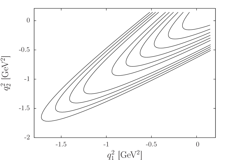
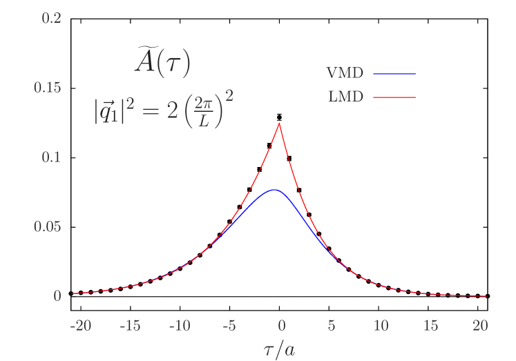
Figure 1: (left) Kinematic reach in the photon virtualities ($q_{1}^{2},q_{2}^{2}$) in our setup with the pion at rest, for the lattice resolution $48^{3}\times 96$ at $a=0.065\,{\rm fm}$. (Right) The function $\widetilde{A}(\tau)$ (black points) and the VMD (blue line) and LMD (red line) fits used to describe the tail of the function at large $\tau$ for the lattice ensemble F7.

Table 1: Parameters of the simulations: the bare coupling $\beta=6/g_{0}^{2}$, the lattice resolution, the hopping parameter $\kappa$, the lattice spacing $a$ in physical units extracted from [19].

CLS	$\quad\beta\quad$	$L^{3}\times T$	$\kappa$	$a~{}(\mathrm{fm})$	$m_{\pi}~{}(\mathrm{MeV})$	$F_{\pi}~{}(\mathrm{MeV})$	$m_{\pi}L$	$\#$confs
A5	$5.2$	$32^{3}\times 64$	$0.13594$	$0.0749(8)$	$334(4)$	$106.0(6)$	4.0	400
B6		$48^{3}\times 96$	$0.13597$		$281(3)$	$102.3(5)$	5.2	400
E5	$5.3$	$32^{3}\times 64$	$0.13625$	$0.0652(6)$	$437(4)$	$115.2(6)$	4.7	400
F6		$48^{3}\times 96$	$0.13635$		$314(3)$	$105.3(6)$	5.0	300
F7		$48^{3}\times 96$	$0.13638$		$270(3)$	$100.9(4)$	4.3	350
G8		$64^{3}\times 128$	$0.136417$		$194(2)$	$95.8(4)$	4.1	300
N6	$5.5$	$48^{3}\times 96$	$0.13667$	$0.0483(4)$	$342(3)$	$105.8(5)$	4.0	450
O7		$64^{3}\times 128$	$0.13671$		$268(3)$	$101.2(4)$	4.2	150

4 Results

4.1 Extraction of the form factor

In Eq. (7), the time integration is performed using numerical data up to $\tau_{c}\approx 1.3~{}\mathrm{fm}$. For $\tau>\tau_{c}$, the contribution of the tail is estimated from a fit of our data with the analytical expression of $A^{\mathrm{VMD}}_{kl}(\tau)$ in the vector meson dominance model (VMD), derived in [14] (see the next subsection for a description of the models). A typical fit for the lattice ensemble F7 is depicted in the right panel of Fig. 1 where the result using the lowest meson dominance model (LMD) [20] rather that the VMD is also shown. Finally, the disconnected contribution to the three-point correlation function has been computed for the lattice ensemble E5 and only for the first three values of the spatial momentum $|\vec{q}_{1}|^{2}=n^{2}(2\pi/L)^{2}$, $n^{2}=1,2,3$. It contributes to less than $1\%$ of the total contribution and we conclude that the disconnected contribution is negligible at our level of accuracy.

4.2 Fits in four-momentum space

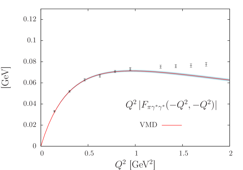
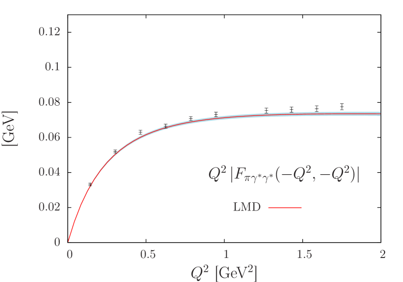
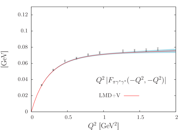
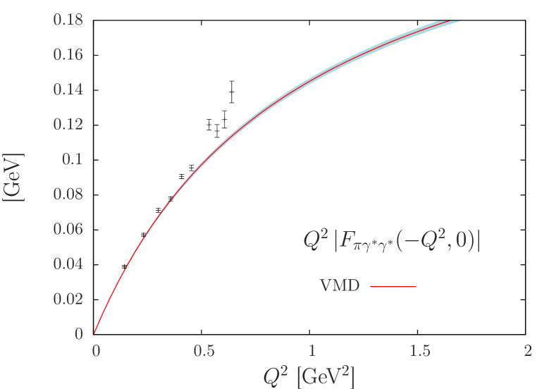
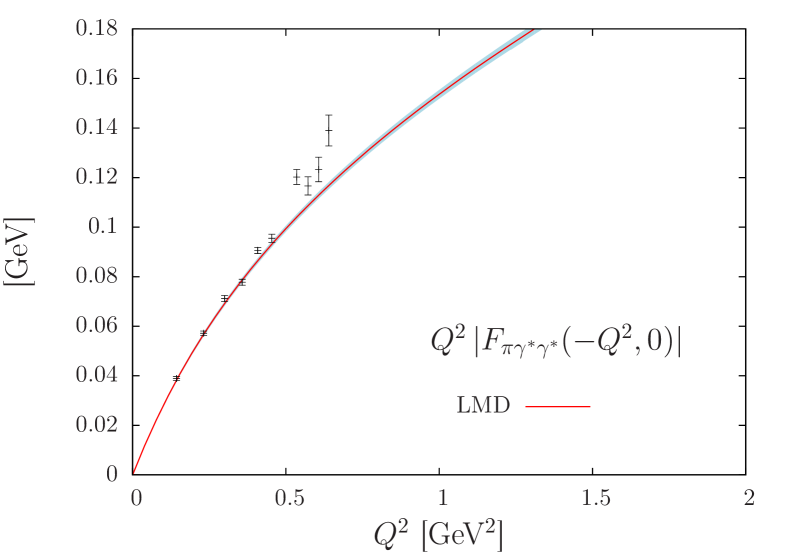
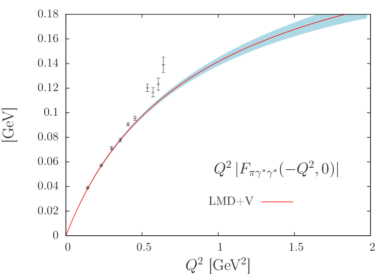
Figure 2: Comparison of the VMD, LMD and LMD+V fits for the lattice ensemble O7. The red line corresponds to the results from our global fit. The VMD model falls-off as ${\cal F}_{\pi^{0}\gamma^{*}\gamma^{*}}^{\rm VMD}(-Q^{2},-Q^{2})\sim 1/Q^{4}$ in the double virtual case and fails to describe the numerical data. Note that points at different $Q^{2}$ are correlated.

We first compare our results with the VMD model, parametrized by

$${\cal F}_{\pi^{0}\gamma^{*}\gamma^{*}}^{\mathrm{VMD}}(q_{1}^{2},q_{2}^{2})=\frac{\alpha M_{V}^{4}}{(M_{V}^{2}-q_{1}^{2})(M_{V}^{2}-q_{2}^{2})}\,.$$ (10)

Using $\alpha=1/(4\pi^{2}F_{\pi})=0.274~{}\mathrm{GeV}^{-1}$, it reproduces the anomaly constraint in the chiral limit. This model is also compatible with the Brodsky-Lepage behavior (1) in the single-virtual case but falls off faster than the OPE prediction (2) in the double-virtual case. To reduce the number of fit parameters, a global fit is performed where all lattice ensembles are fitted simultaneously assuming a linear dependence in both $a/a_{\beta=5.3}$ and $\widetilde{y}=m^{2}_{\pi}/8\pi^{2}F^{2}_{\pi}$ for each parameter of the model. We obtain at the physical point

$$\alpha^{\mathrm{VMD}}=0.243(18)~{}\mathrm{GeV}^{-1}\,,\quad M_{V}^{\mathrm{VMD}}=0.944(34)~{}\mathrm{GeV}\,.$$ (11)

As can be seen in Fig. 2, the VMD model leads to a poor description of our data ($\chi^{2}/\mathrm{d.o.f.}=2.9$, uncorrelated fit), especially in the double virtual case and at large Euclidean momenta. The second model, the LMD model [20], can be parametrized as

$${\cal F}_{\pi^{0}\gamma^{*}\gamma^{*}}^{\mathrm{LMD}}(q_{1}^{2},q_{2}^{2})=\frac{\alpha M_{V}^{4}+\beta(q_{1}^{2}+q_{2}^{2})}{(M_{V}^{2}-q_{1}^{2})(M_{V}^{2}-q_{2}^{2})}\,.$$ (12)

Again, this model reproduces the anomaly constraint and is now compatible with the OPE asymptotic behaviour where $\beta=-F_{\pi}/3$ is the theoretical preferred estimate (see Eq. 2). However, this model does not reproduce the Brodsky-Lepage behavior for the single-virtual form factor given in Eq. (1). Using $\alpha$, $\beta$ and $M_{V}$ as free parameters, we now obtain

$$\alpha^{\mathrm{LMD}}=0.275(18)(3)~{}\mathrm{GeV}^{-1}\,,\quad\beta=-0.028(4)(1)~{}\mathrm{GeV}\,,\quad M_{V}^{\mathrm{LMD}}=0.705(24)(21)~{}\mathrm{GeV}\,,$$ (13)

with $\chi^{2}/\mathrm{d.o.f.}=1.3$ (uncorrelated fit) (Fig. 2). The first error is statistical and the second error include systematics as discussed in [14]. Although this model fails to reproduce the Brodsky-Lepage behavior, it gives a good description of our data in the considered kinematical range. The anomaly is recovered with a statistical error of 7% and $\beta$ is compatible with the OPE asymptotic result given in Eq. (2). Finally, the LMD+V model, proposed in Ref. [21], includes a second vector resonance and can be parametrized by

$${\cal F}_{\pi^{0}\gamma^{*}\gamma^{*}}^{\mathrm{LMD+V}}(q_{1}^{2},q_{2}^{2})=\frac{\widetilde{h}_{0}\,q_{1}^{2}q_{2}^{2}(q_{1}^{2}+q_{2}^{2})+\widetilde{h}_{1}(q_{1}^{2}+q_{2}^{2})^{2}+\widetilde{h}_{2}\,q_{1}^{2}q_{2}^{2}+\widetilde{h}_{5}\,M_{V_{1}}^{2}M_{V_{2}}^{2}\,(q_{1}^{2}+q_{2}^{2})+\alpha\,M_{V_{1}}^{4}M_{V_{2}}^{4}}{(M_{V_{1}}^{2}-q_{1}^{2})(M_{V_{2}}^{2}-q_{1}^{2})(M_{V_{1}}^{2}-q_{2}^{2})(M_{V_{2}}^{2}-q_{2}^{2})}\,.$$ (14)

One main advantage of this model is that it fulfils all the theoretical constraints discussed in Sec. 1 if one sets $\widetilde{h}_{1}=0$ (which is explicitly done in our fits) and $\widetilde{h}_{0}=-F_{\pi}/3$. In Ref. [21], the masses are set to their physical values $M_{V_{1}}=m^{\exp}_{\rho}=0.775~{}\mathrm{GeV}$ and $M_{V_{2}}=m^{\exp}_{{\rho}^{\prime}}=1.465~{}\mathrm{GeV}$. The parameter ${\widetilde{h}}_{2}=0.327~{}\mathrm{GeV}^{3}$ can be fixed by comparing with the subleading term in the OPE in Eq. (2) (Ref. [22, 11]) and the parameter ${\widetilde{h}}_{5}=-0.166(6)~{}\mathrm{GeV}$ has been determined in Ref. [21] by a fit to the CLEO data [7] for the single-virtual form factor.

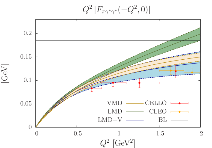
Figure 3: Lattice extrapolations for the VMD, LMD and LMD+V models. (left) Single-virtual form factor. (right) Double-virtual form factor at $Q_{1}^{2}=Q_{2}^{2}$.

To get stable fits, we enforce the constraint $M_{V_{1}}=m_{\rho}^{\exp}$ at the physical point but still allowing for chiral corrections. For $M_{V_{2}}$, inspired by quark models, we assume a constant shift in the spectrum and set $M_{V_{2}}(\widetilde{y})=m^{\exp}_{\rho^{\prime}}+M_{V_{1}}(\widetilde{y})-m^{\exp}_{\rho}$. Finally, we impose the theoretical constraint $\widetilde{h}_{0}=-F_{\pi}/3$ in the continuum and chiral limit but, again, still allowing for chiral and lattice artefacts corrections. Using these assumptions, we obtain

$$\alpha^{\mathrm{LMD+V}}=0.273(24)(7)~{}\mathrm{GeV}^{-1}\,,\ \widetilde{h}_{2}=0.345(167)(83)~{}\mathrm{GeV}^{3}\,,\ \widetilde{h}_{5}=-0.195(70)(34)~{}\mathrm{GeV}\,,$$ (15)

with $\chi^{2}/\mathrm{d.o.f.}=1.4$ (uncorrelated fit). This model also gives a good description of our data as can be seen in Fig. 2 and turns out to be close to the LMD model in the kinematical range considered here. The systematic error has been estimated by varying our assumptions on $M_{V_{1}}$ and $M_{V_{2}}$. Again, the anomaly constraint is recovered within statistical error bars and the values of $\widetilde{h}_{2}$ and $\widetilde{h}_{5}$ are in good agreement with phenomenology.

The form factor extrapolated to the physical point for each model is shown in Fig. 3. In the single-virtual case, the VMD and LMD+V models are in good agreement with the experimental data whereas the LMD model starts to deviate at $Q^{2}=1~{}\mathrm{GeV}^{2}$. In the double-virtual case, the LMD and LMD+V models are similar and already close to their asymptotic behavior at $Q^{2}\sim 1.5~{}\mathrm{GeV}^{2}$ where we have lattice data. Finally, using the formalism developed in Ref. [1] and our result for the form factor, we estimate the pion-pole contribution $a_{\mu}^{\mathrm{HLbL};\pi^{0}}$ to hadronic light-by-light scattering in the muon $g-2$. Our preferred estimate for $a_{\mu}^{\mathrm{HLbL};\pi^{0}}$ is obtained with the fitted LMD+V model [14],

$$a_{\mu;\mathrm{LMD+V}}^{\mathrm{HLbL};\pi^{0}}=(65.0\pm 8.3)\times 10^{-11}\,.$$ (16)

For comparison, most model calculations yield results in the range $a_{\mu}^{\mathrm{HLbL};\pi^{0}}=(50-80)\times 10^{-11}$ with rather arbitrary, model-dependent error estimates, see Refs. [1, 12, 6] and references therein.

- [1] F. Jegerlehner and A. Nyffeler, Phys. Rept. 477, 1 (2009).
- [2] J. P. Miller, E. de Rafael, B. L. Roberts and D. Stöckinger, Ann. Rev. Nucl. Part. Sci. 62, 237 (2012).
- [3] K. A. Olive et al. [Particle Data Group Collaboration], Chin. Phys. C 38, 090001 (2014).
- [4] D. W. Hertzog, EPJ Web Conf. 118, 01015 (2016).
- [5] G. Colangelo, M. Hoferichter, M. Procura and P. Stoffer, JHEP 1409, 091 (2014); G. Colangelo, M. Hoferichter, B. Kubis, M. Procura and P. Stoffer, Phys. Lett. B 738, 6 (2014); G. Colangelo, M. Hoferichter, M. Procura and P. Stoffer, JHEP 1509, 074 (2015); V. Pauk and M. Vanderhaeghen, arXiv:1403.7503 [hep-ph]; V. Pauk and M. Vanderhaeghen, Phys. Rev. D 90, 113012 (2014).
- [6] M. Knecht and A. Nyffeler, Phys. Rev. D 65, 073034 (2002); A. Nyffeler, Phys. Rev. D 94, 053006 (2016).
- [7] H. J. Behrend et al. [CELLO Collaboration], Z. Phys. C 49, 401 (1991); J. Gronberg et al. [CLEO Collaboration], Phys. Rev. D 57, 33 (1998); B. Aubert et al. [BaBar Collaboration], Phys. Rev. D 80, 052002 (2009); S. Uehara et al. [Belle Collaboration], Phys. Rev. D 86, 092007 (2012).
- [8] S. L. Adler, Phys. Rev. 177, 2426 (1969); J. S. Bell and R. Jackiw, Nuovo Cim. A 60, 47 (1969).
- [9] G. P. Lepage and S. J. Brodsky, Phys. Lett. B 87, 359 (1979).
- [10] V. A. Nesterenko and A. V. Radyushkin, Sov. J. Nucl. Phys. 38, 284 (1983) [Yad. Fiz. 38, 476 (1983)].
- [11] V. A. Novikov et al., Nucl. Phys. B 237, 525 (1984).
- [12] J. Bijnens, EPJ Web Conf. 118, 01002 (2016).
- [13] H. W. Lin and S. D. Cohen, PoS ConfinementX , 113 (2012); X. Feng, S. Aoki, H. Fukaya, S. Hashimoto, T. Kaneko, J. i. Noaki and E. Shintani, Phys. Rev. Lett. 109, 182001 (2012).
- [14] A. Gérardin, H. B. Meyer and A. Nyffeler, Phys. Rev. D 94, 074507 (2016).
- [15] X. d. Ji and C. w. Jung, Phys. Rev. Lett. 86, 208 (2001); X. d. Ji and C. w. Jung, Phys. Rev. D 64 (2001) 034506; J. J. Dudek and R. G. Edwards, Phys. Rev. Lett. 97, 172001 (2006).
- [16] X. Feng et al., Phys. Rev. Lett. 109, 182001 (2012).
- [17] H. B. Meyer, Eur. Phys. J. A 49, 84 (2013).
- [18] M. Della Morte, R. Hoffmann, F. Knechtli, R. Sommer and U. Wolff, JHEP 0507, 007 (2005).
- [19] P. Fritzsch et al., Nucl. Phys. B 865, 397 (2012).
- [20] B. Moussallam, Phys. Rev. D 51, 4939 (1995); M. Knecht, S. Peris, M. Perrottet and E. de Rafael, Phys. Rev. Lett. 83, 5230 (1999).
- [21] M. Knecht and A. Nyffeler, Eur. Phys. J. C 21, 659 (2001).
- [22] K. Melnikov and A. Vainshtein, Phys. Rev. D 70, 113006 (2004).