Unifying left-right symmetry and 331 electroweak theories

Abstract

We propose a realistic theory based on the $\mathrm{SU(3)_{c}\otimes SU(3)_{L}\otimes SU(3)_{R}\otimes U(1)_{X}}$ gauge group which requires the number of families to match the number of colors. In the simplest realization neutrino masses arise from the canonical seesaw mechanism and their smallness correlates with the observed V-A nature of the weak force. Depending on the symmetry breaking path to the Standard Model one recovers either a left-right symmetric theory or one based on the $\mathrm{SU(3)_{c}\otimes SU(3)_{L}\otimes U(1)}$ symmetry as the “next” step towards new physics.

1 introduction

Despite its great success, the Standard Model (SM) is an incomplete theory, since it fails to account for some fundamental phenomena such as the existence of neutrino masses, the underlying dynamics responsible for their smallness, the existence three families, the role of parity as a fundamental symmetry, as well as many other issues associated to cosmology and the inclusion of gravity. Here we take the first three of these shortcomings as valuable clues in determining the next step in the route towards physics Beyond the Standard Model.

One unaesthetic feature of the Standard Model is that the chiral nature of the weak interactions is put in by hand, through explicit violation of parity at the fundamental level. Moreover the Adler–Bell-Jackiw anomalies Adler:1969gk ; Bell:1969ts are canceled miraculously and thanks to the ad-hoc choice of hypercharge assignments. Left-right symmetric schemes such as Pati-Salam pati:1974yy or the left-right symmetric models can be made to include parity and offer a solution to neutrino masses through seesaw mechanism GellMann:1980vs ; yanagida:1979as ; mohapatra:1980ia ; Schechter:1980gr ; Lazarides:1980nt and a way to “understand” hypercharge mohapatra:1980ia . However in this case the number of fermion families is a free parameter.

Conversely, $\mathrm{SU(3)_{c}\otimes SU(3)_{L}\otimes U(1)_{X^{\prime}}}$ schemes provide an explanation to the family number as a consequence of the quantum consistency of the theory Singer:1980sw ; valle:1983dk , but are manifestly chiral, giving no dynamical meaning to parity. Even if these models allow for many ways to understand the smallness of neutrino mass either through radiative corrections Boucenna:2014ela ; Boucenna:2014dia or through various variants of the seesaw mechanism Montero:2001ts ; Catano:2012kw ; Addazi:2016xuh ; Valle:2016kyz ; Reig:2016ewy , their explicit chiral structure prevents a dynamical understanding of parity and its possible relation to the smallness of neutrino mass, precluding a deeper understanding of the meaning of the hypercharge quantum number.

In this paper we will address some of these issues jointly, suggesting that they are deeply related. Our framework will be an extended left-right symmetric model which implies the existence of mirror gauge bosons, i.e. in addition to weak gauge bosons we have right-handed gauge bosons so as to restore parity at high energies. We propose a unified description of left-right symmetry and 331 electroweak theories in terms of the extended $\mathrm{SU(3)_{c}\otimes SU(3)_{L}\otimes SU(3)_{R}\otimes U(1)_{X}}$ gauge group as a common ancestor: Depending on the spontaneous symmetry breaking path towards the Standard Model one recovers either conventional $\mathrm{SU(3)_{c}\otimes SU(2)_{L}\otimes SU(2)_{R}\otimes U(1)_{B-L}}$ symmetry or the $\mathrm{SU(3)_{c}\otimes SU(3)_{L}\otimes U(1)}$ symmetry as the missing link on the road to physics beyond the Standard Model . Other constructions adopting these symmetries have been already mentioned in the literature. In Dias:2010vt ; Ferreira:2015wja a model for neutrino mass generation through dimension 5 operators is studied, and in Huong:2016kpa ; Dong:2016sat models for the diphoton anomaly and dark matter were presented.

This work is organized as follows. We first construct a new left-right symmetric theory showing how the gauge structure is deeply related both to anomaly cancellation as well as the presence of parity at the fundamental level. In the next sections we build a minimal model where neutrino masses naturally emerge from the seesaw mechanism. Finally we study the symmetry breaking sector, identifying different patterns of symmetry breaking and showing how they are realized by different hierarchies of the relevant vacuum expectation values. In the appendix we outline the anomaly cancellation in the model.

2 The model

In this paper we propose a class of manifest left-right symmetric models based on the extended electroweak gauge group $\mathrm{SU(3)_{c}\otimes SU(3)_{L}\otimes SU(3)_{R}\otimes U(1)_{X}}$ in which the electric charge generator is written in terms of the diagonal generators of $\mathrm{SU(3)_{L,R}}$ and the $\mathrm{U(1)_{X}}$ charge as

$$Q=T^{3}_{L}+T^{3}_{R}+\beta(T^{8}_{L}+T^{8}_{R})+X,$$ (1)

where $\beta$ is a free parameter that determines the electric charge of the exotic fields of the model Buras:2014yna ; Fonseca:2016tbn ; Fonseca:2016xsy , and its value is restricted by the $\mathrm{SU(3)_{L,R}}$ and $\mathrm{U(1)_{X}}$ coupling constants $g_{L}=g_{R}=g$ and $g_{X}$ to comply with the relation

$$\frac{g_{X}^{2}}{g^{2}}=\frac{\sin^{2}\theta_{W}}{1-2(1+\beta^{2})\sin^{2}\theta_{W}},$$ (2)

with $\theta_{W}$ as the electroweak mixing angle Dias:2010vt . This relation implies that $\beta^{2}<-1+1/(2\sin^{2}\theta_{W})$, consistent with the original models Singer:1980sw ; valle:1983dk   Notice that special features may arise for specific choices, such as $\beta=0$, which contains fractionally charged leptons Langacker:2011db . In a general $\mathrm{SU(N)_{L}\otimes SU(M)_{R}\otimes U(1)_{X}}$ theory $\beta=0$ always implies that the charge $X$ becomes proportional to $B-L$. Moreover, for $N,M>2$ the number of families must match the number of colors in order to cancel the anomaly, since two quark families transform as the fundamental representation and one as anti-fundamental. In order to illustrate the peculiar features of this class of models, that combine inherent aspects of both left-right symmetric models and 331 gauge structures, we will consider throughout this work, the general case where $\beta$ is not fixed.

	$\psi_{aL}^{\ell}$	$\psi_{aR}^{\ell}$	$Q_{L}^{\alpha}$	$Q_{R}^{\alpha}$	$Q_{L}^{3}$	$Q_{R}^{3}$	$\phi$	$\rho$	$\Delta_{L}$	$\Delta_{R}$
$\mathrm{SU(3)_{c}}$	$\mathbf{1}$	$\mathbf{1}$	$\mathbf{3}$	$\mathbf{3}$	$\mathbf{3}$	$\mathbf{3}$	$\mathbf{1}$	$\mathbf{1}$	$\mathbf{1}$	$\mathbf{1}$
$\mathrm{SU(3)_{L}}$	$\mathbf{3}$	$\mathbf{1}$	$\mathbf{3^{*}}$	$\mathbf{1}$	$\mathbf{3}$	$\mathbf{1}$	$\mathbf{3}$	$\mathbf{3}$	$\mathbf{6}$	$\mathbf{1}$
$\mathrm{SU(3)_{R}}$	$\mathbf{1}$	$\mathbf{3}$	$\mathbf{1}$	$\mathbf{3^{*}}$	$\mathbf{1}$	$\mathbf{3}$	$\mathbf{3^{*}}$	$\mathbf{3}$	$\mathbf{1}$	$\mathbf{6}$
$\mathrm{U(1)_{X}}$	$\frac{q-1}{3}$	$\frac{q-1}{3}$	$-\frac{q}{3}$	$-\frac{q}{3}$	$\frac{q+1}{3}$	$\frac{q+1}{3}$	$0$	$\frac{2q+1}{3}$	$\frac{2(q-1)}{3}$	$\frac{2(q-1)}{3}$

Table 1: Particle content of the model, with $a=1,2,3$ and $\alpha=1,2$. See text for the definition of $q$.

The particle content and the transformation properties of the fields are summarized in table 1. We assume manifest left-right symmetry, implemented by an additional $\mathbf{Z}_{2}$ symmetry that acts as parity, interchanging $\mathrm{SU(3)_{L}}$ and $\mathrm{SU(3)_{R}}$ and transforming the fields as $\psi^{a}_{L}\leftrightarrow\psi^{a}_{R}$, $Q^{\alpha}_{L}\leftrightarrow Q^{\alpha}_{R}$, $Q^{3}_{L}\leftrightarrow Q^{3}_{R}$, $\rho\leftrightarrow\rho^{T}$, $\phi\leftrightarrow\phi^{\dagger}$ and $\Delta_{L}\leftrightarrow\Delta_{R}$.

Fermion fields are arranged in chiral multiplets

$$\psi^{a}_{L,R}=\left(\begin{array}[]{c}\nu\\ \ell^{-}\\ \chi^{q}\\ \end{array}\right)^{a}_{L,R}\,,\qquad Q_{L,R}^{\alpha}=\left(\begin{array}[]{c}d\\ -u\\ J^{-q-\frac{1}{3}}\\ \end{array}\right)^{\alpha}_{L,R}\,,\qquad Q_{L,R}^{3}=\left(\begin{array}[]{c}u\\ d\\ J^{q+\frac{2}{3}}\\ \end{array}\right)^{3}_{L,R},$$ (3)

transforming as triplets or antitriplets under both $\mathrm{SU(3)_{L,R}}$ groups. The electric charge of the third components of $\psi^{a}_{L,R}$ determined by $q$ is related to the parameter $\beta$ through

$$\beta=-(2q+1)/\sqrt{3}.$$ (4)

In this setup, the mechanism behind anomaly cancellation is analogous to the one characterizing 331 models, as detailed in Appendix A. Thus the first interesting result in this framework is the fact that quantum consistency requires that the number of triplets must be equal to the number of antitriplets. This can be achieved if two quark multiplets transform as triplets whereas the third one transforms as an antitriplet, which in turn implies that the number of generations must coincide with the number of colors, an appealing property of 331 models Singer:1980sw .

The scalar sector needed for spontaneous symmetry breaking and fermion mass generation contains a bitriplet

$$\begin{split}&\phi=\left(\begin{array}[]{ccc}\phi^{0}_{11}&\phi^{+}_{12}&\phi^{-q}_{13}\\ \phi^{-}_{21}&\phi^{0}_{22}&\phi^{-q-1}_{23}\\ \phi^{q}_{31}&\phi^{q+1}_{32}&\phi^{0}_{33}\end{array}\right)\sim(\mathbf{3}_{\mathrm{L}},\mathbf{3}^{*}_{\mathrm{R}})\,,\end{split}$$ (5)

a bi-fundamental field

$$\begin{split}&\rho=\left(\begin{array}[]{ccc}\rho_{11}^{+}&\rho_{12}^{0}&\rho_{13}^{q+1}\\ \rho_{21}^{0}&\rho_{22}^{-}&\rho_{23}^{q}\\ \rho_{31}^{q+1}&\rho_{32}^{q}&\rho_{33}^{2q+1}\end{array}\right)\sim(\mathbf{3}_{\mathrm{L}},\mathbf{3}_{\mathrm{R}})\,,\end{split}$$ (6)

as well as two sextets $\Delta_{L}\sim(\mathbf{6}_{L},\mathbf{1}_{R})$, $\Delta_{R}\sim(\mathbf{1}_{L},\mathbf{6}_{R})$ with components

$$\Delta_{L,R}=\left(\begin{array}[]{ccc}\Delta^{0}_{11}&\frac{\Delta^{-}_{12}}{\sqrt{2}}&\frac{\Delta^{q}_{13}}{\sqrt{2}}\\ \frac{\Delta^{-}_{12}}{\sqrt{2}}&\Delta^{--}_{22}&\frac{\Delta^{q-1}_{23}}{\sqrt{2}}\\ \frac{\Delta^{q}_{13}}{\sqrt{2}}&\frac{\Delta^{q-1}_{23}}{\sqrt{2}}&\Delta^{2q}_{33}\end{array}\right)_{L,R}\,.$$ (7)

The above fields transform as $\phi\to U_{L}\phi\,U_{R}^{\dagger}$, $\rho\to U_{L}\rho\,U_{R}^{T}$, $\Delta_{L}\to U_{L}\Delta_{L}\,U_{L}^{T}$ and $\Delta_{R}\to U_{R}\Delta_{R}\,U_{R}^{T}$ under $\mathrm{SU(3)_{L}\otimes SU(3)_{R}}$. The symmetry breaking pattern in the scalar sector is assumed to be driven by

$$\begin{split}\left\langle\phi\right\rangle=\frac{1}{\sqrt{2}}\text{diag}(k_{1},k_{2},n)\hskip 5.69054pt\left\langle\Delta_{L}\right\rangle&=\frac{1}{\sqrt{2}}\text{diag}(v_{L},0,0),\hskip 5.69054pt\left\langle\Delta_{R}\right\rangle=\frac{1}{\sqrt{2}}\text{diag}(v_{R},0,0)\,,\\ &\left\langle\rho\right\rangle=\left(\begin{array}[]{ccc}0&k_{3}&0\\ 0&0&0\\ 0&0&0\\ \end{array}\right)\,,\end{split}$$ (8)

where the vacuum expectation values (VEV) $n$ and $v_{R}$ set the scale of symmetry breaking down to the standard model one, and subsequently $k_{1}$, $k_{2}$, $k_{3}$ and $v_{L}$ are responsible for the SM electroweak spontaneous symmetry breaking. Thus, for consistency, $n\,,v_{R}\gg k_{1}\,,k_{2}\,,k_{3}\,,v_{L}$. In what follows we will explore spontaneous symmetry breaking patterns determined by the value of $n/v_{R}$, as well as the natural expected hierarchy for the remaining VEVs $k_{1}\,,k_{2}\,,k_{3}\,,v_{L}$.

3 Particle masses

We now turn to the Yukawa interactions of the theory. These are similar to the ones present in the most popular left-right symmetric models, namely

$$\begin{split}\mathcal{L}_{y}=&\sum_{\alpha,\beta=1}^{2}\left(h^{Q}_{\alpha\beta}\overline{Q}_{L}^{\,\alpha}\phi^{*}Q_{R}^{\beta}\right)+\sum_{\alpha=1}^{2}\left(h^{Q}_{\alpha 3}\overline{Q}_{L}^{\,\alpha}\rho^{*}Q_{R}^{3}+h^{Q}_{3\alpha}\overline{Q}^{\,3}_{L}\rho Q^{\alpha}_{R}\right)+h^{Q}_{33}\overline{Q}^{\,3}_{L}\phi Q^{3}_{R}\\ &+\sum_{a,b=1}^{3}\left[h^{\ell}_{ab}\overline{\psi}_{L}^{\,a}\phi\psi_{R}^{b}+f_{ab}\left(\overline{\psi}_{L}^{\,c\,a}\Delta_{L}^{\dagger}\psi_{L}^{b}+\overline{\psi}_{R}^{\,c\,a}\Delta_{R}^{\dagger}\psi_{R}^{b}\right)\right]+\mathrm{h.c.}\end{split}$$ (9)

with $h^{Q}=(h^{Q})^{\dagger}$ and $h^{\ell}=(h^{\ell})^{\dagger}$. After spontaneous symmetry breaking, the first line in Eq. (9) produces the following Dirac mass matrices for the Standard Model and exotic quarks:

$$M^{u}=\frac{1}{\sqrt{2}}\left(\begin{array}[]{ccc}h_{11}^{Q}k_{2}&h_{12}^{Q}k_{2}&0\\ h_{21}^{Q}k_{2}&h_{22}^{Q}k_{2}&0\\ -h_{31}^{Q}k_{3}&-h_{32}^{Q}k_{3}&h_{33}^{Q}k_{1}\\ \end{array}\right)\,,\qquad M^{d}=\frac{1}{\sqrt{2}}\left(\begin{array}[]{ccc}h_{11}^{Q}k_{1}&h_{12}^{Q}k_{1}&h_{13}^{Q}k_{3}\\ h_{21}^{Q}k_{1}&h_{22}^{Q}k_{1}&h_{23}^{Q}k_{3}\\ 0&0&h_{33}^{Q}k_{2}\\ \end{array}\right)\,,$$ (10)

$$M^{J^{-q-\frac{1}{3}}}=\frac{1}{\sqrt{2}}\left(\begin{array}[]{cc}h_{11}^{Q}n&h_{12}^{Q}n\\ h_{21}^{Q}n&h_{22}^{Q}n\\ \end{array}\right)\,,\qquad M^{J^{q+\frac{2}{3}}}=h_{33}^{Q}n.$$ (11)

Notice that in the absence of $\rho$, the quark mass matrices are block diagonal and the ratio between the electroweak scales $k_{1}$ and $k_{2}$ is fixed by the bottom and top masses $k_{2}/k_{1}=m_{b}/m_{t}$. Moreover, the upper 2$\times$2 blocks in $M^{u}$ and $M^{d}$ are proportional. This implies that, in this limit the CKM matrix is trivial. As a result in our model $\rho$ generates all entries of the quark mixing matrix, the Cabibbo angle, $V_{ub}$ as well as $V_{cb}$.

For leptons the situation is qualitatively different. The charged lepton mass matrix is simply given by

$$m_{ab}^{\ell}=\frac{k_{2}}{\sqrt{2}}h^{\ell}_{ab}\hskip 2.84526pt,$$ (12)

and the new leptons $\chi^{q}_{L,R}$ form heavy Dirac pairs with masses

$$m_{ab}^{\chi}=\frac{n}{\sqrt{2}}h^{\ell}_{ab}\hskip 2.84526pt.$$ (13)

Concerning neutrinos, their mass matrix can be written as

$$m_{\nu}=\left(\begin{array}[]{ccc}M_{L}&m_{D}\\ m_{D}^{T}&M_{R}\\ \end{array}\right)\hskip 1.42262pt,$$ (14)

where

$$M_{L}=2f_{ab}v_{L},\hskip 5.69054ptm_{D}=h^{\ell}_{ab}k_{1},\hskip 5.69054ptM_{R}=2f_{ab}v_{R}\hskip 0.85358pt.$$ (15)

Thus we obtain a combination of type I and type II seesaw mechanisms, the same situation than in the $\mathrm{SU(2)_{L}\otimes SU(2)_{R}}$ models:

$$m_{1}\approx M_{L}-m_{D}M_{R}^{-1}m_{D}^{T}\,,\qquad m_{2}\approx M_{R}\,.$$ (16)

We now turn to the gauge boson masses which come as usual from their couplings with the scalars present in the theory. The relevant covariant derivative is defined as

$$D_{\mu}=\partial_{\mu}-i\frac{g}{2}\textbf{W}^{L}_{\mu}-i\frac{g}{2}\textbf{W}^{R}_{\mu}-ig_{X}XB_{\mu}\,.$$ (17)

where the vector bosons are expressed as a matrix

$$\textbf{W}^{L,R}_{\mu}=\sum^{8}_{i=1}W^{i}_{L\hskip 0.85358pt\mu}\Lambda_{i}=\left(\begin{array}[]{ccc}W^{3}+\frac{1}{\sqrt{3}}W^{8}&W^{+}&V^{-q}\\ W^{-}&-W^{3}+\frac{1}{\sqrt{3}}W^{8}&V^{\prime\hskip 0.28453pt-q-1}\\ V^{q}&V^{\prime\hskip 0.28453ptq+1}&-\frac{2}{\sqrt{3}}W^{8}\\ \end{array}\right)_{L,R}\hskip 2.84526pt,$$ (18)

with $\Lambda_{i}$ as the Gell-Mann matrices. There are in total 17 gauge bosons in the physical basis, the photon: $\gamma$, four electrically neutral states: $Z_{L}$, $Z_{R}$, $Z^{\prime}_{L}$, $Z^{\prime}_{R}$, four charged bosons: $W^{\pm}_{L}$, $W^{\pm}_{R}$, four states with charge $q+1$: $X_{L}^{\pm(1+q)}$, $X_{R}^{\pm(1+q)}$, and four with charge $q$: $Y_{L}^{\pm q}$, $Y_{R}^{\pm q}$. One can determine the mass matrices and diagonalize them (assuming the VEV hierarchy $v_{L}\ll k_{1,2,3}\ll v_{R},n$) to obtain the gauge boson masses

$$\begin{split}m_{W_{L}}^{2}\approx&\frac{g^{2}}{2}(k_{1}^{2}+k_{2}^{2}+k_{3}^{2}+2v_{L}^{2})\hskip 2.84526pt,\\ m_{Z_{L}}^{2}\approx&\frac{g^{2}}{2\cos^{2}\theta_{W}}(k_{1}^{2}+k_{2}^{2}+k_{3}^{2}+4v_{L}^{2})\hskip 2.84526pt,\\ m_{Z_{L}^{\prime}}^{2}\sim&\hskip 1.99168ptO(n^{2})\hskip 2.84526pt,\\ m_{W_{R}}^{2}\approx&\frac{g^{2}}{2}(k_{1}^{2}+k_{2}^{2}+k_{3}^{2}+2v_{R}^{2})\hskip 2.84526pt,\\ m_{Z_{R}}^{2}\approx&\frac{g^{2}}{2\cos^{2}\theta_{W}}(k_{1}^{2}+k_{2}^{2}+k_{3}^{2}+4v_{R}^{2})\hskip 2.84526pt,\\ m_{Z_{R}^{\prime}}^{2}\sim&\hskip 1.99168pt{\cal O}(n^{2}+v_{R}^{2})\hskip 2.84526pt,\\ m_{X_{L}}^{2}\approx&m_{Y_{L}}^{2}\approx m_{Y_{R}}^{2}\sim{\cal O}(n^{2})\hskip 2.84526pt,\\ m_{X_{R}}^{2}\sim&{\cal O}(n^{2}+v_{R}^{2})\hskip 2.84526pt.\end{split}$$ (19)

4 Scalar potential

The most general CP conserving scalar potential compatible with all the symmetries of the model is

$$V=V_{\Delta}+V_{\phi}+V_{\rho}+V_{\text{mix}},$$ (20)

with

$$\begin{split}&V_{\Delta}=\mu_{\Delta}^{2}\left[\mathrm{Tr}(\Delta_{L}\Delta_{L}^{\dagger})+\mathrm{Tr}(\Delta_{R}\Delta_{R}^{\dagger})\right]+\lambda_{1}\left[\mathrm{Tr}(\Delta_{L}\Delta_{L}^{\dagger})^{2}+\mathrm{Tr}(\Delta_{R}\Delta_{R}^{\dagger})^{2}\right]\\ &\qquad+\lambda_{2}\left[\mathrm{Tr}(\Delta_{L}\Delta_{L}^{\dagger}\Delta_{L}\Delta_{L}^{\dagger})+\mathrm{Tr}(\Delta_{R}\Delta_{R}^{\dagger}\Delta_{R}\Delta_{R}^{\dagger})\right]\hskip 2.84526pt,\\ &V_{\phi}=\mu_{\phi}^{2}\mathrm{Tr}(\phi\phi^{\dagger})+\lambda_{3}\mathrm{Tr}(\phi\phi^{\dagger})^{2}+\lambda_{4}\mathrm{Tr}(\phi\phi^{\dagger}\phi\phi^{\dagger})+f_{\phi}(\phi\phi\phi+\mathrm{h.c.})\hskip 2.84526pt,\\ &V_{\rho}=\mu_{\rho}^{2}\mathrm{Tr}(\rho\rho^{\dagger})+\lambda_{5}\mathrm{Tr}(\rho\rho^{\dagger})^{2}+\lambda_{6}\mathrm{Tr}(\rho\rho^{\dagger}\rho\rho^{\dagger})\hskip 2.84526pt,\\ &V_{\text{mix}}=\lambda_{7}\mathrm{Tr}(\phi\phi^{\dagger})\mathrm{Tr}(\rho\rho^{\dagger})+\lambda_{8}\left[\mathrm{Tr}(\phi\phi^{\dagger}\rho\rho^{\dagger})+\mathrm{Tr}(\phi^{\dagger}\phi\rho^{T}\rho^{*})\right]+\lambda_{9}\mathrm{Tr}(\Delta_{R}\Delta_{R}^{\dagger})\mathrm{Tr}(\Delta_{L}\Delta_{L}^{\dagger})\hskip 2.84526pt,\\ &\qquad+\lambda_{10}\mathrm{Tr}(\phi\phi^{\dagger})\left[\mathrm{Tr}(\Delta_{R}\Delta_{R}^{\dagger})+\mathrm{Tr}(\Delta_{L}\Delta_{L}^{\dagger})\right]+\lambda_{11}\left[\mathrm{Tr}(\phi^{\dagger}\phi\Delta_{R}\Delta_{R}^{\dagger})+\mathrm{Tr}(\phi\phi^{\dagger}\Delta_{L}\Delta_{L}^{\dagger})\right]\\ &\qquad+\lambda_{12}\left[\mathrm{Tr}(\phi\Delta_{R}\phi^{T}\Delta_{L}^{*})+\mathrm{h.c.}\right]+\lambda_{13}\mathrm{Tr}(\rho\rho^{\dagger})\left[\mathrm{Tr}(\Delta_{R}\Delta_{R}^{\dagger})+\mathrm{Tr}(\Delta_{L}\Delta_{L}^{\dagger})\right]\\ &\qquad+\lambda_{14}\left[\mathrm{Tr}(\rho^{T}\rho^{*}\Delta_{R}\Delta_{R}^{\dagger})+\mathrm{Tr}(\rho\rho^{\dagger}\Delta_{L}\Delta_{L}^{\dagger})\right]+\lambda_{15}\mathrm{Tr}(\phi\rho^{T}\phi^{*}\rho^{\dagger})\hskip 2.84526pt.\end{split}$$ (21)

The extremum conditions can be solved in terms of the dimensionful parameters of the potential

$$\begin{split}&\mu_{\Delta}^{2}=-\frac{1}{2}\left[2v_{R}^{2}(\lambda_{1}+\lambda_{2})+v_{L}^{2}\lambda_{9}+(n^{2}+k_{1}^{2}+k_{2}^{2})\lambda_{10}+k_{1}^{2}\lambda_{11}+\frac{v_{L}}{v_{R}}k_{1}^{2}\lambda_{12}+k_{3}^{2}\lambda_{13}\right]\hskip 2.84526pt,\\ &\mu^{2}_{\phi}=-\frac{1}{2}\left[(v_{L}^{2}+v_{R}^{2})\lambda_{10}+2(n^{2}+k_{1}^{2}+k_{2}^{2})\lambda_{3}+(n^{2}+2k_{2}^{2})\lambda_{4}+k_{3}^{2}\lambda_{7}-\frac{k_{2}^{2}k_{3}^{2}}{n^{2}-k_{2}^{2}}\lambda_{8}\right]\hskip 2.84526pt,\\ &\mu^{2}_{\rho}=-\frac{1}{2}\left[2k_{3}^{2}(\lambda_{5}+\lambda_{6})+(n^{2}+k_{1}^{2}+k_{2}^{2})\lambda_{7}+(k_{1}^{2}+k_{2}^{2})\lambda_{8}+(v_{R}^{2}+v_{L}^{2})\lambda_{13}+v_{L}^{2}\lambda_{14}\right]\hskip 2.84526pt,\\ &f_{\phi}=\frac{nk_{2}\left[2(n^{2}-k_{2}^{2})\lambda_{4}-k_{3}^{2}\lambda_{8}\right]}{6\sqrt{2}k_{1}(n^{2}-k_{2}^{2})}\hskip 2.84526pt,\end{split}$$ (22)

together with the conditions:

$$\begin{split}&v_{L}v_{R}\left[2(\lambda_{1}+\lambda_{2})-\lambda_{9}-\frac{k_{3}^{2}}{v_{R}^{2}-v_{L}^{2}}\lambda_{14}\right]-\lambda_{12}k_{1}^{2}=0\hskip 2.84526pt,\\ &\frac{n^{2}-k_{2}^{2}}{k_{1}^{2}}(k_{1}^{2}-k_{2}^{2})\lambda_{4}-\frac{\lambda_{11}}{2}(v_{L}^{2}+v_{R}^{2})-\lambda_{12}v_{L}v_{R}-\frac{n^{2}k_{3}^{2}(k_{1}^{2}-k_{2}^{2})}{2k_{1}^{2}(n^{2}-k_{2}^{2})}\lambda_{8}=0\hskip 2.84526pt,\\ &\lambda_{15}=0\,.\end{split}$$ (23)

Assuming $\epsilon\equiv\frac{k_{3}^{2}}{v_{R}^{2}-v_{L}^{2}}\ll 1$ and natural values for the quartic couplings, the first condition leads to the well-known VEV seesaw relation

$$v_{L}v_{R}=\frac{\lambda_{12}k_{1}^{2}}{2(\lambda_{1}+\lambda_{2})-\lambda_{9}-\epsilon\lambda_{14}}\hskip 2.84526pt,$$ (24)

which characterizes dynamically the seesaw mechanism. This is consistent with the hierarchy between the VEVs $v_{R}\gg k_{1}\gg v_{L}$ and consequently, the second condition reduces to

$$\lambda_{4}n^{2}\frac{(k_{1}^{2}-k_{2}^{2})}{k_{1}^{2}}\approx\frac{\lambda_{11}}{2}v_{R}^{2}$$ (25)

at leading order in the Standard Model singlet VEVs $n$ and $v_{R}$. The latter shows clearly, as seen in Fig. 1, that the primordial $\mathrm{SU(3)_{c}\otimes SU(3)_{L}\otimes SU(3)_{R}\otimes U(1)_{X}}$ theory can break either directly to the Standard Model (central part of the plot) or through the intermediate $\mathrm{SU(3)_{c}\otimes SU(2)_{L}\otimes SU(2)_{R}\otimes U(1)_{B-L}}$ or $\mathrm{SU(3)_{c}\otimes SU(3)_{L}\otimes U(1)}$ phases, corresponding to the upper and lower regions, respectively. This behavior is mainly controlled by the quartic parameters $\lambda_{4}$ and $\lambda_{11}$ in the scalar potential. More details in the next section.

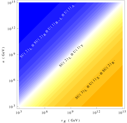
Figure 1: Phase diagram of the $\mathrm{SU(3)_{c}\otimes SU(3)_{L}\otimes SU(3)_{R}\otimes U(1)_{X}}$ electroweak theory, discussed in Sec. 5, see also Fig. 2. The Standard Model singlet VEVs $n$ and $v_{R}$ are in GeV units and their ratio is determined by Eq. (25).

5 Spontaneous symmetry breaking

In order to recover the Standard Model at low energies we need to break the $\mathrm{SU(3)_{c}\otimes SU(3)_{L}\otimes SU(3)_{R}\otimes U(1)_{X}}$ symmetry. The breaking of the gauge structure can be achieved in several ways (see Fig. 2) depending on the value of $n/v_{R}$. For $n>v_{R}\gg k_{1,2,3}$ the symmetry breaking pattern is:

$$\mathrm{SU(3)_{L}\otimes SU(3)_{R}\otimes U(1)_{X}}\xrightarrow{n}\mathrm{SU(2)_{L}\otimes SU(2)_{R}\otimes U(1)_{B-L}\otimes U(1)_{A}}\xrightarrow{v_{R}}\mathrm{SU(2)_{L}\otimes U(1)_{Y}}\hskip 2.84526pt.$$ (26)

At this stage one has $\left\langle\phi\right\rangle=\frac{1}{\sqrt{2}}\text{diag}(0,0,n)$ breaking the $T^{8}_{L,R}$ generators but preserving $T^{8}_{L}+T^{8}_{R}$, and since $\phi$ carries no $X$ charge, the resulting gauge group is $\mathrm{SU(2)_{L}\otimes SU(2)_{R}\otimes U(1)_{B-L}\otimes U(1)_{A}}$, with

$$\begin{split}&\frac{B-L}{2}=\beta(T^{8}_{L}+T^{8}_{R})+X\,,\\ &A=\beta(T^{8}_{L}+T^{8}_{R})-X\,.\end{split}$$ (27)

It is important to notice that $A$ is not involved in the electric charge definition since it reads

$$Q=T^{3}_{R}+T^{3}_{L}+\beta(T^{8}_{L}+T^{8}_{R})+X\equiv T^{3}_{R}+T^{3}_{L}+\frac{B-L}{2}\,.$$ (28)

The potential acquires the form $V=V(\phi^{\prime},\rho^{\prime},\Delta_{R}^{\prime},\Delta_{L}^{\prime},\dots)$ where

$$\begin{split}\phi^{\prime}&\sim(\mathbf{2}_{\mathrm{L}},\mathbf{2}^{*}_{\mathrm{R}},0,0)\hskip 2.84526pt,\qquad\rho^{\prime}\sim(\mathbf{2}_{\mathrm{L}},\mathbf{2}_{\mathrm{R}},0,-\frac{4q+2}{3})\hskip 2.84526pt,\\ \Delta_{L}^{\prime}&\sim(\mathbf{3}_{\mathrm{L}},\mathbf{1}_{\mathrm{R}},-1,\frac{1-4q}{3})\hskip 2.84526pt,\qquad\Delta_{R}^{\prime}\sim(\mathbf{1}_{\mathrm{L}},\mathbf{3}_{\mathrm{R}},-1,\frac{1-4q}{3})\hskip 2.84526pt,\\ \end{split}$$ (29)

are the $2\times 2$ upper left sub-matrices contained in the original $\mathrm{SU(3)_{c}\otimes SU(3)_{L}\otimes SU(3)_{R}\otimes U(1)_{X}}$ scalar multiplets in notation $\mathrm{(SU(2)_{L},SU(2)_{R},\frac{B-L}{2},A)}$, and the dots stand for the extra scalars.

Apart from the existence of the scalar multiplet $\rho$ and the extra symmetry $\mathrm{U(1)_{A}}$ the situation here resembles the popular $\mathrm{SU(3)_{c}\otimes SU(2)_{L}\otimes SU(2)_{R}\otimes U(1)_{B-L}}$ electroweak model in mohapatra:1980ia . The second step of the spontaneous symmetry breaking is carried out by $\left\langle\Delta_{R}\right\rangle=\frac{1}{\sqrt{2}}\text{diag}(v_{R},0,0)$. We note here that the generators $T_{R}^{3}$ and $A$ are broken at this stage, though the combination

$$T^{3}_{R}+\frac{B-L}{2}=Y\hskip 2.84526pt,$$ (30)

remains unbroken and hence can be identified with the Standard Model hypercharge. In this scenario, an $\mathrm{SU(2)_{L}\otimes SU(2)_{R}\otimes U(1)_{B-L}}$ structure emerges as the effective theory at lower scales. Moreover, in this case, at energy scales above $v_{R}$, we expect to observe new physics associated to a 331 model, such as virtual effects associated with exotic quarks and leptons and new gauge bosons, even if these particles are too heavy to show up directly.

Alternatively, if the VEV hierarchy is $v_{R}>n\gg k_{1,2,3}$, the symmetry breakdown follows a different route

$$\mathrm{SU(3)_{L}\otimes SU(3)_{R}\otimes U(1)_{X}}\xrightarrow{v_{R}}\mathrm{SU(3)_{L}\otimes U(1)_{X^{\prime}}\otimes SU(2)_{R^{\prime}}}\xrightarrow{n}\mathrm{SU(2)_{L}\otimes U(1)_{Y}}\hskip 2.84526pt.$$ (31)

Now $\left\langle\Delta_{R}\right\rangle=\frac{1}{\sqrt{2}}\text{diag}(v_{R},0,0)$ breaks the $\mathrm{SU(3)_{R}}$ group down to $\mathrm{SU(2)_{R^{\prime}}}$, generated by $\{T^{6}_{R},\,T^{7}_{R},\,\frac{1}{2}(\sqrt{3}T^{8}_{R}-T^{3}_{R})\}$. Simultaneously, $\mathrm{U(1)_{X}}$ is broken by $v_{R}$ but the combination $X^{\prime}=\frac{\beta+\sqrt{3}}{4}(T^{8}_{R}+\sqrt{3}T^{3}_{R})+X$ is preserved so our theory becomes an effective 331 model with an additional $\mathrm{SU(2)_{R^{\prime}}}$ symmetry at intermediate energies. In terms of the generators of the intermediate symmetries, electric charge reads

$$Q=T^{3}_{L}+T^{3}_{R}+\beta(T^{8}_{L}+T^{8}_{R})+X\equiv T^{3}_{L}+\beta T^{8}_{L}+\frac{\sqrt{3}\beta-1}{4}(\sqrt{3}T^{8}_{R}-T^{3}_{R})+X^{\prime}\,.$$ (32)

The potential in this case can be written as $V=V(\phi^{A},\phi^{B},\rho^{A},\rho^{B},\Delta_{L}^{\prime},\dots)$, where the relevant fields transform under $\mathrm{(SU(3)_{L},SU(2)_{R^{\prime}},X^{\prime})}$ as

$$\begin{split}\phi^{A}&\sim(\mathbf{3}_{\mathrm{L}},\mathbf{1}_{\mathrm{R^{\prime}}},\frac{q-1}{3})\hskip 2.84526pt,\qquad\phi^{B}\sim(\mathbf{3}_{\mathrm{L}},\mathbf{2}_{\mathrm{R^{\prime}}},\frac{1-q}{6})\hskip 2.84526pt,\\ \rho^{A}&\sim(\mathbf{3}_{\mathrm{L}},\mathbf{1}_{\mathrm{R^{\prime}}},\frac{q+2}{3})\hskip 2.84526pt,\qquad\rho^{B}\sim(\mathbf{3}_{\mathrm{L}},\mathbf{2}_{\mathrm{R^{\prime}}},\frac{5q+1}{6})\hskip 2.84526pt,\\ \Delta_{L}^{\prime}&\sim(\mathbf{6}_{\mathrm{L}},\mathbf{1}_{\mathrm{R^{\prime}}},\frac{2(q-1)}{3})\hskip 2.84526pt.\\ \end{split}$$ (33)

In a second step the triplet $\phi^{A}=\frac{1}{\sqrt{2}}(0,0,n)^{T}$ breaks the $\mathrm{SU(3)_{L}\otimes SU(2)_{R^{\prime}}\otimes U(1)_{X^{\prime}}}$ symmetry down to the Standard Model. For this VEV hierarchy, signals associated to exotic fermions are expected at intermediate energies, while new physics related to left-right symmetry, like neutrino masses, emerges at higher energies.

Finally, a third situation in which $n\sim v_{R}\gg k_{1,2,3}$ is also possible. The $\mathrm{SU(3)_{c}\otimes SU(3)_{L}\otimes SU(3)_{R}\otimes U(1)_{X}}$ gauge group in this case is broken directly to the that of the Standard Model :

$$\mathrm{SU(3)_{L}\otimes SU(3)_{R}\otimes U(1)_{X}}\xrightarrow{n,\,v_{R}}\mathrm{SU(2)_{L}\otimes U(1)_{Y}}\hskip 2.84526pt.$$ (34)

In this scenario one expects new physics associated to left-right and 331 symmetries at comparable energy scales.

Figure 2: Spontaneous symmetry breaking paths in the $\mathrm{SU(3)_{c}\otimes SU(3)_{L}\otimes SU(3)_{R}\otimes U(1)_{X}}$ electroweak theory. See also Fig. 1 and the VEV seesaw relation in Eq. (24) as well as the breaking pattern determining condition in Eq. (25).

6 Discussion and conclusion

We have proposed a fully realistic scheme based on the $\mathrm{SU(3)_{c}\otimes SU(3)_{L}\otimes SU(3)_{R}\otimes U(1)_{X}}$ gauge group. Quantum consistency requires that the number of families must match the number of colors, hence predicting the number of generations. In the simplest realization neutrino masses arise from a dynamical seesaw mechanism in which the smallness of neutrino masses is correlated with the observed V-A nature of the weak interaction. Depending on the symmetry breaking path to the Standard Model (see Figs. 1 and 2) one recovers either a $\mathrm{SU(3)_{c}\otimes SU(2)_{L}\otimes SU(2)_{R}\otimes U(1)_{B-L}}$ theory or one based on the $\mathrm{SU(3)_{c}\otimes SU(3)_{L}\otimes U(1)_{X^{\prime}}}$ gauge symmetry. This illustrates the versatility of the theory since, depending on a rather simple input parameter combination, it can mimic either of two apparently irreconcilable pictures of nature: one based upon left-right symmetry and another characterized by the $\mathrm{SU(3)_{c}\otimes SU(3)_{L}\otimes U(1)_{X^{\prime}}}$ gauge group. Either of these could be the “next” step in the quest for new physics.

Appendix A Anomaly cancellation in $\mathrm{SU(3)_{c}\otimes SU(3)_{L}\otimes SU(3)_{R}\otimes U(1)_{X}}$

In this section we outline the anomaly cancellation in the $\mathrm{SU(3)_{c}\otimes SU(3)_{L}\otimes SU(3)_{R}\otimes U(1)_{X}}$ model. The potential anomalies are $[\mathrm{SU(3)_{c}}]^{2}\otimes\mathrm{U(1)_{X}},\hskip 2.84526pt[\mathrm{SU(3)_{L}}]^{3},\hskip 2.84526pt[\mathrm{SU(3)_{R}}]^{3},\hskip 2.84526pt[\mathrm{SU(3)_{L}}]^{2}\otimes\mathrm{U(1)_{X}},\hskip 2.84526pt[\mathrm{SU(3)_{R}}]^{2}\otimes\mathrm{U(1)_{X}},\hskip 2.84526pt[\mathrm{Grav}]^{2}\otimes\mathrm{U(1)_{X}},\hskip 2.84526pt[\mathrm{U(1)_{X}}]^{3}$. First notice that the $[\mathrm{SU(3)_{c}}]^{2}\otimes\mathrm{U(1)_{X}}$ anomaly cancels straightforwardly

$$\sum_{\text{quarks}}X_{qL}-\sum_{\text{quarks}}X_{qR}=\left(-\frac{q}{3}\right)\times 3\times 3\times 2+\left(\frac{q+1}{3}\right)\times 3\times 3-\left(-\frac{q}{3}\right)\times 3\times 3\times 2-\left(\frac{q+1}{3}\right)\times 3\times 3=0\hskip 2.84526pt.$$ (35)

Since triplets and anti-triplets contribute with opposite sign to the $[\mathrm{SU(3)_{L}}]^{3}$ and $[\mathrm{SU(3)_{R}}]^{3}$ anomalies, these are only canceled if the number of triplets is equal to the number of anti-triplets, which is the case in our model. Thus from $[\mathrm{SU(3)_{R}}]^{3}$ and $[\mathrm{SU(3)_{L}}]^{3}$ we conclude that if $f$ is the number of lepton families, $n$ is the number of quark triplets and $m$ is the number of quark anti-triplets the following equation must hold:

$$3\times f+3\times 3\times n=3\times 3\times m\to f=3(m-n)\hskip 2.84526pt.$$ (36)

Next, we consider $[\mathrm{SU(3)_{L}}]^{2}\otimes\mathrm{U(1)_{X}}$ and $[\mathrm{SU(3)_{R}}]^{2}\otimes\mathrm{U(1)_{X}}$ which are canceled independently because the sum of all $X$ charges is equal to zero:

$$\begin{split}\sum_{\text{fermions}}X_{L}=\left(\frac{q-1}{3}\right)\times 3\times 3+\left(-\frac{q}{3}\right)\times 3\times 3\times 2+\left(\frac{q+1}{3}\right)\times 3\times 3=0\hskip 2.84526pt,\\ \sum_{\text{fermions}}X_{R}=\left(\frac{q-1}{3}\right)\times 3\times 3+\left(-\frac{q}{3}\right)\times 3\times 3\times 2+\left(\frac{q+1}{3}\right)\times 3\times 3=0\hskip 2.84526pt.\end{split}$$ (37)

In more general terms, this condition is the equivalent to

$$\sum_{\text{fermions}}X_{L}=\left(\frac{q-1}{3}\right)\times 3\times f+\left(-\frac{q}{3}\right)\times 3\times 3\times m+\left(\frac{q+1}{3}\right)\times 3\times 3\times n=0\hskip 2.84526pt.$$ (38)

Plugging the previous result $f=3(m-n)$ into the above relation implies that $m=2n$ and $f=3n$, independently of the value of $q$. This condition is complemented by QCD asymptotic freedom, that requires the number of quark flavors to be less than or equal to 16 leading to $3\times(m+n)=9n\leq 16$, leaving only one positive integer solution $n=1$, hence we must have $f=3$ generations.

Finally, the theory is free from gravitational anomaly $[\mathrm{Grav}]^{2}\otimes\mathrm{U(1)_{X}}$ if

$$\sum_{\text{fermions}}X_{L}=\sum_{\text{fermions}}X_{R},$$ (39)

which is trivially satisfied, while the cancellation of the $[\mathrm{U(1)_{X}}]^{3}$ anomaly follows from

$$\begin{split}\sum_{f_{L},q_{L}}X_{L}^{3}-\sum_{f_{R},q_{R}}X_{R}^{3}&=\left(\frac{q-1}{3}\right)^{3}\times 3\times 3+\left(-\frac{q}{3}\right)^{3}\times 3\times 3\times 2+\left(\frac{q+1}{3}\right)^{3}\times 3\times 3\\ &-\left(\frac{q-1}{3}\right)^{3}\times 3\times 3-\left(-\frac{q}{3}\right)^{3}\times 3\times 3\times 2-\left(\frac{q+1}{3}\right)^{3}\times 3\times 3=0\end{split}$$ (40)

Notice that L-R symmetry plays an important role in anomaly cancellation since it automatically implies that the fermion content of the model satisfy $X_{L}=X_{R}$ for every multiplet and all particles are arranged in chiral multiplets. We also remark that in our $\mathrm{SU(3)_{c}\otimes SU(3)_{L}\otimes SU(3)_{R}\otimes U(1)_{X}}$ theory the anomaly cancellation holds irrespective of the value of the $\beta$ parameter of the electric charge generator in Eq. (1).

Appendix B Acknowledgements

We thank Renato Fonseca, Martin Hirsch, P.V. Dong and D.T. Huong for useful discussions. Work supported by Spanish grants FPA2014-58183-P, Multidark CSD2009-00064, SEV-2014-0398 (MINECO) and PROMETEOII/2014/084 (Generalitat Valenciana). C.A.V-A. acknowledges support from CONACyT (Mexico), grant 274397. M. R. was supported by JAEINT-16-00831.

References

• (1) S. L. Adler, “Axial vector vertex in spinor electrodynamics,” Phys.Rev. 177 (1969) 2426–2438.
• (2) J. Bell and R. Jackiw, “A PCAC puzzle: $\pi^{0}\to\gamma\gamma$ in the sigma model,” Nuovo Cim. A60 (1969) 47–61.
• (3) J. C. Pati and A. Salam, “Lepton number as the fourth color,” Phys. Rev. D10 (1974) 275–289.
• (4) M. Gell-Mann, P. Ramond, and R. Slansky, “Complex Spinors and Unified Theories,” Conf. Proc. C790927 (1979) 315–321, arXiv:1306.4669 [hep-th].
• (5) T. Yanagida, “Horizontal symmetry and masses of neutrinos,” Conf. Proc. C7902131 (1979) 95–99.
• (6) R. N. Mohapatra and G. Senjanovic, “Neutrino mass and spontaneous parity nonconservation,” Phys. Rev. Lett. 44 (1980) 91.
• (7) J. Schechter and J. Valle, “Neutrino Masses in SU(2) x U(1) Theories,” Phys.Rev. D22 (1980) 2227.
• (8) G. Lazarides, Q. Shafi, and C. Wetterich, “Proton lifetime and fermion masses in an SO(10) model,” Nucl. Phys. B181 (1981) 287.
• (9) M. Singer, J. Valle, and J. Schechter, “Canonical Neutral Current Predictions From the Weak Electromagnetic Gauge Group SU(3) X $u$(1),” Phys.Rev. D22 (1980) 738.
• (10) J. W. F. Valle and M. Singer, “Lepton number violation with quasi Dirac neutrinos,” Phys. Rev. D28 (1983) 540.
• (11) S. M. Boucenna, S. Morisi, and J. W. F. Valle, “Radiative neutrino mass in 3-3-1 scheme,” Phys. Rev. D90 no. 1, (2014) 013005, arXiv:1405.2332 [hep-ph].
• (12) S. M. Boucenna, R. M. Fonseca, F. Gonzalez-Canales, and J. W. F. Valle, “Small neutrino masses and gauge coupling unification,” Phys. Rev. D91 no. 3, (2015) 031702, arXiv:1411.0566 [hep-ph].
• (13) J. C. Montero, C. A. De S. Pires, and V. Pleitez, “Neutrino masses through the seesaw mechanism in 3-3-1 models,” Phys. Rev. D65 (2002) 095001, arXiv:hep-ph/0112246 [hep-ph].
• (14) M. E. Catano, R. Martinez, and F. Ochoa, “Neutrino masses in a 331 model with right-handed neutrinos without doubly charged Higgs bosons via inverse and double seesaw mechanisms,” Phys. Rev. D86 (2012) 073015, arXiv:1206.1966 [hep-ph].
• (15) A. Addazi, J. W. F. Valle, and C. A. Vaquera-Araujo, “String completion of an $\mathrm{SU(3)_{c}\otimes SU(3)_{L}\otimes U(1)_{X}}$ electroweak model,” Phys. Lett. B759 (2016) 471–478, arXiv:1604.02117 [hep-ph].
• (16) J. W. F. Valle and C. A. Vaquera-Araujo, “Dynamical seesaw mechanism for Dirac neutrinos,” Phys. Lett. B755 (2016) 363–366, arXiv:1601.05237 [hep-ph].
• (17) M. Reig, J. W. F. Valle, and C. A. Vaquera-Araujo, “Realistic $\mathrm{SU(3)_{c}\otimes SU(3)_{L}\otimes U(1)_{X}}$ model with a type II Dirac neutrino seesaw mechanism,” Phys. Rev. D94 no. 3, (2016) 033012, arXiv:1606.08499 [hep-ph].
• (18) A. G. Dias, C. A. de S. Pires, and P. S. Rodrigues da Silva, “The Left-Right SU(3)(L)xSU(3)(R)xU(1)(X) Model with Light, keV and Heavy Neutrinos,” Phys. Rev. D82 (2010) 035013, arXiv:1003.3260 [hep-ph].
• (19) C. P. Ferreira, M. M. Guzzo, and P. C. de Holanda, “Cosmological bounds of sterile neutrinos in a $SU(3)_{C}\otimes SU(3)_{L}\otimes SU(3)_{R}\otimes U(1)_{N}$ model as dark matter candidates,” Braz. J. Phys. 46 no. 4, (2016) 453–461, arXiv:1509.02977 [hep-ph].
• (20) D. T. Huong and P. V. Dong, “Left-right asymmetry and 750 GeV diphoton excess,” Phys. Rev. D93 no. 9, (2016) 095019, arXiv:1603.05146 [hep-ph].
• (21) P. V. Dong and D. T. Huong, “Left-right model for dark matter,” arXiv:1610.02642 [hep-ph].
• (22) A. J. Buras, F. De Fazio, and J. Girrbach-Noe, “Z-Z’ mixing and Z-mediated FCNCs in SU(3)C x SU(3)L x U(1)X models,” JHEP 1408 (2014) 039, arXiv:1405.3850 [hep-ph].
• (23) R. M. Fonseca and M. Hirsch, “A flipped 331 model,” JHEP 08 (2016) 003, arXiv:1606.01109 [hep-ph].
• (24) R. M. Fonseca and M. Hirsch, “Lepton number violation in 331 models,” arXiv:1607.06328 [hep-ph].
• (25) P. Langacker and G. Steigman, “Requiem for an FCHAMP? Fractionally CHArged, Massive Particle,” Phys. Rev. D84 (2011) 065040, arXiv:1107.3131 [hep-ph].