Caratheodory-Tchakaloff Subsampling

Abstract

We present a brief survey on the compression of discrete measures by Caratheodory-Tchakaloff Subsampling, its implementation by Linear or Quadratic Programming and the application to multivariate polynomial Least Squares. We also give an algorithm that computes the corresponding Caratheodory-Tchakaloff (CATCH) points and weights for polynomial spaces on compact sets and manifolds in 2D and 3D.

2010 AMS subject classification: 41A10, 65D32, 93E24. Keywords: multivariate discrete measures, compression, subsampling, Tchakaloff theorem, Caratheodory theorem, Linear Programming, Quadratic Programming, polynomial Least Squares, polynomial meshes.

1 Subsampling for discrete measures

Tchakaloff theorem, a cornerstone of quadrature theory, substantially asserts that for every compactly supported measure there exists a positive algebraic quadrature formula with cardinality not exceeding the dimension of the exactness polynomial space (restricted to the measure support). Originally proved by V. Tchakaloff in 1957 for absolutely continuous measures [29], it has then be extended to any measure with finite polynomial moments, cf. e.g. [10], and to arbitrary finite dimensional spaces of integrable functions [1].

We begin by stating a discrete version of Tchakaloff theorem, in its full generality, whose proof is based on Caratheodory theorem about finite dimensional conic combinations.

Theorem 1

Let $\mu$ be a multivariate discrete measure supported at a finite set $X=\{x_{i}\}\subset\mathbb{R}^{d}$, with correspondent positive weights (masses) $\boldsymbol{\lambda}=\{\lambda_{i}\}$, $i=1,\dots,M$, and let $S=\mbox{span}(\phi_{1},\dots,\phi_{L})$ a finite dimensional space of $d$-variate functions defined on $K\supseteq X$, with $N=\mbox{dim}(S|_{X})\leq L$.

Then, there exist a quadrature formula with nodes $T=\{t_{j}\}\subseteq X$ and positive weights $\boldsymbol{w}=\{w_{j}\}$, $1\leq j\leq m\leq N$, such that

$$\int_{X}{f(x)\,d\mu}=\sum_{i=1}^{M}{\lambda_{i}\,f(x_{i})}=\sum_{j=1}^{m}{w_{j}\,f(t_{j})}\;,\;\;\forall f\in S|_{X}\;.$$ (1)

Proof. Let $\{\psi_{1},\dots,\psi_{N}\}$ be a basis of $S|_{X}$, and $V=(v_{ij})=(\psi_{j}(x_{i}))$ the Vandermonde-like matrix of the basis computed at the support points. If $M>N$ (otherwise there is nothing to prove), existence of a positive quadrature formula for $\mu$ with cardinality not exceeding $N$ can be immediately translated into existence of a nonnegative solution with at most $N$ nonvanishing components to the underdetermined linear system

$$V^{t}\boldsymbol{u}=\boldsymbol{b}\;,\;\;\boldsymbol{u}\geq\boldsymbol{0}\;,$$ (2)

where

$$\boldsymbol{b}=V^{t}\boldsymbol{\lambda}=\left\{\int_{X}{\psi_{j}(x)\,d\mu}\right\}\;,\;\;1\leq j\leq N\;,$$ (3)

is the vector of $\mu$-moments of the basis $\{\psi_{j}\}$.

Existence then holds by the well-known Caratheodory theorem applied to the columns of $V^{t}$, which asserts that a conic (i.e., with positive coefficients) combination of any numer of vectors in $\mathbb{R}^{N}$ can be rewritten as a conic combination of at most $N$ (linearly independent) of them; cf. [8] and, e.g., [9, §3.4.4].$\;\;\;\;\;\square$

Since such a discrete version of Tchakaloff theorem is a direct consequence of Caratheodory theorem, we may term such an approach Caratheodory-Tchakaloff subsampling, and the corresponding nodes (with associated weights) a set of Caratheodory-Tchakaloff (CATCH) points.

The idea of reduction/compression of a finite measure by Tchakaloff or directly Caratheodory theorem recently arose in different contexts, for example in a probabilistic setting [16], as well as in univariate [13] and multivariate [2, 20, 25, 28] numerical quadrature, with applications to multivariate polynomial inequalities and least squares approximation [20, 28, 31]. In many situations CATCH subsampling can produce a high Compression Ratio, namely when $N\ll M$ like for example in polynomial least squares approximation [28] or in QMC (Quasi-Monte Carlo) integration [2] or in particle methods [16],

$$C_{ratio}=\frac{M}{m}\geq\frac{M}{N}\gg 1\;,$$ (4)

so that the efficient computation of CATCH points and weights becomes a relevant task.

Now, while the proof of the general Tchakaloff theorem is not, that of the discrete version can be made constructive, since Caratheodory theorem itself has a constructive proof (cf., e.g., [9, §3.4.4]). On the other hand, such a proof does not give directly an efficient implementation. Nevertheless, there are at least two reasonably efficient approaches to solve the problem.

The first, adopted for example in [13] (univariate) and [28] (multivariate) in the framework of polynomial spaces, rests on Quadratic Programming, namely on the classical Lawson-Hanson active set method for NonNegative Least Squares (NLLS). Indeed, we may think to solve the quadratic minimum problem

$$\mbox{NNLS}:\;\;\;\left\{\begin{array}[]{ll}\min{\|V^{t}\boldsymbol{u}-\boldsymbol{b}\|_{2}}\\ \boldsymbol{u}\geq\boldsymbol{0}\end{array}\right.$$ (5)

which exists by Theorem 1 and can be computed by standard NNLS solvers based on the Lawson-Hanson method [15], which seeks a sparse solution. Then, the nonvanishing components of such a solution give the weights $\boldsymbol{w}=\{w_{j}\}$ as well as the indexes of the nodes $T=\{t_{j}\}$ within $X$. A variant of the Lawson-Hanson method is implemented in the Matlab native function lsqnonneg [17], while a recent optimized Matlab implementation can be found in [26].

The second approach is based instead on Linear Programming via the classical simplex method. Namely, we may think to solve the linear minimum problem

$$\mbox{LP}:\;\;\;\left\{\begin{array}[]{ll}\min{\boldsymbol{c}^{t}\boldsymbol{u}}\\ V^{t}\boldsymbol{u}=\boldsymbol{b}\;,\;\;\boldsymbol{u}\geq\boldsymbol{0}\end{array}\right.$$ (6)

where the constraints identify a polytope (the feasible region) in $\mathbb{R}^{d}$ and the vector $\boldsymbol{c}$ is chosen to be linearly independent from the rows of $V^{t}$ (i.e., it is not the restriction to $X$ of a function in $S$), so that the objective functional is not constant on the polytope. To this aim, if $X\subset K$ is determining on a supspace $T\supset S$ on $K$, i.e. a function in $T$ vanishing on $X$ vanishes everywhere on $K$, then it is sufficient to take $\boldsymbol{c}=\{g(x_{i})\}$, $1\leq i\leq M$, where the function $g|_{K}$ belongs to $T|_{K}\setminus S|_{K}$. For example, working with polynomials it is sufficient to take a polynomial of higher degree on $K$ with respect to those in $S|_{K}$.

Observe that in our setting the feasible region is nonempty, since $\boldsymbol{b}=V^{t}\boldsymbol{\lambda}$, and we are interested in any basic feasible solution, i.e., in any vertex of the polytope, that has at least $M-N$ vanishing components. As it is well-known, the solution of the Linear Programming problem is a vertex of the polytope that can be computed by the simplex method (cf., e.g., [9]). Again, the nonvanishing components of such a vertex give the weights $\boldsymbol{w}=\{w_{j}\}$ as well as the indexes of the nodes $T=\{t_{j}\}$ within $X$.

This approach was adopted for example in [25] as a basic step to compute, when it exists, a multivariate algebraic Gaussian quadrature formula (suitable choices of $\boldsymbol{c}$ are also discussed there; see Example 1 below). In a Matlab-like environment, the simplex method is implemented by the glpk Octave native function [19] (from the GNU Linear Programming Kit).

Even though both, the active set method for (5) and the simplex method for (6), have theoretically an exponential complexity (worst case analysis), as it is well-known their practical behavior is quite satisfactory, since the average complexity turns out to be polynomial in the dimension of the problems (observe that in the present setting we deal with dense matrices); cf., e.g., [12, Ch. 9]. It is worth quoting here the extensive theoretical and computational results recently presented in the Ph.D. dissertation [30], where Caratheodory reduction of a discrete measure is implemented by Linear Programming, claiming an experimental average cost of $\mathcal{O}(N^{3.7})$.

A different combinatorial algorithm (Recursive Halving Forest), based on the SVD, is also there proposed to compute a basic feasible solution and compared with the best Linear Programming solvers, claiming an experimental average cost of $\mathcal{O}(N^{2.6})$. The methods are essentially applied to the reduction of Cartesian tensor cubature measures.

In our implementation of CATCH subsampling [21], we have chosen to work with the Octave native Linear Programming solver glpk and the Matlab native Quadratic Programming solver lsqnonneg, that are suitable for moderate size problems, like those typically arising with polynomial spaces ($S=S_{\nu}=\mathbb{P}_{\nu}^{d}$) in dimension $d=2,3$ and small/moderate degree of exactness $\nu$. On large size problems, like those typically arising in higher dimension and/or high degree of exactness, the solvers discussed in [30] could become necessary.

Now, since we may expect that the underdetermined system (2) is not satisfied exactly by the computed solution, due to finite precision arithmetic and by the effect of an error tolerance in the iterative algorithms, namely that there is a nonzero moment residual

$$\|V^{t}\boldsymbol{u}-\boldsymbol{b}\|_{2}=\varepsilon>0\;,$$ (7)

it is then worth studying the effect of such a residual on the accuracy of the quadrature formula. We can state and prove an estimate still in the general discrete setting of Theorem 1.

Proposition 1

Let the assumptions of Theorem 1 be satisfied, let $\boldsymbol{u}$ be a nonnegative vector such that (7) holds, where $V$ is the Vandermonde-like matrix at $X$ corresponding to a $\mu$-orthonormal basis $\{\psi_{k}\}$ of $S|_{X}$, and let $(T,\boldsymbol{w})$ be the quadrature formula corresponding to the nonvanishing components of $\boldsymbol{u}$. Moreover, let $1\in S$ (i.e., $S$ contains the constant functions).

Then, for every function $f$ defined on $X$, the following error estimate holds

$$\left|\int_{X}{f(x)\,d\mu}-\sum_{j=1}^{m}{w_{j}\,f(t_{j})}\right|\leq C_{\varepsilon}E_{S}(f;X)+\varepsilon\|f\|_{\ell^{2}_{\boldsymbol{\lambda}}(X)}\;,$$ (8)

where

$$E_{S}(f;X)=\min_{\phi\in S}{\|f-\phi\|_{\ell^{\infty}(X)}}\;,\;\;C_{\varepsilon}=2\left(\mu(X)+\varepsilon\,\sqrt{\mu(X)}\right)\;.$$ (9)

Proof. First, observe that

$$\int_{X}{\phi(x)\,d\mu}=\langle\boldsymbol{\gamma},\boldsymbol{b}\rangle\;,\;\;\forall\phi\in S\;,$$ (10)

$\boldsymbol{\gamma}=\{\gamma_{k}\}$, $\boldsymbol{b}=\{b_{k}\}=V^{t}\boldsymbol{\lambda}$, where $\langle\cdot,\cdot\rangle$ denotes the Euclidean scalar product in $\mathbb{R}^{N}$ and

$$\gamma_{k}=\int_{X}{\phi(x)\psi_{k}(x)\,d\mu}\;,\;\;b_{k}=\int_{X}{\psi_{k}(x)\,d\mu}\;,\;\;1\leq k\leq N\;,$$

are the coefficients of $\phi$ in the $\mu$-orthonormal basis $\{\psi_{k}\}$ and the $\mu$-moments of $\{\psi_{k}\}$, respectively.

Take $\phi\in S$. By a classical chain of estimates in quadrature theory, we can write

$$\left|\int_{X}{f(x)\,d\mu}-\sum_{j=1}^{m}{w_{j}\,f(t_{j})}\right|\leq\int_{X}{|f(x)-\phi(x)|\,d\mu}$$

$$+\left|\int_{X}{\phi(x)\,d\mu}-\sum_{j=1}^{m}{w_{j}\,\phi(t_{j})}\right|+\sum_{j=1}^{m}{w_{j}\,|\phi(t_{j})-f(t_{j})|}$$

$$\leq\left(\mu(X)+\sum_{j=1}^{m}{w_{j}}\right)\|f-\phi\|_{\ell^{\infty}(X)}+\left|\int_{X}{\phi(x)\,d\mu}-\sum_{j=1}^{m}{w_{j}\,\phi(t_{j})}\right|\;.$$ (11)

Now,

$$\sum_{j=1}^{m}{w_{j}\,\phi(t_{j})}=\sum_{k=1}^{N}{\gamma_{k}\,\sum_{j=1}^{m}{w_{j}\,\psi_{k}(t_{j})}}=\langle\boldsymbol{\gamma},V^{t}\boldsymbol{u}\rangle\;,$$

and thus by the Cauchy-Schwarz inequality

$$\left|\int_{X}{\phi(x)\,d\mu}-\sum_{j=1}^{m}{w_{j}\,\phi(t_{j})}\right|=|\langle\boldsymbol{\gamma},b-V^{t}\boldsymbol{u}\rangle|\leq\|\boldsymbol{\gamma}\|_{2}\,\|b-V^{t}\boldsymbol{u}\|_{2}=\|\phi\|_{\ell^{2}_{\boldsymbol{\lambda}}(X)}\,\varepsilon\;.$$ (12)

Moreover

$$\|\phi\|_{\ell^{2}_{\boldsymbol{\lambda}}(X)}\leq\|\phi-f\|_{\ell^{2}_{\boldsymbol{\lambda}}(X)}+\|f\|_{\ell^{2}_{\boldsymbol{\lambda}}(X)}$$

$$\leq\sqrt{\mu(X)}\,\|\phi-f\|_{\ell^{\infty}(X)}+\|f\|_{\ell^{2}_{\boldsymbol{\lambda}}(X)}\;.$$ (13)

On the other hand

$$\sum_{j=1}^{m}{w_{j}}\leq\left|\sum_{j=1}^{m}{w_{j}}-\int_{X}{1\,d\mu}\right|+\int_{X}{1\,d\mu}=\left|\sum_{j=1}^{m}{w_{j}}-\int_{X}{1\,d\mu}\right|+\mu(X)$$

$$\leq\varepsilon\,\|1\|_{\ell^{2}_{\boldsymbol{\lambda}}(X)}+\mu(X)=\varepsilon\,\sqrt{\mu(X)}+\mu(X)\;,$$ (14)

where we have applied (12) with $\phi=1$.

Putting estimates (12)-(14) into (11 we obtain

$$\left|\int_{X}{f(x)\,d\mu}-\sum_{j=1}^{m}{w_{j}\,f(t_{j})}\right|\leq\left(2\mu(X)+\varepsilon\,\sqrt{\mu(X)}\right)\|f-\phi\|_{\ell^{\infty}(X)}$$

$$+\varepsilon\left(\sqrt{\mu(X)}\,\|\phi-f\|_{\ell^{\infty}(X)}+\|f\|_{\ell^{2}_{\boldsymbol{\lambda}}(X)}\right)\;,\;\;\forall\phi\in S\;,$$

and taking the minimum over $\phi\in S$ we finally get (8). $\;\;\;\;\;\square$

It is worth observing that the assumption $1\in S$ is quite natural, being satisfied for example in the usual polynomial and trigonometric spaces. From this point of view, we can also stress that sparsity cannot be ensured by the standard Compressive Sensing approach to underdetermined systems, such as the Basis Pursuit algorithm that minimizes $\|u\|_{1}$ (cf., e.g., [11]), since if $1\in S$ then $\|u\|_{1}=\mu(X)$ is constant.

Moreover, we notice that if $K\supset X$ is a compact set, then

$$E_{S}(f;X)\leq E_{S}(f;K)\;,\;\;\forall f\in C(K)\;.$$ (15)

If $S$ is a polynomial space (as in the sequel) and $K$ is a “Jackson compact”, $E_{S}(f;K)$ can be estimated by the regularity of $f$ via multivariate Jackson-like theorems; cf. [24].

To conclude this Section, we sketch the pseudo-code of an algorithm that implements CATCH subsampling, via the preliminary computation of an orthonormal basis of $S|_{X}$.

Algorithm 1

(computation of CATCH points and weights):

• input: the discrete measure $(X,\boldsymbol{\lambda})$, the generators $(\phi_{k})=(\phi_{1},\dots,\phi_{L})$ of $S$, possibly the dimension $N$ of $S|_{X}$

• compute the Vandermode-like matrix $U=(u_{ik})=(\phi_{k}(x_{i}))$

• if $N$ is unknown, compute $N=rank(U)$ by a rank-revealing algorithm

• compute the QR factorization with column pivoting $\sqrt{\Lambda}\,U(:,\boldsymbol{\pi})=QR$, where $\Lambda=diag(\lambda_{i})$ and $\boldsymbol{\pi}$ is a permutation vector (we observe that $rank(Q)=rank(\sqrt{\Lambda}\,U)=rank(U)=N$)

• select the orthogonal matrix $V=Q(:,1:N)$; the first $N$ columns of $Q$ correspond to an orthonormal basis of $S|_{X}$ with respect to the measure $(X,\boldsymbol{\lambda})$, $(\psi_{j})=(\phi_{\pi_{j}})R_{N}^{-1}$, $1\leq j\leq N$, where $R_{N}=R(1:N,1:N)$

• compute a sparse solution to $V^{t}\boldsymbol{u}=\boldsymbol{b}=V^{t}\boldsymbol{\lambda}$, $\boldsymbol{u}\geq\boldsymbol{0}$, by the Lawson-Hanson method for the NNLS problem (5) or by the simplex method for the LP problem (6)

• compute the residual $\varepsilon=\|V^{t}\boldsymbol{u}-\boldsymbol{b}\|_{2}$

• $ind=\{i:u_{i}\neq 0\}$, $\boldsymbol{w}=\boldsymbol{u}(ind)$, $T=X(ind)$

• output: the CATCH compressed measure $(T,\boldsymbol{w})$ and the residual $\varepsilon$ (that appears in the relevant estimates (8)-(9))

 

We observe that there are two key tools of numerical linear algebra in this algorithm, that allow to work in the right space, in view of the fact that $rank(U)=\mbox{dim}(S|_{X})$. The first is the computation of such a rank, that gives of course a numerical rank, due to finite precision arithmetic. Here we can resort, for example, to the SVD decomposition of $U$ in its less costly version that produces only the singular values (with a threshold on such values), which is just that used by the rank Matlab/Octave native function. The second is the computation of a basis of $S|_{X}$, namely an orthonormal basis, by the pivoting process which is aimed at selecting linearly independent generators.

2 Caratheodory-Tchakaloff Least Squares

The case where $(X,\boldsymbol{\lambda})$ is itself a quadrature/cubature formula for some measure on $K\supset X$, that is the compression (or reduction) of such formulas, has been till now the main application of Caratheodory-Tchakaloff subsampling, in the classical framework of algebraic formulas as well as in the probabilistic/QMC framework; cf. [13, 25, 28] and [2, 16, 30]. In this survey, we concentrate on another relevant application, that is the compression of multivariate polynomial least squares.

Let us consider the total-degree polynomial framework, that is

$$S=S_{\nu}=\mathbb{P}_{\nu}^{d}(K)\;,$$ (16)

the space of $d$-variate real polynomials with total-degree not exceeding $\nu$, restricted to $K\subset\mathbb{R}^{d}$, a compact set or a compact (subset of a) manifold. Let us define for notational convenience

$$E_{n}(f)=E_{\mathbb{P}_{n}^{d}(K)}(f;K)=\min_{p\in\mathbb{P}_{n}^{d}(K)}{\|f-p\|_{L^{\infty}(K)}}\;,$$ (17)

where $f\in C(K)$.

Discrete LS approximation by total-degree polynomials of degree at most $n$ on $X\subset K$ is ultimately an orthogonal projection of a function $f$ on $\mathbb{P}_{n}^{d}(X)$, with respect to the scalar product of $\ell^{2}(X)$, namely

$$\|f-\mathcal{L}_{n}f\|_{\ell^{2}(X)}=\min_{p\in\mathbb{P}_{n}^{d}(K)}{\|f-p\|_{\ell^{2}(X)}}=\min_{p\in\mathbb{P}^{d}_{n}(X)}{\|f-p\|_{\ell^{2}(X)}}\;.$$ (18)

Recall that for every function $g$ defined on $X$

$$\|g\|^{2}_{\ell^{2}(X)}=\sum_{i=1}^{M}{g^{2}(x_{i})}=\int_{X}{g^{2}(x)\,d\mu}\;,$$ (19)

where $\mu$ is the discrete measure supported at $X$ with unit masses $\boldsymbol{\lambda}=(1,\dots,1)$.

Taking $p^{\ast}\in\mathbb{P}^{d}_{n}(X)$ such that $\|f-p^{\ast}\|_{\ell^{\infty}(X)}$ is minimum (the polynomial of best uniform approximation of $f$ in $\mathbb{P}^{d}_{n}(X)$), we get immediately the classical LS error estimate

$$\|f-\mathcal{L}_{n}f\|_{\ell^{2}(X)}\leq\|f-p^{\ast}\|_{\ell^{2}(X)}\leq\sqrt{M}\,\|f-p^{\ast}\|_{\ell^{\infty}(X)}\leq\sqrt{M}\,E_{n}(f)\;,$$ (20)

where $M=\mu(X)=\mbox{card}(X)$. In terms of the Root Mean Square Error (RMSE), an indicator widely used in the applications, we have

$$\mbox{RMSE}_{X}(\mathcal{L}_{n}f)=\frac{1}{\sqrt{M}}\,\|f-\mathcal{L}_{n}f\|_{\ell^{2}(X)}\leq E_{n}(f)\;.$$ (21)

Now, if $M>N_{2n}=\mbox{dim}(\mathbb{P}_{2n}^{d}(X))$ (we stress that here polynomials of degree $2n$ are involved), by Theorem 1 there exist $m\leq N_{2n}$ Caratheodory-Tchakaloff (CATCH) points $T_{2n}=\{t_{j}\}$ and weights $\boldsymbol{w}=\{w_{j}\}$, $1\leq j\leq m$, such that the following basic $\ell^{2}$ identity holds

$$\|p\|^{2}_{\ell^{2}(X)}=\sum_{i=1}^{M}{p^{2}(x_{i})}=\sum_{j=1}^{m}{w_{j}\,p^{2}(t_{j})}=\|p\|^{2}_{\ell^{2}_{\boldsymbol{w}}(T_{2n})}\;,\;\;\forall p\in\mathbb{P}^{d}_{n}(X)\;.$$ (22)

Notice that the CATCH points $T_{2n}\subset X$ are $\mathbb{P}^{d}_{n}(X)$-determining, i.e., a polynomial of degree at most $n$ vanishing there vanishes everywhere on $X$, or in other terms $\mbox{dim}(\mathbb{P}^{d}_{n}(T_{2n}))=\mbox{dim}(\mathbb{P}^{d}_{n}(X))$, or equivalently any Vandermonde-like matrix with a basis of $\mathbb{P}^{d}_{n}(X)$ at $T_{2n}$ has full rank. This also entails that, if $X$ is $\mathbb{P}^{d}_{n}(K)$-determining, then such is $T_{2n}$.

Consider the $\ell^{2}_{\boldsymbol{w}}(T_{2n})$ LS polynomial $\mathcal{L}_{n}^{c}f$, namely

$$\|f-\mathcal{L}_{n}^{c}f\|_{\ell^{2}_{\boldsymbol{w}}(T_{2n})}=\min_{p\in\mathbb{P}_{n}^{d}(K)}{\|f-p\|_{\ell^{2}_{\boldsymbol{w}}(T_{2n})}}=\min_{p\in\mathbb{P}^{d}_{n}(X)}{\|f-p\|_{\ell^{2}_{\boldsymbol{w}}(T_{2n})}}\;.$$ (23)

Notice that $\mathcal{L}_{n}^{c}$ is a weighted least squares operator; reasoning as in (21) and observing that $\sum_{j=1}^{m}{w_{j}}=M$ since $1\in\mathbb{P}^{d}_{n}$, we get immediately

$$\|f-\mathcal{L}_{n}^{c}f\|_{\ell^{2}_{\boldsymbol{w}}(T_{2n})}\leq\sqrt{M}\,E_{n}(f)\;.$$ (24)

On the other hand, we can also write the following estimates

$$\|f-\mathcal{L}_{n}^{c}f\|_{\ell^{2}(X)}\leq\|f-p^{\ast}\|_{\ell^{2}(X)}+\|\mathcal{L}_{n}^{c}(p^{\ast}-f)\|_{\ell^{2}(X)}$$

and

$$\|\mathcal{L}_{n}^{c}(p^{\ast}-f)\|_{\ell^{2}(X)}=\|\mathcal{L}_{n}^{c}(p^{\ast}-f)\|_{\ell^{2}_{\boldsymbol{w}}(T_{2n})}\leq\|p^{\ast}-f\|_{\ell^{2}_{\boldsymbol{w}}(T_{2n})}\;,$$

where we have used the basic $\ell^{2}$ identity (22), the fact that $\mathcal{L}_{n}^{c}p^{\ast}=p^{\ast}$ and that $\mathcal{L}_{n}^{c}f$ is an orthogonal projection. By the two estimates above we get eventually

$$\|f-\mathcal{L}_{n}^{c}f\|_{\ell^{2}(X)}\leq\sqrt{M}\,\left(\|f-p^{\ast}\|_{\ell^{\infty}(X)}+\|f-p^{\ast}\|_{\ell^{\infty}(T_{2n})}\right)\leq 2\sqrt{M}\,E_{n}(f)\;,$$ (25)

or, in RMSE terms,

$$\mbox{RMSE}_{X}(\mathcal{L}_{n}^{c}f)\leq 2E_{n}(f)\;,$$ (26)

which shows the most relevant feature of the “compressed” least squares operator $\mathcal{L}_{n}^{c}$ at the CATCH points (CATCHLS), namely that

• the LS and compressed CATCHLS RMSE estimates (21) and (26) have substantially the same size.

This fact, in particular the appearance of the factor $2$ in the estimate for the compressed operator, is reminiscent of hyperinterpolation theory [27]. Indeed, what we are constructing here is a sort of hyperinterpolation in a fully discrete setting. Roughly summarizing, hyperinterpolation ultimately approximates a (weighted) $L^{2}$ projection on $\mathbb{P}_{n}^{d}$ by a discrete weighted $\ell^{2}$ projection, via a quadrature formula of exactness degree $2n$. Similarly, here we are approximating a $\ell^{2}$ projection on $\mathbb{P}_{n}^{d}$ by a weighted $\ell^{2}$ projection with a smaller support, again via a quadrature formula of exactness degree $2n$.

The estimates above are valid by the theoretical exactness of the quadrature formula. In order to take into account a nonzero moment residual as in (7), we state and prove the following

Proposition 2

Let $\mu$ be the discrete measure supported at $X$ with unit masses $\boldsymbol{\lambda}=(1,\dots,1)$, let $\boldsymbol{u}$ be a nonnegative vector such that (7) holds, where $V$ is the orthogonal Vandermonde-like matrix at $X$ corresponding to a $\mu$-orthonormal basis $\{\psi_{k}\}$ of $\mathbb{P}^{d}_{2n}(X)$, and let $(T_{2n},\boldsymbol{w})$ be the quadrature formula corresponding to the nonvanishing components of $\boldsymbol{u}$. Then the following polynomial inequalities hold for every $p\in\mathbb{P}^{d}_{n}(X)$

$$\|p\|_{\ell^{2}(X)}\leq\alpha_{M}(\varepsilon)\,\|p\|_{\ell^{2}_{\boldsymbol{w}}(T_{2n})}\leq\sqrt{M}\,\beta_{M}(\varepsilon)\,\|p\|_{\ell^{\infty}(T_{2n})}\;,$$ (27)

where

$$\alpha_{M}(\varepsilon)=\left(1-\varepsilon\sqrt{M}\right)^{-1/2}\;,\;\;\beta_{M}(\varepsilon)=\alpha_{M}(\varepsilon)\,\left(1+\varepsilon/\sqrt{M}\right)^{1/2}\;,$$ (28)

provided that $\varepsilon\sqrt{M}<1$.

Corollary 1

Let the assumptions of Proposition 2 be satisfied. Then the following error estimate holds for every $f\in C(K)$

$$\|f-\mathcal{L}_{n}^{c}f\|_{\ell^{2}(X)}\leq\left(1+\beta_{M}(\varepsilon)\right)\,\sqrt{M}\,E_{n}(f)\;.$$ (29)

Proof of Proposition 2 and Corollary 1. First, observe that

$$\|p\|^{2}_{\ell^{2}(X)}=\int_{X}{p^{2}(x)\,d\mu}=\sum_{j=1}^{m}{w_{j}\,p^{2}(t_{j})}+\varepsilon_{2n}$$

$$\leq\sum_{j=1}^{m}{w_{j}\,p^{2}(t_{j})}+|\varepsilon_{2n}|=\|p\|^{2}_{\ell^{2}_{\boldsymbol{w}}(T_{2n})}+|\varepsilon_{2n}|\;,$$

where by Proposition 1

$$|\varepsilon_{2n}|\leq\varepsilon\|p^{2}\|_{\ell^{2}(X)}\;.$$

Now, using the fact that we are in a fully discrete setting, we get

$$\|p^{2}\|_{\ell^{2}(X)}\leq\sqrt{M}\,\|p^{2}\|_{\ell^{\infty}(X)}=\sqrt{M}\,\|p\|^{2}_{\ell^{\infty}(X)}\leq\sqrt{M}\,\|p\|^{2}_{\ell^{2}(X)}\;,$$

and finally putting together the three estimates above

$$\|p\|^{2}_{\ell^{2}(X)}\leq\|p\|^{2}_{\ell^{2}_{\boldsymbol{w}}(T_{2n})}+\varepsilon\sqrt{M}\,\|p\|^{2}_{\ell^{2}(X)}\;,$$

that is the first inequality in (27), provided that $\varepsilon\sqrt{M}<1$. To get the second inequality in (27), we simply observe that for every function $g$ defined on $X$

$$\|g\|^{2}_{\ell^{2}_{\boldsymbol{w}}(T_{2n})}\leq\left(\sum_{j=1}^{m}{w_{j}}\right)\,\|g\|^{2}_{\ell^{\infty}(T_{2n})}\leq M\,\left(1+\varepsilon/\sqrt{M}\right)\,\|g\|^{2}_{\ell^{\infty}(T_{2n})}$$ (30)

in view of (14) (here $\mu(X)=M$). We notice incidentally that the estimates in [28, §4] must be corrected, since the factor $(1+\varepsilon/\sqrt{M})^{1/2}$ is missing there.

Concerning Corollary 1, take $p^{\ast}\in\mathbb{P}^{d}_{n}(X)$ such that $\|f-p^{\ast}\|_{\ell^{\infty}(X)}$ is minimum (the polynomial of best uniform approximation of $f$ in $\mathbb{P}^{d}_{n}(X)$). Then we can write, in view of Proposition 1 and the fact that $\mathcal{L}_{n}^{c}$ is an orthogonal projection operator in $\ell^{2}_{\boldsymbol{w}}(T_{2n})$,

$$\|f-\mathcal{L}_{n}^{c}f\|_{\ell^{2}(X)}\leq\|f-p^{\ast}\|_{\ell^{2}(X)}+\|\mathcal{L}_{n}^{c}(p^{\ast}-f)\|_{\ell^{2}(X)}$$

$$\leq\sqrt{M}\,\|f-p^{\ast}\|_{\ell^{\infty}(X)}+\alpha_{M}(\varepsilon)\,\|\mathcal{L}_{n}^{c}(p^{\ast}-f)\|_{\ell^{2}_{\boldsymbol{w}}(T_{2n})}$$

$$\leq\sqrt{M}\,\|f-p^{\ast}\|_{\ell^{\infty}(X)}+\alpha_{M}(\varepsilon)\,\|p^{\ast}-f\|_{\ell^{2}_{\boldsymbol{w}}(T_{2n})}$$

$$\leq\sqrt{M}\,\|f-p^{\ast}\|_{\ell^{\infty}(X)}+\sqrt{M}\,\beta_{M}(\varepsilon)\,\|p^{\ast}-f\|_{\ell^{\infty}(T_{2n})}$$

$$\leq\sqrt{M}\,\left(1+\beta_{M}(\varepsilon)\right)\,E_{n}(f)\;,$$ (31)

that is (29)$.\;\;\;\;\;\square$

Remark 1

Observe that $\beta_{M}(\varepsilon)\to 1$ as $\varepsilon\to 0$, and quantitatively, $\beta_{M}(\varepsilon)\approx 1$ for $\varepsilon\sqrt{M}\ll 1$. Then we can write the approximate estimate

$$\mbox{RMSE}_{X}(\mathcal{L}_{n}^{c}f)\lesssim(2+\varepsilon\sqrt{M}/2)\,E_{n}(f)\;,\;\;\varepsilon\sqrt{M}\ll 1\;,$$ (32)

i.e., we substantially recover (26), as well as the size of (21), with a mild requirement on the moment residual error (7).

Example 1

An example of reconstruction of two bivariate functions with different regularity by LS and CATCHLS on a nonstandard domain (union of four disks) is displayed in Table 1 and Figure 1, where $X$ is a low-discrepancy point set, namely the about 5600 Halton points of the domain taken from 10000 Halton points of the minimal surrounding rectangle. Polynomial least squares on low-discrepancy point sets have been recently studied for example in [18], in the more general framework of Uncertainty Quantification.

We have implemented CATCH subsampling by NonNegative Least Squares (via the lsqnonneg Matlab native function) and by Linear Programming (via the glpk Octave native function). In the Linear Programming approach, one has to choose a vector $\boldsymbol{c}$ in the target functional. Following [25], we have taken $\boldsymbol{c}=\left\{x_{i}^{2n+1}+y_{i}^{2n+1}\right\}$, where $X=\{(x_{i},y_{i})\}$, $1\leq i\leq M$, i.e., the vector $\boldsymbol{c}$ corresponds to the polynomial $x^{2n+1}+y^{2n+1}$ evaluated at $X$. There are two reasons for this choice. The first is that (only) in the univariate case, as proved in [25], it leads to $2n+1$ Gaussian quadrature nodes. The second is that the polynomial $x^{2n+1}+y^{2n+1}$ is not in the polynomial space of exactness, and thus we avoid that $\boldsymbol{c}^{t}\boldsymbol{u}$ be constant on the polytope defined by the constraints (recall, for example, that for $\boldsymbol{c}^{t}=(1,\dots,1)$ we have $\boldsymbol{c}^{t}\boldsymbol{u}=\sum{u_{i}}=M$).

Observe that the CATCH points computed by NNLS and LP show quite different patterns, as we can see in Figure 1. On the other hand they both give a compressed LS operator with practically the same RMSEs as we had sampled at the original points, with remarkable Compression Ratios. The moment residuals appear more stable with LP, but are in any case extremely small with both solvers. On the other hand, at least with the present degree range and implementation (Matlab 7.7.0 (2008) and Octave 3.0.5 (2008) with an Athlon 64 X2 Dual Core 4400+ 2.40GHz processor), NNLS turn out to be more efficient than LP (the cputime varies from the order of $10^{-1}$ sec. at degree $n=3$ to the order of $10^{2}$ sec. at degree $n=18$). We expect however that increasing the size of the problems, especially at higher degrees, LP could overcome NNLS.

We stress that the compression procedure is function independent, thus we can preselect the re-weighted CATCH sampling sites on a given region, and then apply the compressed CATCHLS formula to different functions. This approach to polynomial least squares could be very useful in applications where the sampling process is difficult or costly, for example to place a small/moderate number of accurate sensors on some region of the earth surface, for the measurement and reconstruction of a scalar or vector field.

Table 1: Cardinality $m$, Compression Ratio, moment residual and $\mbox{RMSE}_{X}$ by LS and CATCHLS for the Gaussian $f_{1}(\rho)=\exp(-\rho^{2})$ and the power function $f_{2}(\rho)=(\rho/2)^{5}$, $\rho=\sqrt{x^{2}+y^{2}}$, where $X$ is the Halton point set of Fig. 1.

deg $n$	3	6	9	12	15	18
$N_{2n}$	28	91	190	325	496	703
NNLS: $m$	28	91	190	325	493	693
LP: $m$	28	91	190	325	493	691
$C_{ratio}$	$200$	$62$	$29$	$17$	$11$	$8$
NNLS: residual $\varepsilon$	4.9e-14	1.2e-13	3.4e-13	4.3e-13	8.8e-13	2.5e-12
LP: residual $\varepsilon$	2.0e-14	3.0e-14	9.1e-14	9.8e-14	7.7e-14	7.6e-14
NNLS/LP	0.38	0.23	0.19	0.27	0.74	0.70
(cputime ratio)
$f_{1}$: LS	3.6e-02	4.8e-03	2.3e-04	3.1e-06	2.0e-07	2.2e-09
NNLS-CATCHLS	4.1e-02	4.9e-03	2.3e-04	3.2e-06	2.0e-07	2.2e-09
LP-CATCHLS	5.0e-02	6.1e-03	2.7e-04	3.5e-06	2.0e-07	2.3e-09
$f_{2}$: LS	2.8e-01	2.4e-03	1.5e-04	2.6e-05	6.7e-06	2.2e-06
NNLS-CATCHLS	3.1e-01	2.4e-03	1.6e-04	2.7e-05	6.8e-06	2.2e-06
LP-CATCHLS	3.9e-01	3.0e-03	1.8e-04	3.0e-05	6.7e-06	2.2e-06

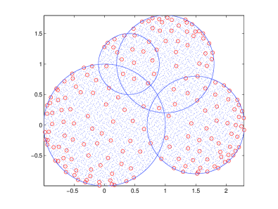
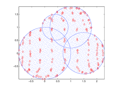
Figure 1: Extraction of 190 points for CATCHLS ($n=9$) from $M\approx 5600$ Halton points on the union of 4 disks: $C_{ratio}=M/m\approx 29$; top: by NonNegative Least Squares as in (5); bottom: by Linear Programming as in (6).

2.1 From the discrete to the continuum

In what follows we study situations where the sampling sets are discrete models of “continuous” compact sets, in the framework of polynomial approximation. In particular, we have in mind the case where $K$ is the closure of a bounded open subset of $\mathbb{R}^{d}$ (or of a bounded open subset of a lower-dimensional manifold in the induced topology, such as a subarc of the circle in $\mathbb{R}^{2}$ or a subregion of the sphere in $\mathbb{R}^{3}$). The so-called “Jackson compacts”, that are compact sets where a Jackson-like inequality holds, are of special interest, since there the best uniform approximation error $E_{n}(f)$ can be estimated by the regularity of $f$; cf. [24].

Such a connection with the continuum has already been exploited in the previous sections, namely on the right-hand side of the LS error estimates, e.g. in (21) and (29). Now, to get a connection also on the left-hand side, we should give some structure to the discrete sampling set $X$. We shall work within the theory of polynomial meshes, introduced in [7] and later developed by various authors; cf., e.g., [3, 4, 6, 14, 22] and the references therein.

We recall that a weakly admissible polynomial mesh of a compact set $K$ (or of a compact subset of a manifold) in $\mathbb{R}^{d}$ (we restrict here to the real case), is a sequence of finite subsets $X_{n}\subset K$ such that

$$\|p\|_{L^{\infty}(K)}\leq C_{n}\,\|p\|_{\ell^{\infty}(X_{n})}\;,\;\forall p\in\mathbb{P}_{n}^{d}(K)\;,$$ (33)

where $C_{n}=\mathcal{O}(n^{\alpha})$, $M_{n}=\mbox{card}(X_{n})=\mathcal{O}(n^{\beta})$, with $\alpha\geq 0$, and $\beta\geq d$. Indeed, since $X_{n}$ is automatically $\mathbb{P}_{n}^{d}(K)$-determining, then $M_{n}\geq N=\mbox{dim}(\mathbb{P}_{n}^{d}(K))=\mbox{dim}(\mathbb{P}_{n}^{d}(X_{n}))$. In the case where $\alpha=0$ (i.e., $C_{n}\leq C$) we speak of an admissible polynomial mesh, and such a mesh is termed optimal when $\mbox{card}(X_{n})=\mathcal{O}(N)$.

Polynomial meshes have interesting computational features (cf. [6]), e.g.

• extension by algebraic transforms, finite union and product

• contain computable near optimal interpolation sets [4, 5]

• are near optimal for uniform LS approximation, namely [7, Thm. 1]

  $$\|\mathcal{L}_{n}\|=\sup_{f\in C(K),\,f\neq 0}\frac{\|\mathcal{L}_{n}f\|_{L^{\infty}(K)}}{\|f\|_{L^{\infty}(K)}}\leq C_{n}\,\sqrt{M_{n}}\;,$$ (34)

  where $\mathcal{L}_{n}$ is the $\ell^{2}(X_{n})$-orthogonal projection operator $C(K)\to\mathbb{P}_{n}^{d}(K)$.

To prove (34), we can write the chain of inequalities

$$\|\mathcal{L}_{n}f\|_{L^{\infty}(K)}\leq C_{n}\,\|\mathcal{L}_{n}f\|_{\ell^{\infty}(X_{n})}\leq C_{n}\,\|\mathcal{L}_{n}f\|_{\ell^{2}(X_{n})}$$

$$\leq C_{n}\,\|f\|_{\ell^{2}(X_{n})}\leq C_{n}\,\sqrt{M_{n}}\,\|f\|_{\ell^{\infty}(X_{n})}\leq C_{n}\,\sqrt{M_{n}}\,\|f\|_{L^{\infty}(K)}\;,$$ (35)

where we have used the polynomial inequality (33) and the fact that $\mathcal{L}_{n}f$ is a discrete orthogonal projection. From (34) we get in a standard way the uniform error estimate

$$\|f-\mathcal{L}_{n}f\|_{L^{\infty}(K)}\leq\left(1+\|\mathcal{L}_{n}\|\right)\,E_{n}(f)\leq\left(1+C_{n}\,\sqrt{M_{n}}\right)\,E_{n}(f)\;,$$ (36)

valid for every $f\in C(K)$.

These properties show that polynomial meshes are good models of multivariate compact sets, in the context of polynomial approximation. Unfortunately, several computable meshes have high cardinality.

In [7, Thm. 5] it has been proved that admissible polynomial meshes can be constructed in any compact set satysfying a Markov polynomial inequality with exponent $r$, but these have cardinality $\mathcal{O}(n^{rd})$. For example, $r=2$ on convex compact sets with nonempty interior. Construction of optimal admissible meshes has been carried out for compact sets with various geometric structures, but still the cardinality can be very large already for $d=2$ or $d=3$, for example on polygons/polyhedra with many vertices, or on star-shaped domains with smooth boundary; cf., e.g., [14, 23].

As already observed, in the applications of LS approximation it is very important to reduce the sampling cardinality, especially when the sampling process is difficult or costly. Thus we may think to apply CATCH subsampling to polynomial meshes, in view of CATCHLS approximation, as in the previous section. In particular, it results that we can substantially keep the uniform approximation features of the polynomial mesh. We give the main result in the following

Proposition 3

Let $X_{n}$ be a polynomial mesh (cf. (33)) and let the assumptions of Proposition 2 be satisfied with $X=X_{n}$.

Then, the following estimate hold

$$\|\mathcal{L}_{n}^{c}\|=\sup_{f\in C(K),\,f\neq 0}\frac{\|\mathcal{L}_{n}^{c}f\|_{L^{\infty}(K)}}{\|f\|_{L^{\infty}(K)}}\leq C_{n}\,\sqrt{M_{n}}\,\beta_{M_{n}}(\varepsilon)\;,$$ (37)

provided that $\varepsilon\sqrt{M_{n}}<1$, where $\mathcal{L}_{n}^{c}f$ is the least squares polynomial at the Caratheodory-Tchakaloff points $T_{2n}\subseteq X_{n}$. Moreover,

$$\|p\|_{L^{\infty}(K)}\leq C_{n}\,\sqrt{M_{n}}\,\beta_{M_{n}}(\varepsilon)\,\|p\|_{\ell^{\infty}(T_{2n})}\;,\;\;\forall p\in\mathbb{P}_{n}^{d}(K)\;.$$ (38)

Proof. To prove (37), we can write the estimates

$$\|\mathcal{L}_{n}^{c}f\|_{L^{\infty}(K)}\leq C_{n}\,\|\mathcal{L}_{n}^{c}f\|_{\ell^{\infty}(X_{n})}\leq C_{n}\,\|\mathcal{L}_{n}^{c}f\|_{\ell^{2}(X_{n})}$$

$$\leq C_{n}\,\alpha_{M_{n}}(\varepsilon)\,\|\mathcal{L}_{n}^{c}f\|_{\ell^{2}_{\boldsymbol{w}}(T_{2n})}\leq C_{n}\,\alpha_{M_{n}}(\varepsilon)\,\|f\|_{\ell^{2}_{\boldsymbol{w}}(T_{2n})}\;,$$

using the first estimate in (27) for $p=\mathcal{L}_{n}^{c}f$ and the fact that $\mathcal{L}_{n}^{c}f$ is a discrete orthogonal projection, and then conclude by (30) applied to $f$.

Concerning (38), we can write

$$\|p\|_{L^{\infty}(K)}\leq C_{n}\,\|p\|_{\ell^{\infty}(X_{n})}\leq C_{n}\,\|p\|_{\ell^{2}(X_{n})}\;,$$

and then apply (27) to $p$.$\;\;\;\;\;\square$

By Proposition 3 and (28), we have that the (estimate of) the uniform norm of the CATCHLS operator has substantially the same size of (34), as long as $\varepsilon\sqrt{M_{n}}\ll 1$. On the other hand, inequality (38) with $\varepsilon=0$ says that

• the $2n$-deg CATCH points of a polynomial mesh are a polynomial mesh

  $$\|p\|_{L^{\infty}(K)}\leq C_{n}\,\sqrt{M_{n}}\,\|p\|_{\ell^{\infty}(T_{2n})}\;,\;\;\forall p\in\mathbb{P}_{n}^{d}(K)\;.$$ (39)

Moreover, (38) shows that such CATCH points, computed in finite-precision arithmetic, are still a polynomial mesh in the degree range where $\varepsilon\sqrt{M_{n}}\ll 1$. For a discussion of the consequences of (39) in the theory of polynomial meshes see [31].

In order to make an example, in Figure 2 we consider the (high cardinality) optimal polynomial mesh constructed on a smooth convex set ($C^{2}$ boundary), by the rolling ball theorem as described in [23] (the set boundary corresponds to a level curve of the quartic $x^{4}+4y^{4}$). The CATCH points have been computed by NNLS as in (5), and the LS and CATCHLS uniform operator norms have been numerically estimated on a fine control mesh via the corresponding discrete reproducing kernels, as discussed in [6, §2.1]. In Figure 2-bottom, we see that the CATCHLS operator norm is close to the LS operator norm, as we could expect from (34) and (37), which however turn out to be large overestimates of the actual norms.

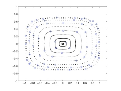
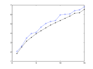
Figure 2: Top: polynomial mesh and extracted CATCH points on a smooth convex set ($n=5$, $C_{ratio}=971/66\approx 15$); bottom: numerically evaluated LS $(\ast)$ and CATCHLS $(\circ)$ uniform operator norms, for degree $n=1,\dots,15$.

References

- [1] G. Berschneider and Z. Sasvri, On a theorem of Karhunen and related moment problems and quadrature formulae, Spectral theory, mathematical system theory, evolution equations, differential and difference equations, 173–187, Oper. Theory Adv. Appl., 221, Birkhäuser/Springer Basel AG, Basel, 2012.
- [2] L. Bittante, S. De Marchi and G. Elefante, A new quasi-Monte Carlo technique based on nonnegative least-squares and approximate Fekete points, Numer. Math. Theory Methods Appl., to appear.
- [3] T. Bloom, L. Bos, J.-P. Calvi and N. Levenberg, Polynomial interpolation and approximation in , Ann. Polon. Math. 106 (2012), 53–81.
- [4] L. Bos, J.-P. Calvi, N. Levenberg, A. Sommariva and M. Vianello, Geometric Weakly Admissible Meshes, Discrete Least Squares Approximation and Approximate Fekete Points, Math. Comp. 80 (2011), 1601–1621.
- [5] L. Bos, S. De Marchi, A. Sommariva and M. Vianello, Computing multivariate Fekete and Leja points by numerical linear algebra, SIAM J. Numer. Anal. 48 (2010), 1984–1999.
- [6] L. Bos, S. De Marchi, A. Sommariva and M. Vianello, Weakly Admissible Meshes and Discrete Extremal Sets, Numer. Math. Theory Methods Appl. 4 (2011), 1–12.
- [7] J.P. Calvi and N. Levenberg, Uniform approximation by discrete least squares polynomials, J. Approx. Theory 152 (2008), 82–100.
- [8] C. Caratheodory, ber den Variabilittsbereich der Fourierschen Konstanten von positiven harmonischen Funktionen, Rend. Circ. Mat. Palermo 32 (1911), 193–217.
- [9] M. Conforti, G. Cornuéjols and G. Zambelli, Integer programming, Graduate Texts in Mathematics 271, Springer, Cham, 2014.
- [10] R.E. Curto and L.A. Fialkow, A duality proof of Tchakaloff’s theorem. J. Math. Anal. Appl. 269 (2002), 519–532.
- [11] S. Foucart and H. Rahut, A Mathematical Introduction to Compressive Sensing, Birkhäuser, 2013.
- [12] I. Griva, S.G. Nash and A. Sofer, Linear and Nonlinear Optimization, 2nd Edition, SIAM, 2009.
- [13] D. Huybrechs, Stable high-order quadrature rules with equidistant points, J. Comput. Appl. Math. 231 (2009), 933–947.
- [14] A. Kroó, On optimal polynomial meshes, J. Approx. Theory 163 (2011), 1107–1124.
- [15] C.L. Lawson and R.J. Hanson, Solving least squares problems. Revised reprint of the 1974 original, Classics in Applied Mathematics 15, SIAM, Philadelphia, 1995.
- [16] C. Litterer and T. Lyons, High order recombination and an application to cubature on Wiener space, Ann. Appl. Probab. 22 (2012), 1301–1327.
-
[17]
MATLAB, online documentation and manual (2016), available
at:
http://www.mathworks.com. - [18] G. Migliorati and F. Nobile, Analysis of discrete least squares on multivariate polynomial spaces with evaluations at low-discrepancy point sets, J. Complexity 31 (2015), 517–542.
-
[19]
GNU Octave, online documentation and manual (2016),
avalable at:
https://www.gnu.org/software/octave. - [20] F. Piazzon, A. Sommariva and M. Vianello, Quadrature of Quadratures: Compressed Sampling by Tchakaloff Points, poster presented at the 4th Dolomites Workshop on Constructive Approximation and Applications (DWCAA16), Alba di canazei (Trento, Italy), Sept. 2016; available online at: http://events.math.unipd.it/dwcaa16/?q=node/6.
- [21] F. Piazzon, A. Sommariva and M. Vianello, catchpts: a Matlab/Octave code for Caratheodory-Tchakaloff compression of multivariate discrete measures via Linear or Quadratic Programming, Nov. 2016, available online at: www.math.unipd.it/~marcov/CAAsoft.html.
- [22] F. Piazzon and M. Vianello, Small perturbations of polynomial meshes, Appl. Anal. 92 (2013), 1063–1073.
- [23] F. Piazzon and M. Vianello, Constructing optimal polynomial meshes on planar starlike domains, Dolomites Res. Notes Approx. DRNA 7 (2014), 22–25.
- [24] W. Pleśniak, Multivariate Jackson Inequality, J. Comput. Appl. Math. 233 (2009), 815–820.
- [25] E.K. Ryu and S.P. Boyd, Extensions of Gauss quadrature via linear programming, Found. Comput. Math. 15 (2015), 953–971.
-
[26]
M. Slawski, Nonnegative least squares: comparison of
algorithms (paper and code), available online at:
https://sites.google.com/site/slawskimartin/code. - [27] I.H. Sloan, Interpolation and Hyperinterpolation over General Regions, J. Approx. Theory 83 (1995), 238–254.
- [28] A. Sommariva and M. Vianello, Compression of multivariate discrete measures and applications, Numer. Funct. Anal. Optim. 36 (2015), 1198–1223.
- [29] V. Tchakaloff, Formules de cubatures mécaniques à coefficients non négatifs. (French) Bull. Sci. Math. 81 (1957), 123–134.
- [30] M. Tchernychova, “Caratheodory” cubature measures, Ph.D. dissertation in Mathematics (supervisor: T. Lyons), University of Oxford, 2015.
- [31] M. Vianello, Compressed sampling inequalities by Tchakaloff’s theorem, Math. Inequal. Appl. 19 (2016), 395–400.