The hot Jupiter of the magnetically-active weak-line T Tauri star V830 Tau

Abstract

We report results of an extended spectropolarimetric and photometric monitoring of the weak-line T Tauri star V830 Tau and its recently-detected newborn close-in giant planet. Our observations, carried out within the MaTYSSE programme, were spread over 91 d, and involved the ESPaDOnS and Narval spectropolarimeters linked to the 3.6-m Canada-France-Hawaii, the 2-m Bernard Lyot and the 8-m Gemini-North Telescopes. Using Zeeman-Doppler Imaging, we characterize the surface brightness distributions, magnetic topologies and surface differential rotation of V830 Tau at the time of our observations, and demonstrate that both distributions evolve with time beyond what is expected from differential rotation. We also report that near the end of our observations, V830 Tau triggered one major flare and two weaker precursors, showing up as enhanced red-shifted emission in multiple spectral activity proxies.

With 3 different filtering techniques, we model the radial velocity (RV) activity jitter (of semi-amplitude 1.2 km s^-1) that V830 Tau generates, successfully retrieve the $68\pm 11$ m s^-1 RV planet signal hiding behind the jitter, further confirm the existence of V830 Tau b and better characterize its orbital parameters. We find that the method based on Gaussian-process regression performs best thanks to its higher ability at modelling not only the activity jitter, but also its temporal evolution over the course of our observations, and succeeds at reproducing our RV data down to a rms precision of 35 m s^-1. Our result provides new observational constraints on scenarios of star / planet formation and demonstrates the scientific potential of large-scale searches for close-in giant planets around T Tauri stars.

1 Introduction

Magnetic fields are thought to play a key role in the formation of stars and their planets (e.g., André et al., 2009; Baruteau et al., 2014), and for their subsequent evolution into maturity. For instance, large-scale fields of low-mass pre-main-sequence (PMS) stars, the so-called T Tauri stars (TTSs), are known to control and even trigger physical processes such as accretion, outflows and angular momentum transport, through which they mostly dictate the rotational evolution of TTSs (e.g., Bouvier et al., 2007; Frank et al., 2014). Large-scale fields of TTSs may also help newborn close-in giant planets to avoid falling into their host stars and survive the fast migration that accretion discs efficiently trigger, thanks to the magnetospheric gaps that they carve at the disc centre (e.g., Lin et al., 1996; Romanova & Lovelace, 2006). The recent discoveries (or candidate detections) of newborn close-in giant planets around T Tauri stars (van Eyken et al., 2012; Mann et al., 2016; Johns-Krull et al., 2016; Donati et al., 2016; David et al., 2016) render the study of the latter topic particularly attractive and timely.

Although first detected long ago (e.g., Johns-Krull et al., 1999; Johns-Krull, 2007), magnetic fields of TTSs are not yet fully characterized, neither for those still surrounded by their accretion discs (the classical T Tauri stars / cTTSs) nor for those whose discs have dissipated already (the weak-line T Tauri stars / wTTSs). Only recently were the field topologies of a dozen cTTSs unveiled (e.g., Donati et al., 2007; Hussain et al., 2009; Donati et al., 2010, 2013) thanks to the MaPP (Magnetic Protostars and Planets) Large Observing Programme on the 3.6 m Canada-France-Hawaii Telescope (CFHT) with the ESPaDOnS high-resolution spectropolarimeter (550 hr of clear time over semester 2008b to 2012b). This first exploration revealed for instance that large-scale fields of cTTSs can be either relatively simple or quite complex depending on whether the host star is largely convective or mostly radiative (Gregory et al., 2012; Donati et al., 2013); it also showed that these fields vary with time (e.g., Donati et al., 2011, 2012, 2013) and mimic those of mature stars with similar internal structures (Morin et al., 2008), suggesting a dynamo origin.

The ongoing MaTYSSE (Magnetic Topologies of Young Stars and the Survival of close-in giant Exoplanets) Large Programme, allocated at CFHT over semesters 2013a-2016b (510 hr) with complementary observations with the Narval spectropolarimeter on the 2-m Télescope Bernard Lyot (TBL) at Pic du Midi in France (450 hr, allocated) and with the HARPS spectropolarimeter at the 3.6-m ESO Telescope at La Silla in Chile (135 hr, allocated), is carrying out the same kind of magnetic exploration on a few tens of wTTSs (Donati et al., 2014, 2015, hereafter D14, D15). MaTYSSE also aims at probing the potential presence of newborn close-in giant exoplanets (hot Jupiters / hJs) at an early stage of star / planet formation; it recently succeeded at detecting the youngest such body orbiting only 0.057 au (or 6.1 stellar radii) away from the 2 Myr wTTS V830 Tau (Donati et al., 2016, hereafter D16), strongly suggesting that disc migration is a viable and likely efficient mechanism for generating hJs.

In this new paper, we revisit the latest MaTYSSE data set collected on V830 Tau, including extended observations from early 2016 that follow the late 2015 ones from which V830 Tau b was detected, as well as contemporaneous photometry secured at the Crimean Astrophysical Observatory (CrAO). After briefly documenting these additional data (Sec. 2), we apply Zeeman-Doppler Imaging (ZDI) to both subsets to accurately model the surface features and large-scale magnetic fields generating the observed activity (Sec. 3). This modelling is then used to predict the activity jitter and retrieve the planet signature using two complementary methods, yielding results in agreement with a third completely independent technique based on Gaussian-process regression (e.g., Haywood et al., 2014; Rajpaul et al., 2015) and with those of D16 (Sec. 4). We finally summarize our results and stress how MaTYSSE-like explorations can unlock current limitations in our understanding of how giant planets and planetary systems form (Sec. 5).

2 Spectropolarimetric and photometric observations of V830 Tau

Following our intensive campaign in late 2015 (D16), V830 Tau was re-observed from 2016 Jan 14 to Feb 10, using again ESPaDOnS at the CFHT, its clone Narval at the TBL, and ESPaDOnS coupled to Gemini-North through the GRACES fiber link (Chene et al., 2014). ESPaDOnS and Narval collect spectra covering 370 to 1,000 nm at a resolving power of 65,000 (Donati, 2003). A total of 15, 6 and 6 spectra were respectively collected with ESPaDOnS, Narval and ESPaDOnS/GRACES, at a daily rate from Jan 14 to 30 and more sparsely afterwards. ESPaDOnS and NARVAL were used in spectropolarimetric modes, with all collected spectra consisting of a sequence of 4 individual subexposures (of duration 690 and 1200 s each for ESPaDOnS and Narval respectively) recorded in different polarimeter configurations to allow the removal of all spurious polarisation signatures at first order. ESPaDOnS/GRACES spectra were collected in spectroscopic “star only” mode, with a resolution similar to that of all other spectra, and consist of single 300 s observations. All raw frames are processed with the reference pipeline Libre ESpRIT implementing optimal extraction and radial velocity (RV) correction from telluric lines, yielding a typical rms RV precision of 20–30 m s^-1 (Moutou et al., 2007; Donati et al., 2008). Least-Squares Deconvolution (LSD, Donati et al., 1997) was applied to all spectra, using the same line list as in our previous studies (D15, D16). The full journal of observations is presented in Table 1.

Rotational and orbital cycles of V830 Tau (denoted $r$ and $o$ in the following equations) are computed from Barycentric Julian Dates (BJDs) according to the ephemerides:

BJD (d) $$= 2,457,011.80+2.741r$$ (1)

BJD (d) $$= 2,457,360.52+4.93o$$ (2)

in which the photometrically-determined rotation periods $P_{\rm rot}$ and the orbital period $P_{\rm orb}$ of the hJ are set to 2.741 d and 4.93 d respectively (Grankin, 2013, D16). Whereas the initial Julian date of the first ephemeris is chosen arbitrarily, that of the second one coincides with the inferior conjunction (with the hJ in front).

As in our late-2015 data (D16), a few spectra (8 altogether, corresponding to cycles 1.347, 2.090, 2.692, 2.820, 3.068, 3.185, 3.914 and 4.135) were weakly affected by moonlight in the far blue wing of the spectral lines, due to the proximity of the moon (passing within Taurus in Dec and Jan) and / or to non-photometric conditions. To filter this contamination from our Stokes $I$ LSD profiles, we applied the dual-step method described in D16, specifically designed for this purpose and shown to be quite efficient at restoring the original RVs down to noise level (50 m s^-1 rms in our case, see Table 1).

Table 1: Journal of ESPaDOnS observations of V830 Tau collected in from 2016 Jan 14 to Feb 10. ESPaDOnS and Narval spectropolarimetric observations consist of sequences of 4 subexposures (each lasting 690 s and 1200 s respectively) whereas ESPaDOnS/GRACES exposures correspond to single (unpolarized) observations lasting 300 s each. Columns $1-5$ respectively list (i) the UT date of the observation, (ii) the instrument used, (iii) the corresponding UT time (at mid-exposure), (iv) the Barycentric Julian Date (BJD), and (v) the peak signal to noise ratio S/N (per 2.6 km s^-1 velocity bin) of each observation. Columns 6 and 7 respectively list the S/N in Stokes $I$ LSD profiles (per 1.8 km s^-1 velocity bin), and the rms noise level (relative to the unpolarized continuum level $I_{\rm c}$) in Stokes $V$ LSD profiles (whenever relevant). Columns 8 and 9 indicate the rotational $r$ and orbital $o$ cycles associated with each exposure (using the ephemerides given by Eq. 2). Columns 10–12 respectively give the raw and ZDI-filtered RVs $v_{\rm raw}$ and $v_{\rm fil}$, as well as the corresponding 1$\sigma$ error bars $\sigma_{\rm RV}$. No $v_{\rm fil}$ estimates are available for Jan 30 and Feb 10 spectra, affected by strong flares. The observation log of our late 2015 data can be found in D16 (Extended Data Table 1).

Date	Instrument	UT	BJD	S/N	$\hbox{S/N}_{\rm LSD}$	$\sigma_{\rm LSD}$	$r$	$o$	$v_{\rm raw}$	$v_{\rm fil}$	$\sigma_{\rm RV}$
(2016)		(hh:mm:ss)	(2,457,400+)			(0.01%)	(142+)	(8+)	(km/s)	(km/s)	(km/s)
Jan 14	ESPaDOnS	08:19:57	1.85135	150	1460	3.3	0.303	0.384	0.254	$-0.017$	0.049
Jan 15	ESPaDOnS	08:16:30	2.84889	150	1400	3.3	0.667	0.586	0.789	0.020	0.051
Jan 16	ESPaDOnS	08:34:49	3.86153	160	1480	2.9	1.036	0.791	$-0.287$	0.005	0.048
Jan 17	ESPaDOnS	05:02:34	4.71408	170	1470	2.9	1.347	0.964	$-0.008$	0.000	0.049
Jan 18	ESPaDOnS	07:32:40	5.81823	160	1420	3.1	1.750	1.188	$-0.380$	$-0.016$	0.050
Jan 19	ESPaDOnS	05:55:30	6.75069	170	1470	2.9	2.090	1.377	$-0.123$	$-0.092$	0.049
Jan 20	Narval	21:30:38	8.39998	90	1130	5.1	2.692	1.712	0.546	0.089	0.063
Jan 21	ESPaDOnS	05:55:40	8.75065	150	1440	3.3	2.820	1.783	$-1.013$	0.034	0.050
Jan 21	Narval	22:16:00	9.43141	100	1240	4.6	3.068	1.921	$-0.099$	0.035	0.058
Jan 22	ESPaDOnS	05:56:39	9.75126	140	1450	3.5	3.185	1.986	0.386	$-0.006$	0.049
Jan 23	ESPaDOnS	07:00:55	10.79581	160	1450	3.0	3.566	2.198	1.170	0.015	0.050
Jan 24	ESPaDOnS	05:57:09	11.75144	170	1450	3.0	3.914	2.392	$-1.258$	$-0.069$	0.049
Jan 24	Narval	20:25:57	12.35475	70	970	6.5	4.135	2.514	0.180	0.025	0.074
Jan 25	ESPaDOnS	07:23:59	12.81166	150	1470	3.4	4.301	2.607	0.284	$-0.011$	0.049
Jan 26	ESPaDOnS	06:59:05	13.79429	150	1420	3.5	4.660	2.806	0.840	$-0.011$	0.051
Jan 26	Narval	19:34:05	14.31857	90	1130	5.4	4.851	2.912	$-1.160$	0.039	0.064
Jan 27	ESPaDOnS	06:05:23	14.75691	170	1470	2.9	5.011	3.001	$-0.482$	0.009	0.049
Jan 28	ESPaDOnS	06:05:42	15.75705	160	1440	3.1	5.376	3.204	$-0.176$	$-0.031$	0.050
Jan 29	ESPaDOnS	06:58:43	16.79378	150	1410	3.3	5.754	3.415	$-0.444$	$-0.036$	0.051
Jan 29	Narval	20:01:53	17.33762	80	1210	5.6	5.952	3.525	$-0.956$	0.011	0.059
Jan 30	Narval	20:15:57	18.34730	80	1190	6.1	6.321	3.730	0.000		0.060
Feb 04	GRACES	07:12:12	22.80262	140	1560		7.946	4.633	$-1.017$	$-0.005$	0.046
Feb 04	GRACES	07:18:12	22.80678	150	1560		7.948	4.634	$-0.978$	0.023	0.046
Feb 09	GRACES	07:16:45	27.80532	150	1470		9.771	5.648	$-0.621$	$-0.019$	0.049
Feb 09	GRACES	07:22:39	27.80941	150	1470		9.773	5.649	$-0.628$	$-0.010$	0.049
Feb 10	GRACES	05:21:11	28.72497	160	1600		10.107	5.835	$-0.653$		0.045
Feb 10	GRACES	05:27:05	28.72907	160	1590		10.108	5.836	$-0.647$		0.045

Contemporaneous BVR_JI_J photometric observations were also collected from the CrAO 1.25 m telescope (see Table 2), showing that V830 Tau exhibited significantly larger brightness fluctuations than a year before (D15), with a full amplitude of 0.28 mag and a period of $2.7424\pm 0.0014$ d (compatible within error bars with the average periods of Grankin, 2013, used to phase our spectroscopic data, see Eq. 2).

Table 2: Journal of contemporaneous CrAO multicolour photometric observations of V830 Tau collected from 2015 Oct 30 to 2016 Mar 15, respectively listing the Heliocentric Julian Date (HJD) of the observation, the measured ${\rm V}$ magnitude, ${\rm B-V}$, ${\rm V-R_{\rm J}}$ and ${\rm V-I_{\rm J}}$ Johnson photometric colours, and the corresponding rotational cycle (using again the ephemerides of Eq. 2). The middle line separates observations collected in 2015 and 2016. The typical 1$\sigma$ error bar on ${\rm V}$ is 20 mmag.

HJD	${\rm V}$	${\rm B-V}$	${\rm V-R_{\rm J}}$	${\rm V-I_{\rm J}}$	$r$
(2,457,300+)	(mag)	(mag)	(mag)	(mag)	(114+)
26.4574	12.410		1.339	2.182	0.797
28.5085	12.378			2.242	1.545
30.6098	12.322	1.375	1.325	2.151	2.311
31.5960	12.474	1.413	1.341	2.231	2.671
32.5964	12.267	1.349		2.143	3.036
40.5358	12.307		1.340	2.165	5.933
44.4530	12.321		1.321	2.146	7.362
47.5027	12.342		1.307	2.162	8.475
47.5524	12.367		1.335	2.180	8.493
73.3208	12.317		1.319	2.161	17.894
73.5082	12.261		1.305	2.130	17.962
74.2657	12.268		1.310	2.128	18.238
91.3173	12.281		1.307	2.122	24.459
101.2599	12.199		1.282	2.094	28.087
105.2842	12.356		1.319	2.155	29.555
112.2820	12.244		1.284	2.113	32.108
118.2602	12.306		1.339	2.160	34.289
127.2569	12.362		1.325	2.165	37.571
129.2079	12.252		1.296	2.105	38.283
141.2201	12.413		1.343	2.204	42.665
142.2211	12.210		1.301	2.106	43.031
153.2096	12.219		1.297	2.106	47.040
156.2255	12.196		1.288	2.094	48.140
158.2696	12.329		1.332	2.148	48.886
163.2378	12.425		1.322	2.217	50.698

We note that V830 Tau features emission in various spectral activity proxies, as expected from its youth and fast rotation. More specifically, Balmer lines and in particular H${\alpha}$, are in emission, as well as the central core of the Ca ii infrared triplet (IRT) lines, with typical equivalent widths of 85 and 16 km s^-1 for H${\alpha}$ and the Ca ii IRT emission core respectively. The He i $D_{3}$ line is most of the time quite shallow, with an average equivalent width of 5 km s^-1.

In 2016 however, we detected several flares of V830 Tau, showing up as enhanced red-shifted emission in all activity proxies including He i, a reliable proxy whose high excitation potential makes it possible to separate flares from phases of enhanced chromospheric activity (e.g., Montes et al., 1997). The most intense flare occurred on Feb 10 during our last pair of observations (cycles 10.107 and 10.108), when H${\alpha}$, Ca ii IRT and He i emission reach equivalent widths of 280, 32 and 25 km s^-1 and feature large red-shifts of 15–35 km s^-1 (with respect to the stellar rest frame, shifted from the Barycentric rest frame by $\simeq$17 km s^-1) and asymmetric profiles (with a conspicuous red tail for H${\alpha}$, see Fig. 1, and He i). We note that one of our photometric measurements was secured just after this large flare (at rotation cycle 152.283, or 10.283 in the reference frame of Table 1). At this time, the star was observed to be 54 mmag (i.e., 2.7$\sigma$) brighter than 4 rotation cycles earlier at almost the same phase (cycle 148.289, see Table 2). This shows that even the largest flare of our run was barely detectable in the light curve, to the point that it is not even clear which of the two photometric measurements at this phase deviates most from the bulk of our data points (see Sec. 3).

A weaker flare was detected 10.3 d earlier on Jan 30 (cycle 6.321), with activity proxies exhibiting similar albeit less drastic characteristics, e.g., He i emission with an equivalent width of 11 km s^-1 and a redshift of $\simeq$20 km s^-1 (with respect to the stellar rest frame, or $\simeq$10 km s^-1 with respect to the average velocity of the He i line). A third flare was recorded on Jan 26 (cycle 4.851), mostly in H${\alpha}$ (with an equivalent width reaching 122 km s^-1), but short enough to be seen only with Narval, but neither a few hours before (cycle 4.660) nor later (cycle 5.011) with ESPaDOnS; this flare has only mild He i characteristics however, with an equivalent width only slightly above average and no significant redshift (with respect to the average line velocity).

The 3 Stokes $I$ spectra corresponding to the 2 first flares turned out to yield discrepant RV estimates (with excess blue-shifts of order 0.3 km s^-1), most likely as a result of flaring, and were removed from the subsequent modelling (see Secs. 3 and 4). The Stokes $V$ spectrum associated with the second flare compares well with those collected at similar phases but previous cycles (0.303, 4.301), suggesting that it was largely unaffected by the flare and thus used for magnetic imaging (see Sec. 3). The Stokes $I$ (and $V$) spectra corresponding to the third, milder, flare, yielding an RV estimate consistent with those from the two unperturbed ESPaDOnS spectra bracketing the flare, were also kept in the sample.

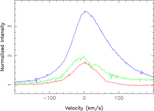
Figure 1: H${\alpha}$ profiles of V830 Tau on 2016 Jan 17 (cycle 1.347, red line), Feb 10 (cycle 10.107, blue) and Jan. 30 (cycle 6.321, green). A red component / tail is clearly present in the latter two profiles (recorded during a flare) while absent in the first one (more typical of V830 Tau).

             

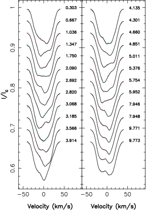
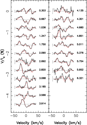
Figure 2: Maximum-entropy fit (thin red line) to the observed (thick black line) Stokes $I$ (left panel) and Stokes $V$ (right panel) LSD photospheric profiles of V830 Tau in early 2016. (The red and black lines almost perfectly overlap for Stokes $I$ LSD profiles.) Stokes $I$ LSD profiles prior to their filtering from lunar contamination (in the far blue wing) are also shown (cyan line). Rotational cycles and 3$\sigma$ error bars (for Stokes $V$ profiles) are also shown next to each profile.

3 Tomographic modelling of surface features, magnetic fields and activity

We applied ZDI to both our late-2015 and early-2016 sets of phase-resolved Stokes $I$ and $V$ LSD profiles, keeping them separate from each other in a first step. ZDI is a tomographic technique inspired from medical imaging, with which distributions of brightness features and magnetic fields at the surfaces of rotating stars can be reconstructed from time-series of high-resolution spectropolarimetric observations (Brown et al., 1991; Donati & Brown, 1997; Donati, 2001; Donati et al., 2006). Technically speaking, ZDI follows the principles of maximum-entropy image reconstruction, and iteratively looks for the image with lowest information content that fits the data at a given $\chi^{2}$ level. By working out the amount of latitudinal shearing that surface maps are subject to as a function of time, ZDI can also infer an estimate of differential rotation at photospheric level (Donati & Collier Cameron, 1997; Donati et al., 2003).

For this study, we used the latest implementation of ZDI, where the large-scale field is decomposed into its poloidal and toroidal components, both expressed as spherical harmonics expansions (Donati et al., 2006), and where the brightness distribution incorporates both cool spots and warm plages (D14, D15, D16). The local Stokes $I$ and $V$ profiles are computed using Unno-Rachkovsky’s analytical solution to the polarized radiative transfer equations in a Milne-Eddington model atmosphere, taking into account the local brightness and magnetic field; these local profiles are then integrated over the visible hemisphere to derive the synthetic profiles of the rotating star, to be compared with our observations. This computation scheme provides a reliable description of how line profiles are distorted in the presence of magnetic fields (including magneto-optical effects, e.g., Landi degl’Innocenti & Landolfi, 2004).

In this new paper, we assume for V830 Tau the same parameters as in our previous studies in particular an inclination of the rotation axis to the line of sight $i$ equal to $55\pm 10$^∘ and a line-of-sight-projected equatorial rotation velocity $v\sin i$ equal to $30.5\pm 0.5$ km s^-1 (D15, D16). We recall that the inclination angle $i$ is derived both from the measured stellar parameters (see Sec. 3 of D15) and by minimizing the information content of reconstructed images, with a typical error bar of order 10^∘. We further assume that the (weak) surface differential rotation of V830 Tau is as derived by D16 from our late 2015 data alone, before revisiting the subject using the whole data set in Sec. 3.2. The parameters of V830 Tau used in our study are summarized in Table 3.

Table 3: Summary of the main parameters of V830 Tau, with references as mentioned whenever appropriate (G13 and R12 stand for Grankin 2013 and Rodríguez et al. 2012).

Parameter	Value	Reference
$M_{\star}$ (${\rm M}_{\odot}$)	$1.00\pm 0.05$	D15
$R_{\star}$ (${\rm R}_{\odot}$)	$2.0\pm 0.2$	D15
age (Myr)	$\simeq$2.2	D15
$P_{\rm rot}$ (d)	2.741	G13
BJD0	2,457,011.80	D15
$\Omega_{\rm eq}$ (rad d-1)	$2.29525\pm 0.00020$	D16
$d\Omega$ (rad d-1)	$0.0172\pm 0.0014$	D16
$i$ (∘)	$55\pm 10$	D15
$v\sin i$ (km s-1)	$30.5\pm 0.5$	D15
distance (pc)	$150\pm 5$	R12
$T_{\rm eff}$(K)	$4250\pm 50$	D15

3.1 Brightness and magnetic imaging

                               

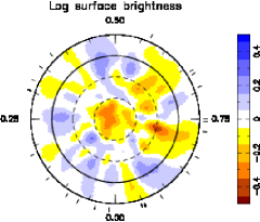
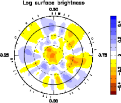
Figure 3: Maps of the logarithmic brightness (relative to the quiet photosphere), at the surface of V830 Tau in early 2016 (left) and late 2015 (right). Cool spots / bright plages show up as brown / blue features. The star is shown in flattened polar projection down to latitudes of $-30\hbox{${}^{\circ}$}$, with the equator depicted as a bold circle and parallels as dashed circles. Radial ticks around each plot indicate phases of observations.

          

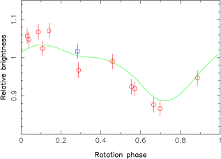
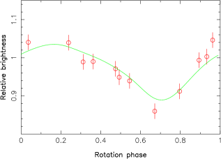
Figure 4: Brightness variations of V830 Tau in early 2016 (left) and late 2015 (right) as predicted from the tomographic modelling of our spectropolarimetric data (see Fig. 3, green line), compared with contemporaneous photometric observations in the ${\rm V}$ band (open symbols and 1$\sigma$ error bars of 20 mmag) at the 1.25-m CrAO telescope (see Table 2). The photometric measurement collected immediately after the large flare detected in our early 2016 spectroscopy data (see Sec. 2) is shown as an open blue square in the left panel.

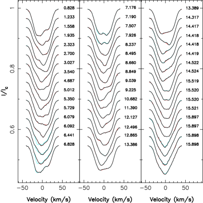
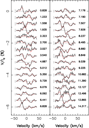
Figure 12: Same as Fig. 2 for our late 2015 observations.

In Fig. 2, we show our sets of Stokes $I$ and $V$ LSD profiles of V830 Tau from early 2016, along with the fit to the data. A similar plot is provided in Appendix A for our late-2015 data set (see Fig. 12, repeating Fig. 1 of D16 for Stokes $I$ profiles, and including Stokes $V$ profiles not previously shown in D16). The fit we obtain in both cases corresponds to a $\chi^{2}$ equal to the number of data points, i.e., to a unit $\chi^{2}_{\rm r}$ level (where $\chi^{2}_{\rm r}$ is simply taken here as $\chi^{2}$ divided by the number of data points, respectively equal to 1104 and 2208 for the early-2016 and late-2015 Stokes $I$ data sets, and to 966 and 1472 for the corresponding Stokes $V$ data sets). The initial $\chi^{2}_{\rm r}$ values, corresponding to input maps with null fields and no brightness features, are equal to 27 and 19 for the early-2016 and late-2015 data sets respectively, clearly demonstrating the overall success of ZDI at modelling the observed modulation of both Stokes $I$ and $V$ LSD profiles.

The reconstructed brightness maps of V830 Tau at both epochs are shown in Fig. 3. The two maps share obvious similarities and exhibit similar spottedness levels, i.e., $\simeq$13% of the stellar surface (7% and 6% for cool and warm features respectively). In particular, most cool spots and warm plages present in either maps are recovered at both epochs. One can also notice differential rotation shearing the brightness distribution between late 2015 and early 2016 (a time gap corresponding to 49 d or 18 rotation cycles), with equatorial and polar features being both shifted by a few % of a rotation cycle to smaller and larger phases respectively (implying a fast equator and a slow pole, in good quantitative agreement with D16). Some intrinsic temporal evolution beyond differential rotation may be visible in our images as well, with, e.g., the appearance of a warm equatorial plage at phase 0.08 in early 2016 that was not visible (or not as strong) in late 2015; however, even though phase coverage is fairly good in our case at both epochs, quantifying spot evolution by visually comparing images derived from differently sampled data sets is notoriously ambiguous and misleading. We come back on this point in Sec. 3.2.

We stress that the derived brightness images predict light curves that are in good agreement with our observations (see Fig. 4), even though these images were produced from our sets of LSD profiles only. Note the small temporal evolution in the predicted light curves between both epochs, that our photometric observations cannot confirm due to their limited sampling and precision. This further demonstrates that LSD profiles contain enough information to accurately predict the surface distribution of brightness features, and in particular those responsible of the RV activity jitter (see Sec. 4); on the opposite, it is quite obvious that photometric information is way too limited (even when better sampled and more precise) to infer complex spot distributions such as those we reconstruct for V830 Tau. It implies that jitter-filtering techniques based solely on photometry (e.g., Aigrain et al., 2012) are likely to yield poorer results, especially for moderate to fast rotators whose optical RV curves are much more sensitive than photometry to small features in surface brightness distributions.

The large-scale magnetic topologies we retrieve for V830 Tau at both epochs (see Fig. 5) are again very similar, with rms surface magnetic fluxes of 350 G, and resemble that found previously for this star (D15). As for the brightness maps, the main magnetic regions that we recover are visible at both epochs. More specifically, the field is found to be 90% poloidal, featuring a 340 G dipole field tilted at $22\pm 5$^∘ to the rotation axis towards phase $0.79\pm 0.03$ (in late 2015) and $0.88\pm 0.03$ (in early 2016), and that gathers 60% of the poloidal field energy. Weaker quadrupolar and octupolar components (of strength 100–150 G) and smaller-scale features are also present on V830 Tau, giving the field close to the stellar surface a more complex appearance than that of the dominating dipole. With a rms flux of $\simeq$110 G, the toroidal field is weak and of rather complex topology. The extrapolated large-scale magnetic topology (in the assumption of a potential field) is shown in Fig. 6 at both epochs.

           

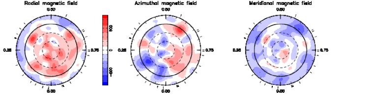
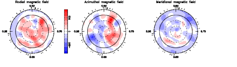
Figure 5: Maps of the radial (left), azimuthal (middle) and meridional (right) components of the magnetic field $\bf B$ at the surface of V830 Tau in early 2016 (top) and late 2015 (bottom). Magnetic fluxes in the color lookup table are expressed in G. The star is shown in flattened polar projection as in Fig. 3.

   

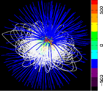
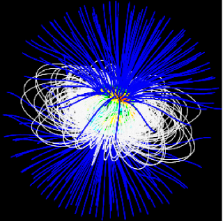
Figure 6: Potential extrapolations of the magnetic field reconstructed for V830 Tau in early 2016 (left) and late 2015 (right), as seen by an Earth-based observer at phase 0.10. Open and closed field lines are shown in blue and white respectively, whereas colors at the stellar surface depict the local values (in G) of the radial field (see left panels of Fig. 5). The source surface at which the field becomes radial is set at a distance of 4 $R_{\star}$, close to the corotation radius of V830 Tau (at which the Keplerian orbital period equals the stellar rotation period and beyond which field lines tend to open under the effect of centrifugal forces, Jardine 2004) but smaller than the Alfvén radius expected for a T Tauri star like V830 Tau ($>$6 $R_{\star}$, see Vidotto & Donati, 2016). Note how the high-latitude open-field regions slightly lag behind rotation between both epochs as a result of differential rotation.

As for the brightness maps, the magnetic images show evidence of a global differential rotation shear similar to that reported by D15, with equatorial regions (e.g., the strong negative azimuthal feature at phase 0.17) moving to slightly earlier phases from late 2015 to early 2016, and higher latitude regions (e.g., the positive radial field region at phase 0.05 and latitude 60^∘) moving to later phases at the same time. The increase in the phase towards which the dipole is tilted (0.79 and 0.88 in late 2015 and early 2016 respectively) comes as additional evidence that high latitudes (at which the dipole poles are anchored) are rotating more slowly than average, by typically 1 part in 200; this is further confirmed by the fact that the line-of-sight projected (longitudinal) magnetic fields (proportional to the first moment of the Stokes $V$ profiles, e.g., Donati et al., 1997, and most sensitive to the low-order components of the large-scale field) exhibit a recurrence timescale of $1.004\pm 0.003$ $P_{\rm rot}$, i.e. slightly longer than $P_{\rm rot}$ by a similar amount.

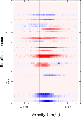
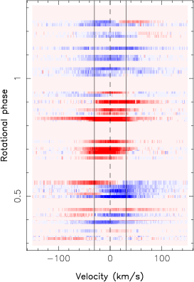
Figure 13: Dynamic spectra of H${\alpha}$ residual of V830 Tau in late 2016 (left) and early 2015 (right), with residuals computed with respect to the $\hbox{S/N}^{2}$-weighted mean over the whole observing run (after the removal of a few flaring spectra, see Sec. 2). Note how the phase of maximum H${\alpha}$ emission increases from 0.8 to 0.9 from late 2015 to early 2016. Red / blue means positive / negative residuals, with amplitudes ranging from –0.3 to 0.3 (in units of the continuum level), whereas the dashed and full vertical lines depict the line centre (in the stellar rest frame) and the stellar rotational broadening $v\sin i$.

We also report that the phase of maximum H${\alpha}$ emission of V830 Tau coincides, in both late 2015 and early 2016, with that of the high-latitude regions at which the dipole field is anchored; this is obvious from the dynamic spectra of the H${\alpha}$ residuals that we provide as an additional figure in the Appendix (see Fig. 13). A logical by-product is that H${\alpha}$ emission of V830 Tau, like its longitudinal field, is modulated by a period slightly longer than $P_{\rm rot}$, and equal to $1.004\pm 0.002$ $P_{\rm rot}$. From the solar analogy, one would have expected chromospheric emission to be minimum when open field lines point towards the observer, i.e., at phase 0.8–0.9 (see Fig. 6); this is however not what we observe, suggesting that the H${\alpha}$ emission we detect comes from regions close to (but not coinciding with) the strongest radial field regions that we reconstruct at high latitudes (see Fig. 5).

We also note apparent temporal evolution of the magnetic topology, with, e.g., the positive radial field region close to the equator at phase 0.33 growing much stronger between late 2015 and early 2016, though we caution again that a simple visual image comparison of individual features can be misleading.

     

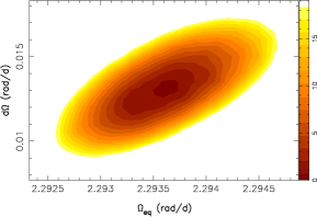
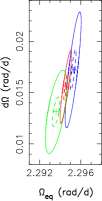
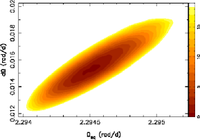
Figure 7: Variations of $\Delta\chi^{2}$ as a function of the differential rotation parameters $\Omega_{\rm eq}$ and $d\Omega$, derived from modelling our full set of Stokes $I$ (right) and $V$ (left) LSD profiles of V830 Tau at constant information content. A well defined paraboloid is observed in both cases, with the outer color contour tracing the 99.99% confidence interval (corresponding to a $\Delta\chi^{2}$  of 18.4 for the 2438 Stokes $V$ and 3312 Stokes $I$ data points). In both cases, the minimum $\chi^{2}_{\rm r}$ achieved (equal to 1.62 and 1.18 for Stokes $I$ and Stokes $V$ data respectively) is significantly larger than 1; this value is used to normalise $\chi^{2}$ before computing $\Delta\chi^{2}$ so as to account for intrinsic variability (affecting the brightness distribution and magnetic field of V830 Tau over the course of our 91-d run, see Sec 3.2) when estimating errors bars on differential rotation parameters. The values we obtain for these parameters are equal to $\hbox{$\Omega_{\rm eq}$}=2.29455\pm 0.00014$ rad d^-1 and $\hbox{$d\Omega$}=0.0156\pm 0.0009$ rad d^-1 for the Stokes $I$ data, and $\hbox{$\Omega_{\rm eq}$}=2.29360\pm 0.00025$ rad d^-1 and $\hbox{$d\Omega$}=0.0131\pm 0.0010$ rad d^-1 for the Stokes $V$ data. The middle plot emphasizes how the confidence intervals from both measurements compare with each other, and with that derived from the late-2015 Stokes $I$ LSD profiles only (D16). The 68.3% and 99.99% confidence intervals (dashed and full lines) are shown in green, red and blue for the full Stokes $V$, the full Stokes $I$ and the late-2015 Stokes $I$ data sets respectively.

3.2 Intrinsic variability and surface differential rotation

The most reliable way to assess whether intrinsic variability occurred at the surface of V830 Tau between late 2015 and early 2016 is to attempt modelling both data sets simultaneously with a unique brightness and magnetic topology, and see whether one can fit the full set to the same $\chi^{2}_{\rm r}$ level as that achieved for the individual sets (i.e., 1.0, see Sec. 3). We find that this is not possible, with a minimum achievable $\chi^{2}_{\rm r}$ of 1.62 and 1.18 for Stokes $I$ and Stokes $V$ data respectively (starting from initial $\chi^{2}_{\rm r}$ of 35 and 5); this confirms our previous suspicion that intrinsic variability occurred at the surface of V830 Tau throughout the 91 d (33 rotation cycles) of our observing campaign, and in particular over the 49 d shift between our two data sets. The global fit to the full data set we obtain nonetheless captures most of the observed line profile fluctuations, indicating that the intrinsic variability at work at the surface of V830 Tau remained moderate and local without altering the brightness and magnetic surface distributions too drastically; this further confirms our visual impression that images from both epochs shared obvious similarities.

Despite this intrinsic variability, we attempted to estimate differential rotation from our full data set. As in previous papers, we achieve this by assuming that the rotation rate at the surface of V830 Tau $\Omega(\theta)$ varies with latitude $\theta$ as $\sin^{2}\theta$ and depends on 2 main parameters, the rotation rate at the equator $\Omega_{\rm eq}$ and the difference in rotation rate $d\Omega$ between the equator and the pole (so that $\Omega(\theta)=\hbox{$\Omega_{\rm eq}$}-\hbox{$d\Omega$}\sin^{2}\theta$). Both parameters are derived by looking for the pair that minimizes the $\chi^{2}_{\rm r}$ of the fit to the data (at constant information content in the reconstructed image), whereas the corresponding error bars are computed from the curvature of the $\Delta\chi^{2}$ paraboloid at its minimum (Donati et al., 2003). ($\Delta\chi^{2}$ is defined as the $\chi^{2}$ increase with respect to the minimum $\chi^{2}$ in the map.) Results are shown in Fig. 7. The differential rotation we derive from our complete data set is slightly smaller (though still compatible at a $\simeq$3$\sigma$ level) than that inferred from the late-2015 Stokes $I$ LSD profiles only (D16). Despite the fact that this weakening is observed in both Stokes $I$ and $V$ data, we think that this small change likely results from intrinsic variability at the surface of V830 Tau.

Further evidence that high latitudes of V830 Tau are rotating more slowly than average (in agreement with the differential rotation pattern we recover) comes from the drift to later phases of the polar regions at which the large-scale dipole field component is anchored and where H${\alpha}$ emission is strongest.

4 Filtering the activity jitter and modelling the planet signal

We describe below the results of 3 independent techniques aimed at characterizing the RV signature of V830 Tau b from our data. The first 2 methods are those already outlined in D16 and used to detect V830 Tau b from the late-2015 data alone, that we now apply to both late-2015 and early-2016 data sets, with some modifications to account for the intrinsic variability between the 2 epochs (see Sec. 3.2). The third one follows the approach of Haywood et al. (2014) and Rajpaul et al. (2015), and uses Gaussian-process regression (GPR) to model activity directly from the raw RVs. The results obtained with each technique are described and compared in the following sections.

4.1 Modeling the planet signal from filtered RVs (ZDI #1)

The first technique consists in using the ZDI brightness images of Fig. 3 to predict the RV curves expected for V830 Tau at each epoch, and compare them with observed raw RVs. Modeled and raw RVs are both computed as the first order moment of Stokes $I$ LSD profiles (i.e., $\int(1-I(v))vdv/\int(1-I(v))dv$ where $v$ is the radial velocity across the line profile) while error bars on raw RVs are derived from those propagated from the observed spectra to the Stokes $I$ LSD profiles (and checked for consistency through simulated data sets as in D16); activity-filtered RVs are then derived by simply subtracting the modelled RVs from the observed ones (D16, see Table 1). Even though the intrinsic variability observed at the surface of V830 Tau is only moderate (see Sec. 3.2), using a specific ZDI map for each data subset (i.e., late 2015 and early 2016) is essential to obtain precise filtered RVs; using a single image for both subsets and ignoring the temporal evolution of the surface brightness distribution between the two epochs (beyond that caused by differential rotation) significantly degrades the quality of the modelling and therefore the precision of the filtered RVs.

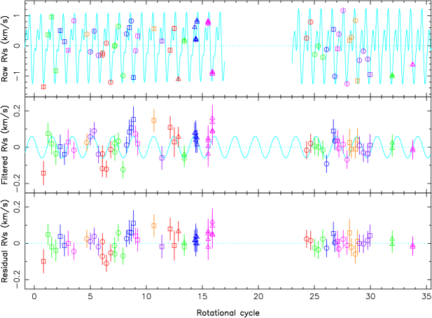
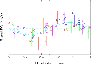
Figure 8: Top panel: Raw (top), filtered (middle) and residual (bottom) RVs of V830 Tau (open symbols and 1$\sigma$ error bars, with circles, squares and triangles depicting ESPaDOnS, NARVAL and ESPaDOnS/GRACES data, and colors coding rotation cycles). The raw RVs exhibit a semi-amplitude of 1.2 km s^-1 and a rms dispersion of 0.65 km s^-1 throughout the whole run. (Rotation cycles of the 2016 data are shifted by $+24$ in this plot with respect to their values in Table 1 and Fig. 2). The RV jitter predicted by ZDI at both epochs, as well as the best sine fit to the filtered RVs, are added in the top and middle plots (cyan lines). Note how the jitter model changes between late 2015 and early 2016, and how both of them slowly evolve with time as a result of differential rotation. The rms dispersion of the residual RVs is 44 m s^-1, in agreement with our measurement errors (see Table 1). Bottom panel: Activity-filtered RVs phase-folded on the planet orbital period. The fit to the data is only marginally better with an eccentric orbit (dashed line) than with a circular one (solid line).

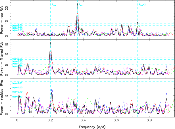
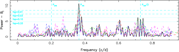
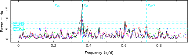
Figure 9: Top panel: Lomb-Scargle periodograms of the raw (top), filtered (middle) and residual RVs (bottom) shown in Fig 8. The black line is for the full set, while the dashed red, green, blue and pink lines are for the late-2015, the early-2016, the even, and the odd points only. The stellar rotation period, its first harmonic and the planet orbital period are depicted with vertical dashed lines. The horizontal dotted and dashed lines trace the 33%, 10%, 3% and 1% FAP levels. The planet signal in the filtered RVs is detected in the full set with a FAP level $<10^{-5}$. Middle panel: Periodogram of the longitudinal magnetic field, a reliable activity proxy (Haywood et al., 2016), featuring a clear peak at the stellar rotation period but no power at the planet orbital period. Bottom panel: Same as middle panel for the H${\alpha}$ emission.

The results we obtain are shown in Fig. 8 for the raw, filtered and residual RVs, and in Fig. 9 for the corresponding periodograms. The planet RV signal is very clearly detected in the filtered RVs, with a false-alarm probability (FAP) lower than $10^{-5}$. The $\chi^{2}$ decrease that we obtain with our fit to the filtered RVs (with respect to a case with no planet) is about 36 (for 72 RV points and 4 degrees of freedom), suggesting a similarly-low FAP value of $<$10^-6. The corresponding curve features a semi-amplitude equal to $K=60\pm 10$ m s^-1 and an orbital period of $\hbox{$P_{\rm orb}$}=4.97\pm 0.03$ d, in agreement with the estimates of D16 ($K=75\pm 12$ m s^-1 and $\hbox{$P_{\rm orb}$}=4.93\pm 0.05$ d). Fitting a Keplerian orbit through the data marginally improves the fit, but the derived eccentricity ($0.21\pm 0.15$) is not measured with enough precision to be reliable (Lucy & Sweeney, 1971); it confirms at least that V830 Tau b is close to circular or only weakly eccentric. The residual RVs show a rms dispersion of 44 m s^-1, fully compatible with the errors of our RV estimates (see Table 1) that mostly reflect the photon noise in our LSD profiles (and to a lesser extent the intrinsic RV precision of ESPaDOnS, equal to 20–30 m s^-1, Moutou et al. 2007; Donati et al. 2008). Residual RVs in the first part of the run (late 2015) exhibit a larger-than-average dispersion (of 50 m s^-1 rms, i.e., close to the value of 48 m s^-1 found by D16 from modelling the late 2015 data only) that mostly reflects the limits in our assumption of a constant brightness distribution at the surface of the star (sheared by differential rotation) on a relatively long data set (15 rotation cycles) and to a small extent potential residual pollution by the moon between rotational cycles 6.0 and 7.2 (see Fig. 12).

Lomb-Scargle periodograms of the longitudinal fields and the H${\alpha}$ emission fluxes of V830 Tau (see Fig. 9, middle and bottom panels) both show that activity concentrates mostly at the rotation period (with a recurrence period slightly longer than $P_{\rm rot}$, see Sec. 3) and first harmonic, but not in a significant way at the planet orbital period. This further confirms that the RV signal from V830 Tau b cannot be attributed to activity.

4.2 Deriving planet parameters from LSD Stokes $I$ profiles (ZDI #2)

The second method, proposed by Petit et al. (2015) and inspired from our differential rotation measurement technique, directly works with Stokes $I$ LSD profiles, and consists in finding out the planet characteristics and brightness distribution that best explain the observed profile modulation. More specifically, we assume the presence of a close-in planet in circular orbit with given parameters ($K$, $P_{\rm orb}$ and phase of inferior conjunction), correct our LSD profiles from the reflex motion induced by the planet, reconstruct with ZDI the brightness image associated with the corrected LSD profiles at given information content (i.e., image spottedness) and iteratively derive which planet parameters allow the best fit to the data. This technique was found to yield results in agreement with those our first direct method gave when previously applied to our V830 Tau data (D15, D16).

The method was slightly modified to handle 2 different subsets of data at the same time, following Yu et al. (2016). The main difference is that, for each set of planet parameters, we now reconstruct 2 different brightness images (one for each subset) with ZDI, both at constant information content; we then compute a global $\chi^{2}_{\rm r}$ for this dual image reconstruction as a weighted mean of the $\chi^{2}_{\rm r}$’s associated with the 2 ZDI images (with weights equal to the number of data points in the subsets). This allows us in particular to handle different brightness distributions for different epochs, without which data cannot be optimally fitted as a result of the intrinsic variability that the spot configuration is subject to (see Sec. 3.2).

The planet parameters we derive with this second technique are equal to $K=62\pm 9$ m s^-1 and $\hbox{$P_{\rm orb}$}=4.97\pm 0.03$ d, very similar to those obtained with our first method and again in agreement with those of D16. The corresponding $\chi^{2}$ map (projected onto the $K$ vs $P_{\rm orb}$ plane that passes through the global minimum), shown in Fig. 10, features a clear minimum. With respect to our best model incorporating a planet, a model with no planet corresponds to a $\Delta\chi^{2}$ of 75, indicating that the planet is detected with a FAP level $<10^{-15}$; the much lower FAP directly reflects the larger $\Delta\chi^{2}$ obtained with this method, reflecting that line profiles of rapid rotators contain more (or less-noisy) information than their first moments (the raw and filtered RVs).

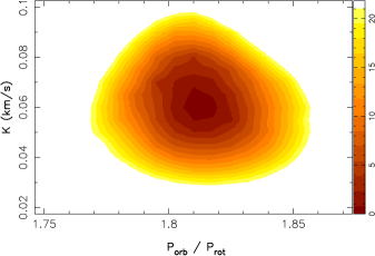
Figure 10: Variations of $\Delta\chi^{2}$ of the ZDI fits to the late-2015 and early-2016 LSD profiles of V830 Tau (for a fixed spottedness level at both epochs), after removing the reflex motion of a close-in a planet and for a range of orbital periods $P_{\rm orb}$ (actually the ratio of the orbital to rotation period $\hbox{$P_{\rm orb}$}/\hbox{$P_{\rm rot}$}$) and semi-amplitudes $K$ of the planet RV signature. (This is a 2D cut from a 3D map, with the phase of the RV signal also included as a search parameter). A clear minimum is obtained in the $\Delta\chi^{2}$ landscape, whose projection in a $K$ vs $\hbox{$P_{\rm orb}$}/\hbox{$P_{\rm rot}$}$ plane passing through the minimum is shown here. The outer color contour traces the projected 99.99% confidence interval, corresponding to a $\Delta\chi^{2}$ of 21.1 for a 3-parameter fit to the 3312 data points of the LSD profiles.

4.3 Deriving planet parameters from raw RVs using Gaussian-process regression (GPR)

The third method we applied to our data works directly from raw RVs and uses GPR to model the activity jitter as well as its temporal evolution, given its covariance function (e.g., Haywood et al., 2014; Rajpaul et al., 2015). Assuming again the presence of a close-in planet of given characteristics, we correct the raw RVs from the reflex motion induced by the planet and fit the corrected RVs with a Gaussian process (GP) based on a pseudo-periodic covariance function $c(t,t^{\prime})$ of the form:

$$c(t,t^{\prime}) = \theta_{1}^{2}\exp\left(-\frac{(t-t^{\prime})^{2}}{\theta_{3}^{2}}-\frac{\sin^{2}\left(\frac{\pi(t-t^{\prime})}{\theta_{2}}\right)}{\theta_{4}^{2}}\right)$$ (3)

where $\theta_{1}$ is the amplitude of the GP (in km s^-1), $\theta_{2}$ the recurrence timescale (i.e., close to 1 here, in units of $P_{\rm rot}$), $\theta_{3}$ the decay timescale (i.e., the typical spot lifetime here, in units of $P_{\rm rot}$) and $\theta_{4}$ a smoothing parameter (within [0,1]) setting the amount of high frequency structure that we allow the fit to include. For a given set of planet parameters and of the 4 GP hyper parameters $\theta_{1}$ to $\theta_{4}$, we can compute the GP that best fits the corrected raw RVs (denoted $y$) and estimate the log likelihood $\log\mathcal{L}$ of the corresponding parameter set from:

$$2\log\mathcal{L} = -n\log(2\pi)-\log|C+\Sigma|-y^{T}(C+\Sigma)^{-1}y$$ (4)

where $C$ is the covariance matrix for all observing epochs, $\Sigma$ the diagonal variance matrix of the raw RVs and $n$ the number of data points. Coupling this with a Markov Chain Monte-Carlo (MCMC) simulation to explore the parameter domain, we can determine the optimal set of planet and GP hyper parameters that maximizes likelihood, as well as the relative probability of this optimal model with respect to one with no planet (and only the GP modelling activity).

We start by carrying out an initial MCMC run with input priors, whose results (the posterior distributions) are used to infer refined priors and proposal distributions capable of ensuring both an efficient mixing and convergence of the chain as well as a thorough exploration of the domain of interest (through a standard Metropolis-Hastings jumping scheme); these refined priors are found to be weakly dependent on the input priors, already suggesting that our data contain enough information to reliably characterize the GP and planet parameters. The main MCMC run uses our refined priors, listed in Table 4 for the various parameters; we usually carry out two successive main runs, a first one with all 4 GP hyper parameters and 3 planet parameters free to vary, then a second one with both $\theta_{3}$ and $\theta_{4}$ fixed to their best values and the remaining 5 parameters left free to vary. The goal of this sequential approach is to incorporate as much prior information about the stellar activity as possible into our model (hence the stronger refined priors) so that the GP yields a robust estimation of the uncertainties on the final parameters (particularly the planet mass) given these priors (see Haywood et al. 2014 and Lopez-Morales et al. 2016 for a similar approach).

Table 4: Priors used in our MCMC simulation for the planet and GP hyper parameters. We mention the mean and standard deviation used for the refined Gaussian priors (plus the standard deviation assumed for our initial MCMC run), the minimum and maximum values allowed for the uniform and Jeffreys priors, as well as the knee value for the modified Jeffreys priors (following Haywood et al. 2014, with $\sigma_{\rm RV}$ noting the $\hbox{S/N}^{2}$-weighted average RV error of our measurements, equal to 53 m s^-1, see Table 1). The planet phase $\phi_{0}$ relates to the epoch of inferior conjunction BJD_t through $\hbox{BJD${}_{\rm t}$}=\phi_{0}\hbox{$P_{\rm orb}$}+t_{0}$ where $t_{0}=2,457,359.9069$ d (corresponding to rotation cycle 127.0) is the reference zero time we used for our observations.

Parameter	Prior
$P_{\rm orb}$/$P_{\rm rot}$	Gaussian (1.80, 0.012, initial 0.10)
$K$ (km s-1)	modified Jeffreys ($\sigma_{\rm RV}$)
$\phi_{0}$	Gaussian (0.13, 0.04, initial 0.10)
GP amplitude $\theta_{1}$ (km s-1)	modified Jeffreys ($\sigma_{\rm RV}$)
Recurrence period $\theta_{2}$ ($P_{\rm rot}$)	Gaussian (1.0, 0.001, initial 0.010)
Spot lifetime $\theta_{3}$ ($P_{\rm rot}$)	Jeffreys (0.1, 500.0)
Smoothing parameter $\theta_{4}$	Uniform (0, 1)

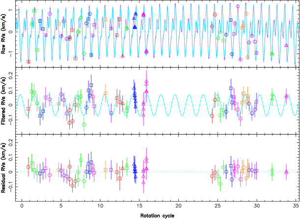
Figure 11: Same as Fig. 8 but now using a planet+GP fit to the data (pink line), where the GP is modelling the activity jitter (cyan line) while the planet and GP parameters are determined using a MCMC simulation. Note how the GP succeeds at modelling the activity and its temporal evolution throughout the whole observing window, and not just for the two separate subsets. The rms dispersion of the residual RVs is 37 m s^-1.

We find that $\theta_{3}$, the hyper parameter describing spot lifetime, gives the best result for a value of $\theta_{3}=44\pm 11~{}\hbox{$P_{\rm rot}$}=120\pm 30$ d, only slightly longer than the full duration of our observing run (91 d). This further confirms the importance of taking into account the temporal evolution of brightness maps in activity filtering studies, even in the case of wTTSs like V830 Tau whose spot distributions are known to be fairly stable on long timescales; whereas this is true for the largest surface features, this is no longer the case for the smaller ones whose effect on RV curves is significant. Similarly, we get that $\theta_{4}=0.6\pm 0.1$ yields the most likely fit to the data; this reflects the lack of fine structure in the RV curves, as expected from the fact that RVs are the first-order moment of Stokes $I$ LSD profiles that acts as a low-pass filter on surface brightness distributions. With the final MCMC run, we obtain that the recurrence timescale $\theta_{2}$ is equal to $\theta_{2}=0.9986\pm 0.0007~{}\hbox{$P_{\rm rot}$}$, i.e., only very slightly shorter than the average rotation period $P_{\rm rot}$ on which our data were phased (see Eq. 2); we note that this period matches well the equatorial rotation period of V830 Tau (see Table 3 and Sec. 3.2), suggesting that RVs are primarily affected by equatorial features at the stellar surface. For the GP amplitude $\theta_{1}$, we find that $\theta_{1}=0.878\pm 0.135$ km s^-1, $\simeq$30% larger than the rms dispersion of our raw RVs (equal to 0.65 km s^-1 prior to any activity filtering, or removal of planetary-induced reflex motions).

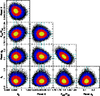
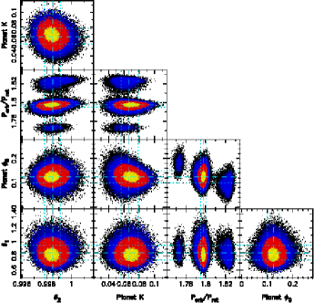
Figure 14: Phase plots of our final 5-parameter MCMC run using both the late 2015 and early 2016 data (left) and all raw RVs collected to date on V830 Tau (right), with yellow, red and blue points marking the 1, 2 and 3-$\sigma$ confidence regions respectively. The optimal parameter we derive from the left panel are respectively equal to $\theta_{1}=0.878\pm 0.135$ km s^-1, $\theta_{2}=0.9986\pm 0.0007~{}\hbox{$P_{\rm rot}$}$, $K=68\pm 11$ m s^-1, $\hbox{$P_{\rm orb}$}/\hbox{$P_{\rm rot}$}=1.80\pm 0.01$ (i.e., $\hbox{$P_{\rm orb}$}=4.93\pm 0.03$ d) and $\phi_{0}=0.122\pm 0.028$ (i.e., $\hbox{BJD${}_{\rm t}$}=2,457,360.51\pm 0.14$ d). Fitting all raw RVs allows to significantly improve the precision on the rotation period ($\hbox{$P_{\rm orb}$}/\hbox{$P_{\rm rot}$}=1.7976\pm 0.0027\pm 0.01$, i.e., $\hbox{$P_{\rm orb}$}=4.927\pm 0.008$ d) and to slightly refine the epoch of inferior conjunction ($\phi_{0}=0.125\pm 0.025$, i.e., $\hbox{BJD${}_{\rm t}$}=2,457,360.523\pm 0.124$ d). Note the little correlation between the various parameters.

For the planet parameters, we find that $K=68\pm 11$ m s^-1 and $\hbox{$P_{\rm orb}$}=4.93\pm 0.03$ d, whereas the most accurate epoch of inferior conjunction (assuming a circular orbit) is found to be $\hbox{BJD${}_{\rm t}$}=2,457,360.51\pm 0.14$. The corresponding fit to the data, shown in Fig. 11, demonstrates that the GP is doing a very nice job at modelling not only the activity, but also its evolution with time. Comparing with the results of our first method (see Fig. 8), we can see that both the GP and ZDI predict similar RV curves. However, thanks to its higher flexibility, the GP does a better job at matching the data, not only for our second data set where temporal variability is higher (given the faster evolution of the predicted RV curve, see Fig. 11) and where the planet signal is clearly better recovered, but also for our first data set where the slower spot evolution is enhanced by the longer time span (of 15 rotation cycles). As a result, the rms dispersion of the RV residuals has further decreased to 37 m s^-1, 16% smaller than with our first method, including in the first part of our run (late 2015) where the fit to the data is now tighter (rms dispersion of RV residuals of 40 m s^-1 instead of 50 m s^-1, and close to that of the full run). Given this, we consider that the planet parameters derived with this third method, and in particular $K$ and $P_{\rm orb}$, are likely more accurate than the estimates obtained with the two previous techniques; they also agree better with the initial estimates of D16 inferred from the late 2015 data only. The phase plots of our final 5-parameter MCMC run are provided in Appendix A (see Fig. 14, left panel), showing little correlation between the various parameters and thus minimum bias in the derived values.

When applying this technique to the full series of raw RVs collected to date on V830 Tau, including our original set secured in late 2014 and early 2015 (D15, D16), we further enhance the precision on the derived parameters, in particular on the orbital period that we can now pin down to $\hbox{$P_{\rm orb}$}=4.927\pm 0.008$ d. The derived semi-amplitude of the RV curve is the same as in the previous fit ($K=68\pm 11$ m s^-1) whereas the epoch of inferior conjunction (assuming a circular orbit) is only slightly improved ($\hbox{BJD${}_{\rm t}$}=2,457,360.522\pm 0.124$). The phase plots of this MCMC run are also provided in Appendix A (see Fig. 14, right panel).

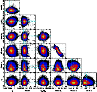
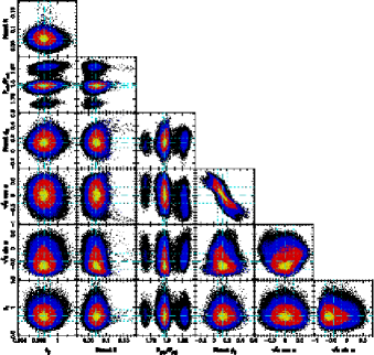
Figure 15: Same as Fig. 14 when fitting an eccentric orbit using parameter $\sqrt{e}\cos\omega$ and $\sqrt{e}\sin\omega$ as search parameters where $e$ and $\omega$ respectively denote the eccentricity and argument of periapsis of the orbit; the marginal likelihood of the best eccentric orbit model is not significantly larger than that of the best circular orbit model, implying that there is no evidence that the planet is eccentric.

Applying the method of Chib & Jeliazkov (2001) to the MCMC posterior samples, we obtain that the marginal likelihood of the model including the planet is higher than that of a model with no planet by a Bayes’ factor of $10^{8}$ ($10^{9}$ when also including our raw RVs from late 2014 and early 2015), providing a strong and independent confirmation that V830 Tau hosts a close-in giant planet in a 4.93 d orbit. Assuming now a planet on an elliptical orbit (and using $\sqrt{e}\cos\omega$ and $\sqrt{e}\sin\omega$ as search parameters where $e$ and $\omega$ respectively denote the eccentricity and argument of periapsis of the orbit, Ford 2006) yields a low eccentricity of $0.16\pm 0.20$; the marginal likelihood of this latter model is however larger than that of the circular planet model by a Bayes’ factor of $<3$, implying that there is no evidence yet that the planet is eccentric. We provide the MCMC phase plots of the eccentric orbit model in Fig. 15.

The planet parameters derived with all 3 methods are summarized in Table 5, with those derived in D16 (from our late 2015 data only) listed as well for an easy comparison.

Table 5: Summary of our results using the three filtering techniques described in Sec. 4; columns 2 to 4 are for the 2 ZDI-based and GPR methods described in Secs. 4.1 to 4.3 and applied to our new data from late 2015 to early 2016, whereas column 5 is for GPR applied to the entire data set (including that of D15). Column 6 recalls the results derived in D16 from the late 2015 data only as a comparison. The first table section lists the derived planet parameters (with $M_{\rm p}$ denoting the planet mass), the second one mentions the inferred GP hyper parameters in the GPR case, and the last one recalls the achieved $\chi^{2}_{\rm r}$ (to the filtered RVs for ZDI #1, to the Stokes $I$ profiles for ZDI #2 and to the raw RVs for GPR) and the rms dispersion of the RV residuals (whenever relevant).

Parameter	ZDI #1	ZDI #2	GPR	GPR (all data)	D16
$P_{\rm orb}$ (d)	$4.97\pm 0.03$	$4.97\pm 0.03$	$4.93\pm 0.03$	$4.927\pm 0.008$	$4.93\pm 0.05$
$K$ (m s-1)	$60\pm 10$	$62\pm 9$	$68\pm 11$	$68\pm 11$	$75\pm 12$
$\phi_{0}$	$0.128\pm 0.025$	$0.142\pm 0.024$	$0.122\pm 0.028$	$0.125\pm 0.025$	$0.123\pm 0.025$
BJDt (2,457,300+)	$60.54\pm 0.13$	$60.61\pm 0.12$	$60.51\pm 0.14$	$60.523\pm 0.124$	$60.52\pm 0.13$
$M_{\rm p}\sin i$ (${\rm M}_{\rm Jup}$)	$0.50\pm 0.09$	$0.52\pm 0.09$	$0.57\pm 0.10$	$0.57\pm 0.10$	$0.63\pm 0.10$
$M_{\rm p}$ (${\rm M}_{\rm Jup}$) assuming $i=55\hbox{${}^{\circ}$}$	$0.61\pm 0.11$	$0.63\pm 0.11$	$0.70\pm 0.12$	$0.70\pm 0.12$	$0.77\pm 0.12$
$a$ (au)				$0.057\pm 0.001$
$a/\hbox{$R_{\star}$}$				$6.1\pm 0.6$
GP amplitude $\theta_{1}$ (km s-1)			$0.878\pm 0.135$	$0.842\pm 0.105$
Recurrence period $\theta_{2}$ ($P_{\rm rot}$)			$0.9986\pm 0.0007$	$0.9985\pm 0.0006$
Spot lifetime $\theta_{3}$ (d)			$120\pm 30$
Smoothing parameter $\theta_{4}$			$0.6\pm 0.1$
$\chi^{2}_{\rm r}$	0.68	1.0	0.48	0.42	0.75
rms RV residuals (m s-1)	44		37	35	48

5 Summary & discussion

This paper reports the results of an extended spectropolarimetric run on the wTTS V830 Tau, carried out in the framework of the international MaTYSSE Large Programme, using ESPaDOnS on the CFHT, Narval on the TBL and GRACES/ESPaDOnS on Gemini-North, spanning from 2015 Nov 11 to Dec 22, then from 2016 Jan 14 to Feb 10, and complemented by contemporaneous photometric observations from the 1.25-m telescope at CrAO. This new study is an in-depth follow-up of a previous one, based only on the first part of this data set and focussed on the detection of the young close-in hJ orbiting V830 Tau in 4.93 d (D16), and of an older one that suspected the presence of V830 Tau b, but from too sparse a data set to firmly demonstrate the existence of the planet (D15).

Applying ZDI to our two new data subsets, we derived the surface brightness and magnetic maps of V830 Tau. Cool spots and warm plages are again present on V830 Tau, totalling 13% of the overall stellar surface for those to which ZDI is sensitive. The brightness maps from late 2015 and early 2016 are similar, except for differential rotation slightly shearing the photosphere of V830 Tau and for small local changes in the spot distribution, reflecting their temporal evolution on a timescale of only a few weeks. The magnetic maps of V830 Tau are also quite similar at both epochs and to that reconstructed from our previous data set (D15), featuring a mainly poloidal field whose dominant component is a 340 G dipole tilted at 22^∘ from the rotation axis. As for the brightness distribution, the magnetic field is also sheared by a weak surface differential rotation, and is evolving with time over the duration of our observing run.

We detected several flares of V830 Tau during the second part of our run, where one major event and a weaker precursor were strong enough to impact RVs at a level of about 0.3 km s^-1. In addition to generate intense emission in the usual spectral activity proxies including the H${\alpha}$, Ca ii IRT and He i $D_{3}$ lines, these flares triggered large redshifts of the emission component, especially for the He i $D_{3}$ line whose redshift reaches up to 35 km s^-1 with respect to the stellar rest frame, and 25 km s^-1 with respect to the average line position in a quiet state. By analogy with the Sun and young active stars (e.g., Collier Cameron & Robinson, 1989a, b), we propose that the flares we detect on V830 Tau relate to coronal mass ejections and reflect the presence of massive prominences in the magnetosphere of V830 Tau, likely confined by magnetic fields in the equatorial belt of closed-field loops encircling the star (see Fig. 6), and whose stability is perturbed by the photospheric shear stressing the field or by the hot Jupiter itself in the case of large magnetic loops extending as far as the giant planet orbit (at 6.1 $R_{\star}$). High-cadence spectral monitoring in various activity proxies is required to investigate such flares in more detail, work out the fate of associated prominences once no longer magnetically confined, and diagnose the main triggering mechanism behind them.

We applied 3 different methods to our full data set to further confirm the existence of its hJ, and better characterize its orbital parameters. The first two methods, using ZDI to model and predict the RV activity jitter, are those with which V830 Tau b was originally detected, in a slightly modified version allowing them to handle two different ZDI images (corresponding to the late-2015 and early-2016 subsets) at the same time and account for the potential evolution of brightness distributions between the 2 epochs. Our third technique is fully independent from the 2 others and directly works from raw RVs, using GPR to model the RV activity jitter and MCMC to infer the optimal planet and GP parameters and error bars in a Bayesian formalism, following Haywood et al. (2014). All 3 methods unambiguously confirm the existence of V830 Tau b and yield consistent results for the planet parameters when applied to our new data; in particular, all are able to reliably recover the RV planet signal (of semi-amplitude $68\pm 11$ m s^-1) hiding behind the activity jitter (of semi-amplitude 1.2 km s^-1 and rms dispersion 0.65 km s^-1) that the brightness distribution of V830 Tau is inducing. The third method is found to perform best, thanks to its higher flexibility and better performances at modelling the temporal evolution of the RV activity jitter. Applying this third method to all raw RVs collected to date on V830 Tau (including those of D15) allows us to significantly improve the precision on the planet orbital period. We also confirm that the planet orbit is more or less circular, with no evidence for a non-zero eccentricity at a 1$\sigma$ precision of 0.15–0.20. Further work is needed to enable ZDI reconstructing time-variable features and make it as efficient as GPR for filtering activity from RV curves of young active stars.

Spectropolarimetry is found to be essential for retrieving the large-scale topology of the magnetic field that fuels all activity phenomena, but not critical for modelling and filtering the activity jitter at optical wavelengths, largely dominated by the impact of surface brightness features; however, spectropolarimetry is expected to become crucial at nIR wavelengths where brightness features contribute less jitter and Zeeman distortions are much larger than in the optical (e.g., Reiners et al., 2013; Hébrard et al., 2014).

Along with the latest reports of similar detections (or candidate detections) of young close-in giants around TTSs (e.g., van Eyken et al., 2012; Mann et al., 2016; Johns-Krull et al., 2016; David et al., 2016; Yu et al., 2016), our result suggests that newborn hJs may be frequent, possibly more so than their mature equivalents around Sun-like stars (Wright et al., 2012). The orbital fate of young hJs like V830 Tau b under tidal forces and strong winds as the host star progresses on its evolutionary track, contracts and spins up to the main sequence, and at the same time loses angular momentum to its magnetic wind and planet, is still unclear (e.g., Vidotto et al., 2010; Bolmont & Mathis, 2016). One can expect V830 Tau b, whose orbital period is currently longer than the stellar spin period, to be spiralling outwards, at least until V830 Tau is old enough to rotate more slowly than its close-in giant; investigating whether tidal forces will still be strong enough by then to successfully drag V830 Tau b back and kick it into its host star in the next few hundred Myrs, may tell whether and how frequent newborn close-in giants can be reconciled with the observed sparse population of mature hJs.

Alternatively, the MaTYSSE sample may be somehow biased towards wTTSs hosting hJs (e.g., Yu et al., 2016). In particular, our sample is likely biased towards wTTSs whose discs have dissipated early, i.e., at a time where the star, still fully convective, hosted a magnetic field strong enough to carve a large magnetospheric gap (Gregory et al., 2012; Donati et al., 2013) and trigger stable accretion (Blinova et al., 2016). This may come as favorable conditions for hJs to survive type-II migration, when compared to more evolved cTTSs featuring weaker fields, smaller magnetospheric gaps and chaotic accretion.

Last but not least, we stress that V830 Tau is the first known non-solar planet host that exhibits radio emission (Bower et al., 2016), which opens very exciting perspectives for in-depth studies of star-planet interactions, and possibly even of exoplanetary magnetic fields (Vidotto et al., 2010; Vidotto & Donati, 2016).

Applying the complementary detection techniques outlined in this paper to extended spectropolarimetric data sets such as those gathered within MaTYSSE, or forthcoming ones to be collected with SPIRou, the nIR spectropolarimeter / high-precision velocimeter currently in construction for CFHT (first light planned in 2017), should turn out extremely fruitful and enlightening for our understanding of star / planet formation, about which little observational constraints yet exist.

Appendix A Additional figures

   

                   

   

   

¹Université de Toulouse, UPS-OMP, IRAP, 14 avenue E. Belin, Toulouse, F–31400 France
²CNRS, IRAP / UMR 5277, Toulouse, 14 avenue E. Belin, F–31400 France
³CFHT Corporation, 65-1238 Mamalahoa Hwy, Kamuela, Hawaii 96743, USA
⁴SUPA, School of Physics and Astronomy, Univ. of St Andrews, St Andrews, Scotland KY16 9SS, UK
⁵Département de physique, Université de Montréal, C.P. 6128, Succursale Centre-Ville, Montréal, QC, Canada H3C 3J7
⁶Crimean Astrophysical Observatory, Nauchny, Crimea 298409
⁷Department of Physics and Astronomy, York University, Toronto, Ontario L3T 3R1, Canada
⁸ESO, Karl-Schwarzschild-Str. 2, D-85748 Garching, Germany
⁹School of Physics, Trinity College Dublin, the University of Dublin, Ireland
¹⁰Departamento de Fìsica – ICEx – UFMG, Av. Antônio Carlos, 6627, 30270-901 Belo Horizonte, MG, Brazil
¹¹Harvard-Smithsonian Center for Astrophysics, 60 Garden Street, Cambridge, MA 02138, USA
¹²Université Grenoble Alpes, IPAG, BP 53, F–38041 Grenoble Cédex 09, France
¹³CNRS, IPAG / UMR 5274, BP 53, F–38041 Grenoble Cédex 09, France
¹⁴Institute of Astronomy and Astrophysics, Academia Sinica, PO Box 23-141, 106, Taipei, Taiwan
¹⁵Kavli Institute for Astronomy and Astrophysics, Peking University, Yi He Yuan Lu 5, Haidian Qu, Beijing 100871, China
¹⁶LUPM, Université de Montpellier, CNRS, place E. Bataillon, F–34095 Montpellier, France

References

- Aigrain et al. (2012) Aigrain S., Pont F., Zucker S., 2012, MNRAS, 419, 3147
- André et al. (2009) André P., Basu S., Inutsuka S., 2009, The formation and evolution of prestellar cores. Cambridge University Press, p. 254
- Baruteau et al. (2014) Baruteau C., et al., 2014, Protostars and Planets VI, pp 667–689
- Blinova et al. (2016) Blinova A. A., Romanova M. M., Lovelace R. V. E., 2016, MNRAS, 459, 2354
- Bolmont & Mathis (2016) Bolmont E., Mathis S., 2016, Celestial Mechanics and Dynamical Astronomy,
- Bouvier et al. (2007) Bouvier J., Alencar S. H. P., Harries T. J., Johns-Krull C. M., Romanova M. M., 2007, in Reipurth B., Jewitt D., Keil K., eds, Protostars and Planets V. pp 479–494
- Bower et al. (2016) Bower G. C., Loinard L., Dzib S., Galli P. A. B., Ortiz-León G. N., Moutou C., Donati J.-F., 2016, ApJ, 830, 107
- Brown et al. (1991) Brown S. F., Donati J.-F., Rees D. E., Semel M., 1991, A&A, 250, 463
- Chene et al. (2014) Chene A.-N., et al., 2014, in Advances in Optical and Mechanical Technologies for Telescopes and Instrumentation. p. 915147 (arXiv:1409.7448), doi:10.1117/12.2057417
- Chib & Jeliazkov (2001) Chib S., Jeliazkov I., 2001, Journal of the American Statistical Association, 96, 270
- Collier Cameron & Robinson (1989a) Collier Cameron A., Robinson R. D., 1989a, MNRAS, 236, 57
- Collier Cameron & Robinson (1989b) Collier Cameron A., Robinson R. D., 1989b, MNRAS, 238, 657
- David et al. (2016) David T. J., et al., 2016, Nature, 534, 658
- Donati (2001) Donati J.-F., 2001, in Boffin H. M. J., Steeghs D., Cuypers J., eds, Lecture Notes in Physics, Berlin Springer Verlag Vol. 573, Astrotomography, Indirect Imaging Methods in Observational Astronomy. p. 207
- Donati (2003) Donati J.-F., 2003, in Trujillo-Bueno J., Sanchez Almeida J., eds, Astronomical Society of the Pacific Conference Series Vol. 307, Astronomical Society of the Pacific Conference Series. p. 41
- Donati & Brown (1997) Donati J.-F., Brown S. F., 1997, A&A, 326, 1135
- Donati & Collier Cameron (1997) Donati J.-F., Collier Cameron A., 1997, MNRAS, 291, 1
- Donati et al. (1997) Donati J.-F., Semel M., Carter B. D., Rees D. E., Collier Cameron A., 1997, MNRAS, 291, 658
- Donati et al. (2003) Donati J.-F., Collier Cameron A., Petit P., 2003, MNRAS, 345, 1187
- Donati et al. (2006) Donati J.-F., et al., 2006, MNRAS, 370, 629
- Donati et al. (2007) Donati J.-F., et al., 2007, MNRAS, 380, 1297
- Donati et al. (2008) Donati J.-F., et al., 2008, MNRAS, 385, 1179
- Donati et al. (2010) Donati J., et al., 2010, MNRAS, 409, 1347
- Donati et al. (2011) Donati J., et al., 2011, MNRAS, 412, 2454
- Donati et al. (2012) Donati J.-F., et al., 2012, MNRAS, 425, 2948
- Donati et al. (2013) Donati J.-F., et al., 2013, MNRAS, 436, 881
- Donati et al. (2014) Donati J.-F., et al., 2014, MNRAS, 444, 3220
- Donati et al. (2015) Donati J.-F., et al., 2015, MNRAS, 453, 3706
- Donati et al. (2016) Donati J. F., et al., 2016, Nature, 534, 662
- Ford (2006) Ford E. B., 2006, ApJ, 642, 505
- Frank et al. (2014) Frank A., et al., 2014, Protostars and Planets VI, pp 451–474
- Grankin (2013) Grankin K. N., 2013, Astronomy Letters, 39, 251
- Grankin et al. (2008) Grankin K. N., Bouvier J., Herbst W., Melnikov S. Y., 2008, A&A, 479, 827
- Gregory et al. (2012) Gregory S. G., Donati J.-F., Morin J., Hussain G. A. J., Mayne N. J., Hillenbrand L. A., Jardine M., 2012, ApJ, 755, 97
- Haywood et al. (2014) Haywood R. D., et al., 2014, MNRAS, 443, 2517
- Haywood et al. (2016) Haywood R. D., et al., 2016, MNRAS, 457, 3637
- Hébrard et al. (2014) Hébrard É. M., Donati J.-F., Delfosse X., Morin J., Boisse I., Moutou C., Hébrard G., 2014, MNRAS, 443, 2599
- Hussain et al. (2009) Hussain G. A. J., et al., 2009, MNRAS, 398, 189
- Jardine (2004) Jardine M., 2004, A&A, 414, L5
- Johns-Krull (2007) Johns-Krull C. M., 2007, ApJ, 664, 975
- Johns-Krull et al. (1999) Johns-Krull C. M., Valenti J. A., Koresko C., 1999, ApJ, 516, 900
- Johns-Krull et al. (2016) Johns-Krull C. M., et al., 2016, ApJ, 826, 206
- Landi degl’Innocenti & Landolfi (2004) Landi degl’Innocenti E., Landolfi M., 2004, Polarisation in spectral lines. Dordrecht/Boston/London: Kluwer Academic Publishers
- Lin et al. (1996) Lin D. N. C., Bodenheimer P., Richardson D. C., 1996, Nature, 380, 606
- Lopez-Morales et al. (2016) Lopez-Morales M., et al., 2016, preprint, (arXiv:1609.07617)
- Lucy & Sweeney (1971) Lucy L. B., Sweeney M. A., 1971, AJ, 76, 544
- Mann et al. (2016) Mann A. W., et al., 2016, AJ, 152, 61
- Montes et al. (1997) Montes D., Fernandez-Figueroa M. J., de Castro E., Sanz-Forcada J., 1997, A&AS, 125
- Morin et al. (2008) Morin J., et al., 2008, MNRAS, 390, 567
- Moutou et al. (2007) Moutou C., et al., 2007, A&A, 473, 651
- Petit et al. (2015) Petit P., et al., 2015, A&A, 584, A84
- Rajpaul et al. (2015) Rajpaul V., Aigrain S., Osborne M. A., Reece S., Roberts S., 2015, MNRAS, 452, 2269
- Reiners et al. (2013) Reiners A., Shulyak D., Anglada-Escudé G., Jeffers S. V., Morin J., Zechmeister M., Kochukhov O., Piskunov N., 2013, A&A, 552, A103
- Rodríguez et al. (2012) Rodríguez L. F., González R. F., Raga A. C., Cantó J., Riera A., Loinard L., Dzib S. A., Zapata L. A., 2012, A&A, 537, A123
- Romanova & Lovelace (2006) Romanova M. M., Lovelace R. V. E., 2006, ApJ, 645, L73
- Siess et al. (2000) Siess L., Dufour E., Forestini M., 2000, A&A, 358, 593
- Vidotto & Donati (2016) Vidotto A. A., Donati J.-F., 2016, A&A, p. submitted
- Vidotto et al. (2010) Vidotto A. A., Opher M., Jatenco-Pereira V., Gombosi T. I., 2010, ApJ, 720, 1262
- Wright et al. (2012) Wright J. T., Marcy G. W., Howard A. W., Johnson J. A., Morton T. D., Fischer D. A., 2012, ApJ, 753, 160
- Yu et al. (2016) Yu L., Donati J.-F., Hébrard E., Moutou S., et al., 2016, MNRAS, p. submitted
- van Eyken et al. (2012) van Eyken J. C., et al., 2012, ApJ, 755, 42