Linear Convergence of SVRG　 in Statistical Estimation

Abstract

The last several years has witness the huge success on the stochastic variance reduction method in the finite sum problem. However assumption on strong convexity to have linear rate limits its applicability. In particular, it does not include several important formulations such as Lasso, group Lasso, logistic regression, and some non-convex models including corrected Lasso and SCAD. In this paper, we prove that, for a class of statistical M-estimators covering examples mentioned above, SVRG solves the formulation with a linear convergence rate without strong convexity or even convexity. Our analysis makes use of restricted strong convexity, under which we show that SVRG converges linearly to the fundamental statistical precision of the model, i.e., the difference between true unknown parameter $\theta^{*}$ and the optimal solution $\hat{\theta}$ of the model.

1 Introduction

In this paper we establish fast convergence rate of stochastic variance reduction gradient (SVRG) for a class of problems motivated by applications in high dimensional statistics where the problems are not strongly convex, or even non-convex. High-dimensional statistics has achieved remarkable success in the last decade, including results on consistency and rates for various estimator under non-asymptotic high-dimensional scaling, especially when the problem dimension $p$ is larger than the number of data $n$ (e.g., Negahban et al., 2009; Candès and Recht, 2009, and many others (Candes et al., 2006; Wainwright, 2006; Chen et al., 2011)) . It is now well known that while this setup appears ill-posed, the estimation or recovery is indeed possible by exploiting the underlying structure of the parameter space – notable examples include sparse vectors, low-rank matrices, and structured regression functions, among others. Recently, estimators leading to non-convex optimizations have gained fast growing attention. Not only it typically has better statistical properties in the high dimensional regime, but also in contrast to common belief, under many cases there exist efficient algorithms that provably find near-optimal solutions Loh and Wainwright (2011); Zhang and Zhang (2012); Loh and Wainwright (2013) .

Computation challenges of statistical estimators and machine learning algorithms have been an active area of study, thanks to countless applications involving big data – datasets where both $p$ and $n$ are large. In particular, there are renewed interests in first order methods to solves the following class of optimization problems:

$$\begin{split}\underset{\theta\in\Omega}{\mbox{Minimize:}}\quad G(\theta)&\triangleq F(\theta)+\lambda\psi(\theta)\\ &=\frac{1}{n}\sum_{i=1}^{n}f_{i}(\theta)+\lambda\psi(\theta).\end{split}$$ (1)

Problem (1) naturally arises in statistics and machine learning. In supervised learning, we are given a sample of $n$ training data $(x_{1},y_{1}),(x_{2},y_{2}),...,(x_{n},y_{n})$, and thus $f_{i}(\theta)$ is the corresponding loss, e.g., the squared loss $f_{i}(\theta)=(y_{i}-\theta^{T}x_{i})^{2}$, $\Omega$ is a convex set corresponding to the class of hypothesis, and $\psi(\theta)$ is the (possibly non-convex) regularization. Many widely applied statistical formulations are examples of Problem (1). A partial list includes:

• Lasso: $f_{i}(\theta)=\frac{1}{2}(\langle\theta,x_{i}\rangle-y_{i})^{2}$ and $\psi(\theta)=\|\theta\|_{1}$.

• Group Lasso: $f_{i}(\theta)=\frac{1}{2}(\langle\theta,x_{i}\rangle-y_{i})^{2}$, $\psi(\theta)=\|\theta\|_{1,2}$.

• Logistic Regression with $l_{1}$ regularization: $f_{i}(\theta)=\log(1+\exp(-y_{i}\langle x_{i},\theta\rangle)$ and $\psi(\theta)=\|\theta\|_{1}$.

• Corrected Lasso Loh and Wainwright (2011): $G(\theta)=\sum_{i=1}^{n}\frac{1}{2n}(\langle\theta,x_{i}\rangle-y_{i})^{2}-\frac{1}{2}\theta^{T}\Sigma\theta+\lambda\|\theta\|_{1},$ where $\Sigma$ is some positive definite matrix.

• Regression with SCAD regularizer Fan and Li (2001): $G(\theta)=\sum_{i=1}^{n}\frac{1}{2n}(\langle\theta,x_{i}\rangle-y_{i})^{2}+SCAD(\theta)$.

In the first three examples, the objective functions $G(\theta)$ are not strongly convex when $p>n$. Example 4 is non-convex when $p>n$, and the last example is non-convex due to the SCAD regularizer.

Projected gradient method, proximal gradient method, dual averaging method Nesterov (2009) and several variants of them have been proposed to solve Problem (1). However, at each step, these batched gradient descent methods need to evaluate all $n$ derivatives, corresponding to each $f_{i}(\cdot)$, which can be expensive for large $n$. Accordingly, stochastic gradient descent (SGD) methods have gained attention, because of its significantly lighter computation load for each iteration: at iteration $t$, only one data point – sampled from $\{1,...,n\}$ and indexed by $i_{t}$ – is used to update the parameter $\theta$ according to

$$\theta_{t+1}:=\theta_{t}-\beta\nabla f_{i_{t}}(\theta_{t}),$$

or its proximal counterpart (w.r.t. the regularization function $\psi(\cdot)$)

$$\theta_{t+1}:=Prox_{\beta\lambda\psi}(\theta_{t}-\beta\nabla f_{i_{t}}(\theta_{t})).$$

Although the computational cost in each step is low, SGD often suffers from slow convergence, i.e., sub-linear convergence rate even with strong assumptions (strong convexity and smoothness). Recently, one state-of-art technique to improve the convergence of SGD called the variance-reduction-gradient has been proposed Johnson and Zhang (2013); Xiao and Zhang (2014). As the name suggests, it devises a better unbiased estimator of stochastic gradient $v_{t}$ such that the variance $E\|v_{t}-\nabla F(\theta_{t})\|_{2}$ diminishes when $t\rightarrow\infty$. In particular, in SVRG and its variants, the algorithm keeps a snapshot $\tilde{\theta}$ after every $m$ SGD iterations and calculate the full gradient $F(\tilde{\theta})$ just for this snapshot, then the variance reduced gradient is computed by

$$v_{t}=\nabla f_{i_{t}}(\theta_{t})-\nabla f_{i_{t}}(\tilde{\theta})+\nabla F(\tilde{\theta}).$$

It is shown in Johnson and Zhang (2013) that when $G(\theta)$ is strongly convex and $F(\theta)$ is smooth, SVRG and its variants enjoy linear convergence, i.e., $O(\log(1/\epsilon))$ steps suffices to obtain an $\epsilon$-optimal solution. Equivalently, the gradient complexity (i.e., the number of gradient evaluation needed) is $O((n+\frac{L}{\mu})\log(1/\epsilon))$, where $L$ is the smoothness of $F(\theta)$ and $\mu$ is the strong convexity of $F(\theta)$.

What if $G$ is not strongly convex or even not convex? As we discussed above, many popular machine learning models belongs to this. When $G$ is not strongly convex, existing theory only guarantees that SVRG will converge sub-linearly. A folklore method is to add a dummy strongly convex term $\frac{\sigma}{2}\|\theta\|_{2}^{2}$ to the objective function and then apply the algorithm Shalev-Shwartz and Zhang (2014); Allen-Zhu and Yuan (2015). This undermines the performance of the model, particularly its ability to recover sparse solutions. One may attempt to reduce $\sigma$ to zero in the hope of reproducing the optimal solution of the original formulation, but the convergence will still be sub-linear via this approach. As for the non-convex case , to the best of our knowledge, no work provides linear convergence guarantees for the above mentioned examples using SVRG.

Contribution of the paper

We show that for a class of problems, SVRG achieves linear convergence without strong convexity or convexity assumption. In particular we prove the gradient complexity of SVRG is $O((n+\frac{L}{\bar{\sigma}})\log\frac{1}{\epsilon})$ when $\epsilon$ is larger than the statistical tolerance, where $\bar{\sigma}$ is the modified restricted stronly convex parameter defined in Theorem 1 and Theorem 2. Notice If we replace modified restricted stronly convex parameter by the strong convexity, above result becomes standard result of SVRG. Indeed, in the proof, our effort is to replace strong convexity by Restricted strong convexity. Our analysis is general and covers many formulations of interest, including all examples mentioned above. Notice that RSC is known to hold with high probability for a broad class of statistical models including sparse linear model, group sparsity model and low rank matrix model. Further more, the batched gradient method with RSC assumption by Loh and Wainwright (2013) has the gradient complexity $O\big{(}nL/\bar{\sigma}\log\frac{1}{\epsilon}\big{)}$ ($\epsilon>statistical~{}tolerance$). Thus our result is better than the batched one, especially when the problem is ill-conditioned ($L/\bar{\sigma}\gg 1$).

We also remark that while we present analsyis for the vanilla SVRG Xiao and Zhang (2014) , the analysis for variants of SVRG Nitanda (2014); Harikandeh et al. (2015); Nitanda (2014) is similar and indeed such extension is straightforward.

Related work

There is a line of work establishing fast convergence rate without strong convexity assumptions for batch gradient methods: Xiao and Zhang (2013) proposed a homotopy method to solve Lasso with RIP condition. Agarwal et al. (2010) analyzed the convergence rate of batched composite gradient method on several models, such as Lasso, logistic regression with $\ell_{1}$ regularization and noisy matrix decomposition, showed that the convergence is linear under mild condition (sparse or low rank). Loh and Wainwright (2011, 2013) extended above work to the non-convex case. Conceptually, our work can be thought as the stochastic counterpart of it, albeit with more involved analysis due to the stochastic nature of SVRG.

In general, when the function is not strongly convex, stochastic variance-reduction type method has shown to converge with a sub-linear rate: SVRGJohnson and Zhang (2013), SAG Mairal (2013), MISO Mairal (2015), and SAGA Defazio et al. (2014) are shown to converge with gradient complexity for non-strongly convex functions with a sub-linear rate of $O(\frac{n+L}{\epsilon})$. Allen-Zhu and Yuan (2015) propose $SVRG^{++}$ which solves the non-strongly convex problem with gradient complexity $O(n\log\frac{1}{\epsilon}+\frac{L}{\epsilon})$. Shalev-Shwartz (2016) analyzed SDCA – another stochastic gradient type algorithm with variance reduction – and established similar results. He allowed each $f_{i}(\theta)$ to be non-convex but $F(\theta)$ needs to be strongly convex for linear convergence to hold. Neither work establishes linear convergence of the above mentioned examples, especially when $G(\theta)$ is non-convex.

Recently, several papers revisit an old idea called Polyak-Lojasiewica inequality and use it to replace the strongly convex assumption Karimi et al. (2016); Reddi et al. (2016); Gong and Ye (2014), to establish fast rates. They established linear convergence of SVRG without strong convexity for Lasso and Logistic regression. The contributions of our work differs from theirs in two aspects. First, the linear convergence rate they established does not depend on sparsity $r$, which does not agree with the empirical observation. We report simulation results on solving Lasso using SVRG in the Appendix, which shows a phase transition on rate: when $\theta^{*}$ is dense enough, the rate becomes sub-linear. A careful analysis of their result shows that that the convergence result using P-L inequality depends on a so-called Hoffman parameter. Unfortunately it is not clear how to characterize or bound the Hoffman parameter, although from the simulation results it is conceivable that such parameter must correlated with the sparsity level. In contrast, our results state that the algorithm converges faster with sparser $\theta^{*}$ and a phase transition happens when $\theta^{*}$ is dense enough, which clearly fits better with the empirical observation. Second, their results require the epigraph of $\psi(\theta)$ to be a polyhedral set, thus are not applicable to popular models such as group Lasso.

Li et al. (2016) consider the sparse linear problem with $\ell_{0}$ “norm” constraint and solve it using stochastic variance reduced gradient hard thresholding algorithm (SVR-GHT), where the proof also uses the idea of RSC. In contrast, we establish a unified framework that provides more general result which covers not only sparse linear regression, but also group sparsity, corrupted data model (corrected Lasso), SCAD we mentioned above but not limited to these.

2 Problem Setup and Notations

In this paper, we consider two setups, namely the convex but not strongly convex case, and the non-convex case. For the first one we consider the following form:

$$\begin{split}\hat{\theta}&=\arg\min_{\psi(\theta)\leq\rho}G(\theta)\quad\mbox{where}\\ &G(\theta)\triangleq F(\theta)+\lambda\psi(\theta)=\frac{1}{n}\sum_{i=1}^{n}f_{i}(\theta)+\lambda\psi(\theta),\end{split}$$ (2)

where $\rho>0$ is a pre-defined radius, and the regularization function $\psi(\cdot)$ is a norm. The functions $f_{i}(\cdot)$, and consequently $G(\cdot)$, are convex. Yet, neither $f_{i}(\cdot)$ nor $G(\cdot)$ are necessarily strongly convex. We remark that the side-constraint $\psi(\theta)\leq\rho$ in (2) is included without loss of generality: it is easy to see that for the unconstrained case, the optimal solution $\hat{\theta}^{\prime}$ satisfies $\psi(\hat{\theta}^{\prime})\leq\rho^{\prime}\triangleq(\sum_{i=1}^{n}f_{i}(0)-nK)/n\lambda$, where $K\in\mathbb{R}$ lower bounds $f_{i}(\theta)$ for all $i$.

For the second case we consider the following non-convex estimator.

$$\begin{split}\hat{\theta}&=\arg\min_{g_{\lambda}(\theta)\leq\rho}G(\theta)\quad\mbox{where}\\ &G(\theta)\triangleq F(\theta)+g_{\lambda,\mu}(\theta)=\frac{1}{n}\sum_{i=1}^{n}f_{i}(\theta)+g_{\lambda,\mu}(\theta),\end{split}$$ (3)

where $f_{i}(\cdot)$ is convex, $g_{\lambda,\mu}（(\cdot)$ is a non-convex regularizer depending on a tuning parameter $\lambda$ and a parameter $\mu$ explained in section 2.3. This M-estimator also includes a side constraint depending on $g_{\lambda}(\theta)$ , which needed to be a convex function and have a lower bound $g_{\lambda}(\theta)\geq\|\theta\|_{1}$. This $g_{\lambda}(\theta)$ is close related to $g_{\lambda,\mu}(\theta)$, for more details we defer to section 2.3. Similarly as the first case, the side constraint is added without loss of generality.

2.1 RSC

A central concept we use in this paper is Restricted strong convexity (RSC), initially proposed in Negahban et al. (2009) and explored in Agarwal et al. (2010); Loh and Wainwright (2013). A function $F(\theta)$ satisfies restricted strong convexity with respect to $\mathcal{\psi}$ and with parameter $(\sigma,\tau_{\sigma})$ over the set $\Omega$ if for all $\theta_{2},\theta_{1}\in\Omega,$

$$\begin{split}&F(\theta_{2})-F(\theta_{1})-\langle\nabla F(\theta_{1}),\theta_{2}-\theta_{1}\rangle\\ \geq&\frac{\sigma}{2}\|\theta_{2}-\theta_{1}\|_{2}^{2}-\tau_{\sigma}\mathcal{\psi}^{2}(\theta_{2}-\theta_{1}),\end{split}$$ (4)

where the second term on the right hand side is called the tolerance, which essentially measures how far $F(\cdot)$ deviates from being strongly convex. Clearly, when $\tau_{\sigma}=0$, the RSC condition reduces to strong convexity. However, strong convexity can be restrictive in some cases. For example, it is well known that strong convexity does not hold for Lasso or logistic regression in the high-dimensional regime where the dimension $p$ is larger than the number of data $n$. In contrast, in many of such problems, RSC holds with relatively small tolerance. Recall $F(\cdot)$ is convex, which implies $\frac{\mathcal{\psi}^{2}(\theta_{2}-\theta_{1})}{\|\theta_{2}-\theta_{1}\|_{2}^{2}}\leq\frac{\sigma}{2\tau_{\sigma}}.$ We remark that in our analysis, we only require RSC to hold for $F(\theta)=\frac{1}{n}\sum_{i=1}^{n}f_{i}(\theta)$, rather than on individual loss functions $f_{i}(\theta)$. This agrees with the case in practices, where RSC does not hold on $f_{i}(\theta)$ in general.

2.2 Assumptions on $\psi(\theta)$

RSC is a useful property because for many formulations, the tolerance is small along some directions. To this end, we need the concept of decomposable regularizers. Given a pair of subspaces $M\subseteq\bar{M}$ in $\mathbb{R}^{p}$, the orthogonal complement of $\bar{M}$ is

$$\bar{M}^{\perp}=\{v\in\mathbb{R}^{p}|\langle u,v\rangle=0\text{~{}for all~{}}u\in\bar{M}\}.$$

$M$ is known as the model subspace, where $\bar{M}^{\perp}$ is called the perturbation subspace, representing the deviation from the model subspace. A regularizer $\psi$ is decomposable w.r.t. $(M,\bar{M}^{\perp})$ if

$$\psi(\theta+\beta)=\psi(\theta)+\psi(\beta)$$

for all $\theta\in M$ and $\beta\in\bar{M}^{\perp}.$ Given the regularizer $\psi(\cdot)$, the subspace compatibility $H(\bar{M})$ is given by

$$H(\bar{M})=\sup_{\theta\in\bar{M}\backslash\{0\}}\frac{\psi(\theta)}{\|\theta\|_{2}}.$$

For more discussions and intuitions on decomposable regularizer, we refer reader to Negahban et al. (2009). Some examples of decomposable regularizers are in order.

$\ell_{1}$ norm regularization

$\ell_{1}$ norm are widely used as a regularizer to encourage sparse solutions. As such, the subspace $M$ is chosen according to the $r$-sparse vector in $p$ dimension space. Specifically, given a subset $S\subset\{1,2,...,p\}$ with cardinality $r$, we let

$$M(S):=\{\theta\in\mathbb{R}^{p}|\theta_{j}=0\text{~{}for all ~{}}j\notin S\}.$$

In this case, we let $\bar{M}(S)=M(S)$ and it is easy to see that

$$\|\theta+\beta\|_{1}=\|\theta\|_{1}+\|\beta\|_{1},\quad\forall\theta\in M,\,\beta\in\bar{M}^{\bot},$$

which implies that $\|\cdot\|_{1}$ is decomposable with $M(S)$ and $\bar{M}(S)$.

Group sparsity regularization

Group sparsity extends the concept of sparsity, and has found a wide variety of applications Yuan and Lin (2006). For simplicity, we consider the case of non-overlapping groups. Suppose all features are grouped into disjoint blocks, say, $\mathcal{G}=\{G_{1},G_{2},...,G_{N_{\mathcal{G}}}\}$. The $(1,\bar{\gamma})$ grouped norm is defined as

$$\|\theta\|_{\mathcal{G},\bar{\gamma}}=\sum_{i=1}^{N_{\mathcal{G}}}\|\theta_{G_{i}}\|_{\gamma_{i}},$$

where $\bar{\gamma}=(\gamma_{1},\gamma_{2},...,\gamma_{N_{\mathcal{G}}})$. Notice that group Lasso is thus a special case where $\bar{\gamma}=(2,2,...,2)$. Since blocks are disjoint, we can define the subspace in the following way. For a subset $S_{\mathcal{G}}\subset\{1,..,N_{\mathcal{G}}\}$ with cardinality $s_{\mathcal{G}}=|S_{\mathcal{G}}|$, we define the subspace

$$M(S_{\mathcal{G}})=\{\theta|\theta_{G_{i}}=0\text{~{}for all~{}}i\notin S_{\mathcal{G}}\}.$$

Similar to Lasso we have $\bar{M}(S_{\mathcal{G}})=M(S_{\mathcal{G}})$. The orthogonal complement is

$$M^{\perp}(S_{\mathcal{G}})=\{\theta|\theta_{G_{i}}=0\text{~{}for all~{}}i\in S_{\mathcal{G}}\}.$$

It is not hard to see that

$$\|\alpha+\beta\|_{\mathcal{G},\gamma}=\|\alpha\|_{\mathcal{G},\gamma}+\|\beta\|_{\mathcal{G},\gamma},$$

for any $\alpha\in M(S_{\mathcal{G}})$ and $\beta\in\bar{M}^{\perp}(S_{\mathcal{G}})$.

2.3 Assumptions on Nonconvex regularizer $g_{\lambda,\mu}(\theta)$

In the non-convex case, we consider regularizers that are separable across coordinates, i.e., $g_{\lambda,\mu}(\theta)=\sum_{j=1}^{p}\bar{g}_{\lambda,\mu}(\theta_{j})$ . Besides the separability, we have additional assumptions on $g_{\lambda,\mu}(\cdot)$. For the univariate function $\bar{g}_{\lambda,\mu}(t)$, we assume

1. $\bar{g}_{\lambda,\mu}(\cdot)$ satisfies $\bar{g}_{\lambda,\mu}(0)=0$ and is symmetric around zero (i.e., $\bar{g}_{\lambda,\mu}(t)=\bar{g}_{\lambda,\mu}(-t)$).

2. On the nonnegative real line, $\bar{g}_{\lambda,\mu}$ is nondecreasing.

3. For $t>0$, $\frac{\bar{g}_{\lambda,\mu}(t)}{t}$ is nonincreasing in t.

4. $\bar{g}_{\lambda,\mu}(t)$ is differentiable at all $t\neq 0$ and subdifferentiable at $t=0$, with $\lim_{t\rightarrow 0^{+}}g_{\lambda,\mu}^{\prime}(t)=\lambda L_{g}$ for a constant $L_{g}$.

5. $\bar{g}_{\lambda}(t):=(\bar{g}_{\lambda,\mu}(t)+\frac{\mu}{2}t^{2})/\lambda$ is convex.

We provide two examples satisfying above assumptions.

$(1)\quad\mathbf{SCAD_{\lambda,\zeta}(t)\triangleq}$

$$\begin{cases}\lambda|t|,&\quad\text{for}~{}|t|\leq\lambda,\\ -(t^{2}-2\zeta\lambda|t|+\lambda^{2})/(2(\zeta-1)),&\quad\text{for}~{}\lambda<|t|\leq\zeta\lambda,\\ (\zeta+1)\lambda^{2}/2,&\text{for}~{}|t|>\zeta\lambda,\end{cases}$$

where $\zeta>2$ is a fixed parameter. It satisfies the assumption with $L_{g}=1$ and $\mu=\frac{1}{\zeta-1}$ Loh and Wainwright (2013).

$$(2)\quad\mathbf{MCP_{\lambda,b}(t)}\triangleq\mbox{sign}(t)\lambda\int_{0}^{|t|}(1-\frac{z}{\lambda b})_{+}dz,$$

where $b>0$ is a fixed parameter. MCP satisfies the assumption with $L_{g}=1$ and $\mu=\frac{1}{b}$ Loh and Wainwright (2013).

3 Main Result

In this section, we present our main theorems, which asserts linear convergence of SVRG under RSC, for both the convex and non-convex setups. We then instantiate it on the sparsity model, group sparsity model, linear regression with corrupted covariate and linear regression with SCAD regularizer. All proofs are deferred in Appendix.

We analyze the (vanilla) SVRG (See Algorithm 1) proposed in Xiao and Zhang (2014) to solve Problem (2). We remark that our proof can easily be adapted to other accelerated versions of SVRG, e.g., non-uniform sampling. The algorithm contains an inner loop and an outer loop. We use the superscript $s$ to denote the step in the outer iteration and subscript $k$ to denote the step in the inner iteration throughout the paper. For the non-convex problem  (3), we adapt SVRG to Algorithm 2. The idea of Algorithm 2 is to solve

$$\min_{g_{\lambda}(\theta)\leq\rho}\big{(}F(\theta)-\frac{\mu}{2}\|\theta\|_{2}^{2}\big{)}+\lambda g_{\lambda}(\theta).$$

Since $g_{\lambda}(\theta)$ is convex, the proximal step in the algorithm is well defined. Also notice $\theta^{s}$ is randomly picked from $\theta_{1}$ to $\theta_{m}$ rather than average.

Algorithm 1 Convex Proximal SVRG

  Input: update frequency $m$, stepsize $\beta$, initialization $\theta_{0}$

  for $s=1,2,...$ do

      $\tilde{\theta}={\theta}^{s-1}$, $\tilde{v}=\nabla F(\tilde{\theta})$, $\theta_{0}=\tilde{\theta}$

     for $k=1$ to $m$ do

        Pick $i_{k}$ uniformly random from $\{1,...,n\}$

        $v_{k-1}=\nabla f_{i_{k}}(\theta_{k-1})-\nabla f_{i_{k}}(\tilde{\theta})+\tilde{v}$

        $\theta_{k}=\arg\min_{\psi(\theta)\leq\rho}\frac{1}{2}\|\theta-(\theta_{k-1}-\beta v_{k-1})\|_{2}^{2}+\beta\lambda\psi(\theta)$

     end for

     ${\theta}^{s}=\frac{1}{m}\sum_{k=1}^{m}\theta_{k}$

  end for

Algorithm 2 Non-Convex Proximal SVRG

  Input: update frequency $m$, stepsize $\beta$, initialization $\theta_{0}$

  for $s=1,2,...$ do

      $\tilde{\theta}={\theta}^{s-1}$, $\tilde{v}=\nabla F(\tilde{\theta})-\mu\tilde{\theta}$, $\theta_{0}=\tilde{\theta}$

     for $k=1$ to $m$ do

        Pick $i_{k}$ uniformly random from $\{1,...,n\}$

        $v_{k-1}=\nabla f_{i_{k}}(\theta_{k-1})-\mu\theta_{k-1}-\nabla f_{i_{k}}(\tilde{\theta})+\mu\tilde{\theta}+\tilde{v}$

        $\theta_{k}=\arg\min_{g_{\lambda}(\theta)\leq\rho}\frac{1}{2}\|\theta-(\theta_{k-1}-\beta v_{k-1})\|_{2}^{2}+\beta\lambda g_{\lambda}(\theta)$

     end for

     ${\theta}^{s}=\theta_{t}$ for random chosen $t\in\{1,2,...,m\}$.

  end for

3.1 Results for convex $G(\theta)$

To avoid notation clutter, we define the following terms that appear frequently in our theorem and corollaries.

Definition 1 (List of notations).

• Dual norm of $\psi(\theta)$: $\psi^{*}(\theta)$.

• Unknown true parameter: $\theta^{*}$.

• Optimal solution of Problem (2): $\hat{\theta}$.

• Modified restricted strongly convex parameter:

  $$\bar{\sigma}=\sigma-64\tau_{\sigma}H^{2}(\bar{M}).$$

• Contraction factor: $\alpha=(\frac{1}{Q(\beta,\bar{\sigma},L,m)}+\frac{4L\beta(m+1)}{(1-4L\beta)m}),$ where $Q(\beta,\bar{\sigma},L,M)=\bar{\sigma}\beta(1-4L\beta)m.$

• Statistical tolerance:

  $$e^{2}=\frac{8\tau_{\sigma}}{Q(\beta,\bar{\sigma},L,m)}(8H(\bar{M})\|\hat{\theta}-\theta^{*}\|_{2}+8\psi(\theta^{*}_{M^{\perp}}))^{2}.$$

The main theorem bounds the optimality gap $G(\theta^{s})-G(\hat{\theta})$.

Theorem 1.

In Problem (2), suppose each $f_{i}(\theta)$ is $L$ smooth, $\theta^{*}$ is feasible, i.e., $\psi(\theta^{*})\leq\rho$ , $F(\theta)$ satisfies RSC with parameter $(\sigma,\tau_{\sigma})$, the regularizer $\psi$ is decomposable w.r.t. $(M,\bar{M}^{\perp})$, such that $\bar{\sigma}>0,\alpha\in[0,1)$ and suppose $n>c\rho^{2}\log p$ for some constant c. Consider any the regularization parameter $\lambda$ satisfies $\lambda\geq 2\psi^{*}(\nabla F(\theta^{*}))$, then for any tolerance $\kappa^{2}\geq\frac{e^{2}}{1-\alpha}$, if $s>3\log\big{(}\frac{G(\theta^{0})-G(\hat{\theta})}{\kappa^{2}}\big{)}\big{/}\log(1/\alpha)$ then $G(\theta^{s})-G(\hat{\theta})\leq\kappa^{2},$ with probability at least $1-\frac{c_{1}}{n}$, where $c_{1}$ is universal positive constant.

To put Theorem 1 in context, some remarks are in order.

1. If we compare with result in standard SVRG (with $u$ strong convexity) Xiao and Zhang (2014), the difference is that we use modified restricted strongly convex $\bar{\sigma}$ rather than strongly convex parameter $u$. Indeed the high level idea of the proof is to replace strong convexity by RSC. Set $m\approx C\frac{L}{\bar{\sigma}}$ where $C$ is some universal positive constant, $\beta=\frac{1}{16L}$ as that inXiao and Zhang (2014) such that $\alpha\in(0,1)$, we have the gradient complexity $O\big{(}(n+\frac{L}{\bar{\sigma}}\big{)}\log\frac{1}{\epsilon})$ when $\epsilon>e^{2}/(1-\alpha)$ (2m gradients in inner loop and and n gradients for outer loop ).

2. In many statistical models (see corollaries for concrete examples), we can choose suitable subspace $M$, step size $\beta$ and $m$ to obtain $\bar{\sigma}$ and $\alpha$ satisfying $\bar{\sigma}>0$, $\alpha<1$. For instance in Lasso, since $\tau_{\sigma}H^{2}(\bar{M})\approx\frac{r\log p}{n}$ and $\sigma=1/2$ (suppose the feature vector $x_{i}$ is sampled from $N(0,I)$ ), when $\theta^{*}$ is sparse (i.e., $r$ is small) we can set $\bar{\sigma}>0$, e.g., $1/4$, if $\frac{64r\log p}{n}\leq\frac{1}{4}.$

3. Smaller $r$ leads to larger $\bar{\sigma}$ , thus smaller $\alpha$ and $\frac{L}{\bar{\sigma}}$, which leads to faster convergence.

4. In terms of the tolerance, notice that in cases like sparse regression we can choose $M$ such that $\theta^{*}\in M$, and hence the tolerance equals to $\frac{c\tau_{\sigma}}{Q(\beta,\bar{\sigma},L,m)}H^{2}(\bar{M})\|\hat{\theta}-\theta^{*}\|_{2}^{2}$. Under above setting in 1 and 2, and combined with the fact that $\tau_{\sigma}H^{2}(\bar{M})\approx\frac{r\log p}{n}$ (in Lasso), we have $e^{2}=o(\|\hat{\theta}-\theta^{*}\|_{2}^{2})$, i.e., the tolerance is dominated by the statistical error of the model.

Therefore, Theorem 1 indeed states that the optimality gap decreases geometrically until it reaches the statistical tolerance. Moreover, this statistical tolerance is dominated by $\|\hat{\theta}-\theta^{*}\|_{2}^{2}$, and thus can be ignored from a statistic perspective when solving formulations such as sparse regression via Lasso. It is instructive to instantiate the above general results to several concrete statistical models, by choosing appropriate subspace pair $(M,\bar{M})$ and check the RSC conditions, which we detail in the following subsections.

3.1.1 Sparse regression

The first model we consider is Lasso, where $f_{i}(\theta)=\frac{1}{2}(\langle\theta,x_{i}\rangle-y_{i})^{2}$ and $\psi(\theta)=\|\theta\|_{1}$. More concretely, we consider a model where each data point $x_{i}$ is i.i.d.  sampled from a zero-mean normal distribution, i.e., $x_{i}\sim N(0,\Sigma)$. We denote the data matrix by $X\in\mathbb{R}^{n\times p}$ and the smallest eigenvalue of $\Sigma$ by $\sigma_{\min}(\Sigma)$, and let $\nu(\Sigma)\triangleq\max_{i=1,...,p}\Sigma_{ii}$. The observation is generated by $y_{i}=x_{i}^{T}\theta^{*}+\xi_{i}$, where $\xi_{i}$ is the zero mean sub-Gaussian noise with variance $u^{2}$. We use $X_{j}\in\mathbb{R}^{n}$ to denote $j$-th column of $X$. Without loss of generality, we require $X$ is column-normalized, i.e., $\frac{\|X_{j}\|_{2}}{\sqrt{n}}\leq 1\quad\text{for all}\quad j=1,2,...,p$. Here, the constant $1$ is chosen arbitrarily to simplify the exposition, as we can always rescale the data.

Corollary 1 (Lasso).

Suppose $\theta^{*}$ is supported on a subset of cardinality at most r, $n>c\rho^{2}\log p$ and we choose $\lambda$ such that $\lambda\geq 6u\sqrt{\frac{\log p}{n}}$, then $\bar{\sigma}=\frac{1}{2}\sigma_{\min}(\Sigma)-c_{1}\nu(\Sigma)\frac{r\log p}{n}$, $\alpha=(\frac{1}{\bar{\sigma}\beta(1-4L\beta)m}+\frac{4L\beta(m+1)}{(1-4L\beta)m}),c,c_{1}$ are some universal positive constants. For any

$$\kappa^{2}\geq\frac{c_{2}}{(1-\alpha)Q(\beta,\bar{\sigma},L,m)}\frac{r\log p}{n}\|\hat{\theta}-\theta^{*}\|_{2}^{2}$$

we have

$$G(\theta^{s})-G(\hat{\theta})\leq\kappa^{2},$$

with probability $1-\frac{c_{3}}{n}$, for $s>3\frac{\log(\frac{G(\theta_{0})-G(\hat{\theta})}{\kappa^{2}})}{\log(1/\alpha)},$ where $c_{2}$ $c_{3}$ are universal positive constants.

We offer some discussions to put this corollary in context. To achieve statistical consistency for Lasso, it is necessary to have $\frac{r\log p}{n}=o(1)$ Negahban et al. (2009). Under such a condition, we have $\frac{r\log p}{n}\nu(\Sigma)c_{1}\leq\frac{1}{4}\sigma_{\min}(\Sigma)$ which implies $\bar{\sigma}\geq\frac{1}{4}\sigma_{\min}(\Sigma)$. Thus $\bar{\sigma}$ is bounded away from zero. Moreover, if we set $m\approx C\frac{L}{\bar{\sigma}}$ following standard practice of SVRG Johnson and Zhang (2013); Xiao and Zhang (2014) and set $\beta=\frac{1}{16L}$, then $\alpha<1$ which guarantees the convergence of the algorithm. The requirement of $\lambda$ is commonly used to prove the statistical property of Lasso Negahban et al. (2009). Further notice that under this setting, we have $\frac{c_{2}}{(1-\alpha)Q(\beta,\bar{\sigma},L,m)}\frac{r\log p}{n}=o(1)$, which implies that the statistical tolerance is of a lower order to $\|\hat{\theta}-\theta^{*}\|_{2}^{2}$ which is the statistical error of the optimal solution of Lasso. Hence it can be ignored from the statistical view. Combining these together, Corollary 1 states that the objective gap decreases geometrically until it achieves the fundamental statistical limit of Lasso.

3.1.2 Group sparsity model

In many applications, we need to consider the group sparsity, i.e., a group of coefficients are set to zero simultaneously. We assume features are partitioned into disjoint groups, i.e., $\mathcal{G}=\{G_{1},G_{2},...,G_{N_{\mathcal{G}}}\}$, and assume $\bar{\gamma}=(\gamma,\gamma,...,\gamma)$. That is, the regularization is $\psi(\theta)=\|\theta\|_{\mathcal{G},\bar{\gamma}}\triangleq\sum_{g=1}^{N_{\mathcal{G}}}\|\theta_{g}\|_{\gamma}$. For example, group Lasso corresponds to $\gamma=2$. Other choice of $\gamma$ may include $\gamma=\infty$, which is suggested in Turlach et al. (2005).

Besides RSC condition, we need the following group counterpart of the column normalization condition: Given a group $G$ of size $q$, and $X_{G}\in\mathbb{R}^{n\times q}$, we define the associated operator norm $|||X_{G}|||_{\gamma\rightarrow 2}=\max_{\|\theta\|_{\gamma}=1}\|X_{G}\theta\|_{2}$, and require that

$$\frac{|||X_{G_{i}}|||_{\gamma\rightarrow 2}}{\sqrt{n}}\leq 1\quad\text{for all}\quad i=1,2,...,N_{\mathcal{G}}.$$

Observe that when $G_{i}$ are all singleton, this condition reduces to column normalization condition. We assume the data generation model is $y_{i}=x_{i}^{T}\theta^{*}+\xi_{i}$, and $x_{i}\sim N(0,\Sigma)$.

We discuss the case of $\gamma=2$, i.e., Group Lasso in the following.

Corollary 2.

Suppose the dimension of $\theta$ is $p$ and each group has $q$ parameters, i.e., $p=qN_{\mathcal{G}}$, $s_{\mathcal{G}}$ is the cardinality of non-zeros group, $\xi_{i}$ is zero mean sub-Gaussian noise with variance $u^{2}$, $n>c\rho^{2}\log p$ for some constant c, If we choose $\lambda\geq 4u(\sqrt{\frac{q}{n}}+\sqrt{\frac{\log N_{\mathcal{G}}}{n}})$, and let

$$\begin{split}&\bar{\sigma}=\kappa_{1}(\Sigma)-c\kappa_{2}(\Sigma)s_{\mathcal{G}}(\sqrt{\frac{q}{n}}+\sqrt{\frac{3\log N_{\mathcal{G}}}{n}})^{2};\\ &\alpha=(\frac{1}{\bar{\sigma}\beta(1-4L\beta)m}+\frac{4L\beta(m+1)}{(1-4L\beta)m}),\end{split}$$

where $\kappa_{1}$ and $\kappa_{2}$ are some strictly positive numbers which only depends on $\Sigma$, then for any

$$\kappa^{2}\geq\frac{c_{2}\kappa_{2}(\Sigma)}{(1-\alpha)Q(\beta,\bar{\sigma,L,\beta})}s_{\mathcal{G}}(\sqrt{\frac{q}{n}}+\sqrt{\frac{3\log N_{\mathcal{G}}}{n}})^{2}\|\hat{\theta}-\theta^{*}\|_{2}^{2},$$

we have

$$G(\theta^{s})-G(\hat{\theta})\leq\kappa^{2},$$

with high probability, for

$$\begin{split}s>&3\frac{\log(\frac{G(\theta_{0})-G(\hat{\theta})}{\kappa^{2}})}{\log(1/\alpha)}.\end{split}$$ (5)

Notice that to ensure $\bar{\sigma}\geq 0$, it suffices to have

$$s_{\mathcal{G}}\left(\sqrt{\frac{q}{n}}+\sqrt{\frac{3\log N_{\mathcal{G}}}{n}}\right)^{2}=o(1).$$

This is a mild condition, as it is needed to guarantee the statistical consistency of Group Lasso Negahban et al. (2009). In practice, this condition is not hard to satisfy when $q$ and $s_{\mathcal{G}}$ are small. We can easily adjust $L,\beta,m$ to make $\alpha<1$. Since $s_{\mathcal{G}}\big{(}\sqrt{\frac{q}{n}}+\sqrt{\frac{3\log N_{\mathcal{G}}}{n}}\big{)}^{2}=o(1)$ and $Q(\beta,\bar{\sigma},L,m)$ is in the order of $n$ if we set $\beta=\frac{1}{20L}$,$m\approx C\frac{L}{\bar{\sigma}}$ , we have $\kappa^{2}=o(\|\hat{\theta}-\theta^{*}\|_{2}^{2}).$ Thus, similar as the case of Lasso, the objective gap decreases geometrically up to the scale $o(\|\hat{\theta}-\theta^{*}\|_{2}^{2})$, i.e., dominated by the statistical error of the model.

3.1.3 Extension to Generalized linear model

The results on Lasso and group Lasso are readily extended to generalized linear models, where we consider the model

$$\hat{\theta}=\arg\min_{\theta\in\Omega^{\prime}}\{\frac{1}{n}\sum_{i=1}^{n}{\Phi(\theta,x_{i})-y_{i}\langle\theta,x_{i}\rangle}+\lambda\|\theta\|_{1}\},$$

with $\Omega^{\prime}=\Omega\cap\mathbb{B}_{2}(R)$ and $\Omega=\{\theta|\|\theta\|_{1}\leq\rho\}$, where $R$ is a universal constant Loh and Wainwright (2013). This requirement is essential, for instance for the logistic function , the Hessian function $\Phi^{\prime\prime}(t)=\frac{\exp(t)}{(1+\exp(t))^{2}}$ approached to zero as its argument diverges. Notice that when $\Phi(t)={t^{2}}/{2}$, the problem reduces to Lasso. The RSC condition admit the form

$$\frac{1}{n}\sum_{i=1}^{n}\Phi^{\prime\prime}(\langle\theta_{t},x_{i}\rangle)(\langle x_{i},\theta-\theta^{\prime}\rangle)^{2}\geq\frac{\sigma}{2}\|\theta-\theta^{\prime}\|_{2}^{2}-\tau_{\sigma}\|\theta-\theta^{\prime}\|_{1},\mbox{for all}\quad\theta,\theta^{\prime}\in\Omega^{\prime}$$

For a board class of log-linear models, the RSC condition holds with $\tau_{\sigma}=c\frac{\log p}{n}$. Therefore, we obtain same results as those of Lasso, modulus change of constants. For more details of RSC conditions in generalized linear model, we refer the readers to Negahban et al. (2009).

3.2 Results on non-convex $G(\theta)$

We define the following notations.

• $L_{\mu}=\max\{\mu,L-\mu\}$

• Modified restricted strongly convex parameter $\bar{\sigma}=\sigma-\mu-64\tau_{\sigma}r$, where $\tau_{\sigma}=\tau\log p/n$, $\tau$ is a constant, $r$ is the cardinality of $\theta^{*}$.

• Contraction factor

  $$\alpha=\frac{8L\beta^{2}(m+1)+\frac{2(1+\beta\mu+4L\mu\beta^{2}+4L\beta^{2}\mu m)}{\bar{\sigma}}}{\beta m(2-8L\beta-\frac{2\mu}{\bar{\sigma}}(1+4L\beta))}$$ (6)

• Statistical tolerance

  $$e^{2}=64\tau_{\sigma}\chi r\|\hat{\theta}-\theta^{*}\|_{2}^{2},$$ (7)

  where

  $$\chi=\frac{\frac{2\mu\beta m}{\bar{\sigma}}(1+4L\beta)+(1+\beta\mu+4L\mu\beta^{2}+4L\beta^{2}\mu m)\frac{2}{\bar{\sigma}}}{\beta m(2-8L\beta-\frac{2\mu}{\bar{\sigma}}(1+4L\beta))}.$$ (8)

Theorem 2.

In Problem (3), suppose each $f_{i}(\theta)$ is $L$ smooth, $\beta\leq\frac{1}{L_{\mu}}$, $\theta^{*}$ is feasible, $g_{\lambda,\mu}(\cdot)$ satisfies Assumptions in section 2.3, $F(\theta)$ satisfies RSC with parameter $\sigma$, $\tau_{\sigma}=\tau\log p/n$, and $\bar{\sigma}>0$, $\alpha\in[0,1]$ by choosing suitable $\beta$ and $m$. Suppose $\hat{\theta}$ is the global optimal, $n>c\rho^{2}\log p$ for some positive constant c, consider any choice of the regularization parameter $\lambda$ such that $\lambda>\max\{\frac{4}{L_{g}}\|\nabla F(\theta^{*})\|_{\infty},16\rho\tau\frac{\log p}{nL_{g}}\}$, then for any tolerance $\kappa^{2}\geq\frac{e^{2}}{1-\alpha}$ if

$$s>3\log(\frac{G(\theta^{0})-G(\hat{\theta})}{\kappa^{2}})\big{/}\log(1/\alpha),$$

then $G(\theta^{s})-G(\hat{\theta})\leq\kappa^{2},$ with probability at least $1-\frac{c_{1}}{\sqrt{n}}$.

We provide some remarks to make the theorem more interpretable.

1. We require $\sigma\geq\mu+64\tau_{\sigma}r$ to ensure $\bar{\sigma}>0$. In addition, the non-convex parameter $\mu$ can not be larger than $\bar{\sigma}$. In particular, if $\frac{\mu}{\bar{\sigma}}\geq\frac{1-4L\beta}{1+4L\beta}$, then $\alpha<0$ and it is not possible to set $\alpha\in(0,1)$ by tunning $m$ and learning rate $\beta$.

2. We consider a concrete case to obtain a sense of the value of different terms we defind. Suppose $n=5000$ and if we set $m\approx 10\frac{L}{\bar{\sigma}}$ which is typical for SVRG, $\beta=\frac{1}{16L}$ and suppose we have $\bar{\sigma}=0.4$, $\mu=0.1$, then we have the contraction factor $\alpha\approx 0.8$. Furthermore, we have $\chi(\beta,\mu,L,m,\sigma)\approx 0.9$, which leads to $e^{2}\approx 60\frac{r\log p}{n}\|\hat{\theta}-\theta^{*}\|_{2}^{2}$. When the model is sparse, the tolerance is dominated by statistical error of the model.

3.2.1 Linear regression with SCAD

The first non-convex model we consider is the linear regression with SCAD. That is, $f_{i}(\theta)=\frac{1}{2}(\langle\theta,x_{i}\rangle-y_{i})^{2}$ and $g_{\lambda,\mu}(\cdot)$ is $SCAD(\cdot)$ with parameter $\lambda$ and $\zeta$. The data $(x_{i},y_{i})$ are generated in a same way as in the Lasso example.

Corollary 3 (Linear regression with SCAD).

Suppose we have i.i.d. observations $\{(x_{i},y_{i})\}$ , $\theta^{*}$ is supported on a subset of cardinality at most $r$, $\hat{\theta}$ is the global optimum, $n>c\rho^{2}\log p$ for some positive constant c, $\bar{\sigma}=\frac{1}{2}\sigma_{\min}(\Sigma)-\mu-c_{1}\nu(\Sigma)\frac{r\log p}{n}$ and $\beta\leq\frac{1}{L_{\mu}}$ in the algorithm. We choose $\lambda$ such that $\lambda\geq\max\{12u\sqrt{\frac{\log p}{n}},16\rho\tau\frac{\log p}{n}\}$, Then for any tolerance

$$\kappa^{2}\geq\frac{c_{2}\chi}{(1-\alpha)}\frac{\tau r\log p}{n}\|\hat{\theta}-\theta^{*}\|_{2}^{2},$$

where $\alpha$ and $\chi$ are defined in (6) and (8) with $\mu=\frac{1}{\zeta-1}$. if

$$s>3\log(\frac{G(\theta^{0})-G(\hat{\theta})}{\kappa^{2}})\big{/}\log(1/\alpha),$$

then $G(\theta^{s})-G(\hat{\theta})\leq\kappa^{2},$ with probability at least $1-\frac{c_{3}}{\sqrt{n}}$.

Suppose we have $\zeta=3.7$, $n=5000$, $\bar{\sigma}=1$, $m\approx 10\frac{L}{\bar{\sigma}}$ , $\beta=\frac{1}{40L}$ then $\alpha\approx 0.66$ and $\chi\approx 3$. Notice in this setting we have $\frac{c_{2}\chi}{(1-\alpha)}\frac{\tau r\log p}{n}\|\hat{\theta}-\theta^{*}\|_{2}^{2}$=$o(\|\hat{\theta}-\theta^{*}\|_{2}^{2})$, when the model is sparse. Thus this corollary asserts that the optimality gap decrease geometrically until it achieves the statistical limit of the model.

3.2.2 Linear regression with noisy covariate

Next we discuss a non-convex M-estimator on linear regression with noisy covariate, termed corrected Lasso which is proposed by Loh and Wainwright (2011). Suppose the data are generated according to a linear model $y_{i}=x_{i}^{T}\theta^{*}+\xi_{i},$ where $\xi_{i}$ is a random zero-mean sub-Gaussian noise with variance $v^{2}$. More concretely, we consider a model where each data point $x_{i}$ is i.i.d.  sampled from a zero-mean normal distribution, i.e., $x_{i}\sim N(0,\Sigma)$. We denote the data matrix by $X\in\mathbb{R}^{n\times p}$ , the smallest eigenvalue of $\Sigma$ by $\sigma_{\min}(\Sigma)$ and the largest eigenvalue by $\sigma_{\max}(\Sigma)$ and let $\nu(\Sigma)\triangleq\max_{i=1,...,p}\Sigma_{ii}$.

However, $x_{i}$ are not directly observed. Instead, we observe $z_{i}$ which is $x_{i}$ corrupted by addictive noise, i.e., $z_{i}=x_{i}+w_{i}$, where $w_{i}\in\mathbb{R}^{p}$ is a random vector independent of $x_{i}$, with zero-mean and known covariance matrix $\Sigma_{w}$. Define $\hat{\Gamma}=\frac{Z^{T}Z}{n}-\Sigma_{w}$ and $\hat{\gamma}=\frac{Z^{T}y}{n}$. Then the corrected Lasso is given by

$$\hat{\theta}\in\arg\min_{\|\theta\|_{1}\leq\rho}\frac{1}{2}\theta^{T}\hat{\Gamma}\theta-\hat{\gamma}\theta+\lambda\|\theta\|_{1}.$$

Equivalently, it solve

$$\min_{\|\theta\|_{1}\leq\rho}\frac{1}{2n}\sum(y_{i}-\theta^{T}z_{i})^{2}-\frac{1}{2}\theta^{T}\Sigma_{w}\theta+\lambda\|\theta\|_{1}.$$

We give the theoretical guarantee for SVRG on corrected Lasso.

Corollary 4 (Corrected Lasso).

Suppose we have i.i.d. observations $\{(z_{i},y_{i})\}$ from the linear model with additive noise, and $\theta^{*}$ is supported on a subset of cardinality at most $r$, $\Sigma_{w}=\gamma_{w}I$ . Let $\hat{\theta}$ denote the global optimal solution, and suppose $n>c\rho^{2}\log p$ for some positive constant $c$. We choose $\lambda$ such that $\lambda\geq\max\{c_{1}\varphi\sqrt{\frac{\log p}{n}},16\rho\tau\frac{\log p}{n}\}$, where $\varphi=(\sqrt{\sigma_{\max}(\Sigma)}+\sqrt{\gamma_{w}})(v+\sqrt{\gamma_{w}}\|\theta^{*}\|_{2})$. Then for any tolerance

$$\kappa^{2}\geq\frac{c_{1}\chi r}{(1-\alpha)}\frac{\tau\log p}{n}$$

where $\bar{\sigma}=\frac{1}{2}\sigma_{\min}(\Sigma)-c_{2}\frac{r\log p}{n}$,

$$\alpha=\frac{8L\beta^{2}(m+1)+\frac{2(1+\beta\gamma_{w}+4L\gamma_{w}\beta^{2}+4L\beta^{2}\gamma_{w}m)}{\bar{\sigma}}}{\beta m(2(1-4L\beta)-\frac{2\gamma_{w}}{\bar{\sigma}}(1+4L\beta))},$$

$$\chi=\frac{\frac{2\gamma_{w}\beta m}{\bar{\sigma}}(1+4L\beta)+(1+\beta\gamma_{w}+4L\gamma_{w}\beta^{2}+4L\beta^{2}\gamma_{w}m)\frac{2}{\bar{\sigma}}}{\beta m(2(1-4L\beta)-\frac{2\gamma_{w}}{\bar{\sigma}}(1+4L\beta))},$$

if

$$s>3\log(\frac{G(\theta^{0})-G(\hat{\theta})}{\kappa^{2}})/\log(1/\alpha),$$

then $G(\theta^{s})-G(\hat{\theta})\leq\kappa^{2},$ with probability at least $1-\frac{c_{3}}{\sqrt{n}}$, where $c_{1},c_{2},c_{3}$ are some positive constant.

We offer some discussions to interpret corollary.

• We can easily extend the result to to more general $\Sigma_{w}$ where $\Sigma_{w}\preceq\gamma_{w}I$.

• The requirement of $\lambda$ is similar with the batch counterpart in Loh and Wainwright (2013).

• Similar with Lasso, since $\frac{r\log p}{n}=o(1)$, $\bar{\sigma}>0$ is easy to satisfy.

• Concretely, suppose we have $\bar{\sigma}=0.3$ $\gamma_{w}=0.1$ , $m\approx 10\frac{L}{\bar{\sigma}}$ and $\beta=\frac{1}{20L}$ , we have $\alpha\approx 0.68$ and $\chi\approx 1.2.$ Thus we have $e^{2}=o(\frac{r\log p}{n})\|\hat{\theta}-\theta^{*}\|_{2}^{2}.$ Again, it indicates the objective gap decreases geometrically up to the scale $o(\|\hat{\theta}-\theta^{*}\|_{2}^{2})$, i.e., dominated by the statistical error of the model.

4 Experimental results

We report some numerical experimental results on in this subsection. The main objective of the numerical experiments is to validate our theoretic findings – that for a class of non-strongly-convex or non-convex optimization problems, SVRG indeed achieves desirable linear convergence. Further more, when the problem is ill-conditioned, SVRG is much better than the batched gradient method. We test SVRG on synthetic and real datasets and compare the results with those of several other algorithms. Specifically, we implement the following algorithms.

• SVRG: We implement Algorithm 1, which is the proximal SVRG proposed in Xiao and Zhang (2014).

• Composite gradient method: This is the full proximal gradient method. Agarwal et al. (2010) established its linear convergence in a setup similar to the convex case we consider (i.e., without strong convexity).

• SAG: We adapt the stochastic average gradient method Schmidt et al. (2013) to a proximal variant. Note that to the best of our knowledge, the convergence Prox-SAG has not been established in literature. In particular, it is not known whether this method converges linearly in our setup. Yet, our numerical results seem to suggest that the algorithm does enjoy linear convergence.

• Prox-SGD: Proximal stochastic gradient method. It converges sublinearly in our setting.

• RDA: Regularized dual averaging method Xiao (2010). It converges sublinearly in our setting.

For the algorithm with constant learning rate (SAG, SVRG, Composite Gradient), we tune the learning rate from an exponential grid $\{2,\frac{2}{2^{1}},...,\frac{2}{2^{12}}\}$ and chose the one with the best performance. Notice we do not include another popular algorithm SDCA Shalev-Shwartz and Zhang (2014) in our experiments, because the proximal step in SDCA requires strong convexity of $\psi(\theta)$ to implement.

4.1 Synthetic Data

4.1.1 Lasso

We first tested solving Lasso on synthetic data. We generate data as follows: $y_{i}=x_{i}^{T}\theta^{*}+\xi_{i}$, where each data point $x_{i}\in\mathbb{R}^{p}$ is drawn from normal distribution $N(0,\Sigma)$, and the noise $\xi_{i}$ is drawn from $N(0,1)$. The coefficient $\theta^{*}$ is sparse with cardinality $r$, where the non-zero coefficient equals to $\pm 1$ generated from the Bernoulli distribution with parameter $0.5$. For the covariance matrix $\Sigma$, we set the diagonal entries to $1$, and the off-diagonal entries to $b$ (notice when $b\neq 0$, the problem may be ill). The sample size is $n=2500$, and the dimension of problem is $p=5000$. Since $p>n$, the objective function is clearly not strongly convex.

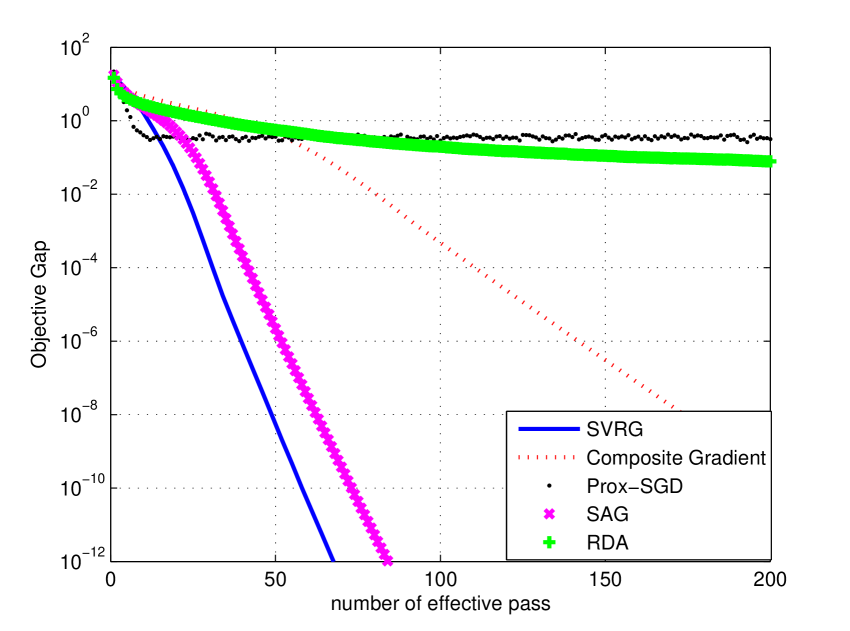
(a) r=50,b=0

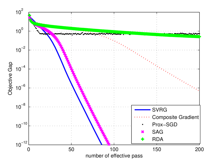
(b) r=100,b=0

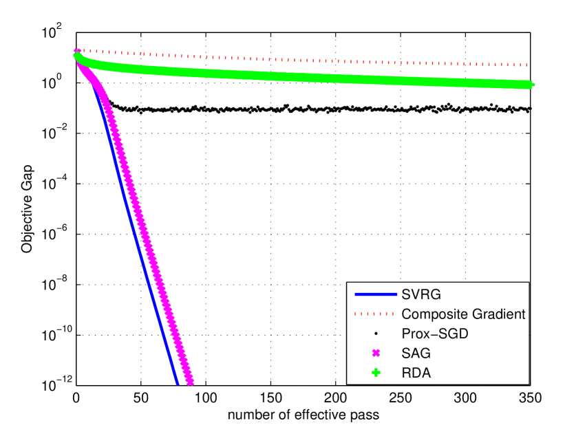
(c) r=50,b=0.1

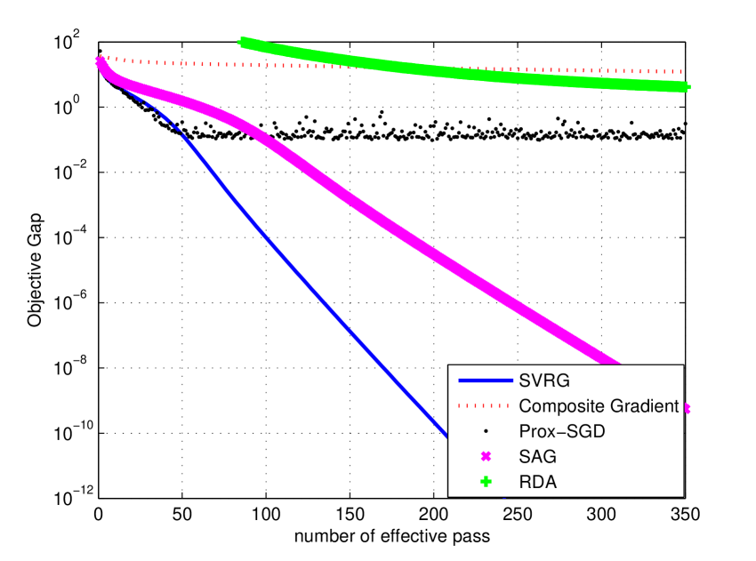
(d) r=100,b=0.4

Figure 1: Comparison between five algorithms on Lasso. The x-axis is the number of pass over the dataset. y-axis is the objective gap $G(\theta_{k})-G(\hat{\theta})$ with a log scale. In figure (a), r=50,b=0 . In figure (b), r=100,b=0. In figure (c), r=50,b=0.1. In figure (d), r=100,b=0.4 .

In Figure 1, for different values of $r$ and $b$, we report the objective gap $G(\theta_{k})-G(\hat{\theta})$ versus the number of passes of the dataset for the algorithms mentioned above. We evaluate $G(\hat{\theta})$ by running SVRG long enough (more than 500 effective passes). Clearly the objective gap of SVRG decreases geometrically, which validates our theoretic findings. We also observe that when $r$ is larger, SVRG converges slower, compared with smaller $r$. This agrees with our theorem, as $r$ affects the value of $\bar{\sigma}$ and hence the contraction factor $\alpha$. In particular, small $r$ leads to small $\alpha$ thus the algorithm enjoys a faster convergence speed. The composite gradient method, which uses full information at each iteration, converges linearly in (a) and (b) but with a slower rate. This agrees with the common phenomenon that stochastic variance reduction methods typically converges faster (w.r.t. the number of passes of datasets). In (c) and (d), its performance deteriorate significantly due to the large condition number when $b$ is not zero. The optimality gaps of SGD and RDA decrease slowly, indicating lack of linear convergence, due to large variance of gradients. We make one interesting observation about SAG: it has a similar performance to that of SVRG in our setting, strongly suggesting that it may be possible to establish linear convergence of SAG under the RSC condition. However, we stress that the goal of the experiments is to validate our analysis of SVRG, rather than comparing SVRG with SAG.

4.1.2 Group Lasso

We now report results on group sparsity case, in particular the empirical performance of different algorithms to solve Group Lasso. Similar to the above example, we have $p=5000$ and $n=2500$ and each feature is generated from the normal distribution $N(0,\Sigma)$, where $\Sigma_{ii}=1$ and $\Sigma_{ij}=b,i\neq j.$ The cardinality of the non-zero group is $s_{\mathcal{G}}$, and the size of each group is $q$ . In Figure 2, we report results on different settings of cardinality $s_{\mathcal{G}}$ and the covariance matrix $\Sigma$ and $q$.

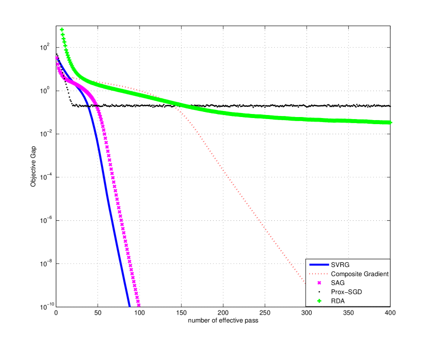
(a) $s_{\mathcal{G}}$=10,q=10, b=0

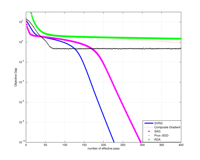
(b) $s_{\mathcal{G}}$=20, q=20, b=0

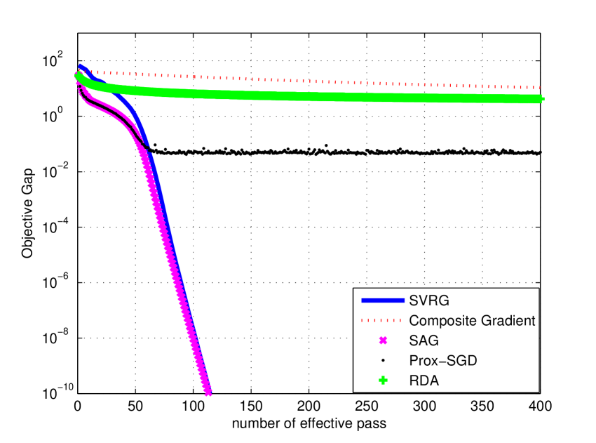
(c) $s_{\mathcal{G}}$=10, q=10, b=0.1

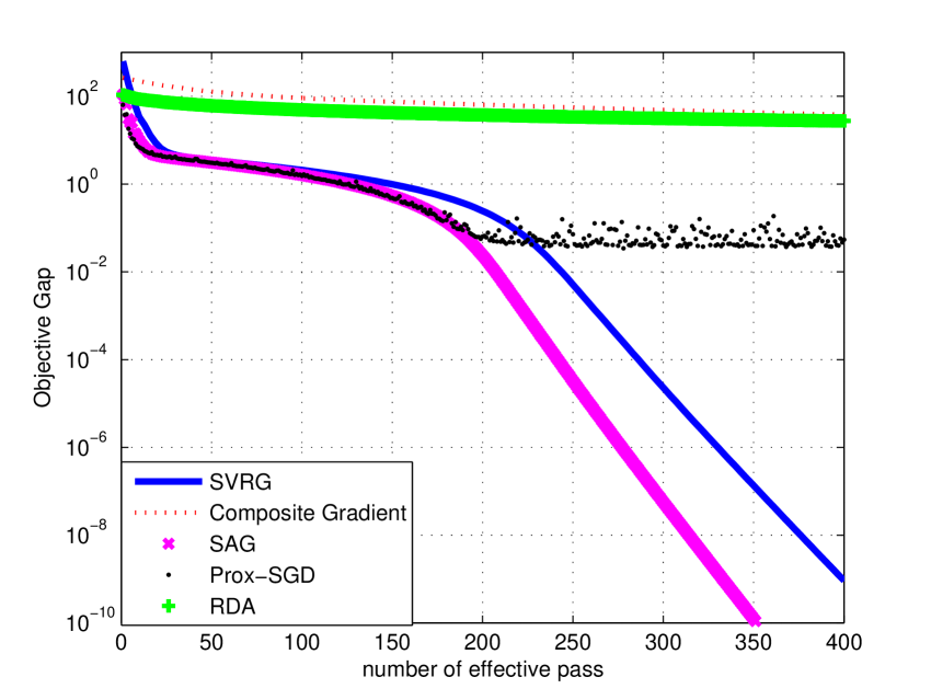
(d) $s_{\mathcal{G}}$=20, q=20, b=0.4

Figure 2: Comparison between five algorithms on group Lasso. The x-axis is the number of pass over the dataset. y-axis is the objective gap $G(\theta_{k})-G(\hat{\theta})$ with log scale. In figure (a), $s_{\mathcal{G}}$=10, q=10, b=0 . In figure (b), $s_{\mathcal{G}}$=20, q=20, b=0. In figure (c), $s_{\mathcal{G}}$=10, q=10, b=0.1. In figure (d), $s_{\mathcal{G}}$=20, q=20, b=0.4 .

In (a), similar to the Lasso case, SVRG and SAG converge with linear rates, and have similar performance. On the other hand, SGD and RDA converge slowly due to the variance of the gradient. In (b), we observe that composite gradient method converge much slower. It is possibly because the contraction factor of composite gradient method is close to 1 in this setting as the $\theta^{*}$ becomes less sparse. In (c) and (d) the composite gradient method does not work due to the large condition number.

4.1.3 Corrected Lasso

We generate data as follows: $y_{i}=x_{i}^{T}\theta^{*}+\xi_{i}$, where each data point $x_{i}\in\mathbb{R}^{p}$ is drawn from normal distribution $N(0,I)$, and the noise $\xi_{i}$ is drawn from $N(0,1)$. The coefficient $\theta^{*}$ is sparse with cardinality $r$, where the non-zero coefficient equals to $\pm 1$ generated from the Bernoulli distribution with parameter $0.5$. We set covariance matrix $\Sigma_{w}=\gamma_{w}I$. We choose $\lambda=0.05$ in the formulation. The result is presented in Figure 3.

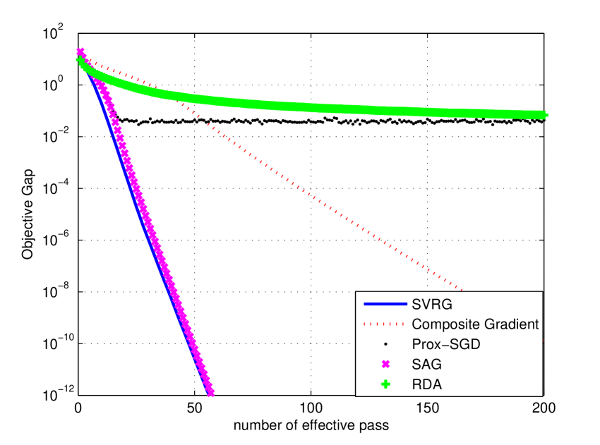
(a) $n=2500,p=3000,r=50,\gamma_{w}=0.05$

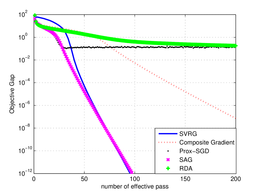
(b) $n=2500,p=5000,r=100,\gamma_{w}=0.1$

Figure 3: Results on Corrected Lasso. The x-axis is the number of pass over the dataset. y-axis is the objective gap $G(\theta_{k})-G(\hat{\theta})$ with log scale. We try two different settings. In the first figure $n=2500,p=3000,r=50,\gamma_{w}=0.05$.in the second figure $n=2500,p=5000,r=100,\gamma_{w}=0.1$.

In both figures (a) and (b), SVRG, SAG and Composite gradient converge linearly. According to our theory, as $\bar{\sigma}$ in figure (a) is larger than that in figure (b), and $\frac{\gamma_{w}}{\bar{\sigma}}$ in figure (a) is smaller than that in (b), SVRG should converge faster in the setting of figure (a), which matches our simulation result. SGD and RDA have large optimality gaps.

4.1.4 SCAD

The way to generate data is same with Lasso. Here $x_{i}\in\mathbb{R}^{p}$ is drawn from normal distribution $N(0,2I)$ (Here We choose $2I$ to satisfy the requirement of $\bar{\sigma}$ and $\mu$ in our Theorem, although if we choose $N(0,I)$, the algorithm still works. ). $\lambda=0.05$ in the formulation. We present the result in Figure 4, for two settings on $n$, $p$, $r$, $\zeta$. Note that $\bar{\sigma}\geq 0.5$ and $\frac{1}{\zeta-1}\leq 0.5$ in both cases, thus our theorem asserts that SVRG converge linearly under appropriate choices of $\beta$ and $m$.

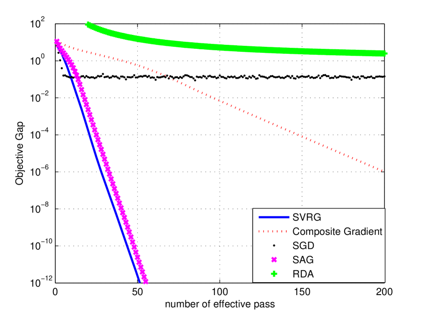
(a) $n=3000,p=2500,r=30,\zeta=4.5$

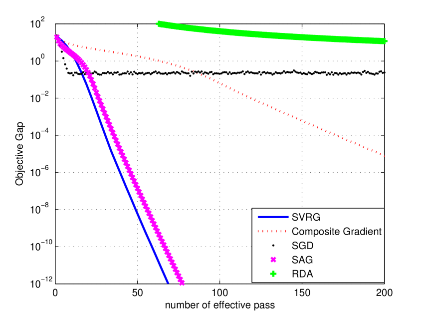
(b) $n=2500,p=5000,r=50,\zeta=3.7$

Figure 4: Results on SCAD. The x-axis is the number of pass over the dataset. y-axis is the objective gap $G(\theta_{k})-G(\hat{\theta})$ with log scale.

We observe from Figure 4 that in both cases, SVRG, SAG converges with linear rates and have similar performance. The composite gradient method also converges linearly but with a slower speed. SGD and RDA have large optimality gaps.

4.2 Real data

This section presents results of several numerical experiments on real datasets.

4.2.1 Sparse classification problem

The first problem we consider is sparse classification. In particular, we apply logistic regression with $l_{1}$ regularization on rcv1 ($n=20242,d=47236$) Lewis et al. (2004) and sido0 ($n=12678,d=4932$) Guyon (2008) datasets for the binary classification problem, i.e.,

$$G(\theta)=\frac{1}{n}\sum_{i=1}^{n}\log(1+\exp(-y_{i}\langle x_{i},\theta\rangle)+\lambda\|\theta\|_{1}.$$

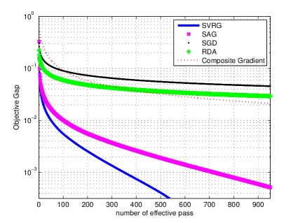
Figure 5: Different methods on rcv1 dataset.

We choose $\lambda=2\cdot 10^{-5}$ in rcv1 dataset and $\lambda=10^{-4}$ in sido0 dataset suggested in Xiao and Zhang (2014).

Figure 5 shows the performance of five algorithms on rcv1 dataset. The x-axis is the number of passes over the dataset, and the y-axis is the optimality gap in log-scale. In the experiment we choose $m=2n$ for SVRG. Among all five algorithms, SVRG performs best followed by SAG. The composite gradient method does not perform well in this dataset. RDA and SGD converge slowly and the error of them remains large even after 1000 passes of the entire dataset.

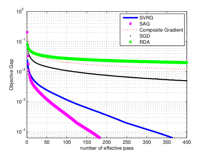
Figure 6: Different methods on sido0 dataset.

Figure 6 reports results on sido0 dataset. On this dataset, SAG outperforms SVRG. We also observe that SGD outperforms composite gradient. The RDA converges with the slowest rate.

4.2.2 Group sparse regression

We consider a group sparse regression problem on the Boston Housing dataset Harrison and Rubinfeld (2013). As suggested in Swirszcz et al. (2009); Xiang et al. (2014), to take into account the non-linear relationship between variables and the response, up to third-degree polynomial expansion is applied on each feature. In particular, terms $x$, $x^{2}$ and $x^{3}$ are grouped together. We consider group Lasso model on this problem with $\lambda=0.1$. We choose the setting $m=2n$ in SVRG.

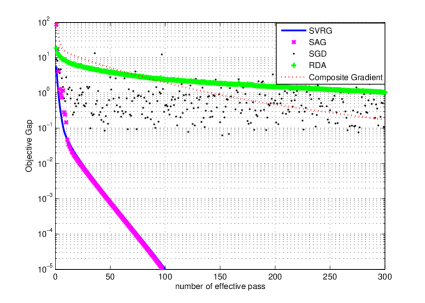
Figure 7: Five different algorithms on Boston Housing dataset.

In Figure 7, we show the objective gap of various algorithms versus the number of passes over the dataset. SVRG and SAG have almost identical performance. SGD fails to converge – the optimality gap oscillates between 0.1 and 1. Both the composite gradient method and RDA converge slowly.

5 Conclusion and future work

In this paper, we analyzed a state-of-art stochastic first order optimization algorithm SVRG where the objective function is not strongly convex, or even non-convex. We established linear convergence of SVRG exploiting the concept of restricted strong convexity. Our setup naturally includes several important statistical models such as Lasso, group sparse regression and SCAD, to name a few. We further validated our theoretic findings with numerical experiments on synthetic and real datasets.

Appendix A Phase transition of linear rate and sub-linear rate in Lasso

We generate data as follows: $y_{i}=x_{i}^{T}\theta^{*}+\xi_{i}$, where each data point $x_{i}\in\mathbb{R}^{p}$ is drawn from normal distribution $N(0,I)$, and the noise $\xi_{i}$ is drawn from $N(0,1)$. The coefficient $\theta^{*}$ is sparse with cardinality $r$, where the non-zero coefficient equals to $\pm 1$ generated from the Bernoulli distribution with probability $0.5$. The sample size is $n=2500$, and the dimension of problem is $p=5000$.

In Figure 8, we increase $r$ from 500 to 1500 and plot the convergence rate of SVRG. We observe a phase transition from linear convergence to sublinear convergence happening between $r=750$ and $r=1000$. This phenomena is captured by our theorem: When $r$ is too large, the requirement $\bar{\sigma}=\frac{1}{2}\sigma_{\min}(\Sigma)-c_{1}\nu(\Sigma)\frac{r\log p}{n}\geq 0$ breaks.

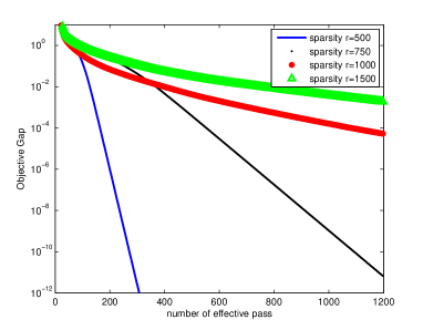
Figure 8: Phase transition of linear rate. The x-axis is the number of pass over the dataset. y-axis is the objective gap $G(\theta_{k})-G(\hat{\theta})$ with log scale.

Appendix B Proofs

We provide in this section proofs to all results presented.

B.1 SVRG with convex objective function

Remind the objective function we aim to optimize is

$$\begin{split}\min_{\psi(\theta)\leq\rho}F(\theta)+\lambda\psi(\theta)=\frac{1}{n}\sum_{i=1}^{n}f_{i}(\theta)+\lambda\psi(\theta).\end{split}$$ (9)

We denote

$$\hat{\theta}=\arg\min_{\psi(\theta)\leq\rho}F(\theta)+\lambda\psi(\theta).$$

The following technical lemma is well-known in SVRG to bound the variance of the modified stochastic gradient $v_{k}$. It is indeed Corollary 3 in Xiao and Zhang (2014), which we present here for completeness.

Lemma 1.

Consider $v_{k-1}$ defined in the algorithm 1. Conditioned on $\theta_{k-1}$, we have $\mathbb{E}v_{k-1}=\nabla F(\theta_{k-1})$, and

$$\mathbb{E}\|v_{k-1}-\nabla F(\theta_{k-1})\|_{2}^{2}\leq 4L[G(\theta_{k-1})-G(\hat{\theta})+G(\tilde{\theta})-G(\hat{\theta})].$$

Lemma 2.

Suppose that $F(\theta)$ is convex and $\psi(\theta)$ is decomposable with respect to $(M,\bar{M})$, if we choose $\lambda\geq 2\psi^{*}(\nabla F(\theta^{*}))$, $\psi(\theta^{*})\leq\rho$ , define the error $\Delta^{*}=\hat{\theta}-\theta^{*}$, then we have the following condition holds,

$$\psi(\Delta^{*}_{\bar{M}^{\perp}})\leq 3\psi(\Delta^{*}_{\bar{M}})+4\psi(\theta^{*}_{M^{\perp}}),$$

which further implies $\psi(\Delta^{*})\leq\psi(\Delta^{*}_{\bar{M}^{\perp}})+\psi(\Delta^{*}_{\bar{M}})\leq 4\psi(\Delta^{*}_{\bar{M}})+4\psi(\theta^{*}_{M^{\perp}}).$

Proof.

Using the optimality of $\hat{\theta}$, we have

$$F(\hat{\theta})+\lambda\psi(\hat{\theta})-F(\theta^{*})-\lambda\psi(\theta^{*})\leq 0.$$

So we have

$$\lambda\psi(\theta^{*})-\lambda\psi(\hat{\theta})\geq F(\hat{\theta})-F(\theta^{*})\geq\langle\nabla F(\theta^{*}),\hat{\theta}-\theta^{*}\rangle\geq-\psi^{*}(\nabla F(\theta^{*}))\psi(\Delta^{*}),$$

where the second inequality holds from the convexity of $F(\theta)$, and the third holds using Holder inequality.

Using triangle inequality, we have

$$\psi(\Delta^{*})\leq\psi(\Delta^{*}_{\bar{M}})+\psi(\Delta^{*}_{\bar{M}^{\perp}}).$$

So

$$\lambda\psi(\theta^{*})-\lambda\psi(\hat{\theta})\geq-\psi^{*}(\nabla F(\theta^{*}))(\psi(\Delta^{*}_{\bar{M}})+\psi(\Delta^{*}_{\bar{M}^{\perp}}))$$ (10)

Notice

$$\hat{\theta}=\theta^{*}+\Delta^{*}=\theta^{*}_{M}+\theta^{*}_{M^{\perp}}+\Delta^{*}_{\bar{M}}+\Delta^{*}_{\bar{M}^{\perp}},$$

which leads to

$$\begin{split}\psi(\hat{\theta})-\psi(\theta^{*})&\overset{(a)}{\geq}\psi(\theta^{*}_{M}+\Delta^{*}_{\bar{M}^{\perp}})-\psi(\theta^{*}_{M^{\perp}})-\psi(\Delta^{*}_{\bar{M}})-\psi(\theta^{*})\\ &\overset{(b)}{=}\psi(\theta^{*}_{M})+\psi(\Delta^{*}_{\bar{M}^{\perp}})-\psi(\theta^{*}_{M^{\perp}})-\psi(\Delta^{*}_{\bar{M}})-\psi(\theta^{*})\\ &\overset{(c)}{\geq}\psi(\theta^{*}_{M})+\psi(\Delta^{*}_{\bar{M}^{\perp}})-\psi(\theta^{*}_{M^{\perp}})-\psi(\Delta^{*}_{\bar{M}})-\psi(\theta^{*}_{M})-\psi(\theta^{*}_{M^{\perp}})\\ &\geq\psi(\Delta^{*}_{\bar{M}^{\perp}})-2\psi(\theta^{*}_{M^{\perp}})-\psi(\Delta^{*}_{\bar{M}}),\end{split}$$ (11)

where $(a)$ and $(c)$ holds from the triangle inequality, $(b)$ uses the decomposability of $\psi(\cdot)$.

Substitute left hand side of 10 by above result and use the assumption that $\lambda\geq 2\psi^{*}(\nabla F(\theta^{*}))$, we have

$$-\frac{\lambda}{2}(\psi(\Delta^{*}_{\bar{M}})+\psi(\Delta^{*}_{\bar{M}^{\perp}}))+\lambda(\psi(\Delta^{*}_{\bar{M}^{\perp}})-2\psi(\theta^{*}_{M^{\perp}})-\psi(\Delta^{*}_{\bar{M}}))\leq 0$$

which implies

$$\psi(\Delta^{*}_{\bar{M}^{\perp}})\leq 3\psi(\Delta^{*}_{\bar{M}})+4\psi(\theta^{*}_{M^{\perp}}).$$

∎

Lemma 3.

$F(\theta)$ is convex and $\psi(\theta)$ is decomposable with respect to $(M,\bar{M})$, if we choose $\lambda\geq 2\psi^{*}(\nabla F(\theta^{*}))$, $\psi(\theta^{*})\leq\rho$ and suppose there exist a time step $S>0$ and a given tolerance $\epsilon^{\prime}$ such that for all $s>S$, $G(\theta^{s})-G(\hat{\theta})\leq\epsilon^{\prime}$ holds, then for the error $\Delta^{s}=\theta^{s}-\theta^{*}$ we have

$$\psi(\Delta^{s}_{\bar{M}^{\perp}})\leq 3\psi(\Delta^{s}_{\bar{M}})+4\psi(\theta^{*}_{M^{\perp}})+2\min\{\frac{\epsilon^{\prime}}{\lambda},\rho\},$$

which implies

$$\psi(\Delta^{s})\leq 4\psi(\Delta^{s}_{\bar{M}})+4\psi(\theta^{*}_{M^{\perp}})+2\min\{\frac{\epsilon^{\prime}}{\lambda},\rho\}.$$

Proof.

First notice $G(\theta^{s})-G(\theta^{*})\leq\epsilon^{\prime}$ holds by assumption since $G(\theta^{*})\geq G(\hat{\theta}).$ So we have

$$F(\theta^{s})+\lambda\psi(\theta^{s})-F(\theta^{*})-\lambda\psi(\theta^{*})\leq\epsilon^{\prime}.$$

Follow same steps in the proof of Lemma 2, we have

$$\psi(\Delta^{s}_{\bar{M}^{\perp}})\leq 3\psi(\Delta^{s}_{\bar{M}})+4\psi(\theta^{*}_{M^{\perp}})+2\frac{\epsilon^{\prime}}{\lambda}.$$

Notice $\Delta^{s}=\Delta^{s}_{\bar{M}^{\perp}}+\Delta^{s}_{\bar{M}}$ so $\psi(\Delta^{s}_{\bar{M}^{\perp}})\leq\psi(\Delta^{s}_{\bar{M}})+\psi(\Delta^{s})$ using the triangle inequality.
Then use the fact that $\psi(\Delta^{s})\leq\psi(\theta^{*})+\psi(\theta^{s})\leq 2\rho$, we establish

$$\psi(\Delta^{s}_{\bar{M}^{\perp}})\leq 3\psi(\Delta^{s}_{\bar{M}})+4\psi(\theta^{*}_{M^{\perp}})+2\min\{\frac{\epsilon^{\prime}}{\lambda},\rho\}.$$

The second statement follows immediately from $\psi(\Delta^{s})\leq\psi(\Delta^{s}_{\bar{M}^{\perp}})+\psi(\Delta^{s}_{\bar{M}})$. ∎

Using the above two lemmas we now prove modified restricted convexity on $G(\theta^{s})-G(\hat{\theta})$.

Lemma 4.

Under the same assumptions of Lemma 3, we have

$$G(\theta^{s})-G(\hat{\theta})\geq\left(\frac{\sigma}{2}-32\tau_{\sigma}H^{2}(\bar{M})\right)\|\hat{\Delta}^{s}\|_{2}^{2}-\epsilon^{2}(\Delta^{*},M,\bar{M}),$$ (12)

where $\epsilon^{2}(\Delta^{*},M,\bar{M})=2\tau_{\sigma}(\delta_{stat}+\delta)^{2}$, $\delta=2\min\{\frac{\epsilon^{\prime}}{\lambda},\rho\}$, and $\delta_{stat}=H(\bar{M})\|\Delta^{*}\|_{2}+8\psi(\theta^{*}_{M^{\perp}})$.

Proof.

At the beginning of the proof, we show a simple fact on $\hat{\Delta}^{s}=\theta^{s}-\hat{\theta}$. Notice the conclusion in Lemma 3 is on $\Delta^{s}$, we need transfer it to $\hat{\Delta}^{s}$.

$$\begin{split}\psi(\hat{\Delta}^{s})&\leq\psi(\Delta^{s})+\psi(\Delta^{*})\\ &\leq 4\psi(\Delta^{s}_{\bar{M}})+4\psi(\theta^{*}_{M^{\perp}})+2\min\{\frac{\epsilon^{\prime}}{\lambda},\rho\}+4\psi(\Delta^{*}_{\bar{M}})+4\psi(\theta^{*}_{M^{\perp}})\\ &\leq 4H(\bar{M})\|\Delta^{s}\|_{2}+4H(\bar{M})\|\Delta^{*}\|_{2}+8\psi(\theta^{*}_{M^{\perp}})+2\min\{\frac{\epsilon^{\prime}}{\lambda},\rho\},\end{split}$$ (13)

where the first inequality holds from the triangle inequality, the second inequality uses Lemma 2 and 3, the third holds because of the definition of subspace compatibility.

We now use the above result to rewrite the RSC condition. We know

$$F(\theta^{s})-F(\hat{\theta})-\langle\nabla F(\hat{\theta}),\hat{\Delta}^{s}\rangle\geq\frac{\sigma}{2}\|\hat{\Delta}^{s}\|_{2}^{2}-\tau_{\sigma}\psi^{2}(\hat{\Delta}^{s})$$

which implies $G(\theta^{s})-G(\hat{\theta})\geq\frac{\sigma}{2}\|\hat{\Delta}^{s}\|_{2}^{2}-\tau_{\sigma}\psi^{2}(\hat{\Delta}^{s})$, by using the fact that $\hat{\theta}$ is the optimal solution to the problem 2 and $\phi(\cdot)$ is convex. Notice that

$$\begin{split}\psi(\hat{\Delta}^{s})&\leq 4H(\bar{M})\|\Delta^{s}\|_{2}+4H(\bar{M})\|\Delta^{*}\|_{2}+8\psi(\theta^{*}_{M^{\perp}})+2\min\{\frac{\epsilon^{\prime}}{\lambda},\rho\}\\ &\leq 4H(\bar{M})\|\hat{\Delta}^{s}\|_{2}+8H(\bar{M})\|\Delta^{*}\|_{2}+8\psi(\theta^{*}_{M^{\perp}})+2\min\{\frac{\epsilon^{\prime}}{\lambda},\rho\},\end{split}$$ (14)

where the second inequality uses the triangle inequality. Now use the inequality $(a+b)^{2}\leq 2a^{2}+2b^{2}$, we upper bound $\psi^{2}(\hat{\Delta}^{s})$ with

$$\psi^{2}(\hat{\Delta}^{s})\leq 32H^{2}(\bar{M})\|\hat{\Delta}^{s}\|_{2}^{2}+2\left(8H(\bar{M})\|\Delta^{*}\|_{2}+8\psi(\theta^{*}_{M^{\perp}})+2\min\{\frac{\epsilon^{\prime}}{\lambda},\rho\}\right)^{2}.$$

Substitute this upper bound into RSC, we have

$$G(\theta^{s})-G(\hat{\theta})\geq\left(\frac{\sigma}{2}-32\tau_{\sigma}H^{2}(\bar{M})\right)\|\hat{\Delta}^{s}\|_{2}^{2}-2\tau_{\sigma}\left(8H(\bar{M})\|\Delta^{*}\|_{2}+8\psi(\theta^{*}_{M^{\perp}})+2\min\{\frac{\epsilon^{\prime}}{\lambda},\rho\}\right)^{2}.$$

Notice that by $\delta=2\min\{\frac{\epsilon^{\prime}}{\lambda},\rho\}$, $\delta_{stat}=H(\bar{M})\|\Delta^{*}\|_{2}+8\psi(\theta^{*}_{M^{\perp}}),$ and $\epsilon^{2}(\Delta^{*},M,\bar{M})=2\tau_{\sigma}(\delta_{stat}+\delta)^{2}$, we have

$$\epsilon^{2}(\Delta^{*},M,\bar{M})=2\tau_{\sigma}\left(8H(\bar{M})\|\Delta^{*}\|_{2}+8\psi(\theta^{*}_{M^{\perp}})+2\min\{\frac{\epsilon^{\prime}}{\lambda},\rho\}\right)^{2}.$$

We thus conclude

$$G(\theta^{s})-G(\hat{\theta})\geq\left(\frac{\sigma}{2}-32\tau_{\sigma}H^{2}(\bar{M})\right)\|\hat{\Delta}^{s}\|_{2}^{2}-\epsilon^{2}(\Delta^{*},M,\bar{M}).$$ (15)

∎

The next lemma is a simple extension of a standard property proximal operator with a constraint $\Omega$.

Lemma 5.

Define $prox_{h,\Omega}(x)=\arg\min_{z\in\Omega}h(z)+\frac{1}{2}\|z-x\|_{2}^{2}$, where $\Omega$ is a convex compact set, then $\|prox_{h,\Omega}(x)-prox_{h,\Omega}(y)\|_{2}\leq\|x-y\|_{2}.$

Proof.

Define $u=prox_{h,\Omega}(x)$ and $v=prox_{h,\Omega}(y)$. Using optimality of $u$ we have

$$\langle\partial h(u)+u-x,\tilde{u}-u\rangle\geq 0\quad\forall\tilde{u}\in\Omega.$$

We choose $\tilde{u}=v$ and obtain $\langle\partial h(u)+u-x,v-u\rangle\geq 0.$ Similarly we have $\langle\partial h(v)+v-y,u-v\rangle\geq 0.$ Summing up these two inequalities leads to

$$\langle v-y-u+x,u-v\rangle\geq\langle\partial h(u)-\partial h(v),u-v\rangle\geq 0,$$

where the second inequality is due to convexity of $h(\cdot)$. This leads to

$$\|prox_{h,\Omega}(x)-prox_{h,\Omega}(y)\|_{2}^{2} \leq \langle prox_{h,\Omega}(x)-prox_{h,\Omega}(y),x-y\rangle$$

$$\stackrel{{\scriptstyle(a)}}{{\leq}} \|prox_{h,\Omega}(x)-prox_{h,\Omega}(y)\|_{2}\|x-y\|_{2},$$

which implies the lemma. Here (a) holds by Cauchy-Schwarz inequality. ∎

Lemma 6.

Under the same assumption of Lemma 3, and suppose that $\bar{\sigma}=\sigma-64\tau_{\sigma}H^{2}(\bar{M})>0$, $\alpha=\frac{1}{\beta(1-4L\beta)m\bar{\sigma}}+\frac{4L\beta(m+1)}{(1-4L\beta)m}<1$ we have

$$\mathbb{E}G(\theta^{s+1})-G(\hat{\theta})\leq\alpha(G(\theta^{s})-G(\hat{\theta}))+\frac{1}{\bar{\sigma}\beta(1-4L\beta)m}{\epsilon}^{2}(\Delta^{*},M,\bar{M}).$$

Notice this lemma states that the optimization error decrease by a fraction $\alpha$ plus some additional term related to $\epsilon^{2}(\Delta^{*},M,\bar{M})$. We emphasize that we make no assumption of strong convexity.

Proof.

In the following proof we denote $\psi_{\lambda}(\theta)\triangleq\lambda\psi(\theta)$. In stage $s+1$, we have

$$\begin{split}&G(\theta_{k+1})-G(\hat{\theta})\\ \leq&F(\theta_{k})-F(\hat{\theta})+\langle\nabla F(\theta_{k}),\theta_{k+1}-\theta_{k}\rangle+\frac{L}{2}\|\theta_{k+1}-\theta_{k}\|_{2}^{2}+\psi_{\lambda}(\theta_{k+1})-\psi_{\lambda}(\hat{\theta})\\ \leq&\langle\nabla F(\theta_{k}),\theta_{k}-\hat{\theta}\rangle+\langle\nabla F(\theta_{k}),\theta_{k+1}-\theta_{k}\rangle+\langle\partial\psi_{\lambda}(\theta_{k+1}),\theta_{k+1}-\hat{\theta}\rangle+\frac{L}{2}\|\theta_{k+1}-\theta_{k}\|_{2}^{2}\\ =&\langle\nabla F(\theta_{k}),\theta_{k+1}-\hat{\theta}\rangle+\langle\partial\psi_{\lambda}(\theta_{k+1}),\theta_{k+1}-\hat{\theta}\rangle+\frac{L}{2}\|\theta_{k+1}-\theta_{k}\|_{2}^{2},\end{split}$$ (16)

where we use smoothness assumption of $F(\theta)$ in the first inequality, and the second inequality holds from the convexity of $F(\theta)$ and $\psi(\theta)$. Now using optimality condition of $\theta_{k+1}$, we obtain

$$\langle\theta_{k+1}-(\theta_{k}-\beta v_{k})+\beta\partial\psi_{\lambda}(\theta_{k+1}),\theta-\theta_{k+1}\rangle\geq 0,~{}~{}\forall\theta\in\{\theta|\psi(\theta)\leq\eta\}.$$

We choose $\theta=\hat{\theta}$ and get

$$\langle\theta_{k+1}-(\theta_{k}-\beta v_{k})+\beta\partial\psi_{\lambda}(\theta_{k+1}),\hat{\theta}-\theta_{k+1}\rangle\geq 0,$$

$$\Longrightarrow \langle\partial\psi_{\lambda}(\theta_{k+1}),\theta_{k+1}-\hat{\theta}\rangle\leq\langle\frac{1}{\beta}(\theta_{k+1}-\theta_{k})+v_{k},\hat{\theta}-\theta_{k+1}\rangle.$$

Substitute the above inequality to Equation (16), we have

$$\begin{split}G(\theta_{k+1})-G(\hat{\theta})&\leq\langle\nabla F(\theta_{k}),\theta_{k+1}-\hat{\theta}\rangle+\langle\frac{1}{\beta}(\theta_{k+1}-\theta_{k})+v_{k},\hat{\theta}-\theta_{k+1}\rangle+\frac{L}{2}\|\theta_{k+1}-\theta_{k}\|_{2}^{2}\\ &=\langle\nabla F(\theta_{k})-v_{k},\theta_{k+1}-\hat{\theta}\rangle+\frac{1}{\beta}\langle\theta_{k+1}-\theta_{k},\hat{\theta}-\theta_{k}\rangle+(\frac{L}{2}-\frac{1}{\beta})\|\theta_{k+1}-\theta_{k}\|_{2}^{2}\\ &\leq\langle\nabla F(\theta_{k})-v_{k},\theta_{k+1}-\hat{\theta}\rangle+\frac{1}{\beta}\langle\theta_{k+1}-\theta_{k},\hat{\theta}-\theta_{k}\rangle-\frac{1}{2\beta}\|\theta_{k+1}-\theta_{k}\|_{2}^{2},\end{split}$$ (17)

where the last inequality holds using the fact that $0\leq\beta\leq\frac{1}{L}$.

Define $\bar{\theta}_{k+1}=prox_{\beta\psi_{\lambda},\Omega}(\theta_{k}-\beta\nabla F(\theta_{k}))$

$$\begin{split}&\|\theta_{k+1}-\hat{\theta}\|_{2}^{2}\\ =&\|\theta_{k}-\hat{\theta}\|_{2}^{2}+2\langle\theta_{k+1}-\theta_{k},\theta_{k}-\hat{\theta}\rangle+\|\theta_{k+1}-\theta_{k}\|_{2}^{2}\\ \leq&\|\theta_{k}-\hat{\theta}\|_{2}^{2}+2\beta\langle\nabla F(\theta_{k})-v_{k},\theta_{k+1}-\hat{\theta}\rangle+2\beta(G(\hat{\theta})-G(\theta_{k+1}))\\ \leq&\|\theta_{k}-\hat{\theta}\|_{2}^{2}+2\beta(G(\hat{\theta})-G(\theta_{k+1}))\\ &\qquad+2\beta\langle\nabla F(\theta_{k})-v_{k},\theta_{k+1}-\bar{\theta}_{k+1}\rangle+2\beta\langle\nabla F(\theta_{k})-v_{k},\bar{\theta}_{k+1}-\hat{\theta}\rangle\\ \leq&\|\theta_{k}-\hat{\theta}\|_{2}^{2}+2\beta(G(\hat{\theta})-G(\theta_{k+1}))+2\beta\|\nabla F(\theta_{k})-v_{k}\|_{2}\|\theta_{k+1}-\bar{\theta}_{k+1}\|_{2}\\ &\qquad+2\beta\langle\nabla F(\theta_{k})-v_{k},\bar{\theta}_{k+1}-\hat{\theta}\rangle\\ \leq&\|\theta_{k}-\hat{\theta}\|_{2}^{2}+2\beta(G(\hat{\theta})-G(\theta_{k+1}))+2\beta^{2}\|\nabla F(\theta_{k})-v_{k}\|_{2}^{2}+2\beta\langle\nabla F(\theta_{k})-v_{k},\bar{\theta}_{k+1}-\hat{\theta}\rangle\end{split}$$ (18)

where the first inequality uses Equation (17), and the last inequality uses the below equation implied by Lemma 5

$$\|\theta_{k+1}-\bar{\theta}_{k+1}\|_{2}\leq\|\theta_{k}-\beta v_{k}-(\theta_{k}-\beta\nabla F(\theta_{k-1}))\|_{2}.$$

Now, take expectation at both side w.r.t. $i_{k}$, and apply Lemma 1 on $\mathbb{E}\|\nabla F(\theta_{k})-v_{k}\|_{2}^{2}$ and notice the fact that $\mathbb{E}\langle\nabla F(\theta_{k})-v_{k},\bar{\theta}_{k+1}-\hat{\theta}\rangle=0$, we have

$$\mathbb{E}\|\theta_{k+1}-\hat{\theta}\|_{2}^{2}\leq\|\theta_{k}-\hat{\theta}\|_{2}^{2}+\beta(G(\hat{\theta})-\mathbb{E}G(\theta_{k+1}))+8L\beta^{2}(G(\theta_{k})-G(\hat{\theta})+G(\tilde{\theta})-G(\hat{\theta})).$$

In stage $s$, sum up the above inequality at both side and take expectation, and use the fact that $\tilde{\theta}=\theta^{s}$ we have

$$2\beta(1-4L\beta)\sum_{k=1}^{m}(\mathbb{E}G(\theta_{k})-G(\hat{\theta}))\leq\|\theta^{s}-\hat{\theta}\|_{2}^{2}+8L\beta^{2}(m+1)[G(\theta^{s})-G(\hat{\theta})].$$

One the left hand side, we use the convexity of $G(\theta)$, i.e.,

$$m(\mathbb{E}G(\theta^{s+1})-G(\hat{\theta}))\leq\sum_{k=1}^{m}(\mathbb{E}G(\theta_{k})-G(\hat{\theta})).$$

We apply Equation (12) on the right hand side, i.e.,

$$G(\theta^{s})-G(\hat{\theta})\geq(\frac{\sigma}{2}-32\tau_{\sigma}H^{2}(\bar{M}))\|\hat{\Delta}^{s}\|_{2}^{2}-\epsilon^{2}(\Delta^{*},M,\bar{M}).$$

Recall the definition $\bar{\sigma}=\sigma-64\tau_{\sigma}H^{2}(\bar{M})$, we have

$$G(\theta^{s})-G(\hat{\theta})\geq\frac{\bar{\sigma}}{2}\|\hat{\Delta}^{s}\|_{2}^{2}-\epsilon^{2}(\Delta^{*},M,\bar{M}).$$

Hence we have

$$2\beta(1-4L\beta)m(\mathbb{E}G(\theta^{s+1})-G(\hat{\theta}))\leq\frac{G(\theta^{s})-G(\hat{\theta})+\epsilon^{2}(\Delta^{*},M,\bar{M})}{\bar{\sigma}/2}+8L\beta^{2}(m+1)[G(\tilde{\theta}^{s})-G(\hat{\theta})].$$

Rearrange terms in the above inequality we have

$$\begin{split}\mathbb{E}G(\theta^{s+1})-G(\hat{\theta})&\leq(\frac{1}{\beta(1-4L\beta)m\bar{\sigma}}+\frac{4L\beta(m+1)}{(1-4L\beta)m})[G(\theta^{s})-G(\hat{\theta})]\\ &\qquad+\frac{\epsilon^{2}(\Delta^{*},M,\bar{M})}{\bar{\sigma}\beta(1-4L\beta)m}\end{split}$$ (19)

Remind the definition of $\alpha$, this leads to

$$\mathbb{E}G(\theta^{s+1})-G(\hat{\theta})\leq\alpha(G(\theta^{s})-G(\hat{\theta}))+\frac{1}{\bar{\sigma}\beta(1-4L\beta)m}{\epsilon}^{2}(\Delta^{*},M,\bar{M}).$$

∎

We can iteratively apply above inequality from time step S to s, we have

$$\begin{split}\mathbb{E}G(\theta^{s})-G(\hat{\theta})\leq&\alpha^{s-S}(G(\theta^{S})-G(\hat{\theta}))+\frac{\sum_{i=0}^{s-S}\alpha^{i}}{\bar{\sigma}\beta(1-4L\beta)m}{\epsilon}^{2}(\Delta^{*},M,\bar{M})\\ \leq&\alpha^{s-S}(G(\theta^{S})-G(\hat{\theta}))+\frac{1}{(1-\alpha)\bar{\sigma}\beta(1-4L\beta)m}{\epsilon}^{2}(\Delta^{*},M,\bar{M}).\end{split}$$ (20)

Proof of Theorem 1.

From a high level, we prove our main theorem using the argument of induction, particularly, we divide the stages into several disjoint intervals that is

$$\{[S_{0},S_{1}),[S_{1},S_{2}),[S_{2},S_{3}),...\}$$

with $S_{0}=0$. Corresponding to these intervals, we have a sequence of tolerance $\{\epsilon_{0},\epsilon_{1},\epsilon_{2},...\}$. At the end of each interval $[S_{i-1},S_{i})$, we can prove that the optimization error decrease to $\epsilon_{i}$ and $\{\epsilon_{0},\epsilon_{1},\epsilon_{2},...\}$ is a decreasing sequence. In particular we choose $\epsilon_{i+1}/\epsilon_{i}=\frac{1}{4}$ for $i=1,2,...,$. We also construct an increasing sequence $k_{i}$ with $k_{i+1}=2k_{i}$ when we apply the Markov inequality. We apply Lemma 6 recursively until $\delta_{i}$ is close to the statistical error $\delta_{stat}$. Notice in the following proof we can always assume $\delta_{i}\geq\delta_{stat}$, otherwise we already have our conclusion.

We start the analysis from the first interval. Recall the notation

$$\epsilon^{2}(\Delta^{*},M,\bar{M})=2\tau_{\sigma}(\delta_{stat}+\delta_{i})^{2},\,\,\delta_{i}=2\min\{\frac{\epsilon_{i}^{\prime}}{\lambda},\rho\},\,\,\delta_{stat}=H(\bar{M})\|\Delta^{*}\|_{2}+8\psi(\theta^{*}_{M^{\perp}}).$$

In the first interval it is safe to choose $\delta_{0}=2\rho$, since $\min\{\epsilon_{0}/\lambda,\rho\}\leq\rho.$

Remind $Q(\beta,\bar{\sigma},L,m)=\bar{\sigma}\beta(1-4L\beta)m$. We apply Lemma 6 in this interval to obtain

$$\begin{split}\mathbb{E}G(\theta^{S_{1}})-G(\hat{\theta})&\leq\alpha^{S_{1}-S_{0}}(G(\theta^{S_{0}})-G(\hat{\theta}))+\frac{2}{(1-\alpha)Q(\beta,\bar{\sigma},L,m)}\tau_{\sigma}(\delta_{stat}+2\rho)^{2}\\ &\leq\alpha^{S_{1}-S_{0}}(G(\theta^{S_{0}})-G(\hat{\theta}))+\frac{4}{(1-\alpha)Q(\beta,\bar{\sigma},L,m)}\tau_{\sigma}(\delta_{stat}^{2}+4\rho^{2}).\end{split}$$ (21)

Now we can choose

$$\epsilon_{1}=\frac{8}{(1-\alpha)Q(\beta,\bar{\sigma},L,m)}\tau_{\sigma}(\delta_{stat}^{2}+4\rho^{2}).$$

So we can choose

$$S_{1}-S_{0}=\lceil\log(\frac{2(G(\theta^{S_{0}})-G(\hat{\theta}))}{\epsilon_{1}}/\log(1/\alpha))\rceil,$$

such that

$$\mathbb{E}G(\theta^{S_{1}})-G(\hat{\theta})\leq\epsilon_{1}.$$

Then we use the Markov inequality to get

$$G(\theta^{S_{1}})-G(\hat{\theta})\leq k_{1}\epsilon_{1}\equiv\epsilon_{1}^{\prime},$$

with probability $1-\frac{1}{k_{1}}$.

Now we look at the second interval, by a similar argument we obtain

$$\begin{split}\mathbb{E}(G(\theta^{s}))-G(\hat{\theta})\leq&\alpha^{s-S_{1}}\mathbb{E}(G(\theta^{S_{1}})-G(\hat{\theta}))+\frac{4\tau_{\sigma}}{(1-\alpha)Q(\beta,\bar{\sigma},L,m)}(\delta_{stat}^{2}+\delta_{1}^{2})\\ \leq&\alpha^{s-S_{1}}\mathbb{E}(G(\theta^{S_{1}})-G(\hat{\theta}))+\frac{8\tau_{\sigma}}{(1-\alpha)Q(\beta,\bar{\sigma},L,m)}\delta_{1}^{2}\end{split}$$ (22)

where $\delta_{1}=\frac{2\epsilon_{1}^{\prime}}{\lambda}=\frac{2k_{1}\epsilon_{1}}{\lambda}.$

We need

$$\frac{8}{(1-\alpha)Q(\beta,\bar{\sigma},L,m)}\tau_{\sigma}\delta_{1}^{2}\leq\frac{\epsilon_{1}}{8},$$

which is satisfied if we choose

$$k_{1}=\sqrt{\frac{(1-\alpha)\lambda^{2}Q(\beta,\bar{\sigma},L,m)}{256\tau_{\sigma}\epsilon_{1}}}.$$

Then we can choose $S_{2}-S_{1}=\lceil\log 8/\log(1/\alpha)\rceil$, such that

$$\mathbb{E}(G(\theta^{S_{2}})-G(\hat{\theta}))\leq\frac{\epsilon_{1}}{8}+\frac{\epsilon_{1}}{8}\leq\frac{\epsilon_{1}}{4}=\epsilon_{2}.$$

In general, for the $i+1^{th}$ time interval, since $\mathbb{E}G(\theta^{S_{i}})-G(\hat{\theta})\leq\epsilon_{i}$, we have

$$\begin{split}\mathbb{E}G(\theta^{s})-G(\hat{\theta})&\leq\alpha^{s-S_{i}}\mathbb{E}(G(\theta^{S_{i}})-G(\hat{\theta}))+\frac{4}{(1-\alpha)Q(\beta,\bar{\sigma},L,m)}\tau_{\sigma}(\delta^{2}_{stat}+\delta_{i}^{2})\\ &\leq\alpha^{s-S_{i}}\mathbb{E}(G(\theta^{S_{i}})-G(\hat{\theta}))+\frac{8}{(1-\alpha)Q(\beta,\bar{\sigma},L,m)}\tau_{\sigma}\max(\delta^{2}_{stat},\delta_{i}^{2})\\ &\leq\alpha^{s-S_{i}}\mathbb{E}(G(\theta^{S_{i}})-G(\hat{\theta}))+\frac{8}{(1-\alpha)Q(\beta,\bar{\sigma},L,m)}\tau_{\sigma}\delta_{i}^{2}\end{split}$$ (23)

with probability $1-\frac{1}{k_{i}}$, where we choose $k_{i}=2^{i-1}k_{1}$. $\delta_{i}=2\min\{\epsilon_{i}^{\prime}/\lambda,\rho\}.$

We need following condition holds

$$\frac{8}{(1-\alpha)Q(\beta,\bar{\sigma},L,m)}\tau_{\sigma}\delta_{i}^{2}=\frac{8}{(1-\alpha)Q(\beta,\bar{\sigma},L,m)}\tau_{\sigma}(2k_{i}\epsilon_{i}/\lambda)^{2}\leq\frac{\epsilon_{i}}{8}$$

which means

$$\frac{32k_{i}^{2}\epsilon_{i}\tau_{\sigma}}{\lambda^{2}(1-\alpha)Q(\beta,\bar{\sigma},L,m)}\leq\frac{1}{8}.$$

Since $k_{i}=2k_{i-1}$ and $\epsilon_{i}=\frac{1}{4}\epsilon_{i-1}$, we just need $\frac{32k_{1}^{2}\epsilon_{1}\tau_{\sigma}}{\lambda^{2}(1-\alpha)Q(\beta,\bar{\sigma},L,m)}\leq\frac{1}{8}$ holds. It is satisfied by our choice $k_{1}=\sqrt{\frac{(1-\alpha)\lambda^{2}Q(\beta,\bar{\sigma},L,m)}{256\tau_{\sigma}\epsilon_{1}}}.$ Thus we can choose $S_{i+1}-S_{i}=\log(8)/\log(1/\alpha)$, such that

$$\mathbb{E}G(\theta^{S_{i+1}})-G(\hat{\theta})\leq\frac{\epsilon_{i}}{4}=\epsilon_{i}^{\prime}.$$

If $\kappa^{2}\geq\frac{8}{(1-\alpha)Q(\beta,\bar{\sigma},L,m)}\tau_{\sigma}(\delta_{stat}^{2}+4\rho^{2})$, the total number of steps to achieve the tolerance $\kappa^{2}$ is

$$\log\left(\frac{(G(\theta^{0})-G(\hat{\theta}))}{\kappa^{2}}/\log(1/\alpha)\right).$$

If $\kappa^{2}\leq\frac{8}{(1-\alpha)Q(\beta,\bar{\sigma},L,m)}\tau_{\sigma}(\delta_{stat}^{2}+4\rho^{2}),$ the total number of steps to achieve the tolerance $\kappa^{2}$ is

$$\begin{split}&\lceil\frac{\log 8}{\log(1/\alpha)}\rceil\log_{4}(\frac{G(\theta^{0})-G(\hat{\theta})}{\kappa^{2}})+\lceil\log(\frac{(G(\theta^{0})-G(\hat{\theta}))}{\frac{4}{(1-\alpha)Q(\beta,\bar{\sigma},L,m)}\tau_{\sigma}(\delta_{stat}^{2}+4\rho^{2})}/\log(1/\alpha))\rceil\\ \leq&3\log(\frac{G(\theta^{0})-G(\hat{\theta})}{\kappa^{2}})/\log(1/\alpha),\end{split}$$ (24)

with probability at least $1-\frac{\log 8}{\log(1/\alpha)}\sum_{i=1}^{S_{\kappa}}\frac{1}{k_{i}}\geq 1-2\frac{\log 8}{k_{1}\log(1/\alpha)}$, where we use the union bound on each step and the fact $k_{i}=2^{i-1}k_{1}.$ Since we choose $m=2n$ and remind the assumption that $n>c\rho^{2}\log p$, we know $\frac{1}{k_{1}}\simeq\frac{c_{1}}{n}$ for some constant $c_{1}$. ∎

B.2 SVRG with non-convex objective function

We start with two technical lemmas. The following lemma is Lemma 5 extract fromLoh and Wainwright (2013), we present here for the completeness.

Lemma 7.

For any vector $\theta\in R^{p}$, let $A$ denote the index set of its $r$ largest elements in magnitude, under assumption on $g_{\lambda,\mu}$ in Section 2.3 , we have

$$g_{\lambda,\mu}(\theta_{A})-g_{\lambda,\mu}(\theta_{A^{c}})\leq\lambda L_{g}(\|\theta_{A}\|_{1}-\|\theta_{A^{c}}\|_{1}).$$

Moreover, for an arbitrary vector $\theta\in R^{p}$, we have

$$g_{\lambda,\mu}(\theta^{*})-g_{\lambda,\mu}(\theta)\leq\lambda L_{g}(\|\nu_{A}\|_{1}-\|\nu_{A^{c}}\|_{1}),$$

where $\nu=\theta-\theta^{*}$ and $\theta^{*}$ is r sparse.

The following lemma is well known on smooth function, we extract it from Lemma 1 inXiao and Zhang (2013).

Lemma 8.

Suppose each $f_{i}(\theta)$ is $L$ smooth and convex then we have

$$\|\nabla f_{i}(\theta)-\nabla f_{i}(\hat{\theta})\|_{2}^{2}\leq 2L(f_{i}(\theta)-f_{i}(\hat{\theta})-\langle\nabla f_{i}(\hat{\theta}),\theta-\hat{\theta}\rangle).$$

So we have

$$\frac{1}{n}\sum_{i=1}^{n}\|\nabla f_{i}(\theta)-\nabla f_{i}(\hat{\theta})\|_{2}^{2}\leq 2L(F(\theta)-F(\hat{\theta})-\langle\nabla F(\hat{\theta}),\theta-\hat{\theta}\rangle)$$

The next lemma is a non-convex counterpart of Lemma 2 and Lemma 3

Lemma 9.

Suppose $g_{\lambda,\mu}(\cdot)$ satisfies the assumptions in section 2.3, $\lambda L_{g}\geq 8\rho\tau\frac{\log p}{n}$, $\lambda\geq\frac{4}{L_{g}}\|\nabla F(\theta^{*})\|_{\infty}$, $\theta^{*}$ is feasible, and there exists a pair $(\epsilon^{\prime},S)$ such that

$$G(\theta^{s})-G(\hat{\theta})\leq\epsilon^{\prime},\forall s\geq S.$$

Then for any iteration $s\geq S$, we have

$$\|\theta^{s}-\hat{\theta}\|_{1}\leq 4\sqrt{r}\|\theta^{s}-\hat{\theta}\|_{2}+8\sqrt{r}\|\theta^{*}-\hat{\theta}\|_{2}+2\min(\frac{\epsilon^{\prime}}{\lambda L_{g}},\rho).$$

Proof.

Fix an arbitrary feasible $\theta$, Define $\Delta=\theta-\theta^{*}$. Since we know $G(\hat{\theta})\leq G(\theta^{*})$ so we have $G(\theta)\leq G(\theta^{*})+\epsilon^{\prime}$ , which implies

$$F(\theta^{*}+\Delta)+g_{\lambda,\mu}(\theta^{*}+\Delta)\leq F(\theta^{*})+g_{\lambda,\mu}(\theta^{*})+\epsilon^{\prime}.$$

Subtract $\langle\nabla F(\theta^{*}),\Delta\rangle$ and use the RSC condition we have

$$\begin{split}&\frac{\sigma}{2}\|\Delta\|_{2}^{2}-\tau\frac{\log p}{n}\|\Delta\|_{1}^{2}+g_{\lambda,\mu}(\theta^{*}+\Delta)-g_{\lambda,\mu}(\theta^{*})\\ \leq&\epsilon^{\prime}-\langle\nabla F(\theta^{*}),\Delta\rangle\\ \leq&\epsilon^{\prime}+\|\nabla F(\theta^{*})\|_{\infty}\|\Delta\|_{1}\end{split}$$ (25)

where the last inequality holds from Holder’s inequality. Rearrange terms and use the fact that $\|\Delta\|_{1}\leq 2\rho$ (by feasiblity of $\theta$ and $\theta^{*}$) and the assumptions $\lambda L_{g}\geq 8\rho\tau\frac{\log p}{n}$ , $\lambda\geq\frac{4}{L_{g}}\|\nabla F(\theta^{*})\|_{\infty}$, we obtain

$$\epsilon^{\prime}+\frac{1}{2}\lambda L_{g}\|\Delta\|_{1}+g_{\lambda,\mu}(\theta^{*})-g_{\lambda,\mu}(\theta^{*}+\Delta)\geq\frac{\sigma}{2}\|\Delta\|_{2}^{2}\geq 0.$$

By Lemma 7, we have

$$g_{\lambda,\mu}(\theta^{*})-g_{\lambda,\mu}(\theta)\leq\lambda L_{g}(\|\Delta_{A}\|_{1}-\|\Delta_{A^{c}}\|_{1}),$$

where $A$ indexes the top $r$ components of $\Delta$ in magnitude. So we have

$$\frac{3\lambda L_{g}}{2}\|\Delta_{A}\|_{1}-\frac{\lambda L_{g}}{2}\|\Delta_{A^{c}}\|_{1}+\epsilon^{\prime}\geq 0,$$

and consequently

$$\|\Delta\|_{1}\leq\|\Delta_{A}\|_{1}+\|\Delta_{A^{c}}\|_{1}\leq 4\|\Delta_{A}\|_{1}+\frac{2\epsilon^{\prime}}{\lambda L_{g}}\leq 4\sqrt{r}\|\Delta\|_{2}+\frac{2\epsilon^{\prime}}{\lambda L_{g}}.$$

Combining this with $\|\Delta\|_{1}\leq 2\rho$ leads to

$$\|\Delta\|_{1}\leq 4\sqrt{r}\|\Delta\|_{2}+2\min\{\frac{\epsilon^{\prime}}{\lambda L_{g}},\rho\}.$$

Since this holds for any feasible $\theta$, we have $\|\theta^{s}-\theta^{*}\|_{1}\leq 4\sqrt{r}\|\theta^{s}-\theta^{*}\|_{2}+2\min\{\frac{\epsilon^{\prime}}{\lambda L_{g}},\rho\}.$

Notice $G(\theta^{*})-G(\hat{\theta})\leq 0$, so following same derivation as above and set $\epsilon^{\prime}=0$ we have $\|\hat{\theta}-\theta^{*}\|_{1}\leq 4\sqrt{r}\|\hat{\theta}-\theta^{*}\|_{2}.$

Combining the two, we have

$$\|\theta^{s}-\hat{\theta}\|_{1}\leq\|\theta^{s}-\theta^{*}\|_{1}+\|\theta^{*}-\hat{\theta}\|_{1}\leq 4\sqrt{r}\|\theta^{s}-\hat{\theta}\|_{2}+8\sqrt{r}\|\theta^{*}-\hat{\theta}\|_{2}+2\min(\frac{\epsilon^{\prime}}{\lambda L_{g}},\rho).$$

∎

Now we provide a counterpart of Lemma 4 in the non-convex case. Notice the main difference with the convex case is the coefficient before $\|\theta^{s}-\hat{\theta}\|_{2}^{2}.$

Lemma 10.

Under the same assumption of Lemma 9, we have

$$G(\theta^{s})-G(\hat{\theta})\geq(\frac{\sigma-\mu}{2}-32r\tau_{\sigma})\|\theta^{s}-\hat{\theta}\|_{2}^{2}-\epsilon^{2}(\Delta^{*},r),$$

where $\Delta^{*}=\hat{\theta}-\theta^{*}$, and $\epsilon^{2}(\Delta^{*},r)=2\tau_{\sigma}(8\sqrt{r}\|\hat{\theta}-\theta^{*}\|_{2}+2\min(\frac{\epsilon^{\prime}}{\lambda L_{g}},\rho))^{2}$.

Proof.

We have the following:

$$\begin{split}&G(\theta^{s})-G(\hat{\theta})\\ =&F(\theta^{s})-F(\hat{\theta})-\frac{\mu}{2}\|\theta^{s}\|_{2}^{2}+\frac{\mu}{2}\|\hat{\theta}\|_{2}^{2}+\lambda g_{\lambda}(\theta^{s})-\lambda g_{\lambda}(\hat{\theta})\\ \geq&\langle\nabla F(\hat{\theta}),\theta^{s}-\hat{\theta}\rangle+\frac{\sigma}{2}\|\theta^{s}-\hat{\theta}\|_{2}^{2}-\langle u\hat{\theta},\theta^{s}-\hat{\theta}\rangle-\frac{\mu}{2}\|\theta^{s}-\hat{\theta}\|_{2}^{2}\\ &\qquad+\lambda g_{\lambda}(\theta^{s})-\lambda g_{\lambda}(\hat{\theta})-\tau\frac{\log p}{n}\|\theta^{s}-\hat{\theta}\|_{1}^{2}\\ \geq&\langle\nabla F(\hat{\theta}),\theta^{s}-\hat{\theta}\rangle+\frac{\sigma}{2}\|\theta^{s}-\hat{\theta}\|_{2}^{2}-\langle u\hat{\theta},\theta^{s}-\hat{\theta}\rangle-\frac{\mu}{2}\|\theta^{s}-\hat{\theta}\|_{2}^{2}\\ &\qquad+\lambda\langle\partial g_{\lambda}(\hat{\theta}),\theta^{s}-\hat{\theta}\rangle-\tau\frac{\log p}{n}\|\theta^{s}-\hat{\theta}\|_{1}^{2}\\ =&\frac{\sigma-\mu}{2}\|\theta^{s}-\hat{\theta}\|_{2}^{2}-\tau\frac{\log p}{n}\|\theta^{s}-\hat{\theta}\|_{1}^{2},\end{split}$$ (26)

where the first inequality uses the RSC condition, the second inequality uses the convexity of $g_{\lambda}(\theta)$, and the last equality holds from the optimality condition of $\hat{\theta}$.

By Lemma 9 we have

$$\begin{split}\|\theta^{s}-\hat{\theta}\|_{1}^{2}\leq&(4\sqrt{r}\|\theta^{s}-\hat{\theta}\|_{2}+8\sqrt{r}\|\theta^{*}-\hat{\theta}\|_{2}+2\min(\frac{\epsilon^{\prime}}{\lambda L_{g}},\rho))^{2}\\ \leq&32r\|\theta^{s}-\hat{\theta}\|_{2}^{2}+2(8\sqrt{r}\|\hat{\theta}-\theta^{*}\|_{2}+2\min(\frac{\epsilon^{\prime}}{\lambda L_{g}},\rho))^{2}.\end{split}$$ (27)

Substitute this into Equation (26) we obtain

$$G(\theta^{s})-G(\hat{\theta})\geq(\frac{\sigma-\mu}{2}-32r\tau_{\sigma})\|\theta^{s}-\hat{\theta}\|_{2}^{2}-2\tau_{\sigma}(8\sqrt{r}\|\hat{\theta}-\theta^{*}\|_{2}+2\min(\frac{\epsilon^{\prime}}{\lambda L_{g}},\rho))^{2}.$$

∎

We are now ready to prove the main theorem for non-convex case, i.e., Theorem 3.

Proof of Theorem 3.

Define $F_{u}(\theta)=F(\theta)-\frac{\mu}{2}\|\theta\|_{2}^{2}$. It is easy to check that $F_{\mu}(\theta)$ is smooth with parameter $L_{\mu}=\max(L-\mu,\mu)$. Use the smoothness of $F_{\mu}(\theta)$, we have

$$\begin{split}&F_{\mu}(\theta_{k+1})+\lambda g_{\lambda}(\theta_{k+1})-F_{\mu}(\hat{\theta})-\lambda g_{\lambda}(\hat{\theta})\\ \leq&F_{\mu}(\theta_{k})-F_{\mu}(\hat{\theta})-\langle\nabla F_{\mu}(\theta_{k}),\theta_{k+1}-\theta_{k}\rangle+\frac{L_{\mu}}{2}\|\theta_{k+1}-\theta_{k}\|_{2}^{2}+\lambda g_{\lambda}(\theta_{k+1})-\lambda g_{\lambda}(\hat{\theta})\\ =&F(\theta_{k})-F(\hat{\theta})-\frac{\mu}{2}\|\theta_{k}\|_{2}^{2}+\frac{\mu}{2}\|\hat{\theta}\|_{2}^{2}+\langle\nabla F_{\mu}(\theta_{k}),\theta_{k+1}-\theta_{k}\rangle\\ &\qquad+\frac{L_{\mu}}{2}\|\theta_{k+1}-\theta_{k}\|_{2}^{2}+\lambda g_{\lambda}(\theta_{k+1})-\lambda g_{\lambda}(\hat{\theta})\\ \leq&\langle\nabla F(\theta_{k}),\theta_{k}-\hat{\theta}\rangle+\langle\nabla F_{\mu}(\theta_{k}),\theta_{k+1}-\theta_{k}\rangle-\frac{\mu}{2}\|\theta_{k}\|_{2}^{2}+\frac{\mu}{2}\|\hat{\theta}\|_{2}^{2}\\ &\qquad+\frac{L_{\mu}}{2}\|\theta_{k+1}-\theta_{k}\|_{2}^{2}+\lambda g_{\lambda}(\theta_{k+1})-\lambda g_{\lambda}(\hat{\theta})\\ =&\langle\nabla F_{\mu}(\theta_{k}),\theta_{k}-\hat{\theta}\rangle+\langle\nabla F_{\mu}(\theta_{k}),\theta_{k+1}-\theta_{k}\rangle+\frac{L_{\mu}}{2}\|\theta_{k+1}-\theta_{k}\|_{2}^{2}\\ &\qquad+\frac{\mu}{2}\|\theta_{k}-\hat{\theta}\|_{2}^{2}+\lambda g_{\lambda}(\theta_{k+1})-\lambda g_{\lambda}(\hat{\theta})\\ \leq&\langle\nabla F_{\mu}(\theta_{k}),\theta_{k+1}-\hat{\theta}\rangle+\frac{L_{\mu}}{2}\|\theta_{k+1}-\theta_{k}\|_{2}^{2}+\frac{\mu}{2}\|\theta_{k}-\hat{\theta}\|_{2}^{2}+\lambda\langle\partial g_{\lambda}(\theta_{k+1}),\theta_{k+1}-\hat{\theta}\rangle,\end{split}$$ (28)

where the second inequality uses the convexity of $F(\theta).$ Then we use the optimality of $\theta_{k+1}$ and recall $g_{\lambda}(\cdot)$ is convex then have

$$\langle\partial g_{\lambda}(\theta_{k+1}),\theta_{k+1}-\hat{\theta}\rangle\leq\langle\frac{1}{\beta}(\theta_{k+1}-\theta_{k})+v_{k},\hat{\theta}-\theta_{k+1}\rangle.$$

Using this result we have

$$\begin{split}&F_{\mu}(\theta_{k+1})+\lambda g_{\lambda}(\theta_{k+1})-F_{\mu}(\hat{\theta})-\lambda g_{\lambda}(\hat{\theta})\\ \leq&\langle\nabla F_{\mu}(\theta_{k}),\theta_{k+1}-\hat{\theta}\rangle+\langle\frac{1}{\beta}(\theta_{k+1}-\theta_{k})+v_{k},\hat{\theta}-\theta_{k+1}\rangle+\frac{L_{\mu}}{2}\|\theta_{k+1}-\theta_{k}\|_{2}^{2}+\frac{\mu}{2}\|\theta_{k}-\hat{\theta}\|_{2}^{2}\\ =&\langle\nabla F_{\mu}(\theta_{k})-v_{k},\theta_{k+1}-\hat{\theta}\rangle+\frac{1}{\beta}\langle(\theta_{k+1}-\theta_{k}),\hat{\theta}-\theta_{k}\rangle-\frac{1}{\beta}\|\theta_{k+1}-\theta_{k}\|_{2}^{2}\\ &\qquad+\frac{L_{\mu}}{2}\|\theta_{k+1}-\theta_{k}\|_{2}^{2}+\frac{\mu}{2}\|\theta_{k}-\hat{\theta}\|_{2}^{2}\\ \leq&\langle\nabla F_{\mu}(\theta_{k})-v_{k},\theta_{k+1}-\hat{\theta}\rangle+\frac{1}{\beta}\langle\theta_{k+1}-\theta_{k},\hat{\theta}-\theta_{k}\rangle-\frac{1}{2\beta}\|\theta_{k+1}-\theta_{k}\|_{2}^{2}+\frac{\mu}{2}\|\theta_{k}-\hat{\theta}\|_{2}^{2},\end{split}$$ (29)

where the last inequality uses the fact that $\beta\leq\frac{1}{L_{\mu}}$. Rearranging terms, we obtain

$$2\langle\theta_{k+1}-\theta_{k},\theta_{k}-\hat{\theta}\rangle+\|\theta_{k+1}-\theta_{k}\|_{2}^{2}$$

$$\leq 2\beta\langle\nabla F_{\mu}(\theta_{k})-v_{k},\theta_{k+1}-\hat{\theta}\rangle+\beta\mu\|\theta_{k}-\hat{\theta}\|_{2}^{2}+2\beta(G(\hat{\theta})-G(\theta_{k+1})).$$

Define $\bar{\theta}_{k+1}=prox_{\beta\lambda g,\Omega}(\theta_{k}-\beta\nabla F_{\mu}(\theta_{k}))$. Similarly as the convex case, we have

$$\begin{split}&\|\theta_{k+1}-\hat{\theta}\|_{2}^{2}\\ =&\|\theta_{k}-\hat{\theta}\|_{2}^{2}+2\langle\theta_{k+1}-\theta_{k},\theta_{k}-\hat{\theta}\rangle+\|\theta_{k+1}-\theta_{k}\|_{2}^{2}\\ \leq&\|\theta_{k}-\hat{\theta}\|_{2}^{2}+2\beta\langle\nabla F_{\mu}(\theta_{k})-v_{k},\theta_{k+1}-\hat{\theta}\rangle+\beta\mu\|\theta_{k}-\hat{\theta}\|_{2}^{2}+2\beta(G(\hat{\theta})-G(\theta_{k+1}))\\ \leq&\|\theta_{k}-\hat{\theta}\|_{2}^{2}+2\beta(G(\hat{\theta})-G(\theta_{k+1}))+2\beta\langle\nabla F_{\mu}(\theta_{k})-v_{k},\theta_{k+1}-\bar{\theta}_{k+1}\rangle\\ &\quad+2\beta\langle\nabla F_{\mu}(\theta_{k})-v_{k},\bar{\theta}_{k+1}-\hat{\theta}\rangle+\beta\mu\|\theta_{k}-\hat{\theta}\|_{2}^{2}\\ \leq&(1+\beta\mu)\|\theta_{k}-\hat{\theta}\|_{2}^{2}+2\beta(G(\hat{\theta})-G(\theta_{k+1}))+2\beta^{2}\|\nabla F_{\mu}(\theta_{k})-v_{k}\|_{2}^{2}+2\beta\langle\nabla F_{\mu}(\theta_{k})-v_{k},\bar{\theta}_{k+1}-\hat{\theta}\rangle.\end{split}$$ (30)

Now we need to bound $E\|\nabla F_{\mu}(\theta_{k})-v_{k}\|_{2}^{2}$.

$$\begin{split}\nabla F_{\mu}(\theta_{k})-v_{k}=&\nabla F(\theta_{k})-\mu\theta_{k}-(f_{i_{k+1}}(\theta_{k})-\mu\theta_{k}-f_{i_{k+1}}(\tilde{\theta})+\mu\tilde{\theta}+\nabla F(\tilde{\theta})-\mu\tilde{\theta})\\ =&\nabla F(\theta_{k})-\nabla F(\tilde{\theta})+f_{i_{k+1}}(\tilde{\theta})-f_{i_{k+1}}(\theta_{k})\end{split}$$

Notice $F(\theta)$ and $f_{i}(\theta)$ are convex, so we can use Lemma 8 to bound $E\|\nabla F(\theta_{k})-\nabla F(\tilde{\theta})+f_{i_{k+1}}(\tilde{\theta})-f_{i_{k+1}}(\theta_{k})\|_{2}^{2}.$

In particular condition on $\theta_{k}$, and take the expectation with respect to $i_{k+1}$, we have

$\mathbb{E}\nabla f_{i_{k+1}}(\theta_{k})=\nabla F(\theta_{k})$, $\mathbb{E}\nabla f_{i_{k+1}}(\tilde{\theta})=\nabla F(\tilde{\theta})$ and

$$\begin{split}&\mathbb{E}\|\nabla F(\theta_{k})-\nabla F(\tilde{\theta})+f_{i_{k+1}}(\tilde{\theta})-f_{i_{k+1}}(\theta_{k})\|_{2}^{2}\\ =&\mathbb{E}\|f_{i_{k+1}}(\tilde{\theta})-f_{i_{k+1}}(\theta_{k})\|_{2}^{2}-\|\nabla F(\theta_{k})-\nabla F(\tilde{\theta})\|_{2}^{2}\\ \leq&\mathbb{E}\|f_{i_{k+1}}(\tilde{\theta})-f_{i_{k+1}}(\theta_{k})\|_{2}^{2}\\ \leq&2\mathbb{E}\|f_{i_{k+1}}(\tilde{\theta})-f_{i_{k+1}}(\hat{\theta})\|_{2}^{2}+2\mathbb{E}\|f_{i_{k+1}}(\theta_{k})-f_{i_{k+1}}(\hat{\theta})\|_{2}^{2}\\ \leq&4L[F(\tilde{\theta})-F(\hat{\theta})-\langle\nabla F(\hat{\theta}),\tilde{\theta}-\hat{\theta}\rangle]+4L[F(\theta_{k})-F(\hat{\theta})-\langle\nabla F(\hat{\theta}),\theta_{k}-\hat{\theta}\rangle].\end{split}$$ (31)

Now substitute corresponding terms in 30, we obtain

$$\begin{split}\mathbb{E}\|\theta_{k+1}-\hat{\theta}\|_{2}^{2}\leq&(1+\beta\mu)\|\theta_{k}-\hat{\theta}\|_{2}^{2}+2\beta(G(\hat{\theta})-\mathbb{E}G(\theta_{k+1}))+8L\beta^{2}[F(\tilde{\theta})-F(\hat{\theta})-\langle\nabla F(\hat{\theta}),\tilde{\theta}-\hat{\theta}\rangle]\\ +&8L\beta^{2}[F(\theta_{k})-F(\hat{\theta})-\langle\nabla F(\hat{\theta}),\theta_{k}-\hat{\theta}\rangle].\end{split}$$ (32)

Notice

$$\begin{split}&F(\tilde{\theta})-F(\hat{\theta})-\langle\nabla F(\hat{\theta}),\tilde{\theta}-\hat{\theta}\rangle\\ =&F(\tilde{\theta})-F(\hat{\theta})+\langle\lambda\partial g_{\lambda}(\hat{\theta})-\mu\hat{\theta},\tilde{\theta}-\hat{\theta}\rangle\\ =&F_{\mu}(\tilde{\theta})-F_{\mu}(\hat{\theta})+\frac{\mu}{2}\|\tilde{\theta}-\hat{\theta}\|_{2}^{2}+\langle\lambda\partial g_{\lambda}(\hat{\theta}),\tilde{\theta}-\hat{\theta}\rangle\\ \leq&F_{\mu}(\tilde{\theta})+\lambda g_{\lambda}(\tilde{\theta})-F_{\mu}(\hat{\theta})-\lambda g_{\lambda}(\hat{\theta})+\frac{\mu}{2}\|\tilde{\theta}-\hat{\theta}\|_{2}^{2}\\ =&G(\tilde{\theta})-G(\hat{\theta})+\frac{\mu}{2}\|\theta_{k}-\hat{\theta}\|_{2}^{2}.\end{split}$$

Similarly we have

$$F(\theta_{k})-F(\hat{\theta})-\langle\nabla F(\hat{\theta}),\theta_{k}-\hat{\theta}\rangle\leq G(\theta_{k})-G(\hat{\theta})+\frac{\mu}{2}\|\theta_{k}-\hat{\theta}\|_{2}^{2}.$$

Substitute these into corresponding terms in 32, we have

$$\mathbb{E}\|\theta_{k+1}-\hat{\theta}\|_{2}^{2} \leq (1+\beta\mu+4L\mu\beta^{2})\|\theta_{k}-\hat{\theta}\|_{2}^{2}+4L\beta^{2}\mu\|\tilde{\theta}-\hat{\theta}\|_{2}^{2}$$

$$\quad+2\beta(G(\hat{\theta})-EG(\theta_{k+1}))+8L\beta^{2}[G(\tilde{\theta})-G(\hat{\theta})+G(\theta_{k})-G(\hat{\theta})].$$

Now summation over $k$ and take expectation, and notice in the algorithm we chose $\theta^{s+1}$ randomly rather than average, we have

$$\begin{split}&\mathbb{E}\sum_{k=0}^{m-1}\|\theta_{k+1}-\hat{\theta}\|_{2}^{2}\leq(1+\beta\mu+4L\mu\beta^{2})\|\theta_{0}-\hat{\theta}\|_{2}^{2}+\sum_{k=1}^{m}(1+\beta\mu+4L\mu\beta^{2})\mathbb{E}\|\theta_{k}-\hat{\theta}\|_{2}^{2}\\ -&(1+\beta\mu+4L\mu\beta^{2})\mathbb{E}\|\theta_{m}-\hat{\theta}\|_{2}^{2}+4L\beta^{2}\mu m\|\tilde{\theta}-\hat{\theta}\|_{2}^{2}+2\beta(1-4L\beta)\sum_{k=1}^{m-1}(G(\hat{\theta})-\mathbb{E}G(\theta_{k+1}))\\ +&8L\beta^{2}m[G(\tilde{\theta})-G(\hat{\theta})]+8L\beta^{2}(G(\theta_{0})-G(\hat{\theta}))-8L\beta^{2}(\mathbb{E}G(\theta_{m})-G(\hat{\theta})).\end{split}$$ (33)

Using the fact that $G(\theta_{m})-G(\hat{\theta})\geq 0$, $\theta^{0}=\theta^{s}$, $\sum_{k=1}^{m}\|\theta_{k}-\hat{\theta}\|_{2}^{2}=mE\|\theta^{s+1}-\hat{\theta}\|_{2}^{2}$ and rearrange terms we have

$$\begin{split}&2\beta(1-4L\beta)m(\mathbb{E}G(\theta^{s+1})-G(\hat{\theta}))-\mu\beta(1+4L\beta)m\mathbb{E}\|\theta^{s+1}-\hat{\theta}\|_{2}^{2}\\ \leq&(1+\beta\mu+4L\mu\beta^{2}+4L\beta^{2}\mu m)\|\theta^{s}-\hat{\theta}\|_{2}^{2}+8L\beta^{2}(m+1)[G(\theta^{s})-G(\hat{\theta})].\end{split}$$ (34)

The remainder of the proof follows a similar line to that of the convex case, modulus some difference in coefficients. We divide the stage into several disjoint intervals that is $\{[S_{0},S_{1}),[S_{1},S_{2}),[S_{2},S_{3}),...\}$ with $S_{0}=0$. Corresponding to these intervals , we have a sequence of tolerance $\{\epsilon_{0},\epsilon_{1},\epsilon_{2},...\}$, where $\epsilon_{i+1}=\epsilon_{i}/4$ and the value of $\epsilon_{1}$ will be specified below.

Apply Lemma 10 and recall the definition $\bar{\sigma}=\sigma-\mu-64\tau_{\sigma}r$ to Equation (34), we obtain

$$\begin{split}&2\beta(1-4L\beta)m(\mathbb{E}G(\theta^{s+1})-G(\hat{\theta}))-\mu\beta(1+4L\beta)m\frac{2}{\bar{\sigma}}\mathbb{E}(G(\theta^{s+1})-G(\hat{\theta})+\epsilon^{2}(\Delta^{*},r))\\ \leq&(1+\beta\mu+4L\mu\beta^{2}+4L\beta^{2}\mu m)\frac{2}{\bar{\sigma}}(G(\theta^{s})-G(\hat{\theta})+\epsilon^{2}(\Delta^{*},r))+8L\beta^{2}(m+1)[G(\theta^{s})-G(\hat{\theta})].\end{split}$$ (35)

Rearrange the terms we have

$$\begin{split}&\beta m(2-8L\beta-\frac{2\mu}{\bar{\sigma}}(1+4L\beta))\mathbb{E}(G(\theta^{s+1})-G(\hat{\theta}))\\ \leq&[8L\beta^{2}(m+1)+\frac{2(1+\beta\mu+4L\mu\beta^{2}+4L\beta^{2}\mu m)}{\bar{\sigma}}](G(\theta^{s})-G(\hat{\theta}))\\ +&[\frac{2\mu\beta m}{\bar{\sigma}}(1+4L\beta)+(1+\beta\mu+4L\mu\beta^{2}+4L\beta^{2}\mu m)\frac{2}{\bar{\sigma}}]\epsilon^{2}(\Delta^{*},r).\end{split}$$ (36)

This is equivalent to

$$\mathbb{E}(G(\theta^{s+1})-G(\hat{\theta}))\leq\alpha(G(\theta^{s})-G(\hat{\theta}))+\chi(\beta,\mu,L,m,\sigma)\epsilon^{2}(\Delta^{*},r),$$ (37)

$$\mbox{where}\quad\alpha\triangleq\frac{8L\beta^{2}(m+1)+\frac{2(1+\beta\mu+4L\mu\beta^{2}+4L\beta^{2}\mu m)}{\bar{\sigma}}}{\beta m(2-8L\beta-\frac{2\mu}{\bar{\sigma}}(1+4L\beta))},$$

$$\mbox{and}\quad\chi\triangleq\frac{\frac{2\mu\beta m}{\bar{\sigma}}(1+4L\beta)+(1+\beta\mu+4L\mu\beta^{2}+4L\beta^{2}\mu m)\frac{2}{\bar{\sigma}}}{\beta m(2-8L\beta-\frac{2\mu}{\bar{\sigma}}(1+4L\beta))}.$$

For the first interval, it is safe to choose

$$\epsilon^{2}(\Delta^{*},r)=2\tau_{\sigma}(\delta_{stat}+2\rho)^{2},$$

which leads to

$$\begin{split}\mathbb{E}G(\theta^{S_{1}})-G(\hat{\theta})&\leq\alpha^{S_{1}-S_{0}}(G(\theta^{S_{0}})-G(\hat{\theta}))+\frac{2\chi}{(1-\alpha)}\tau_{\sigma}(\delta_{stat}+2\rho)^{2}\\ &\leq\alpha^{S_{1}-S_{0}}(G(\theta^{S_{0}})-G(\hat{\theta}))+\frac{4\chi}{(1-\alpha)}\tau_{\sigma}(\delta_{stat}^{2}+4\rho^{2}).\end{split}$$ (38)

Now we can choose

$$\epsilon_{1}=\frac{8\chi}{(1-\alpha)}\tau_{\sigma}(\delta_{stat}^{2}+4\rho^{2}).$$

So it is enough to choose

$$S_{1}-S_{0}=\lceil\log(\frac{2(G(\theta^{S_{0}})-G(\hat{\theta}))}{\epsilon_{1}}/\log(1/\alpha))\rceil.$$

Then by Markov inequality we have

$$G(\theta^{S_{1}})-G(\hat{\theta})\leq k_{1}\epsilon_{1}\equiv\epsilon_{1}^{\prime},$$

with probability $1-\frac{1}{k_{1}}$. The value of $k_{1}$ will be specified below.

Next we turn to the second interval, a similar derivation leads to

$$\begin{split}\mathbb{E}(G(\theta^{s}))-G(\hat{\theta})\leq&\alpha^{s-S_{1}}\mathbb{E}(G(\theta^{S_{1}})-G(\hat{\theta}))+\frac{4\chi\tau_{\sigma}}{(1-\alpha)}(\delta_{stat}^{2}+\delta_{1}^{2})\\ \leq&\alpha^{s-S_{1}}\mathbb{E}(G(\theta^{S_{1}})-G(\hat{\theta}))+\frac{8\chi\tau_{\sigma}}{(1-\alpha)}\delta_{1}^{2},\end{split}$$ (39)

where $\delta_{1}=\frac{2\epsilon_{1}^{\prime}}{\lambda L_{g}}=\frac{2k_{1}\epsilon_{1}}{\lambda L_{g}}.$

We need

$$\frac{8\chi}{(1-\alpha)}\tau_{\sigma}\delta_{1}^{2}\leq\frac{\epsilon_{1}}{8}.$$

So it suffices to choose

$$k_{1}=\sqrt{\frac{(1-\alpha)(\lambda L_{g})^{2}}{256\chi\tau_{\sigma}\epsilon_{1}}}.$$

Then we can choose $S_{2}-S_{1}=\lceil\log 8/\log(1/\alpha)\rceil$, such that

$$\mathbb{E}(G(\theta^{S_{2}})-G(\hat{\theta}))\leq\frac{\epsilon_{1}}{8}+\frac{\epsilon_{1}}{8}\leq\frac{\epsilon_{1}}{4}=\epsilon_{2}.$$

Now we analyze the $i+1^{th}$ time interval, since $\mathbb{E}G(\theta^{S_{i}})-G(\hat{\theta})\leq\epsilon_{i}$, we have

$$\begin{split}\mathbb{E}G(\theta^{s})-G(\hat{\theta})&\leq\alpha^{s-S_{i}}\mathbb{E}(G(\theta^{S_{i}})-G(\hat{\theta}))+\frac{4\chi\tau_{\sigma}}{(1-\alpha)}\tau_{\sigma}(\delta^{2}_{stat}+\delta_{i}^{2})\\ &\leq\alpha^{s-S_{i}}\mathbb{E}(G(\theta^{S_{i}})-G(\hat{\theta}))+\frac{8\chi\tau_{\sigma}}{(1-\alpha)}\tau_{\sigma}\max(\delta^{2}_{stat},\delta_{i}^{2})\\ &\leq\alpha^{s-S_{i}}\mathbb{E}(G(\theta^{S_{i}})-G(\hat{\theta}))+\frac{8\chi\tau_{\sigma}}{(1-\alpha)}\tau_{\sigma}\delta_{i}^{2}\end{split}$$ (40)

with probability $1-\frac{1}{k_{i}}$, where we choose $k_{i}=2^{i-1}k_{1}$, and $\delta_{i}=2\min\{\epsilon_{i}^{\prime}/(\lambda L_{g}),\rho\}.$

We need following condition to hold

$$\frac{8\chi}{(1-\alpha)\tau_{\sigma}}\tau_{\sigma}\delta_{i}^{2}=\frac{8\chi}{(1-\alpha)}\tau_{\sigma}(2k_{i}\epsilon_{i}/\lambda)^{2}\leq\frac{\epsilon_{i}}{8}$$

which is equivalent to

$$\frac{32\chi k_{i}^{2}\epsilon_{i}\tau_{\sigma}}{(\lambda L_{g})^{2}(1-\alpha)}\leq\frac{1}{8}.$$

Since $k_{i}=2k_{i-1}$ and $\epsilon_{i}=\frac{1}{4}\epsilon_{i-1}$, the inequality holds when $\frac{32\chi k_{1}^{2}\epsilon_{1}\tau_{\sigma}}{(\lambda L_{g})^{2}(1-\alpha)}\leq\frac{1}{8}$, which is satisfied by our choice of $k_{1}=\sqrt{\frac{(1-\alpha)(\lambda L_{g})^{2}}{256\chi\tau_{\sigma}\epsilon_{1}}}.$

Thus we set $S_{i+1}-S_{i}=\log(8)/\log(1/\alpha)$, such that

$$\mathbb{E}G(\theta^{S_{i+1}})-G(\hat{\theta})\leq\frac{\epsilon_{i}}{4}=\epsilon_{i}^{\prime}.$$

Since we have $\epsilon_{i+1}/\epsilon_{i}=4$, so the total number of steps to achieve the tolerance is,

$$S_{\kappa}=\lceil\frac{\log 8}{\log(1/\alpha)}\rceil\log_{4}(\frac{G(\theta^{0})-G(\hat{\theta})}{\kappa^{2}})+\lceil\log(\frac{2(G(\theta^{0})-G(\hat{\theta}))}{\frac{8\chi}{(1-\alpha)}\tau_{\sigma}(\delta_{stat}^{2}+4\rho^{2})}/\log(1/\alpha))\rceil,$$

with probability at least $1-\frac{\log 8}{\log(1/\alpha)}\sum_{i=1}^{S_{\kappa}}\frac{1}{k_{i}}\geq 1-2\frac{\log 8}{k_{1}\log(1/\alpha)}$, where we use the fact $k_{i}=2^{i-1}k_{1}$. Since we choose $m=2n$ and remind the assumption that $n>c\rho^{2}\log p$, we know $\frac{1}{k_{1}}\simeq\frac{c_{1}}{\sqrt{n}}$ for some constant $c_{1}$. ∎

B.3 Proof of corollaries

We now prove the corollaries instantiating our main theorems to different statistical estimators.

Proof of Corollary on Lasso.

We begin the proof, by presenting the below lemma of the RSC, proved in Raskutti et al. (2010), and we then use it in the case of Lasso.

Lemma 11.

if each data point $x_{i}$ is i.i.d. random sampled from the distribution $N(0,\Sigma)$, then there are some universal constants $c_{0}$ and $c_{1}$ such that

$$\frac{\|X\Delta\|_{2}^{2}}{n}\geq\frac{1}{2}\|\Sigma^{1/2}\Delta\|_{2}^{2}-c_{1}\nu(\Sigma)\frac{\log p}{n}\|\Delta\|_{1}^{2},\quad\mbox{for all }\Delta\in\mathbb{R}^{p},$$

with probability at least $1-\exp(-c_{0}n)$. Here, $X$ is the data matrix where each row is data point $x_{i}$.

Since $\theta^{*}$ is support on a subset $S$ with cardinality r, we choose

$$\bar{M}(S):=\{\theta\in\mathbb{R}^{p}|\theta_{j}=0\text{~{}for all ~{}}j\notin S\}.$$

It is straightforward to choose $M(S)=\bar{M}(S)$ and notice that $\theta^{*}\in M(S)$. In Lasso formulation, $F(\theta)=\frac{1}{2n}\|y-X\theta\|_{2}^{2}$, and hence it is easy to verify that

$$F(\theta+\Delta)-F(\theta)-\langle\nabla F(\theta),\Delta\rangle\geq\frac{1}{2n}\|X\Delta\|_{2}^{2}\geq\frac{1}{4}\|\Sigma^{1/2}\Delta\|_{2}^{2}-\frac{c_{1}}{2}\nu(\Sigma)\frac{\log p}{n}\|\Delta\|_{1}^{2}.$$

Also, $\psi(\cdot)$ is $\|\cdot\|_{1}$ in Lasso, and hence $H(\bar{M})=\sup_{\theta\in\bar{M}\backslash\{0\}}\frac{\|\theta\|_{1}}{\|\theta\|_{2}}=\sqrt{r}$. Thus we have

$$\bar{\sigma}=\frac{1}{2}\sigma_{\min}(\Sigma)-64c_{1}\nu(\Sigma)\frac{r\log p}{n}.$$

On the other hand, the statistical tolerance is

$$\begin{split}e^{2}&=\frac{8\tau_{\sigma}}{Q(\beta,\bar{\sigma,L,\beta})}(8H(\bar{M})\|\Delta^{*}\|_{2}+8\psi(\theta^{*}_{M^{\perp}}))^{2}\\ &=\frac{c_{2}}{Q(\beta,\bar{\sigma,L,\beta})}\frac{r\log p}{n}\|\Delta^{*}\|_{2}^{2},\end{split}$$ (41)

where we use the fact that $\theta^{*}\in M(S)$, which implies $\psi(\theta^{*}_{M^{\perp}})=0$.

Recall we require $\lambda$ to satisfy $\lambda\geq 2\psi^{*}(\nabla F(\theta^{*}))$. In Lasso we have $\psi^{*}(\cdot)=\|\cdot\|_{\infty}$. Using the fact that $y_{i}=x_{i}^{T}\theta^{*}+\xi$, we have $\lambda\geq\frac{2}{n}\|X^{T}\xi\|_{\infty}$. Then we apply the tail bound on the Gaussian variable and use union bound to obtain that

$$\frac{2}{n}\|X^{T}\xi\|_{\infty}\leq 6u\sqrt{\frac{\log p}{n}}$$

holds with probability at least $1-\exp(-3\log p)$. ∎

Proof of Corollary on Group Lasso.

We use the following fact on the RSC condition of Group Lasso Negahban et al. (2009)Negahban et al. (2012): if each data point $x_{i}$ is i.i.d. randomly sampled from the distribution $N(0,\Sigma)$, then there exists strictly positive constant $(\kappa_{1},\kappa_{2})$ which only depends on $\Sigma$ such that ,

$$\frac{\|X\Delta\|_{2}^{2}}{n}\geq\kappa_{1}(\Sigma)\|\Delta\|^{2}_{2}-\kappa_{2}(\Sigma)(\sqrt{\frac{q}{n}}+\sqrt{\frac{3\log N_{\mathcal{G}}}{n}})^{2}\|\Delta\|^{2}_{\mathcal{G},2},\quad\mbox{for all }\Delta\in\mathbb{R}^{p},$$

with probability at least $1-c_{3}\exp(-c_{4}n).$

Remind we define the subspace

$$\bar{M}(S_{\mathcal{G}})=M(S_{\mathcal{G}})=\{\theta|\theta_{G_{i}}=0\text{~{}for all~{}}i\notin S_{\mathcal{G}}\}$$

where $S_{\mathcal{G}}$ corresponds to non-zero group of $\theta^{*}$.

The subspace compatibility can be computed by

$$H(\bar{M})=\sup_{\theta\in\bar{M}\backslash\{0\}}\frac{\|\theta\|_{\mathcal{G},2}}{\|\theta\|_{2}}=\sqrt{s_{\mathcal{G}}}.$$

Thus, the modified RSC parameter

$$\bar{\sigma}=\kappa_{1}(\Sigma)-c\kappa_{2}(\Sigma)s_{\mathcal{G}}(\sqrt{\frac{q}{n}}+\sqrt{\frac{3\log N_{\mathcal{G}}}{n}})^{2}.$$

We then bound the value of $\lambda$. As the regularizer in Group Lasso is $\ell_{1,2}$ grouped norm, its dual norm is $(\infty,2)$ grouped norm. So it suffices to have any $\lambda$ such that

$$\lambda\geq 2\max_{i=1,...,N_{\mathcal{G}}}\|\frac{1}{n}(X^{T}\xi)_{G_{i}}\|_{2}.$$

Using Lemma 5 in Negahban et al. (2009), we know

$$\max_{i=1,...,N_{\mathcal{G}}}\|\frac{1}{n}(X^{T}\xi)_{G_{i}}\|_{2}\leq 2\mu(\sqrt{\frac{q}{n}}+\sqrt{\frac{\log N_{\mathcal{G}}}{n}})$$

with probability at least $1-2\exp(-2\log N_{\mathcal{G}})$. Thus it suffices to choose $\lambda=4\mu(\sqrt{\frac{q}{n}}+\sqrt{\frac{\log N_{\mathcal{G}}}{n}})$.

The statistical tolerance is given by,

$$\begin{split}e^{2}&=\frac{8\tau_{\sigma}}{Q(\beta,\bar{\sigma,L,\beta})}(8H(\bar{M})\|\Delta^{*}\|_{2}+8\psi(\theta^{*}_{M^{\perp}}))^{2}\\ &=\frac{c_{2}\kappa_{2}(\Sigma)}{Q(\beta,\bar{\sigma,L,\beta})}s_{\mathcal{G}}(\sqrt{\frac{q}{n}}+\sqrt{\frac{3\log N_{\mathcal{G}}}{n}})^{2}\|\Delta^{*}\|_{2}^{2},\end{split}$$ (42)

where we use the fact $\psi(\theta^{*}_{M^{\perp}})=0$. ∎

Proof of Corollary on SCAD.

The proof is very similar to that of Lasso. In the proof of results for Lasso, we established

$$\|\nabla F(\theta^{*})\|_{\infty}=\frac{1}{n}\|X^{T}\xi\|_{\infty}\leq 3u\sqrt{\frac{\log p}{n}}$$

and the RSC condition

$$\frac{\|X\Delta\|_{2}^{2}}{n}\geq\frac{1}{2}\|\Sigma^{1/2}\Delta\|_{2}^{2}-c_{1}\nu(\Sigma)\frac{\log p}{n}\|\Delta\|_{1}^{2}.$$

Recall that $\mu=\frac{1}{\zeta-1}$ and $L_{g}=1$, we establish the corollary. ∎

Proof of corollary on Corrected Lasso.

First notice

$$\|\nabla F(\theta^{*})\|_{\infty}=\|\hat{\Gamma}\theta^{*}-\hat{\gamma}\|_{\infty}=\|\hat{\gamma}-\Sigma\theta^{*}+(\Sigma-\hat{\Gamma})\theta^{*}\|_{\infty}\leq\|\hat{\gamma}-\Sigma\theta^{*}\|_{\infty}+\|(\Sigma-\hat{\Gamma})\theta^{*}\|_{\infty}.$$

As shown in literature (Lemma 2 in Loh and Wainwright (2011)), both terms on the right hand side can be bounded by $c_{1}\varphi\sqrt{\frac{\log p}{n}}$, where $\varphi\triangleq(\sqrt{\sigma_{\max}(\Sigma)}+\sqrt{\gamma_{w}})(v+\sqrt{\gamma_{w}}\|\theta^{*}\|_{2})$, with high probability.

To obtain the RSC condition, we apply Lemma 12 in Loh and Wainwright (2011), to get

$$\frac{1}{n}\Delta^{T}\hat{\Gamma}\Delta\geq\frac{\sigma_{\min}(\Sigma)}{2}\|\Delta\|_{2}^{2}-\frac{c\log p}{n}\|\Delta\|_{1}^{2},$$

with high probability.

Combine these together, we establish the corollary. ∎

References

- Agarwal et al. (2010) Alekh Agarwal, Sahand Negahban, and Martin J Wainwright. Fast global convergence rates of gradient methods for high-dimensional statistical recovery. In Advances in Neural Information Processing Systems, pages 37–45, 2010.
- Allen-Zhu and Yuan (2015) Zeyuan Allen-Zhu and Yang Yuan. Improved svrg for non-strongly-convex or sum-of-non-convex objectives. arXiv preprint arXiv:1506.01972, 2015.
- Candès and Recht (2009) Emmanuel J Candès and Benjamin Recht. Exact matrix completion via convex optimization. Foundations of Computational mathematics, 9(6):717–772, 2009.
- Candes et al. (2006) Emmanuel J Candes, Justin K Romberg, and Terence Tao. Stable signal recovery from incomplete and inaccurate measurements. Communications on pure and applied mathematics, 59(8):1207–1223, 2006.
- Chen et al. (2011) Yudong Chen, Huan Xu, Constantine Caramanis, and Sujay Sanghavi. Robust matrix completion and corrupted columns. In Proceedings of the 28th International Conference on Machine Learning (ICML-11), pages 873–880, 2011.
- Defazio et al. (2014) Aaron Defazio, Francis Bach, and Simon Lacoste-Julien. Saga: A fast incremental gradient method with support for non-strongly convex composite objectives. In Advances in Neural Information Processing Systems, pages 1646–1654, 2014.
- Fan and Li (2001) Jianqing Fan and Runze Li. Variable selection via nonconcave penalized likelihood and its oracle properties. Journal of the American statistical Association, 96(456):1348–1360, 2001.
- Gong and Ye (2014) Pinghua Gong and Jieping Ye. Linear convergence of variance-reduced stochastic gradient without strong convexity. arXiv preprint arXiv:1406.1102, 2014.
- Guyon (2008) I. Guyon. A phamacology dataset, 06 2008. URL http://www.causality.inf.ethz.ch/data/SIDO.html.
- Harikandeh et al. (2015) Reza Harikandeh, Mohamed Osama Ahmed, Alim Virani, Mark Schmidt, Jakub Konečnỳ, and Scott Sallinen. Stopwasting my gradients: Practical svrg. In Advances in Neural Information Processing Systems, pages 2251–2259, 2015.
- Harrison and Rubinfeld (2013) D. Harrison and D.L. Rubinfeld. UCI machine learning repository, 2013. URL http://archive.ics.uci.edu/ml.
- Johnson and Zhang (2013) Rie Johnson and Tong Zhang. Accelerating stochastic gradient descent using predictive variance reduction. In Advances in Neural Information Processing Systems, pages 315–323, 2013.
- Karimi et al. (2016) Hamed Karimi, Julie Nutini, and Mark Schmidt. Linear convergence of gradient and proximal-gradient methods under the polyak-łojasiewicz condition. In Joint European Conference on Machine Learning and Knowledge Discovery in Databases, pages 795–811. Springer, 2016.
- Lewis et al. (2004) David D Lewis, Yiming Yang, Tony G Rose, and Fan Li. Rcv1: A new benchmark collection for text categorization research. Journal of machine learning research, 5(Apr):361–397, 2004.
- Li et al. (2016) Xingguo Li, Tuo Zhao, Raman Arora, Han Liu, and Jarvis Haupt. Stochastic variance reduced optimization for nonconvex sparse learning. arXiv preprint arXiv:1605.02711, 2016.
- Loh and Wainwright (2011) Po-Ling Loh and Martin J Wainwright. High-dimensional regression with noisy and missing data: Provable guarantees with non-convexity. In Advances in Neural Information Processing Systems, pages 2726–2734, 2011.
- Loh and Wainwright (2013) Po-Ling Loh and Martin J Wainwright. Regularized m-estimators with nonconvexity: Statistical and algorithmic theory for local optima. In Advances in Neural Information Processing Systems, pages 476–484, 2013.
- Mairal (2013) Julien Mairal. Optimization with first-order surrogate functions. In ICML (3), pages 783–791, 2013.
- Mairal (2015) Julien Mairal. Incremental majorization-minimization optimization with application to large-scale machine learning. SIAM Journal on Optimization, 25(2):829–855, 2015.
- Negahban et al. (2012) S Negahban, P Ravikumar, MJ Wainwright, and B Yu. Supplement to “a unified framework for high-dimensional analysis of -estimators with decomposable regularizers.”, 2012.
- Negahban et al. (2009) Sahand Negahban, Bin Yu, Martin J Wainwright, and Pradeep K Ravikumar. A unified framework for high-dimensional analysis of -estimators with decomposable regularizers. In Advances in Neural Information Processing Systems, pages 1348–1356, 2009.
- Nesterov (2009) Yurii Nesterov. Primal-dual subgradient methods for convex problems. Mathematical programming, 120(1):221–259, 2009.
- Nitanda (2014) Atsushi Nitanda. Stochastic proximal gradient descent with acceleration techniques. In Advances in Neural Information Processing Systems, pages 1574–1582, 2014.
- Raskutti et al. (2010) Garvesh Raskutti, Martin J Wainwright, and Bin Yu. Restricted eigenvalue properties for correlated gaussian designs. Journal of Machine Learning Research, 11(Aug):2241–2259, 2010.
- Reddi et al. (2016) Sashank J Reddi, Suvrit Sra, Barnabas Poczos, and Alex Smola. Fast stochastic methods for nonsmooth nonconvex optimization. arXiv preprint arXiv:1605.06900, 2016.
- Schmidt et al. (2013) Mark Schmidt, Nicolas Le Roux, and Francis Bach. Minimizing finite sums with the stochastic average gradient. arXiv preprint arXiv:1309.2388, 2013.
- Shalev-Shwartz (2016) Shai Shalev-Shwartz. Sdca without duality, regularization, and individual convexity. arXiv preprint arXiv:1602.01582, 2016.
- Shalev-Shwartz and Zhang (2014) Shai Shalev-Shwartz and Tong Zhang. Accelerated proximal stochastic dual coordinate ascent for regularized loss minimization. In ICML, pages 64–72, 2014.
- Swirszcz et al. (2009) Grzegorz Swirszcz, Naoki Abe, and Aurelie C Lozano. Grouped orthogonal matching pursuit for variable selection and prediction. In Advances in Neural Information Processing Systems, pages 1150–1158, 2009.
- Turlach et al. (2005) Berwin A Turlach, William N Venables, and Stephen J Wright. Simultaneous variable selection. Technometrics, 47(3):349–363, 2005.
- Wainwright (2006) M Wainwright. Sharp threshold for high-dimensional and noisy recovery of sparsity. In Proc. Allerton Conference on Communication, Control, and Computing, Monticello, IL, 2006.
- Xiang et al. (2014) Shuo Xiang, Tao Yang, and Jieping Ye. Simultaneous feature and feature group selection through hard thresholding. In Proceedings of the 20th ACM SIGKDD international conference on Knowledge discovery and data mining, pages 532–541. ACM, 2014.
- Xiao (2010) Lin Xiao. Dual averaging methods for regularized stochastic learning and online optimization. Journal of Machine Learning Research, 11(Oct):2543–2596, 2010.
- Xiao and Zhang (2013) Lin Xiao and Tong Zhang. A proximal-gradient homotopy method for the sparse least-squares problem. SIAM Journal on Optimization, 23(2):1062–1091, 2013.
- Xiao and Zhang (2014) Lin Xiao and Tong Zhang. A proximal stochastic gradient method with progressive variance reduction. SIAM Journal on Optimization, 24(4):2057–2075, 2014.
- Yuan and Lin (2006) Ming Yuan and Yi Lin. Model selection and estimation in regression with grouped variables. Journal of the Royal Statistical Society: Series B (Statistical Methodology), 68(1):49–67, 2006.
- Zhang and Zhang (2012) Cun-Hui Zhang and Tong Zhang. A general theory of concave regularization for high-dimensional sparse estimation problems. Statistical Science, pages 576–593, 2012.