Ultrarelativistic bound states in the shallow spherical well

Abstract

We determine approximate eigenvalues and eigenfunctions shapes for bound states in the $3D$ shallow spherical ultrarelativistic well. Existence thresholds for the ground state and first excited states are identified, both in the purely radial and orbitally nontrivial cases. This contributes to an understanding of how energy may be stored or accumulated in the form of bound states of Schrödinger - type quantum systems that are devoid of any mass.

I Motivation

In the present paper the term ultrarelativistic refers to the energy operator $\hat{H}_{0}=\hbar c\sqrt{-\Delta}$ in three space dimensions. It is often regarded as the zero mass relative of the quasirelativistic operator $\hat{H}_{m}=\sqrt{-\hbar^{2}c^{2}\Delta+m^{2}c^{4}}-mc^{2}$.

The rescaled dimensionless version (devoid of any physical units) of the ultrarelativistic operator $\hat{H}=\sqrt{-\Delta}$, is often named the Cauchy operator and belongs to the $\alpha\in(0,2)$ - family of fractional Laplacians (their negatives are called Lévy stable generators). An investigation of spectral properties of these operators ”in the energy landscape described by a potential $V$”, see e.g. lorinczi ; stef and references there in, has a long history. In the specific context of relativistic generators the eigenvalue problem $\hat{H}f=(\hat{H}_{m}+V)f=Ef,\,m\geq 0$ can be traced back to weder ; herbst ; carmona ; carmona1 , see also lieb ; lorinczi1 for further developments on the mathematical level of rigor.

The ultrarelativistic operator is nonlocal (quasirelativistic and $\alpha$-stable operators likewise) and we employ its integral definition (involving a suitable function $f(x)$, with $x\in\mathbb{R}^{d}$), that is valid in space dimensions $d\geq 1$, ZG1 ; kwasnicki :

$$(-\Delta)^{1/2}f(x)=\mathcal{A}_{d}\lim\limits_{\varepsilon\to 0^{+}}\int\limits_{\mathbb{R}^{d}\cap\{|y-x|>\varepsilon\}}\frac{f(x)-f(y)}{|x-y|^{1+d}}dy.$$ (1)

Eq. (1) derives from the more general integral definition of the $\alpha\in(0,2)$ - Lévy stable rotationally symetric operator ZG1 and is hereby specialized to $\alpha=1$. The (Lévy measure) normalization coefficient $\mathcal{A}_{d}$ reads $\mathcal{A}_{d}=\frac{2\,\Gamma(\frac{1+d}{2})}{\pi^{d/2}|\Gamma(-\frac{1}{2})|}$. We are primarily interested in $d=1$ and $d=3$, hence $\mathcal{A}_{1}=\pi^{-1}$ and $\mathcal{A}_{3}=\pi^{-2}$ respectively. Note that the integral singularity is overcome by referring to the Cauchy principal value (limiting) procedure.

Our departure point is the recent paper ZG1 , where the employed exterior Dirichlet boundary data were interpreted as the infinite spherical well enclosure for the $3D$ ultrarelativistic operator. Spectral links with the $1D$ infinite well problem (that actually has been solved in kwasnicki0 , see also ZG2 ; ZG3 and duo ) have proved to be instrumental for the $3D$ derivations in Ref. ZG1 , see also dyda0 ; dyda .

The finite well enclosure for operators of the form (1) is introduced by means of a finite, explicitly radial ($r=\sqrt{x^{2}+y^{2}+z^{2}}$), nonnegative potential $V$:

$$V(x,y,z)\equiv V(r)=\left\{\begin{array}[]{ll}0,&\hbox{$r<1$;}\\ V_{0}>0,&\hbox{$r\geq 1$.}\end{array}\right.$$ (2)

One should keep in mind that no physically relevant dimensional constants are explicitly involved in the discussion. In this connection, see e.g. the appendices in Ref. GZ on how to get rid of them, and how to reintroduce them if missing. We point out that the recalibrated energy scale is adopted (the bottom of the essential spectrum is shifted from $0$ to $V_{0}$), to conform with the past analysis of deep $1D$ wells and their spectral convergence towards the $1D$ infinite well problem, ZG2 ; ZG3 .

Presently, we address the $3D$ eigenvalue problem $(\sqrt{-\Delta}+V)f=Ef$ with $E>0$ and $f\in L^{2}(R^{3})$, under the above finite spherical well (2) premises. Our major goal is to recover the spectral data (bound states and respective eigenvalues) for the shallow well. In the analysis, we shall obtain approximate eigensolutions belonging to purely radial $l=0$ and orbitally nontrivial $l\geq 0$ series.

In Ref. GZ we have found a couple of explicit $1D$ finite well (deep, but also exemplary shallow cases) eigensolutions for the ultrarelativistic ZG2 and quasirelativistic GZ operators. We have identified regularities in the behavior of spectral solutions for: (i) the increasing well depth interpolation towards the $1D$ infinite well solution, (ii) $m\in(0,\infty)$ interpolation of the quasirelativistic spectrum between the extremities of the ultrarelativistic and conventional nonrelativistic spectra. Exemplary well height $V_{0}$ values were $5,20,50,100,500$. The $V_{0}=500$ well has been found to be spectrally close to the infinite well, while the $V_{0}=5$ one could be regarded as shallow.

In passing let us mention that, for the exemplary $1D$ well with $V_{0}=5$, we have demonstrated the existence of at most $N=3$ bound states ZG2 . In the quasirelativistic case, for $V_{0}=5$, we have investigated the $m\in[0.1,10]$ mass parameter variability interval. An instructive Table VI in Ref. GZ shows that for $V_{0}=5$, and $m=0.1$ the quasirelativistic well (and ultrarelativistic likewise) accommodates more bound states (three), than the corresponding nonrelativistic well (one).

Coming back to the ultrarelativistic case, in the $1D$ finite well at least one bound (ground) state is known always to exist, irrespective of how shallow the well is. In the considered presently $3D$ case, the situation is different and for too shallow wells the ground state may not exist at all, carmona ; carmona1 and lorinczi . This ground state existence issue we shall address by exploiting the link of radial eigensolutions of the $3D$ finite well with appropriate eigensolutions of the $1D$ finite well.

To our knowledge, no explicit existence thresholds (e.g. the well height $V_{0}$ specific choice), for the existence of the ground state or first excited states in the $3D$ ultrarelativistic shallow well, were established as yet. As well, the orbital $l\geq 0$ dependence has never been investigated for the $3D$ finite well. We attempt to close this gap. As a byproduct of the discussion, we are capable of retrieving explicitly an information about the maximal number of bound states, given the depth $V_{0}$ of the shallow spherical well.

Remark 1: Since the ultrarelativistic operators (1) belong to the $\alpha\in(0,2)$ - family of fractional Laplacians $(-\Delta)^{{\alpha}/2}$, it is useful to mention that under the finite well premises, lorinczi ; thanks : (i) if d=1, the ground state exists for any $V_{0}>0$ provided $1\leq\alpha<2$, while the $0<\alpha<1$ case needs the well to be deep enough, (ii) if $d=2$ one expects carmona ; carmona1 that, for every $\alpha\in(0,2)$, deep enough well is necessary for the ground state formation; however it is possible to prove thanks the existence of the ground state for all $V_{0}>0$ if $1\leq\alpha<2$, (iii) if $d\geq 3$, then for all $\alpha\in(0,2)$, the well needs to be deep enough to accommodate a ground state.
It is instructive to recall that for the case of the familiar operator $-\Delta$, the finite well enclosure is known to yield the ground state for all $V_{0}$ if $d\leq 2$, while for $d\geq 3$ the well depth needs to be large enough, carmona ; carmona1 .

Remark 2: Concerning the ground state existence in a finite well, for nonlocal Schrödinger operators with decaying potentials kaleta ; thanks it is possible to derive lower bounds on the depth of the potential well in order to have a ground state. That in principle comes out thanks from the observation in point (3) of Remark 4.1 in Ref. kaleta , p.$27$. On the other hand, the upper bound on the number of bound states (generalization of the Lieb-Thirring bound) provided by Corollary 2 in Ref. fumio , can be adopted to the finite well setting. In particular, if that bound is less than $1$, the well is too shallow to allow for the existence of a ground state, thanks .

Remark 3: In the mathematically oriented literature on spectral problems for Schrödinger-type operators, carmona -lorinczi1 and kaleta ; fumio ; thanks and specifically in the context of finite wells, it is customary to employ potentials that are purely negative (or have a ”substantial” purely negative part). Under such circumstances one obtains a purely negative discrete spectrum, if in existence. In Eq. (2) we have modified the customary finite well energy scale. Typically, in the literature one assumes $V=-v$ with $v>0$ inside the well and $0$ at its boundaries and beyond the well. If we shift the energy scale by $v$, an equivalent spectral problem arises. Indeed, let us start from any solution of $\sqrt{-\Delta}f+(V-E)f=0$. It is clear that $V-E=(V+v)-(E+v)$. By choosing $v=V_{0}$, we obtain $V-E=(V+V_{0})-(E+V_{0})$, which corresponds to the eigenvalue problem with the nonnegative-definite finite well potential $(V+V_{0})$ of Eq. (2) and strictly positive eigenvalue $(E+V_{0})$.

II Existence threshold for the ground state in the $3D$ spherical well.

Let $\mathbf{x}\in\mathbb{R}^{3}$. From now on we shall simplify the notation and redefine the nonlocal ultrarelativistic operator (1) as follows

$$Af(\mathbf{x})=\frac{1}{\pi^{2}}\int\limits_{\mathbb{R}^{3}}d^{3}u\frac{f(\mathbf{x})-f(\mathbf{u})}{|\mathbf{x}-\mathbf{u}|^{4}},$$ (3)

presuming that whenever a singular integral appears, the Cauchy principal value recipe is enforced. That extends to (otherwise looking formal, see below) decompositions of a singular integral into sums or differences of singular integrals. C.f. formulas (4), (5) in Ref. ZG1 and note that in the main body of that paper the $(p.v.)$ (principal value regularization) symbol has been skipped for notational simplicity. We shall proceed analogously in the present paper.

Let us pass to the ultrarelativistic eigenvalue problem $(A+V)f=Ef$, where $E>0$ and $f\in L^{2}(R^{3})$ is such that the integral (3) exists, with $A$ defined by (3) while $V$ by (2).

Like in the infinite well ZG1 , in the finite well we look for the ground state in the purely radial form, e.g. $f(\mathbf{r})=f(r),\mathbf{r}\in\mathbb{R}^{3}$. In view of the presumed radial symmetry, it is natural to pass to spherical coordinates: $x=r\cos\phi\sin\theta,y=r\sin\phi\sin\theta,z=r\cos\theta$ where $r\geq 0$, $\theta\in[0,\pi)$ and $\phi\in[0,2\pi)$.

Because of the assumption $f(\mathbf{r})=f(r)$, the discussion of the eigenvalue problem may be safely restricted to $\mathbf{r}=(0,0,|z|)$ with $z\in\mathbb{R}$. Accordingly, we get (remembering about an implicit Cauchy $(p.v)$ regularization)

$$(Af)(0,0,|z|)=\frac{1}{\pi^{2}}\int\limits_{0}^{\infty}dr\int\limits_{0}^{2\pi}d\phi\int\limits_{0}^{\pi}d\theta\frac{(f(|z|)-f(r))r^{2}\sin\theta}{(r^{2}+|z|^{2}-2r|z|\cos\theta)^{2}}=\left\{\begin{array}[]{ll}\frac{4}{\pi}\int\limits_{0}^{\infty}\frac{f(|z|)-f(r)}{r^{2}}dr,&\hbox{$|z|=0$;}\\ \frac{1}{\pi|z|}\int\limits_{0}^{\infty}(f(|z|)-f(r))r\left(\frac{1}{(r-|z|)^{2}}-\frac{1}{(r+|z|)^{2}}\right)dr,&\hbox{$|z|\neq 0$.}\end{array}\right.$$ (4)

Effectively, $A$ is an integral operator with respect to one variable $r$ only.

Inspired by observations of Ref. dyda , by means of both numerical and analytic arguments, we have demonstrated in Ref. ZG1 , that there is an intimate link between a subset of spectral solutions for the $1D$ infinite Cauchy well with those of $3D$ infinite spherical well. Indeed, radial 3D well eigenfunctions can be set in correspondence with odd (excited) eigenfunctions of the $1D$ well, while the corresponding eigenvalues coincide. This link persists under the finite well premises.

Indeed, let $|z|\neq 0$. Because of our assumption $f(\mathbf{r})=f(r)$ about the sought for $3D$ eigenfunction, we have

$$\left((A+V)f\right)(0,0,|z|)=\left(I_{1}-I_{2}\right)+Vf(|z|)=Ef(|z|),$$ (5)

where (the formally looking subtraction of two singular integrals is carried out in the sense of $(p.v.)(I_{1}-I_{2})$, compare e.g. Ref. ZG1 ):

$$I_{1}=\frac{1}{\pi^{2}}\left(\int\limits_{0}^{\infty}dr\int\limits_{0}^{2\pi}d\phi\int\limits_{0}^{\pi}d\theta\frac{f(|z|)r^{2}\sin\theta}{(r^{2}-2r|z|\cos\theta+|z|^{2})^{2}}\right)=\frac{f(|z|)}{\pi|z|}\int\limits_{0}^{\infty}r\left(\frac{1}{(r-|z|)^{2}}-\frac{1}{(r+|z|)^{2}}\right)dr,$$ (6)

and

$$I_{2}=\frac{1}{\pi^{2}}\left(\int\limits_{0}^{\infty}dr\int\limits_{0}^{2\pi}d\phi\int\limits_{0}^{\pi}d\theta\frac{f(r)r^{2}\sin\theta}{(r^{2}-2r|z|\cos\theta+|z|^{2})^{2}}\right)=\frac{1}{\pi|z|}\int\limits_{0}^{\infty}rf(r)\left(\frac{1}{(r-|z|)^{2}}-\frac{1}{(r+|z|)^{2}}\right)dr.$$ (7)

Let us extend the domain of definition of the function $f$ from $r\in\mathbb{R}_{+}$ to $u\in\mathbb{R}$. We demand $f(u)$ to be an even function, i.e. $f(u)=f(-u)$. That entails the change of variables and allows to modify the range of integrations in the second integrands of formulas (6) and (7).

Let us consider separately cases $z>0$ and $z<0$. Assuming $z>0$, the parity ansatz allows for a replacement $r\rightarrow u$ in first integrand, while $r\rightarrow-u$ in the second, in both (6) and (7). Accordingly we have

$$I_{1}=\frac{f(z)}{\pi z}\int\limits_{-\infty}^{\infty}\frac{u}{(u-z)^{2}}du,$$ (8)

and

$$I_{2}=\frac{1}{\pi z}\int\limits_{-\infty}^{\infty}\frac{uf(u)}{(u-z)^{2}}du.$$ (9)

Assuming $z<0$ we arrive at the very same formulas, provided $r$ goes into $-u$ in the first integrand while $r\rightarrow u$ in the second one. Consistently, (6) and (7) take the form (8) and (9) respectively for all $z\in(-\infty,0)\cup(0,\infty)$.

Accounting for (we recall about the implicit $(p.v)$ recipe)

$$\int\limits_{-\infty}^{\infty}\frac{u}{(u-z)^{2}}du=\int\limits_{-\infty}^{\infty}\frac{(u-z)+z}{(u-z)^{2}}du=\int\limits_{-\infty}^{\infty}\frac{z}{(u-z)^{2}}du,$$ (10)

we finally give the eigenvalue problem (5) (originally restricted to $z=|z|$) to another, purely one-dimensional form with $z\in\mathbb{R}$:

$$\frac{1}{\pi}\left(\int\limits_{-\infty}^{\infty}\frac{zf(z)}{(u-z)^{2}}-\int\limits_{-\infty}^{\infty}\frac{uf(u)}{(u-z)^{2}}\right)+Vzf(z)=Ezf(z).$$ (11)

The left-hand-side of the above eigenvalue formula is an integral expression ($(p.v)$-regularized) for the $1D$ ultrarelativistic operator (1) (c.f. also Eq. (4) in Ref. ZG1 ).

Actually, Eq. (11) is the $1D$ eigenvalue problem of the form $(A+V)g=Eg$ where $g(z)=zf(z)$ with $f$ being an even function of its argument $z\in\mathbb{R}$. Thus $g$ is an odd function.

Accordingly, if an eigensolution of the $3D$ well spectral problem $f(|z|)$ can extended to an even function $f(z)$ on $\mathbb{R}$, then $g(z)=zf(z)$ is an odd eigensolution of the 1D well spectral problem. Both functions share the same eigenvalue. Clearly, $g(z)$ must correspond to an excited $1D$ well level.

The previous reasoning can be inverted and entails the usage of odd $1D$ well eigensolutions of the form $zf(z)$ to generate a corresponding family of purely radial eigensolutions $f(|z|)$ of the 3D well. That is paralleled by a spectral property $E_{(k,0)}(d=3)=E_{2k}(d=1)$ with $k=1,2,..$, where the label $0$ in $(k,0)$ tells us that in $3D$ we generate purely radial $l=0$ eigenfunctions, (see e.g. also ZG1 ).

The above statement reduces the search for radial eigensolutions in $3D$ well of radius $1$, to that of identifying odd eigensolutions in the $1D$ well of size $(-1,1)$, given a common positive $V_{0}$ value. Since in the 1D case an odd function corresponds to an excited state, we have at the same time reduced the existence issue for the $3D$ ground state in a shallow well to that of the existence of the first excited state in the affiliated 1D shallow well.

We know that in $1D$ well the ground state always exists, but clearly there is a treshold value for $V_{0}$ below which no more bound state (e.g. at least one excited) is in existence. That is a purely technical reason for why in the $3D$ shallow well the ground state may not exist at all, if the well is too shallow.

We shall estimate the threshold value $V_{0}$ for the finite well (2), for which a ground state existence in $3D$ will be granted. Our discussion (4)-(11) tells that this amounts to the existence threshold for the first excited eigenfucntion for the affiliated $1D$ finite well. Based on our previous $1D$ experience, ZG2 , we shall look for approximate excited (odd) eigensolutions of Eq. (11). Once $f(z)$ is determined we know the the restriction of $f(z)/z$ to the interval $(0,1)$ coincides point-wise with the radial eigensolution of the $3D$ finite well problem.

Even in the $1D$ ultrarelativistic case, no analytic expressions for the eigenfunctions or eigenvalues are known. However it is possible to deduce fairly accurate approximate expressions by employing appropriate numerical methods, ZG2 . As in Ref. ZG2 we shall use the Strang decomposition method, whose basic tenets are outlined for completness. Its more detailed description can be found in Section II of Ref. ZG2 .

Let $H=A+V$, c.f. (2) and (3). To deduce stationary states, we invoke the (Euclidean looking) evolution rule $\exp(-hH)$, $h>0$ which on ”short-time-intervals” $h\ll 1$ can be given an approximate form:

$$e^{-hH}\simeq e^{-hV/2}e^{-hA}e^{-hV/2}\simeq e^{-hV/2}(1-hA)e^{-hV/2}=S(h)$$ (12)

The notation convention for the eigenfunctions is $f_{n,l}^{V_{0}}(r,\phi,\theta)$ with $n=1,2,...$, $l=0,1,...$ and analogously for the eigenvalues $E_{n,l}^{V_{0}}$. The upper index needs to be modified to indicate the $k$-th step of the coarse-grained ”evolution” algorithm.

Accordingly, the operation of $S(h)$ upon the approximate eigenfunction after $k$ ”evolution” steps reads:

$$S(h)\phi_{n,l}^{V_{0},(k)}(|z|)=e^{-hE_{n,l}^{V_{0},(k)}}\phi_{n,l}^{V_{0},(k)}(|z|)\sim e^{-hE_{n,l}^{V_{0}}}\psi_{n,l}^{V_{0}}(|z|)$$ (13)

where the corresponding approximate eigenvalue after the $k$-th ”evolution” step is given by the expression

$$E_{n,l}^{V_{0},(k)}(h)=-\frac{1}{h}\ln(\mathcal{E}_{n,l}^{V_{0},(k)}(h)),\qquad\mathcal{E}_{n,l}^{V_{0},(k)}(h)=<\phi_{n,l}^{V_{0},(k)}|\psi_{n,l}^{V_{0},(k+1)}>=<\phi_{n,l}^{V_{0},(k)}|S(h)\phi_{n,l}^{V_{0},(k)}>.$$ (14)

where $<\cdot|\cdot>$ indicates the conventional $L^{2}$ scalar product.

At this point we are inspired by the the observation of Ref. ZG1 , and irrespective of the well depth/height, we can interpret the finite spherical well spectrum to have the form of an ordered set of strictly positive eigenvalues, that naturally splits into non-overlapping, orbitally labeled $E_{(n,l)}$ series. Consistently, for each fixed value of $l=0,1,2...$, the label $n=1,2,...$ enumerates consecutive eigenvalues within the particular $l$-th series.

Remark 4:
(i) The definition of $A$, Eq. (3), introduces the integral that needs to be evaluated numerically. Its value depends on the choice of integration intervals and their partitioning. The finer partitioning results in more accurate approximations, the price paid is quickly growing computation time. Based on our previous experience ZG2 we consider the partition unit $0.001$ to be optimal for our purposes.
(ii) Extending integration intervals to infinity is beyond the reach of simulation preocedures. Therefore one must decide about an optimal (not too large) integration interval $(-a,a)$ in $\mathbb{R}$, c.f. ZG2 .
(iii) The latter $(-a,a)$ limitation automatically involves computational problems to be taken care of, since e.g. (10) is no longer literally valid:

$$\int\limits_{-a}^{a}\frac{r}{(r-z)^{2}}dr=\int\limits_{-a}^{a}\frac{z}{(r-z)^{2}}dr+\ln\left|\frac{a-z}{a+z}\right|.$$ (15)

It is clear that the $a\rightarrow\infty$ limit, valid for all $z\in\mathbb{R}$, would restore (10).

Remark 5: Coming back to (11), while being solved approximately, we note that for a fixed integration interval $(-a,a)$, we can still optimize (in fact increase) the accuracy of the eigenvalue computation, provided $a$ is not too small. Indeed, let $f(x)$ be a $1D$ approximate eigenfunction of $H$, where $[-a,a]$ is the integration interval. We have:

$$H(a)f(x)\sim[(-\Delta)^{1/2}+V(x)]f(x)=\frac{1}{\pi}\int_{|z|\leqslant a}\frac{f(x)-f(x+z)}{z^{2}}dz+V(x)f(x)\sim E(a)f(x).$$

Let $g(x)$ be an approximate eigenfunction evaluated with the choice $[-b,b]$, $b>a$ of the integration interval. Then:

$$\begin{split}H(b)g(x)\sim\frac{1}{\pi}&\int_{|z|\leqslant b}\frac{g(x)-g(x+z)}{z^{2}}dz+V(x)g(x)\sim E(a)g(x)+\frac{1}{\pi}\int_{a\leqslant|z|\leqslant b}\frac{g(x)-g(x+z)}{z^{2}}dz\sim\\ &E(a)g(x)+\frac{2}{\pi}g(x)\int_{a}^{b}\frac{dz}{z^{2}}\sim\left[E(a)+\frac{2}{\pi}\left(\frac{1}{a}-\frac{1}{b}\right)\right]g(x)\sim E(b)g(x)\end{split}$$

Accordingly, for sufficiently large values of $a$ and $b$ we have $E(b)-E(a)\sim\frac{2}{\pi}\left(\frac{1}{a}-\frac{1}{b}\right)$. We can thus estimate a difference between the eigen computations involving different (increasing) intervals. Namely, $\frac{2}{\pi}\left(\frac{1}{50}-\frac{1}{100}\right)\sim 0.0064$, next $\frac{2}{\pi}\left(\frac{1}{100}-\frac{1}{200}\right)\sim 0.0032$, $\frac{2}{\pi}\left(\frac{1}{200}-\frac{1}{500}\right)\sim 0.0019$ and ultimately $\frac{2}{\pi}\left(\frac{1}{500}-\frac{1}{\infty}\right)\sim 0.0013$. We have checked the validity and usefulness of these ”interval size renormalization” by exemplary simulations, see also ZG2 .

The threshold value $V_{0}>0$ which yields the ground state existence in $3D$ actually comes out as value for which the $1D$ finite well has exactly two bound states.

Executing the ”evolution” (12)-(14) numerically, with the initial data chosen as trigonometric functions (c.f. (16) in ZG1 ), we can readily check that for $V_{0}=2$ there is no bound (e.g. ground) state in $3D$.

To the contrary, an explicit computation for $V_{0}=2.1$ proves that the $3D$ ground state does exist. Accordingly, we know for sure that in the interval $(2,2.1)$ there exists $V_{0}$ for which the ground state appears, being absent below this value.

The interval width $0.1$ might look excessively large. However this is not the case, as the subsequent discussion will reveal. (Let us mention that this localization width for $V_{0}$ may be made finer, because the numerical simulations accuracy can be significantly improved.)

In Table I we collect the approximate ground state eigenvalues in the $3D$ well with $V_{0}=2.1$, each obtained for another choice of the integration interval $(-a,a)$. We display the direct simulation outcomes for $a\leq 500$. The last line ($a=\infty$) contains an eigenvalue estimate for $a\rightarrow\infty$, i.e. $E_{500}$ that is ”renormalized” by the missing tail contribution $0.0013$ (c.f. Remark 5).

a	E ($V_{0}=2.1$)
50	2.02603
100	2.03242
200	2.03562
500	2.03752
$\infty$	2.03882

Table 1: The ground state eigenvalue in $3D$ well (equivalently, the second $1D$ well eigenvalue): dependence on $a$.

We have performed a simulation procedure (12)-(14) for $V_{0}=2$ and $a=50$, with an outcome suggesting the existence of the bound state with an approximate eigenvalue equal $1.9926<2$. However, on the basis of Remark 5 and ZG2 we know that the simulation outcome (e.g. the computed eigenvalue) necessarily grows up with the growth of $a$. In fact (c.f. Remark 5), for a ”true” eigenstate we expect the missing tail contribution to be $0.0128$. But then, the pertinent candidate bound state eigenvalue would exceed the potential height $V_{0}=2$, being equal $2.0054$. That is untenable, hence we conclude that for $V_{0}=2$ the $3D$ ground state does not exist.

For $V_{0}=2.1$ the eigenvalues in Table I are definitely smaller than $2.1$. We have under control an impact of numerical errors in the employed algorithm to be less than $1\%$ of the computed eigenvalue. The ”renormalization” by $0.0013$ is harmless as well. We thus conclude that the existence threshold for the $3D$ well ground state is located in the interval $V_{0}\in(2,2.1]$.

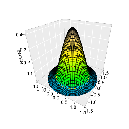
Figure 1: The radial ground state and the probability density for $V_{0}=2.1$. The circle on the polar plot indicates the well boundary $r=1$. The conspicuous tails depict qualitatively the tunelling effect.

Simulation data allow us to deduce an approximate form of the eigenfunction, see e.g. Fig. 1. As a byproduct of simulations we have computed the ratio of probabilities: that of localizing the state within the well area $P_{in}$, and that referring to the delocalized tail (beyond the well) $P_{out}$: .

$$\frac{P_{out}}{P_{in}}=\frac{\int\limits_{1}^{a}r^{2}\psi^{2}(r)dr}{\int\limits_{0}^{1}r^{2}\psi^{2}(r)dr}=\frac{1-4\pi\int\limits_{0}^{1}r^{2}\psi^{2}(r)dr}{4\pi\int\limits_{0}^{1}r^{2}\psi^{2}(r)dr}.$$ (16)

A concrete numerical outcome depends on $a$, but appears to stabilize for large values of $a$. In particular, for $V_{0}=2.1$ and $a=500$ we arrive at the ratio value $0.438$ indicating a conspicuous strength of the tunneling effect.

III Existence thresholds for higher purely radial eigenfunctions.

We can extend the methodology of Section II to set existence thresholds for higher radial bound states in $3D$. However, before proceeding further with the ultrarelativistic case, let us recall known facts about the standard ($(-\Delta+V)f=Ef$) Schrödinger spectral problem for the finite well, Gr ; VO .

If energy is measured in units $\hbar^{2}/2m$, while any a priori chosen radius $R>0$ stands for the length unit, the dimensional no-ground-state-in existence criterion $\sqrt{\frac{2mV_{0}R^{2}}{\hbar^{2}}}<\frac{\pi}{2}$ takes the form $V_{0}<\pi^{2}/4\sim 2.45$. We have exactly $n\geq 1$ bound states if the well potential obeys inequalities $(2n-1)^{2}\frac{\pi^{2}}{4}<V_{0}<(2n+1)^{2}\frac{\pi^{2}}{4}$. The corresponding eigenvalues are accessible by means of numerical methods only. W note a conspicuous (albeit rough) $n^{2}$ scaling of consecutive threshold values for $V_{0}$.

The situation is different in the ultrarelativistic case, where the analogous scaling is approximately linear in $n$, see e.g. stef ; kwasnicki0 for the related $1D$ discussion as well as for that on limits of its $3D$ validity, ZG1 .

In view of the previously established $1D$-$3D$ spectral link, if we are interested in the existence of the second and third $3D$ finite well eigenvalue, actually we need to deduce the existence threshold $V_{0}$ (we keep the $0.1$ accuracy limitation) for the $4$th and $6$th $1D$ well eigenvalues. This we have done numerically with $a=50$. Computation outcomes are collected in table II, where the notation $E_{(k,0)}$ with $k=1,2,...$ explicitly introduces the $l=0$ orbital label, ZG1 . The pertinent eigenfunctions are purely radial.

a	$E_{(1,0)}$ ($V_{0}=2.1$)	$E_{(2,0)}$ ($V_{0}=5.2$)	$E_{(3,0)}$ ($V_{0}=8.3$)
50	2.02603	5.13346	8.26733
$\infty$	2.03882	5.14626	8.28013

Table 2: $3D$ spherical well: approximate $V_{0}$ threshold values for the existence of (i) the ground state, (ii) first and (iii) second excited (purely radial) eigenstates (first three eigenvalues in the $l=0$ series). The cumulative correction of Remark 5, taking $E_{50}$ into $E_{\infty}$, equals $0.0128$.

For each of the considered threshold values, a lowering of a given $V_{0}$ value by $0.1$ is sufficient for the pertinent bound state (i)-(iii) in Table II not to exist. Some caution is necessary in connection with our explicit threshold values $V_{0}$. The $(-a,a)$ integrations are carried out numerically upon a definite partition unit choice (we have set the partition finesse at 0.001, c.f. Remark 4). Further tuning of the partition finesse would increase an integration accuracy and then a residual modification of $5.2$ or $8.3$ threshold values might in principle be necessary on the level of not displayed decimal digits.

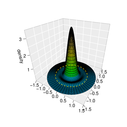
Figure 2: Second (first excited) radial eigenfunction in the $3D$ well, together with the polar plot for the related probability density, for $V_{0}=5.2$ and $a=50$.

The related eigenfunction has one nodal set (circle) and quickly decays (drops down) beyond the well area. We add that for $V_{0}=5.2$ the ground state energy ($a=50$) reads $2.38033$, to be set against the excited radial state eigenvalue $5.13346$.

The third radial bound state in the $3D$ well does exist for $V_{0}=8.3$ and has two disjoint nodal sets (circles).

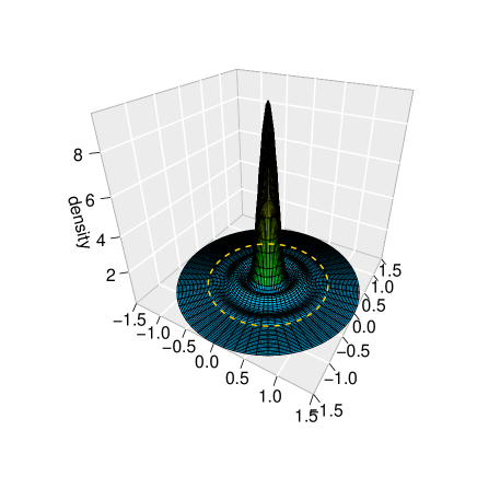
Figure 3: Third radial eigenfunction and the inferred probability density plot for $V_{0}=8.3$ and $a=50$. The circle on the polar plot indicates the well boundary $r=1$.

On the basis of data presented in Table II we realize that consecutive bound states are allowed to appear if $V_{0}$ changes approximately by $\pi$ (actually, we get $\sim 3.1$). It is consistent with the above mentioned linear scaling of threshold values, whose sharper version has been established for the $1D$ infinite ultrarelativistic well, kwasnicki0 . Indeed, in $1D$ there holds (which is a fairly good estimate beginning from $n=5$):

$$E_{n}=\frac{n\pi}{2}-\frac{\pi}{8}+\mathcal{O}\left(\frac{1}{n}\right),$$ (17)

so that $E_{2n+2}-E_{2n}\sim\pi$. Since for radial $3D$ bound states the $1D$ eigenvalue $E_{2n}$ actually coincides with the $n$th $3D$ eigenvalue.

IV Existence thresholds for orbitally nontrivial ($l>0$) eigenfunctions.

IV.1 $l=1$ eigenfunctions

In our study ZG1 of the infinite spherical well spectral problem, in addition to purely radial eigenfunctions, we have identified eigenfunctions that are not purely radial and thence belong to orbital sectors labeled by $l\geq 1$. These observations provide a useful guidance in case of the finite spherical well. Our further analysis will in part rely on the analytic approach to the evaluation of (singular) integrals, c.f. sections IV.A and B in Ref. ZG1 . Albeit the ultimate simulation algorithm will be entirely different from that employed in ZG1 . By integrating out all angular contributions, we arrive at purely radial integrals. The numerically-assisted (approximate) solution of the eigenvalue problem, can be addressed by means of the so-called Strang splitting method, succesfully used in $1D$ considerations of Ref. ZG2 . Its outline has been given in Section II.

In Ref. ZG1 we have shown that the ultrarelativistic infinite well eigenfunctions have a generic form $\psi_{(k,l,m)}(r,\theta,\phi)=f_{k}(r)Y_{l,m}(\theta,\phi)$, where $Y_{l,m}(\theta,\phi)$ are spherical harmonics in $\mathbb{R}^{3}$ and $k=1,2,...$ labels are uncorrelated with the $l=0,1.2,...$ orbital labels, while $|m|\leq l$ for each $l$. In the pertinent infinite well regime, we have imposed specific requirements concerning the functional form of $f_{k}(r)$. None of them is in use presently, in the finite well setting. Therefore, we shall employ another computation method (Strang splitting instead of Mathematica routines) than that of Ref. ZG2 , while leaving intact the factorization ansatz $\psi(r,\theta,\phi)=f(r)\,Y(\theta,\phi)$.

Let $\textbf{p}=(x_{1},x_{2},x_{3})\in\mathbb{R}^{3}$. Anticipating the $l=1$ ultimate eigensolution we first look for an eigenfunction in the functional form $\psi(\textbf{p})=x_{3}f(p)$, where $p=\sqrt{x_{1}^{2}+x_{2}^{2}+x_{3}^{2}}$ and $x_{3}=r\cos\theta\neq 0$. The purely radial function $f(p)$ is at the moment unknown and should follow from the eigenvalue equation

$$A\psi(\textbf{p})+V(\textbf{p})\psi(\textbf{p})=(I_{1}-I_{2})\psi(\textbf{p})+V(\textbf{p})\psi(\textbf{p})=E\psi(\textbf{p}).$$ (18)

The integral operator $A$ is here re-defined as a $(p.v.)$ computable difference of singular integrals $(I_{1}-I_{2})\psi(\textbf{p})$, where

$$A\psi(\textbf{p})={\frac{1}{\pi^{2}}}\left(\int\limits_{\mathbb{R}^{3}}{\frac{\psi(\textbf{p})du}{(\bf{u}-\bf{p})^{4}}}-\int\limits_{\mathbb{R}^{3}}{\frac{\psi(\textbf{u})du}{(\bf{u}-\bf{p})^{4}}}\right),$$ (19)

and $\textbf{u}=(u_{1},u_{2},u_{3})$ and $du$ indicates a three-dimensional integration.

In Ref. ZG1 we have described how to reduce $\mathbb{R}$ integrals, involved in (18) via (1), to the purely radial integration. C.f. Section IV.A, Eqs. (27)-(36) there in. We have constructed a rotation matrix $S$ in $\mathbb{R}^{3}$ such that

$$u_{i}=s_{i1}v_{1}+s_{i2}v_{2}+s_{i3}v_{3},\qquad i=1,2,3,$$ (20)

where $s_{ij}$ are matrix elements of $S$ such that

$$\sqrt{u_{1}^{2}+u_{2}^{2}+u_{3}^{2}}\xrightarrow{S}\sqrt{v_{1}^{2}+v_{2}^{2}+v_{3}^{2}}=r,$$ (21)

$$(u_{1}-x_{1})^{2}+(u_{2}-x_{2})^{2}+(u_{3}-x_{3})^{2}\xrightarrow{S}v_{1}^{2}+v_{2}^{2}+(v_{3}-\sqrt{x_{1}^{2}+x_{2}^{2}+x_{3}^{2}})^{2}.$$ (22)

We denote $\textbf{r}=(v_{1},v_{2},v_{3})$ and $|\textbf{v}|=r$.

Keeping in mind that both $I_{1}$ and $I_{2}$ are singular integrals and that the it is the $(p.v.)(I_{1}-I_{2})$ recipe that removes the involved all obstacles, we shall evaluate the integral entries separately, while passing to spherical coordinates with:

$$\begin{split}I_{1}(\bf{p})&=\frac{1}{\pi^{2}}\int\limits_{\mathbb{R}^{3}}\frac{x_{3}f(p)du}{((u_{1}-x_{1})^{2}+(u_{2}-x_{2})^{2}+(u_{3}-x_{3})^{2})^{2}}=\frac{x_{3}f(p)}{\pi^{2}}\int\limits_{\mathbb{R}^{3}}\frac{dv}{(v_{1}^{2}+v_{2}^{2}+(v_{3}-p)^{2})^{2}}\\ &=\frac{x_{3}f(p)}{\pi^{2}}\int\limits_{0}^{\infty}dr\int\limits_{0}^{2\pi}d\phi\int\limits_{0}^{\pi}d\theta\frac{r^{2}\sin\theta}{(r^{2}+p^{2}-2rp\cos\theta)^{2}}=\frac{x_{3}f(p)}{\pi p}\int\limits_{0}^{\infty}r\left(\frac{1}{(r-p)^{2}}-\frac{1}{(r+p)^{2}}\right)dr,\end{split}$$ (23)

and

$$\begin{split}I_{2}(\bf{p})&=\frac{1}{\pi^{2}}\int\limits_{\mathbb{R}^{3}}\frac{u_{3}f(u)d^{3}u}{((u_{1}-x_{1})^{2}+(u_{2}-x_{2})^{2}+(u_{3}-x_{3})^{2})^{2}}=\frac{s_{33}}{\pi^{2}}\int\limits_{0}^{\infty}dr\int\limits_{0}^{2\pi}d\phi\int\limits_{0}^{\pi}d\theta\frac{r^{3}f(r)\sin\theta\cos\theta}{(r^{2}+p^{2}-2rp\cos\theta)^{2}}\\ &=\frac{s_{33}}{2\pi p^{2}}(I_{21}+I_{22})=\frac{x_{3}}{2\pi p^{3}}(I_{21}+I_{22})\end{split}$$ (24)

where

$$\begin{split}I_{21}(p)&=\int\limits_{0}^{\infty}r(r^{2}+p^{2})f(r)\left(\frac{1}{(r-p)^{2}}-\frac{1}{(r+p)^{2}}\right)dr,\\ I_{22}(p)&=\int\limits_{0}^{\infty}rf(r)\left(\ln(r-p)^{2}-\ln(r+p)^{2}\right)dr.\end{split}$$ (25)

Accordingly, the $x_{3}\neq 0$ factor becomes irrelevant and we reduce Eq. (19) to the form:

$$(Af)(p)+V(p)f(p)=Ef(p)$$ (26)

where $(Af)(p)$ is a purely radial integral

$$(Af)(p)=\frac{1}{2\pi}\int\limits_{0}^{\infty}\left[\frac{r}{p}\left(2f(p)-\frac{r^{2}+p^{2}}{p^{2}}f(r)\right)\left(\frac{1}{(r-p)^{2}}-\frac{1}{(r+p)^{2}}\right)-\frac{rf(r)}{p^{3}}\left(\ln(r-p)^{2}-\ln(r+p)^{2}\right)\right]dr.$$ (27)

It is the eigenvalue problem with respect to $f(p)$ and $E$ which we shall address by means of the Strang method of Ref. ZG2 . One needs to remember about the $L^{2}$ scalar product and norm input in the Strang method. The scalar product $<f_{1}|f_{2}>$ we directly infer from $<\psi_{1}|\psi_{2}>$ (remembering that $\psi=x_{3}\,f$):

$$\int\limits_{0}^{\infty}dr\int\limits_{0}^{2\pi}d\phi\int\limits_{0}^{\pi}d\theta(r^{2}\sin\theta)(r\cos\theta f_{1}(r))(r\cos\theta f_{2}(r))=\frac{4\pi}{3}\int\limits_{0}^{\infty}r^{4}f_{1}(r)f_{2}(r)dr.$$ (28)

Consequently, the normalization coefficient is given by:

$$C^{2}\int\limits_{0}^{\infty}dr\int\limits_{0}^{2\pi}d\phi\int\limits_{0}^{\pi}d\theta r^{2}\sin\theta(r\cos\theta f(r))^{2}=\frac{4\pi C^{2}}{3}\int\limits_{0}^{\infty}r^{4}f^{2}(r)dr=1.$$ (29)

Eigenvalue problems of the type (26) and (27) have never been studied in the literature. Previously, ZG1 we have addressed that issue for the infinite spherical well. Now the considered spherical well is not merely finite, but shallow.

The Strang method has been adopted to solve (approximately) the pertinent eigenvalue problem in the orbital $l=1$ sector, c.f. for comparison our infinite well data of Ref. ZG1 . We stress that computation outcomes rely both on the choice of then integration boundary $a>0$ and the partition finesse, which we have set at the value $\Delta x=0.001$.

We have identified the existence of the orbital eigenstate in the $V_{0}=3.5$ well. We have also verified that for $V_{0}=3.4$ there is no $l=1$ eigenfunction.

a	E ($V_{0}=3.5$)
50	3.43477
100	3.44755
200	3.45393
500	3.45776
$\infty$	3.46036

Table 3: The first (and the only) orbital ($l=1$) eigenvalue for $V_{0}=3.5$: the $a$-dependence.

We point out that spacings between eigenvalues obtained for different choices of $a$ stay in a conspicuous agreement with our discussion in Section II. These are respectively $0.01278,0.00638,0.00383$ and roughly coincide with doubled values reported in Remark 5. We recall that the pertinent discussion has elucidated properties of the $1D$ integrations within the interval $[-a,a]$. In $3D$ we integrate with respect to the radial variable $r$, on the interval $[0,a]$.

The above observation allows in principle to interpolate results obtained for a given value of $a$ towards $\infty$, e.g. the $a=500$ eigenvalue might in principle be additively renormalized by $2\cdot 0.0013$. Such ”corrected eigenvalue would read $E_{(1,1)}^{(V_{0}=3.5)}=3.46036<3.5$ and is actually listed in Table III.

In the computation process for $V_{0}=3.5$, we recover the data necessary to depict the radial part of the eigenfunction $\psi_{(1,1,0)}$, (that is simply $rf(r)$) and the plots of related probability densities $|\psi_{(1,1,0)}(r,\theta,\phi)|^{2}$ and $|\psi_{(1,1,\pm 1)}(r,\theta,\phi)|^{2}$. We remind that the probability densities are $\phi$-independent and polar plots give an accurate visualization of the spatial properties of eigenfunctions.

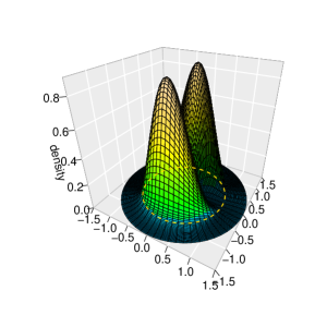
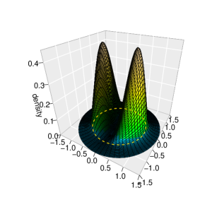
Figure 4: $V_{0}=3.5$: the radial section of $\psi_{(1,1,0)}$ and probability density plots for $|\psi_{(1,1,0)}(r,\theta,\phi)|^{2}$, $|\psi_{(1,1,\pm 1)}(r,\theta,\phi)|^{2}$. We point out that $|Y_{(l,m)}|$ is $\phi$-independent.

Quite analogously, we can demonstrate that, if $x_{3}f(p)$ is an eigenfunction with the eigenvalue $E_{(1,1)}^{(V_{0}=3.5)}=3.46036<3.5$, then $x_{1}f(p)$ and $x_{2}f(p)$ share with $x_{3}f(p)$ the same $f(p)$, being likewise the $E_{(1,1)}^{(V_{0}=3.5)}$ eigenfunctions. The eigenvalue is triply degenerate. Following the observations of Ref. ZG1 we expect that it is possible express the finite well eigenfunctions in terms of spherical harmonics. Indeed, Gr , we have $\psi_{(1,1,\pm 1)}(\textbf{x})=(x_{1}\pm ix_{2})f(p)=Y_{1,\pm 1}$ and $\psi_{(1,1,0)}=x_{3}f(p)=Y_{(1,0)}f(p)$.

The eigenvalue problem (26) admits other solutions, that can be retrieved by means of the Strang algorithm. We are interested in fairly shallow wells, hence it suffices to mention the next (excited orbital level) $l=1$ eigenfunction. It exists for $V_{0}=6.7$, while for $V_{0}=6.6$ we have proved the non-existence of eigenfunctions in the form $x_{3}f(p)$. The $V_{0}=6.7$ eigenvalue has an approximate value $6.61546$, obtained for $a=50$ and $\Delta x=0.001$. Its $a\to\infty$ interpolation (c.f. remark 5) equals $(6.61546+2\cdot(0.0064+0.0032+0.0019+0.0013))=6.64106<6.7$.

a	$E_{(1,1)}$ ($V_{0}=3.5$)	$E_{(2,1)}$ ($V_{0}=6.7$)
50	3.43477	6.61546
$\infty$	3.46036	6.64106

Table 4: First two eigenvalues in the $l=1$ series are admissible once the threshold value reaches $V_{0}=6.7$.

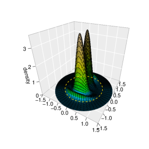
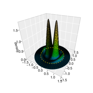
Figure 5: The radial section of $\psi_{(2,1,0)}$ and polar plots of probability densities $|\psi_{(2,1,0)}(r,\theta,\phi)|^{2}$, $|\psi_{(2,1,\pm 1)}(r,\theta,\phi)|^{2}$ for $V_{0}=6.7$.

IV.2 $l=2$ eigenfunctions

With the increase of the well depth (or height) above $V_{0}=3.5$ the $l=2$ orbital eigenfunctions are allowed to appear. We shall now pass to $l=2$ proper, while presuming the factorization $\psi_{(k,l,m)}(r,\theta,\phi)=f_{k}(r)Y_{l,m}(\theta,\phi)$ of eigenfunctions.

We shall demonstrate that $\psi_{1,2,0}(\textbf{x})=(3x_{3}^{2}-p^{2})f(p)$, with $p=\sqrt{x_{1}^{2}+x_{2}^{2}+x_{3}^{2}}$, $p\neq 0$ actually is an orbital solution of Eq. (18). Integrations are carried out in a fashion similar to that corresponding to the case $l=1$. The expression $A\psi(\bf{p})$ is decomposed into (remember about the $(p.v.)$ recipe) the difference $I_{1}-I_{2}$, where

$$\begin{split}I_{1}(p)&=\frac{1}{\pi^{2}}\int\limits_{\mathbb{R}^{3}}\frac{(3x_{3}^{2}-p^{2})f(p)d^{3}u}{((u_{1}-x_{1})^{2}+(u_{2}-x_{2})^{2}+(u_{3}-x_{3})^{2})^{2}}=\frac{(3x_{3}^{2}-p^{2})f(p)}{\pi^{2}}\int\limits_{\mathbb{R}^{3}}\frac{d^{3}v}{(v_{1}^{2}+v_{2}^{2}+(v_{3}-p)^{2})^{2}}\\ &=\frac{(3x_{3}^{2}-p^{2})f(p)}{\pi^{2}}\int\limits_{0}^{\infty}dr\int\limits_{0}^{2\pi}d\phi\int\limits_{0}^{\pi}d\theta\frac{r^{2}\sin\theta}{(r^{2}+p^{2}-2rp\cos\theta)^{2}}=\frac{(3x_{3}^{2}-p^{2})f(p)}{\pi p}\int\limits_{0}^{\infty}r\left(\frac{1}{(r-p)^{2}}-\frac{1}{(r+p)^{2}}\right)dr,\end{split}$$ (30)

and

$$I_{2}(p)=\frac{1}{\pi^{2}}\int\limits_{\mathbb{R}^{3}}\frac{(3u_{3}^{2}-u^{2})f(u)d^{3}u}{((u_{1}-x_{1})^{2}+(u_{2}-x_{2})^{2}+(u_{3}-x_{3})^{2})^{2}}=\frac{1}{\pi^{2}}\int\limits_{\mathbb{R}^{3}}\frac{[3(s_{11}v_{1}+s_{12}v_{2}+s_{13}v_{3})^{2}-v^{2}]f(v)d^{3}v}{(v_{1}^{2}+v_{2}^{2}+(v_{3}-p)^{2})^{2}}.$$ (31)

$I_{2}(p)$ may be given a form of the sum $I_{2}=I_{21}+I_{22}+I_{23}+I_{24}$, where

$$\begin{split}I_{21}&=\frac{3s_{11}^{2}}{\pi^{2}}\int\limits_{\mathbb{R}^{3}}\frac{v_{1}^{2}f(v)d^{3}v}{(v_{1}^{2}+v_{2}^{2}+(v_{3}-p)^{2})^{2}}=\frac{3s_{11}^{2}}{\pi^{2}}\int\limits_{0}^{\infty}dr\int\limits_{0}^{2\pi}d\phi\int\limits_{0}^{\pi}d\theta\frac{r^{2}\sin\theta(r\cos\phi\sin\theta)^{2}f(r)}{(r^{2}+p^{2}-2rp\cos\theta)^{2}}\\ &=\frac{3s_{11}^{2}}{\pi}\int\limits_{0}^{\infty}\left[-\frac{r^{2}}{p^{2}}-\frac{r(r^{2}+p^{2})}{4p^{3}}\left(\ln(r-p)^{2}-\ln(r+p)^{2}\right)\right]f(r)dr,\end{split}$$ (32)

$$\begin{split}I_{22}&=\frac{3s_{12}^{2}}{\pi^{2}}\int\limits_{\mathbb{R}^{3}}\frac{v_{2}^{2}f(v)d^{3}v}{(v_{1}^{2}+v_{2}^{2}+(v_{3}-p)^{2})^{2}}=\frac{3s_{12}^{2}}{\pi}\int\limits_{0}^{\infty}\left[-\frac{r^{2}}{p^{2}}-\frac{r(r^{2}+p^{2})}{4p^{3}}\left(\ln(r-p)^{2}-\ln(r+p)^{2}\right)\right]f(r)dr,\end{split}$$ (33)

$$\begin{split}I_{23}&=\frac{3s_{13}^{2}}{\pi^{2}}\int\limits_{\mathbb{R}^{3}}\frac{v_{3}^{2}f(v)d^{3}v}{(v_{1}^{2}+v_{2}^{2}+(v_{3}-p)^{2})^{2}}\\ &=\frac{3s_{13}^{2}}{2\pi p^{3}}\int\limits_{0}^{\infty}\left[r(r^{4}+p^{4})\left(\frac{1}{(r-p)^{2}}-\frac{1}{(r+p)^{2}}\right)+r(r^{2}+p^{2})\left(\ln(r-p)^{2}-\ln(r+p)^{2}\right)\right]f(r)dr,\end{split}$$ (34)

$$\begin{split}I_{24}&=-\frac{1}{\pi^{2}}\int\limits_{\mathbb{R}^{3}}\frac{v^{2}f(v)d^{3}v}{(v_{1}^{2}+v_{2}^{2}+(v_{3}-p)^{2})^{2}}=-\frac{1}{\pi p}\int\limits_{0}^{\infty}r^{3}f(r)\left(\frac{1}{(r-p)^{2}}-\frac{1}{(r+p)^{2}}\right)dr.\end{split}$$ (35)

We deal with singular integrals hence the $I=(p.v.)(I_{1}-I_{2})$ recipe must be kept in mind. Collecting all terms together we arrive at $I(p)=(3x_{3}^{2}-p^{2})(Af)(p)$, where $(Af)(p)$ of Eq. (26) has the $(p.v.)$ form

$$(Af)(p)=$$ (36)

$$\frac{1}{4\pi}\int\limits_{0}^{\infty}\left[\frac{r}{p}\left(4f(p)-f(r)\frac{3(r^{4}+p^{4})-2r^{2}p^{2}}{p^{4}}\right)\left(\frac{1}{(r-p)^{2}}-\frac{1}{(r+p)^{2}}\right)-3f(r)\frac{r(r^{2}+p^{2})}{p^{5}}\left(\ln(r-p)^{2}-\ln(r+p)^{2}\right)\right]dr.$$

Like in case of $l=1$ where the factor $x_{3}$ has been spurious, we identify $(3x_{3}^{2}-p^{2})\neq 0$ as the spurious factor, thus reducing the eigenvalue problem to the form (26). The Strang algorithm is employed again, with the assumption about the normalization of $\psi$

$$C^{2}\int\limits_{0}^{\infty}dr\int\limits_{0}^{2\pi}d\phi\int\limits_{0}^{\pi}d\theta r^{2}\sin\theta(3r^{2}\cos^{2}\theta-r^{2})^{2}f^{2}(r)=\frac{16\pi C^{2}}{5}\int\limits_{0}^{\infty}r^{6}f(r)dr=1,$$ (37)

and the scalar product $<f_{1}|f_{2}>$ directly inferred from $<\psi_{1}|\psi_{2}>$, under an assumption that $\psi=(3x_{3}^{2}-p^{2})f(p)$:

$$\int\limits_{0}^{\infty}dr\int\limits_{0}^{2\pi}d\phi\int\limits_{0}^{\pi}d\theta r^{2}\sin\theta(3r^{2}\cos^{2}\theta-r^{2})^{2}f_{1}(r)f_{2}(r)=\frac{16\pi}{5}\int\limits_{0}^{\infty}r^{6}f_{1}(r)f_{2}(r)dr.$$ (38)

We have no clues about the threshold $V_{0}$ value above which the first $l=2$ eigenstate does appear. Our reasoning was somewhat empirical (e.g. via numerical guesses and tests). With $a=50$ we have found the for $V_{0}=4.8$ the orbital $l=2$ eigenstate exists, while for $V_{0}=4.7$ there is none.

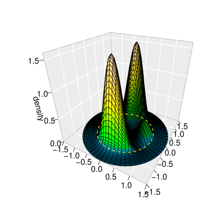
Figure 6: $V_{0}=4.8$: the radial section of $\psi_{(1,2,0)}$ and polar plots for the probability density $|\psi_{(1,2,0)}(r,\theta,\phi)|^{2}$.

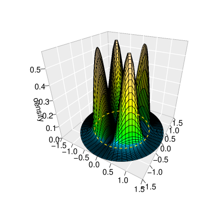
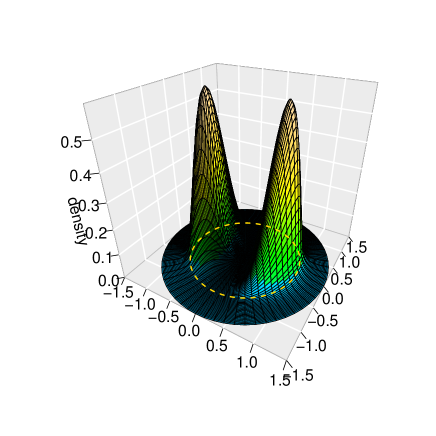
Figure 7: Polar plots of probability densities $|\psi_{(1,2,\pm 1)}(r,\phi,\theta)|^{2}$ and $|\psi_{(1,2,\pm 2)}(r,\phi,\theta)|^{2}$ for $V_{0}=4.8$.

a	E ($V_{0}=4.8$)
50	4.74184
100	4.75463
200	4.76102
500	4.76486
$\infty$	4.76746

Table 5: $V_{0}=4.8$: the $a$-dependence of the radial eigenvalue $E_{(1,2)}$.

We can evaluate the energy intervals (gaps) between consecutive $a$-dependent eigenvalues. They read $0.01279,0.00639,0.00384$ and are roughly (up to the last decimal digit) doubled $1D$ gaps of Remark 5. Accordingly, we anticipate the $a\to\infty$ eigenvalue by taking $E(a=500)$ and renormalizing it (additively) by $2\cdot 0.0013$. That implies $E_{(1,2)}^{V_{0}=4.8}=4.76746$.

One can verify that functions of the form

$$(x_{1}^{2}-x_{2}^{2})f(p),\quad x_{1}x_{2}f(p),\quad x_{1}x_{3}f(p),\quad x_{2}x_{3}f(p),$$ (39)

are eigenfunctions corresponding to the common with $\psi_{1,2,0}(\textbf{x})=(3x_{3}^{2}-p^{2})f(p)$ eigenvalue $E_{(1,2)}$ of Table V. An equivalent eigenfunction set displays a manifest dependence on spherical harmonics, in consistency with the infinite well observations of Ref. ZG1 :

$$\begin{split}\psi_{(1,2,0)}(p)&=C(3x_{3}^{2}-p^{2})f(p)=\tilde{C}p^{2}Y_{2}^{0}f(p),\\ \psi_{(1,2,\pm 1)}(p)&=Cx_{3}(x_{1}\pm ix_{2})f(p)=\tilde{C}p^{2}Y_{2}^{\pm 1}f(p),\\ \psi_{(1,2,\pm 2)}(p)&=C(x_{1}\pm ix_{2})^{2}f(p)=\tilde{C}p^{2}Y_{2}^{\pm 2}f(p).\end{split}$$ (40)

By collecting together the obtained spectral data, we can tabulate the threshold well height (depth) values $V_{0}$ so that the maximal number of bound states can be clearly identified. To this end we provide a cumulative table (Table VI) of computed eigenvalues for $2.1\leq V_{0}\leq 8.3$, comprising all $0\leq l\leq 2$ entries. We keep intact the presumed $0.1$ inaccuracy with which a given existence threshold is located, i.e. given the depicted $V_{0}$ value, the actual threshold is located within the interval $(V_{0}-0.1,V_{0}]$.

$V_{0}$	2.1	3.5	4.8	5.2	6.7	8.1	8.3	$\ldots$	$\infty$
$l=0$	2.03882	2.27399	2.37186	2.39313	2.45288	2.49118	2.49575	…	$2.754769=E_{(1,0)}$
	-	-	-	5.14626	5.31977	5.40211	5.41186	…	$5.892214=E_{(2,0)}$
	-	-	-	-	-	-	8.28013	…	$9.033009=E_{(3,0)}$
$l=1$	-	3.46036	3.60459	3.63433	3.71631	3.76785	3.77396	…	$4.121332=E_{(1,1)}$
	-	-	-	-	6.64106	6.75640	6.76877	…	$7.342181=E_{(2,1)}$
$l=2$	-	-	4.76746	4.80535	4.90712	4.96999	4.97740	…	$5.400079=E_{(1,2)}$
	-	-	-	-	-	8.04169	8.05689	…	$8.718436=E_{(2,2)}$

Table 6: Computed eigenvalues (interpolated in accordance with the $a\to\infty$ recipe of Remark 5) for various $V_{0}$ choices. The last column, reproducing the corresponding infinite spherical well eigenvalues $E_{k,l)}$, has been borrowed from Table III in Ref. ZG1 .

In Table VI, we can read out a maximal number of admitted $l\leq 2$ eigenvalues, together with an order according to which the consecutive eigenvalues are allowed to appear with the growth of $V_{0}$.

We indicate that $E_{(1,3)}=6.630371$, ZG1 , hence one can expect an emergence of the first $l=3$ eigenvalue in the finite well at $V_{0}$ around $5.7-5.9$. In view of $E_{(2,3)}=10.045716$, in the finite well the second $l=3$ eigenvalue could possibly appear for $V_{0}$ about $9.2-9.3$. Accordingly, Table VI up to $V_{0}=5.2$ depicts a maximal number of admitted eigenvalues, while for $6.7\leq V_{0}\leq 8.3$ only a single (actually the first) $l=3$ explicit eigenvalue is missing in the Table.

V Outlook

We recall that the basic goal of Ref. gar0 was to set on solid grounds the quantization programme which completely avoids any reference to a classical mechanics of massive particles, traditionally viewed as a conceptual support for the choice of the Hamiltonian operator within the standard Schrödinger wave mechanics. We have indicated there that a commonly adopted form of the Hamiltonian (minus Laplacian plus a perturbing potential) an exception rather than a universally valid feature of an admissible quantum theory, for which the choice of $-(\Delta)^{\alpha/2}$, $\alpha\in(0,2)$, instead of $-\Delta$ does not at all exhaust an infinity of other candidate operators (c.f. the Lévy-Khintchine formula, gar0 ) .

In the present paper our focus was on spectral properties of the bound states in the ultrarelativistic case. That amounts to a concrete choice of $\alpha=1$, resulting in the Cauchy operator $\sqrt{-\Delta}$. It is perhaps the only directly physics-motivated example, which can be singled out from the one-parameter family of Lévy stable operators $(-\Delta)^{\alpha/2}$. Each of these operators gives rise to a family of related Schrödinger-type spectral problems, see e.g. carmona .

The absence of any natural mass parameter is a conspicuous feature of Lévy-Schrödinger spectral problems and their ultrarelativistic (Cauchy) version in particular.

There are few only spectral solutions that have been obtained in the ultrarelativistic regime, with the main activity arena being $1D$. In particular, the $1D$ Cauchy oscillator problems has been analytically solved in Refs. gar ; lorinczi2 . Its anharmonic version has been addressed in ref. lorinczi3 . The $3D$ Cauchy oscillator has been addressed in remb in the $l=0$ sector, hence with no orbitally nontrivial outcomes.

We have contributed to an active research on Cauchy operators with exterior Dirichlet boundary data in $1D$ (infnite well problem), extending that analysis to the finite well spectral problem, ZG2 ; ZG3 , see also duo ; dyda0 and GZ .

In the previous paper ZG1 , we have addressed the general $3D$ spectral problem for the ultrarelativistic spherical infinite well, see e.g. dyda0 ; dyda for related considerations. Presently our focus was on the more physically appealing case of the finite spherical well.

We have discussed, in part with the aid of numerical methods, the existence issue for the ground state. Next, approximate threshold values for the emergence of higher excited states were established, both in the radial and nontrivially orbital sectors. The corresponding eigenfunction shapes were established as well, while accounting for the degeneracy of the spectrum. The eigenvalues obtained under the shallow well premises were collected in the Table VI, and set in correspondence (albeit somewhat distant) with those for the infinite $3D$ well.

We end up with a potentially interesting research hint of Ref. ZG1 : ”quite an ambitious research goal could be an analysis a spatially random distribution (”gas”) of finite ultrarelativistic spherical wells, embedded in a spatially extended finite energy background”. This could be further source of inspirations in attempts towards understanding how (possibly on large spatial scales) the energy can be stored or accumulated in the form of bound states of Schrödinger - type quantum systems, that are devoid of any mass.

Ackonwledgement: We would like to express our gratitude to Professor Jozsef Lőrinczi for illuminating exchanges on various aspects of finite well spectral problems for fractional Laplacians, c.f. thanks in the text.

References

- (1) K. Kaleta and J. J. Lőrinczi, Transition in the decay rates of stationary distributions of Lévy motion in an energy landscape, Phys. Rev. E 93, (2016), 022135.
- (2) E. V. Kirichenko, P. Garbaczewski, V. Stephanovich and M. Żaba, Lévy flights in an infnite potential well as a hypersingular Fredholm problem, Phys. Rev. E 93, (2016), 052110.
- (3) R. Weder, ”Spectral analysis of pseudodifferential operators, J. Funct. Anal. 20, 319, (1975)
- (4) Spectral theory of the operator , Commun. Math. Phys. 53, 285, (1977)
- (5) R. Carmona, Path integral for relativistic Schrödinger operators, in: ”Schrödinger Operators”, edited by H. Holden and A. Jensen, Lecture Notes in Physics 345, pp. 65-92, (Springer, NY, 1989)
- (6) R. Carmona, W. C. Masters and B. Simon, Relativistic Schrödinger operators: Asymptotic behavior of eigenfunctions, J. Funct. Anal. 91, 117, (1990)
- (7) E. H. Lieb and R. Seiringer, ”The Stability of Matter in Quantum Mechanics”, (Cambrdige University Press, 2009).
- (8) J. Lőrinczi, F. Hiroshima and V. Betz, ”Feynman-Kac-Type Theorems and Gibbs Measures on Path Space”, (De Gruyter, Berlin, 2011).
- (9) M. Żaba and P. Garbaczewski, Ultrarelativistic bound states in the spherical well, J. Math. Phys. 57, (2016) 072302.
- (10) M. Kwaśnicki, Ten equivalent definitions of the fractional Laplace operator, arXiv:1507.07356 [math.AP].
- (11) M. Kwaśnicki, Eigenvalues of the fractional Laplace operator in the interval, J. Funct. Anal. 262, 2379, (2012).
- (12) M. Żaba and P. Garbaczewski, Solving fractional Schrödinger-type spectral problems: Cauchy oscillator and Cauchy well, J. Math. Phys. 55, (2014) 092103.
- (13) M. Żaba and P. Garbaczewski, Nonlocally-induced (fractional) bound states: Shape analysis in the infinite Cauchy well, J. Math. Phys. 56, 123502, (2015).
- (14) Siwei Duo and Yanzhi Zhang, Computing the ground state and first excited states of the fractional Schrödinger equation in an infinite potential well, Commun. Comput. Phys. 18, 321, (2015).
- (15) B. Dyda, Fractional calculus for power functions and eigenvalues of the fractional laplacian, Fractional Calculus and Applied Analysis, 15, 4, 536-555, (2012).
- (16) B. Dyda, A. Kuznetsov and M. Kwa nicki, Eigenvalues of the fractional Laplace operator in the unit ball, arXiv:1509.08533 (2015).
- (17) P. Garbaczewski and Żaba, Nonocally induced (quasirelativistics) bound states: Harmonic confinemnt and the finite well, Acta Phys. Pol. B46, 949, (2015).
- (18) J. Lőrinczi, private communication.
- (19) K. Kaleta and J. Lőrinczi, Fall-off of eigenfunctions for non-local Schrödinger operators with decaying potentials, arXiv:1503.03508.
- (20) F. Hiroshima and J. Lőrinczi, Lieb-Thirring bound for Schrödinger operators with Bernstein functions of the Laplacian, Commun. on Stochastic Analysis, 6, 589, (2012)
- (21) D. J. Griffiths, Introduction to Quantum Mechanics, 2nd Edition, (2005).
- (22) J. W. Van Orden, Quantum Mechanics Lecture Notes, (2007), http://ww2.odu.edu/ skuhn/PHYS621/WvOquantum.pdf.
- (23) P. Garbaczewski and V. Stephanovich, L vy flights and nonlocal quantum dynamics, J. Math. Phys. 54, 072103, (2013).
- (24) P. Garbaczewski and V. Stephanovich, Lévy flights in inhomogeneous environments, Physica A 389, 4419, (2010).
- (25) J. Lőrinczi and J. Małecki, Spectral properties of the massless relativistic harmonic oscillator, J. Diff. Equations, 251, 2846, (2012).
- (26) K. Kowalski and J. Rembieliński, The relativistic massless harmonic oscillator, Phys. Rev. A81, 012118, (2010).
- (27) J. Lőrinczi, K. Kaleta and S. Durugo, Spectral and analytic properties of nonlocal Schrödinger operators and related jump processes, Comm. Apppl. Industrial Math. 6(2), e-534, (2015).