Stellar electron capture rates on neutron-rich nuclei and their impact on core-collapse

Abstract

During the late stages of gravitational core-collapse of massive stars, extreme isospin asymmetries are reached within the core. Due to the lack of microscopic calculations of electron capture (EC) rates for all relevant nuclei, in general simple analytic parameterizations are employed. We study here several extensions of these parameterizations, allowing for a temperature, electron density and isospin dependence as well as for odd-even effects. The latter extra degrees of freedom considerably improve the agreement with large scale microscopic rate calculations. We find, in particular, that the isospin dependence leads to a significant reduction of the global EC rates during core collapse with respect to fiducial results, where rates optimized on calculations of stable $fp$-shell nuclei are used. Our results indicate that systematic microscopic calculations and experimental measurements in the $N\approx 50$ neutron rich region are desirable for realistic simulations of the core-collapse.

I Introduction

Electron capture (EC) on nuclei plays a crucial role in high density astrophysical environments and determines many processes such as $r$-process nucleosynthesis Goriely15 , heating Gupta06 and cooling of the accreting neutron star crust Schatz14 , thermonuclear explosions of accreting white dwarfs and explosive nucleosynthesis Iwamoto99 ; Brachwitz00 , the late stage evolution of massive stars Aufderheide94 ; Heger2001 and core-collapse (CC) supernovae Hix2003 ; Janka2007 ; Langanke03 .

In particular, during late stage stellar evolution EC is responsible for a number of important phenomena. First, it reduces the pressure provided by the degenerate relativistic electron gas in order to balance gravitation. It also cools the core by producing neutrinos which, for mass densities smaller than about $10^{11}$ g/cm³ (which corresponds to baryon number densities, $n_{B}$, of about $6\cdot 10^{-5}$ fm^-3) leave the star unhindered. Finally, EC determines the star’s composition via the electron-to-baryon ratio $Y_{e}$, equal to the proton fraction $Y_{p}=n_{p}/n_{B}$ due to charge neutrality. $n_{p}$ denotes here the charge density.

In a previous paper Raduta16 we have shown that nuclear statistical equilibrium (NSE) averaged EC rates strongly depend, in the late stages of pre-bounce evolution of the central element of a collapsing star, on the experimentally unknown binding energies of nuclei far beyond the stability valley. By controlling the evolution of $N=82$ and $N=50$ shell gaps in neutron-rich nuclei, we have shown that nuclear abundances can be strongly modified. As a consequence, the average EC rate may increase up to 30%. This study already underlined the need of additional experimental measurements and/or microscopic calculations at the neutron-rich edge of the known isotopic table.

Total EC rates are not only influenced by the nuclear distribution, but by the rates on individual nuclei, too. This aspect was recently addressed in Ref. Sullivan16 . Core collapse simulations were performed, considering a huge variety of progenitor models and several different equations of state (EoS). Individual EC rates were thereby systematically scaled by factors ranging from 2 to 10 with respect to the fiducial values taken from Refs. LMP ; Langanke03 ; Oda and the analytic parameterization of Ref. Langanke03 . The mass of the inner core at bounce and the maximum of the neutrino luminosity peak were found to augment (diminish) by 16% (4%) and, respectively, 20% when the EC rates are scaled by a factor of 0.1 (10). Moreover, it was shown that the modification of EC rates affects much more strongly the bounce properties than the progenitor model or the EoS. The results of the simulations were found to be most sensitive to a possible reduction in the EC rates for neutron rich nuclei near the $N$ = 50 closed shell. This finding is very interesting for future experiments with exotic beams.

This pedagogical study has clearly shown how much the lack of reliable information on EC rates on the relevant neutron-rich nuclei can impact the dynamics of core collapse. However, a global modification of all EC rates by a common factor – the same for all nuclei and all thermodynamic conditions – is clearly not realistic. Therefore, awaiting for more detailed microscopic calculations, it is timely to try to understand the different physical effects entering the EC rates in order to better control them outside the region where calculations constrained by experimental data are available. To this aim, instead of arbitrarily varying individual rates as in Ref.Sullivan16 , we try here to obtain some hints on their physical behavior at high electron density, temperature and isospin ratio from the trends observed in the region covered by microscopic calculations. Specifically we extend the existing analytic parameterizations in several ways to incorporate different physical effects and improve the reliability of the extrapolation to regions not covered by microscopic calculations.

We shall show that these improved parameterizations can lead to a reduction of the average EC rate with respect to previous estimations. Over a certain density domain, the reduction factor is as high as one order of magnitude, which corresponds to the maximum reduction considered in Ref. Sullivan16 .

To illustrate our findings, we will consider here some typical thermodynamic conditions. They are taken from two different core collapse trajectories reported in Ref. Juodagalvis_2010 . They correspond to the pre-bounce evolution of the central element of the star with an enclosed mass of 0.05 solar masses, for two progenitors, a $15M_{\odot}$ and a $25M_{\odot}$ one Heger2001 ; Hix2003 . Similar to our previous work, see Ref. Raduta16 , the modified EC rates will be added perturbatively. This means that we neglect for this exploratory work the influence of the modified rates on the time evolution of baryon number density $n_{B}$, temperature $T$ and proton fraction $Y_{p}$ throughout the collapse. Consequently, our quantitative predictions contain some uncertainties, and we cannot exclude that a consistent use of improved EC rates in a full core collapse simulation would produce an effect different than the one shown in the present work. However, qualitatively, our results are robust and the observed effect is large enough such that we expect in any case that it will have non-negligible impact on the dynamics of the collapse.

Given the thermodynamical conditions, we evaluate the chemical composition of matter and in particular nuclear abundances via the extended NSE model of Ref. Gulminelli15 . Experimental nuclear masses Audi supplemented by predictions of the 10-parameter mass model of Duflo and Zuker DZ10 are used. EC rates are calculated based on an analytic parameterization proposed in Ref. Langanke03 , fitted on large scale shell model calculations of $fp$-shell nuclei LMP ; Langanke00 . Three refinements of the original parameterization will be proposed: The average Gamow-Teller (GT) transition energy $\Delta E$ will be first allowed to depend on temperature and electron density, second on isospin, and finally, on the odd-even character of individual nuclei. These latter dependencies are inspired by the isospin asymmetry and odd-even dependence of the GT₊-resonance, shown by both experimental data and theoretical calculations (see for instance Juodagalvis05 ; Langanke00 ; Batist10 ).

The paper is organized as follows. Information on the thermodynamic conditions of the considered core collapse trajectories and the corresponding matter composition are given in Section II. The different prescriptions for the calculation of EC rates are discussed in Section III. The resulting EC rates averaged over the nuclear distributions obtained from the NSE along the considered trajectories are presented in Section IV. In Section V we summarize the present work.

II Thermodynamic conditions and matter composition

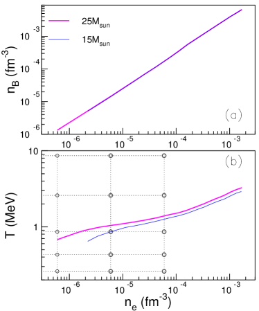
Figure 1: Thermodynamic conditions explored during collapse by the central elements of two progenitors, a $15M_{\odot}$ and $25M_{\odot}$ one, from Ref.Juodagalvis_2010 . Baryon number density (a) and temperature (b) are plotted as a function of the electron density $n_{e}$. The grid on panel (b) indicates the temperature-electron density grid of the tables for weak interaction rates from Ref. LMP .

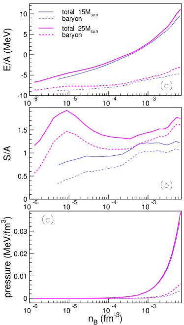
Figure 2: Results of the extended NSE model of Ref. Gulminelli15 using thermodynamic conditions reported in Ref. Juodagalvis_2010 of Fig. 1. Baryonic and total energy per baryon (a), entropy per baryon (b) and pressure (c) are plotted as a function of baryonic density.

The pre-bounce evolution of a collapsing star follows a complicated trajectory in the $T$, $n_{B}$ and $Y_{p}=Y_{e}$ space in response to different physical processes, including weak interactions. However, according to the theory of adiabatic collapse Goldreich , the central part of the core is expected to collapse homologously, meaning that the central densities and temperatures should manifest a more or less universal pattern taken as function of $Y_{e}$, as confirmed by detailed numerical simulations Yahil83 ; Bruenn85 ; Aufderheide94 .

In Fig. 1, we show the thermodynamic conditions at the center of the star during infall, resulting from two simulations Heger2001 ; Hix2003 with two different progenitors, a 15 $M_{\odot}$ and a 25 $M_{\odot}$ one. The central element within these spherically symmetric simulations corresponds to an enclosed mass of 0.05 $M_{\odot}$. Weak interactions rates have thereby been determined from a simple NSE matter composition together with rates taken from Refs. Langanke00 ; LMP , see Ref. Juodagalvis_2010 . On panel (b), the electron density-temperature grid of the weak interaction data base of Ref. LMP is represented as well. It is obvious that the highest electron densities reached during infall lie outside the grid domain and the temperatures, $T$, are situated in a region where the mesh is sparse.

Fig. 2 offers complementary information on the considered trajectories. It shows, as a function of the baryon number density, the baryonic and total energy per baryon (panel (a)), entropy per baryon (panel (b)) and pressure (panel (c)) as obtained within the extended NSE model of Ref. Gulminelli15 . We can see that the slight progenitor dependence exhibited by the temperature evolution (Fig. 1(b)) is somewhat amplified in other thermodynamic variables, notably the entropy per particle. This is due to the fact that these quantities strongly depend on the matter composition, which depends exponentially on temperature. Thus, even if the inner core evolves homologously, some progenitor dependence remains within the thermodynamic conditions and we will keep thus both trajectories for the discussion within this paper.

The matter composition along the two trajectories was investigated in detail in Ref. Raduta16 . It was shown in particular that the distributions of nuclei are broad at all times, and that individual nuclei become more neutron rich subsequently to the deleptonisation and decrease in $Y_{p}$ of the whole system. Nuclei with a mass number $A>20$ (called ”heavy” hereafter) bind an important amount of matter, even if their mass fraction decreases as the collapse advances and the temperature rises. In addition, if binding energies of nuclei are described by a model with strong shell gaps far from stability, as the DZ10 model DZ10 , the nuclear distributions are characterized by a competition between the $N=50$ and $N=82$ magic numbers Raduta16 .

III Electron capture rates

The first systematic study of weak interaction rates under stellar conditions is due to Fuller, Fowler and Newman. In a series of papers published in the ’80s, they pointed out the particular role played by the GT giant resonance for both electron capture and $\beta$-decays, and parameterized its contribution based on an independent particle model FFN80-82 ; FFN82 ; FFN85 . The resulting reaction rates for nuclei with mass numbers between 21 and 60, considered of chief importance in astrophysics, were made available in tabulated form FFN82 . Analytic parameterizations, where structure and phase space contributions are factorized, were proposed in Ref. FFN82 , too.

It is well known since these pioneering works that capture rates on heavy nuclei dominate the capture probability, though lighter nuclei cannot be neglected Raduta16 ; Fuller10 . This is due to the fact that the probability of capturing an electron is trivially hindered for large and negative reaction Q-value, defined as $Q(A,Z)=M(A,Z)-M(A,Z-1)+m_{e}$. $M(A,Z)$ denotes here the mass of a nucleus with $Z$ protons and $N=A-Z$ neutrons, and $m_{e}$ is the electron mass. The $Q$-value gives the relevant energy scale of the capture process at constant electron energy. Light nuclei, for which few stable isobars exist, have in general very low $Q$-values. For $fp$-shell nuclei around $A\approx 50$, the nuclear chart starts to widen and the $Q$-value increases.

Of course, lower $Q$-values might be compensated by higher abundances such that in an astrophysical situation still light nuclei may dominate. Therefore, we show in Fig. 3, the average $Q$-value, $\langle Q\rangle=\sum_{A,Z}n_{A,Z}Q(A,Z)/\sum_{A,Z}n_{A,Z}$, and average isospin asymmetry, $\langle I\rangle=\sum_{A,Z}n_{A,Z}(1-2Z/A)/\sum_{A,Z}n_{A,Z}$, throughout the CCSN trajectories of Ref. Juodagalvis_2010 . $n_{A,Z}$ represents the abundance per unit volume of the nucleus with $A$ nucleons and $Z$ protons. Nuclear abundances have been calculated within the extended NSE model of Ref. Gulminelli15 as detailed in the previous section. Light nuclei ($2\leq A<20$) are labeled by filled dots and heavy nuclei ($A\geq 20$) by open dots. The errors bars indicate the width of the nuclear distributions. It is obvious that for the considered thermodynamic conditions within the collapse phase of a CCSN, heavy nuclei systematically have larger average $Q$-values and, therefore, higher EC rates.

The widening of the region of nuclear stability also implies that higher values of the average isospin asymmetry can be reached for heavier nuclei. As expected from elementary considerations on nuclear stability, and clearly visible on Fig. 3, $\langle Q\rangle$ decreases with increasing neutron richness. Furthermore, due to the competition among $N$-magic numbers Raduta16 , wide distributions characterize heavy fragment production under all thermodynamic conditions. Contrary to heavy clusters whose properties vary strongly as the collapse proceeds, light clusters, defined on a quite limited mass domain and highly dominated by $\alpha$-particles, show an almost constant $\langle Q\rangle$-value and, in the late stages before bounce, a very large variation with isospin. The latter effect arises from the increasing contribution of loosely bound nuclei with $Z>2$ and large isospin, allowed by high temperatures and densities and low $Y_{p}=Y_{e}$ values, met in the late stage of the collapse.

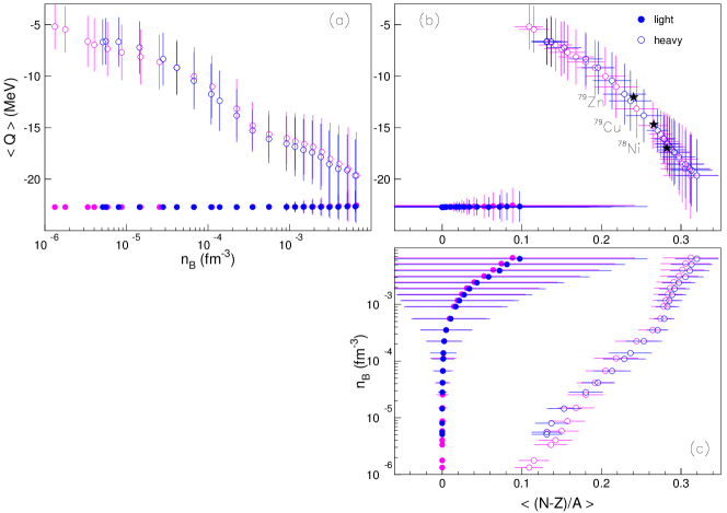
Figure 3: Average electron-capture $\langle Q\rangle$-value as a function of baryon number density for heavy ($A\geq 20$) and light ($2\leq A<20$) clusters (a), the same versus average isospin asymmetry $\langle(N-Z)/A\rangle$ (b) and $\langle(N-Z)/A\rangle$ versus baryon number density (c). The thermodynamic conditions correspond to the central element of the core during collapse, taken from Ref. Juodagalvis_2010 , and the nuclear abundances are calculated within the extended NSE model of Ref. Gulminelli15 . Vertical and horizontal error bars correspond to the standard deviations of the $Q$ and $I$ distributions. The color legend is the same as in Fig. 1. Solid stars on panel (b) mark the nuclei which have been identified in Ref. Sullivan16 as playing, from their individual rates, the dominant role for electron capture in CCSN simulations.

The evaluation of EC rates for heavy nuclei demands accurate microscopic calculations beyond the simple independent particle picture employed in the first theoretical works. Indeed, a clear experimental evidence exists that the GT strength is quenched with respect to single particle expectations, and fragmented over several states at low excitation energies in the daughter nucleus. The best theoretical description presently available is offered by large scale shell model calculations, able to account for all correlations among the valence nucleons in a major shell. So far such tabulations exist only for $sd$- ($17\leq A\leq 39$) Oda ; Martinez2014 and $fp$-shell nuclei ($45\leq A\leq 65$) LMP , for the same temperature-electron density grid previously considered in Refs. FFN82 . A full diagonalization of the shell model Hamiltonian is not yet feasible for open shell neutron-rich nuclei with $A>65$, which dominate electron capture for densities larger than $10^{10}$ g/cm³ Juodagalvis_2010 . Calculations exist employing alternative approaches, such as RPA Nabi ; Fantina or QRPA QRPA . In general, these are less accurate than shell-model calculations Cole since it is not clear whether all correlations are correctly included. An interesting and accurate hybrid approach has been proposed in Ref. Langanke03 , where RPA calculations have been performed with occupation numbers taken from shell model Monte-Carlo calculations.

Globally, theoretical evaluations of electron capture rates, resumed in the available microscopic Oda ; LMP or empirical Pruet databases, do, however, neither cover all necessary nuclei nor are the grids in temperature and electron density dense and extended enough for a complete description of EC during core collapse. For this reason, the use of analytic parameterizations appears as an appealing compromise Langanke03 ; Sullivan16 .

The most popular analytic parameterization used in core collapse simulations was proposed in Ref. Langanke03 and reads

$$\lambda_{EC}=\frac{\ln 2\cdot{\mathcal{B}}}{K}\left(\frac{T}{m_{e}c^{2}}\right)^{5}\left[F_{4}(\eta)-2\chi F_{3}(\eta)+\chi^{2}F_{2}(\eta)\right]~{}.$$ (1)

In this expression, $\chi=(Q-\Delta E)/T$, $\eta=\chi+\mu_{e}/T$, and $m_{e}$ and $\mu_{e}$ stand for electron rest mass and chemical potential, respectively. $F_{i}(\eta)$ denotes the relativistic Fermi integral, $F_{i}(\eta)=\int_{0}^{\infty}dxx^{k}/(1+\exp(x-\eta))$. $K=6146$ s is a constantHardy , while ${\mathcal{B}}$ and $\Delta E$ represent an average value for the (Gamow-Teller plus forbidden) matrix element, and for the transition energy, respectively. The constant values proposed in Ref. Langanke03 , ${\mathcal{B}}=4.6$ and $\Delta E=2.5$ MeV, are shown to give a good overall qualitative reproduction of the microscopically calculated EC rates for the thermodynamic conditions explored by the central element before bounce Langanke03 .

However, the microscopic calculations show a large dispersion, and deviations in individual rates of one order of magnitude or more are observed with respect to this simple prescription. In addition, only a limited number of nuclei is included in the adjustment, and therefore in practice the analytic parameterization in Eq. (1) is extrapolated to much smaller $Q$-values, needed for neutron rich nuclei, than those present in the fit.

In Ref. Sullivan16 it has been shown that a modification in the EC rates for some key nuclei can have a considerable impact on core collapse. Therefore, here we try to understand which is the major physical effect neglected in the simple parameterization, Eq. (1), susceptible to improve the description of individual EC rates. This study could on the one hand lead to a more reliable parameterization based on existing microscopic data and on the other hand motivate microscopic calculations to put the parameterizations on a more firm ground.

To that end we will study four different generalizations of Eq. (1), hereafter called model (0), with parameters adjusted to microscopic rate calculations. To avoid discontinuities due to different theoretical treatments, we have not mixed different data sets but rather concentrated on the calculations from Ref. LMP as reference. We have checked that the inclusion of the data set from Ref. Oda only marginally changes our fit parameters. Details of the different generalized parameterizations are given in appendix A.

In order to have a correct description of the EC rate, ${\mathcal{B}}$ and $\Delta E$ should in principle depend on the thermodynamic conditions, because of the increasing importance of excited states for increasing temperature and electron energy. Therefore in the first model, denoted model (1), we allow $\Delta E$ to depend on temperature and electron density. We concentrate here on temperatures of the order of MeV and the highest electron density values of the tables from Ref. LMP , since they are the most relevant for the core collapse trajectories we are interested in.

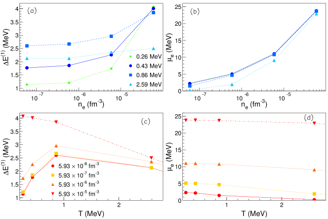
Figure 4: Evolution of $\Delta E^{(1)}$ as a function of $n_{e}$ (a) and $T$ (c) for constant values of $T$ and, respectively, $n_{e}$. Panels (b) and (d) illustrate the evolution of electron chemical potential $\mu_{e}$ under the same conditions as in panels (a) and (c).

In Fig. 4 (left panels) we show the evolution we obtain of $\Delta E^{(1)}$ with temperature and electron density, respectively. The fitted values lie between 1 and 4 MeV for all electron densities considered, indicating that the simple choice of a constant $\Delta E=2.5$ MeV in Ref. Langanke03 is a good first approximation.

Looking more in detail, the behavior of $\Delta E^{(1)}$ as a function of temperature (panel (c)) becomes more complex. This can be attributed to two competing effects. With increasing temperature, the contribution of excited states in the daughter nucleus increases, leading to a larger $\Delta E$. This effect is partly compensated by an electron chemical potential $\mu_{e}$ decreasing with temperature, see panel (d). Thus, depending on the value of $n_{e}$, $\Delta E^{(1)}$ can first increase and then decrease, or even show a monotonically decreasing behavior throughout the entire considered temperature range.

The increase of $\Delta E^{(1)}$ with $n_{e}$, see panel (a) of Fig. 4, can be attributed to the increase of $\mu_{e}$ with $n_{e}$, allowing for more excited states with higher energies to be populated. This effect is suppressed at the highest temperature by the decrease of $\mu_{e}$ with temperature, see above.

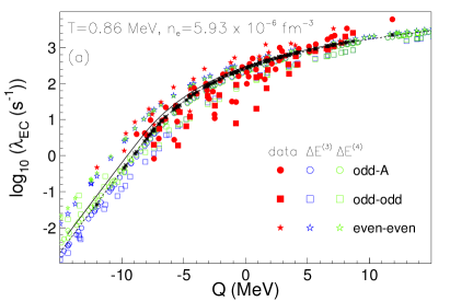
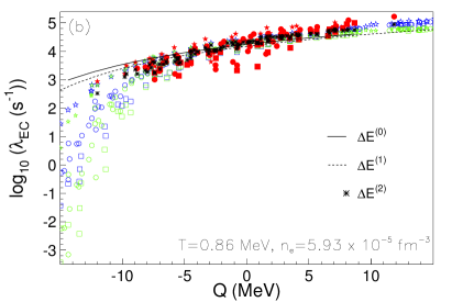
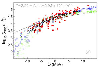
Figure 5: Electron capture rates: comparison between predictions of Eq. (1) with different prescriptions for the average transition energy $\Delta E$ (see text) and values of the tables from Ref. LMP . $\Delta E^{(0)}$ stands for the original parameterization of Ref. Langanke03 . The thermodynamic conditions, chosen from the grid points of weak interaction rates of Ref. LMP , are mentioned on each panel. The symbol and line legend is the same on the three panels.

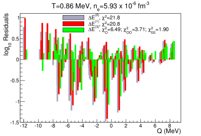
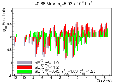
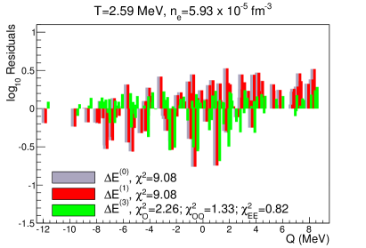
Figure 6: The residual differences between $\log_{10}$ of the shell model rates of Ref. LMP and the approximate rates for each nucleus in the weak interaction library calculated according to different recipes. The thermodynamical conditions, specified on each panel, are the same as in Fig. 5. To increase readability, for models (1) and (3) the $Q$-values have been shifted by 0.2 and, respectively, 0.4 MeV. In all cases, the $\chi^{2}$ values are mentioned in the key legend (see also Table I).

Altogether, allowing $\Delta E$ to depend on temperature and electron density only marginally improves the overall agreement of the parameterized rates with the microscopic ones, see Figs. 5 and 6. Fig. 5 displays a comparison of the EC rates from the calculations of Ref. LMP with the different parameterizations discussed here for several thermodynamic conditions. The plain lines corresponds to Eq. (1) and parameters from Ref. Langanke03 (model (0)) and the dashed line to model (1). In Fig. 6 the residual differences are shown. These simple parameterizations can clearly not reproduce the large scattering of the shell model rates due to the density of states of the daughter nucleus and the details of the GT strength distribution. Further refinements are thus necessary for a good description of EC rates.

In order to proceed, let us first note that the higher $\mu_{e}$, the less important become the details of nuclear structure. Therefore scattering of the rates is reduced with increasing $n_{e}$ and the parameterizations better reproduce the data (panels (a) and (b)). A similar effect occurs with increasing temperature, since nuclear structure effects are partially washed out by the increasing number of contributing excited states (panels (b) and (c)). It can be seen from Fig. 5, too, that the dependence of the EC rates on $Q$ considerably flattens with increasing temperature and electron density. As already observed in Langanke03 , this is due to the fact that the electron chemical potential increases with density much faster than the range of $Q$-values explored by the most abundant nuclei, again reducing the dependence on the detailed strength distribution. The capture process is thus dominated by the centroid of the GT-resonance.

Second, note that for high $T$ and $n_{e}$ values, a systematic deviation of the parameterizations with respect to the data of Ref. LMP can be observed (see Fig. 5, panels (b,c)): too high (low) EC rates for negative (positive) $Q$-values. A possible explanation for this deviation could be a residual isospin, $I=(N-Z)/A$, dependence of $\Delta E$ of the centroid of the GT resonance Juodagalvis05 ; Langanke00 ; Batist10 .

For this reason, in model (2) we further allow for a linear $I=(N-Z)/A$-dependence of $\Delta E$, see appendix A for details. The overall agreement of the parameterization with the data is considerably improved, see Fig. 5 and Table 1, even if at low temperatures noticeable deviations remain. This is due to the fact that the individual rates under these conditions depend on the details of the GT strength and it is thus not sufficient to reproduce global trends of the GT phenomenology.

A closer look at Fig.5 reveals that the dispersion of the individual rates is partially due to the existence of strong odd-even effects, see also the discussion in Ref. Langanke00 . We therefore introduce a separate parameterization of the average transition energy parameter $\Delta E$ for odd-odd (OO), even-even (EE) and odd-even (OE) nuclei, called model (3), see appendix A for details.

This extra refinement proves to be crucial for a good reproduction of shell-model calculations. As we can see from Table 1 (columns 11-13) and Figs. 5, 6, a sizeable reduction of the residuals is observed and data are well reproduced under all thermodynamic conditions considered here. Quite interesting, the relative ordering of the average transition energy parameter $\Delta E$ for OO,OE and EE nuclei is the same as the one of the GT₊ centroid energies of Ref. Langanke00 and does not seem to depend on the thermodynamic conditions.

In models (2) and (3) we assumed a linear isospin dependence of $\Delta E$, but this choice has to be considered as the leading term in an isospin dependence which is largely unknown. Indeed the limited $I$ range covered by present shell model calculations ($-0.07\leq I\leq 0.22$) makes it impossible to pin down the most appropriate functional trend. To demonstrate this statement, in model (4) we account for a quadratic dependence on isospin in addition to odd-even effects, see appendix A. The data are equally well reproduced by a model with a linear (model(3)) or a quadratic (model(4)) isospin dependence, see Figs. 5,6 and Table 1.

To conclude, we have discussed here several physically realistic effects Koonin94 susceptible to improve the description of microscopic EC rate calculations within a simple analytic parameterization. A possible dependence on temperature, electron density and isospin of the transition energy allow indeed for a better reproduction of data. Upon inclusion of odd-even effects, even the staggering of individual rates due to fluctuations in the GT strength distribution can be imitated.

Since microscopic data are better reproduced, we expect that the parameterizations discussed here provide, too, a better extrapolation to regions where no large scale shell model calculation exist for the moment. It was in particular demonstrated in Ref. Sullivan16 that in simulations the maximum sensitivity on individual rates concerns very neutron-rich nuclei around $N=50$. These nuclei lie in the lower right corner of Fig.3, with typical electron capture $Q$-values between -17 and -12 MeV. Those nuclei are abundantly produced in the later stage of the collapse, for densities $n_{e}\geq 1.4\cdot 10^{-4}$ fm^-3 and temperatures $T\geq 1.2$ MeV Sullivan16 ; Raduta16 .

We can see from Fig.5, that the more refined parameterizations, in particular models (2-4), predict an important reduction of the EC rate for these nuclei with respect to the reference parameterization from Ref. Langanke03 . To give a representative example, at $n_{e}=5.93\cdot 10^{-5}$ fm^-3 and $T=2.59$ MeV, model 3(4) predicts $\log_{10}(\lambda_{\mathrm{EC}})=1.69(0.32)$ for the even-even ⁷⁸Ni, $\log_{10}(\lambda_{\mathrm{EC}})=1.86(0.70)$ for the even-odd ⁷⁹Cu, and $\log_{10}(\lambda_{\mathrm{EC}})=2.49(1.72)$ for the odd-even ⁷⁹Zn, to be compared with $\log_{10}(\lambda_{\mathrm{EC}}({\rm{}^{78}Ni}))=3.11$, $\log_{10}(\lambda_{\mathrm{EC}}({\rm{}^{79}Cu}))=3.34$ and $\log_{10}(\lambda_{\mathrm{EC}}({\rm{}^{79}Zn}))=3.58$ obtained using a constant average value $\Delta E=2.5$ MeV from Ref.Langanke03 . We therefore expect a non-negligible influence on the global EC rate during core collapse, see the discussion in the following section.

IV NSE-averaged EC rates during core collapse

The effective reaction rate of a system composed of an ensemble of nuclei, as it is the case of finite-temperature dilute nuclear matter during core collapse, is the weighted sum of the contributions by individual nuclei:

$$\langle\lambda_{\mathrm{EC}}\rangle=\sum_{A,Z}n(A,Z)\lambda_{\mathrm{EC}}(A,Z)/\sum_{A,Z}n(A,Z)~{}.$$

Depending on the thermodynamic conditions, which affect both matter composition and individual reaction rates, a few tens of nuclei dominate the sum Sullivan16 .

As discussed in the previous section, the standard parameterization, Eq. (1), does not well describe EC on heavy neutron rich nuclei. In particular, allowing for an isospin and odd-even dependence may improve the reliability of the EC rates for those nuclei. To give an example of the impact this might have on the collapse, Fig. 7 shows the ratio of EC rates calculated according to models (0) and (3), across the nuclear chart for one representative thermodynamic condition ($T=1.4$ MeV, $n_{B}=3.52\cdot 10^{-4}$ fm^-3, $Y_{e}=0.32$). In the same figure, the contours give the isotopic abundances as predicted by NSE. For both $\left(\lambda_{\mathrm{EC}}^{(0)}(A,Z)/\lambda_{\mathrm{EC}}^{(3)}(A,Z)\right)$ and $n(A,Z)$ $\log_{10}$-scales are used. We can see that the improved parameterisation corresponds to both higher and lower rates with respect to the reference model, depending essentially on the isospin ratio. The most populated nuclear species show rates 1-3 orders of magnitude lower than model (0).

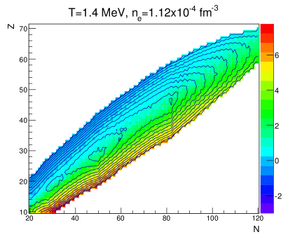
Figure 7: (Color online) $T=1.4$ MeV, $n_{B}=3.52\cdot 10^{-4}$ fm^-3, $Y_{e}=0.32$. Ratio between individual EC rates corresponding to models (0) and (3) (color levels) and isotopic multiplicities per unit volume (contours). For both $\left(\lambda_{EC}^{(0)}/\lambda_{EC}^{(3)}\right)$ and $n(N,Z)$ $\log_{10}$-scales are employed.

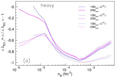
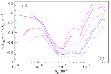
Figure 8: Ratio between NSE-averaged EC rates using models (2), (3) and (4) for the effective transition energy parameter $\Delta E$ (see Sec. III) and the fiducial parameterization of Ref. Langanke03 . The thermodynamic conditions correspond to the central element during core collapse of two progenitors with $15M_{\odot}$ and $25M_{\odot}$ Juodagalvis_2010 . The average rate is calculated only on heavy nuclei ($A\geq 20$) in panel (a) and on all nuclei in panel (b).

The actual modification of the rates along the trajectories is reported in Fig. 8. This figure shows the relative deviations in the NSE averaged EC rates of the improved parameterizations, models (2), (3) and (4), with respect to the fiducial model (0) from Ref. Langanke03 are depicted. Contributions of all (heavy) nuclei are considered separately.

The significant reduction of EC rates on heavy nuclei with large negative-$Q$ values, accounted for by the isospin dependent parameterizations, leads to a strong and almost systematic reduction of the associated average EC rate, see panel (a). In the first stage of the collapse this reduction is independent of the choice for the isospin dependence but depends strongly on whether odd-even effects are included or not. At this stage, nuclei with $Q\lesssim 0$ showing strong nuclear structure effects dominate EC explaining the sensitivity to odd-even effects. Isospin dependence is weak, since the range of populated $Q$-values is well constrained by microscopic data on $fp$-shell nuclei. In the late stages of the collapse electron capture reactions have processed the nuclear material into very neutron-rich matter and low $Y_{p}\lesssim 0.33$ values are reached. That stage corresponds to densities above $n_{B}\approx 2\cdot 10^{-4}$ fm^-3 (see fig. 3 of Ref. Raduta16 ). There, the isospin dependence dominates over structure details as can be seen from the similarity between the predictions of models (2) and (3). The stronger isospin dependence in model (4) leads to a considerably stronger reduction of the average EC rate on heavy nuclei with respect to model (3). As expected from Fig. 3, which shows that heavy nuclei produced in the central element of the two collapsing cores populate the same $Q$-value domain, the NSE average EC rates on heavy nuclei shows little sensitivity to the progenitor mass.

Panel (b) analyses EC rates NSE averaged over the whole nuclear distribution. It shows that, as long as, due to low temperatures, protons and light nuclei have low multiplicities, heavy nuclei clearly dominate EC. This corresponds to baryon number densities below roughly $4\cdot 10^{-5}$ fm^-3, where the mass fractions of protons and light nuclei do not exceed the percent level (see Ref. Raduta16 ). In the late stages of infall, when more protons and light nuclei are produced, a more moderate reduction of the overall rate is obtained. The progenitor dependence of $\langle\lambda_{\mathrm{EC}}^{all}\rangle$ is due to the progenitor dependence in the matter composition. According to Ref. Raduta16 the mass fraction bound in heavy nuclei is higher in the core of the progenitor with the smaller mass. Therefore higher deviations with respect to the fiducial model are obtained for the $15M_{\odot}$ progenitor than for the $25M_{\odot}$ one.

We recall that models (3) and (4) provide an equivalent fit to the available microscopic calculations and only differ in their extrapolation towards the extremely neutron-rich regime. This means that the difference between the dashed and the dotted curves in Fig.8 can be considered as an estimate of the present uncertainty due to unknown rates on extremely neutron rich nuclei. However a word of caution is in order. Other factors, such as temperature-dependent Pauli-blocking and structure effects that might occur far from stability, could strongly influence the strength distribution and depend on the region of nuclei investigated. As a consequence, the true uncertainty might even be larger. A correct extrapolation beyond the region covered by the shell-model EC tables available in the literature can only be done by confronting the predictions of our different phenomenological parameterizations to reliable microscopic EC calculations for extremely neutron rich nuclei, for instance with dedicated QRPA calculations QRPA ; inprep . If confirmed by microscopic calculations, this reduction of the EC rate on neutron rich nuclei in hot and dense environments would translate into higher electron fractions and entropies of the inner core together with increased masses at bounce and higher maxima of the neutrino luminosity peak Sullivan16 .

We note that the reduction of the averaged EC rates observed in this paper is opposite to the growth discussed in Ref. Raduta16 due to an expected magicity quenching towards the drip-line. Which is the dominant effect, which nuclei play the most important role and what exactly are the consequences on a core collapse trajectory are questions which can only be answered by core collapse simulations treating consistently nuclear abundances, individual EC rates, and neutrino dynamics. This task is beyond the present paper.

V Conclusions

In this paper we have investigated the role played by EC on neutron rich nuclei, abundantly produced in the late infall stages. To this aim, we have considered thermodynamic conditions corresponding to the trajectories of the central element, including a mass of 0.05$M_{\odot}$, of two progenitors with 15$M_{\odot}$ and 25$M_{\odot}$ masses during collapse Juodagalvis_2010 . Modifications of EC rates are considered perturbatively in this exploratory work, meaning that the time evolution of density, temperature and electron fraction is not modified while different prescriptions are considered for the EC rates.

EC rates have been calculated according to an analytic parameterization inspired by Ref. Langanke03 . Specifically, we seek for an optimal reproduction of large scale shell-model calculations considering a possible temperature, density, and isospin dependence of the effective average transition energy $\Delta E$. Odd-even effects are also included and shown to considerably improve the agreement with the microscopic data. Under the considered thermodynamic conditions, these new analytic parameterizations lead to an overall reduction of the NSE-averaged EC rate of up to one order of magnitude. This would imply, in an astrophysical simulation, larger electron fractions and entropies in the inner core and a larger mass at bounce. Though only an estimation due to the perturbative approximation of the present approach, the observed reduction of the EC rate is important enough to justify the effort for the calculation of accurate weak interaction rates on extremely neutron rich nuclei in hot and dense environments, constrained by new measurements of weak processes on exotic nuclei.

Appendix A Parameterizations of the electron capture rate

As mentioned in the text, we have employed four different parameterizations of the electron capture rate. Within this appendix we will detail the functional forms and the parameters employed.

We made a least-square fit of the EC tables of Ref. LMP at each grid point defined by a given value of temperature and electron density (see Fig.1). Since ${\mathcal{B}}$ gives only an overall normalization and does not change the functional dependence of the rate, we keep the fiducial value ${\mathcal{B}}=4.6$. Conversely, we allow $\Delta E$ to depend on $T$, $n_{e}$ and on the nuclear species, as it is physically reasonable to expect.

In model (1), the dependence on individual nuclei is neglected, but the average transition energy $\Delta E$ is assumed to depend on the temperature and electron density. Thus, instead of employing a global value of $\Delta E$, we determine for each couple $T(i),n_{e}(j)$ given in the tables of the microscopic calculations of Ref. LMP a different value,

$$\Delta E^{(1)}(n_{e}(i),T(j))=a_{i,j}~{}.$$ (2)

The parameter $a_{ij}$ is thereby fitted to the rates at temperature $T(i)$ and electron density $n_{e}(j)$.

The values of the fit parameters $a_{ij}$ are listed in Table 1 together with the corresponding $\chi^{2}$-values. The four considered temperatures and electron densities have been chosen since they are the most relevant for the CCSN trajectories we are interested in. They correspond to the highest values of the tables of Ref. LMP .

For thermodynamic conditions lying in between the grid points, $n_{e}(i)\leq n_{e}\leq n_{e}(i+1)$, $T(j)\leq T\leq T(j+1)$, a linear dependence is assumed,

$$\Delta E^{(1)}(n_{e},T) = Tn_{e}\frac{a_{i+1,j+1}-a_{i,j+1}-a_{i+1,j}+a_{i,j}}{\left[n_{e}(i+1)-n_{e}(i)\right]\left[T(j+1)-T(j)\right]}$$ (3)

$$+ n_{e}\frac{T(j+1)(a_{i,j+1}-a_{i,j})-T(j)(a_{i+1,j+1}-a_{i+1,j})}{\left[n_{e}(i+1)-n_{e}(i)\right]\left[T(j+1)-T(j)\right]}+T\frac{n_{e}(i+1)(a_{i+1,j}-a_{i,j})-n_{e}(i)(a_{i+1,j+1}-a_{i,j+1})}{\left[n_{e}(i+1)-n_{e}(i)\right]\left[T(j+1)-T(j)\right]}$$

$$+ \frac{n_{e}(i+1)T(j+1)a_{ij}-n_{e}(i+1)T(j)a_{i+1,j}-n_{e}(i)T(j+1)a_{i,j+1}+n_{e}(i)T(j)a_{i+1,j+1}}{\left[n_{e}(i+1)-n_{e}(i)\right]\left[T(j+1)-T(j)\right]}~{}.$$

In model (2) we allow for a possible $I=(N-Z)/A$-dependence of $\Delta E$ as:

$$\Delta E^{(2)}(n_{e}(i),T(j),I)=b_{i,j}I+c_{i,j}$$ (4)

Again as in model $(1)$, we assume a linear evolution of $\Delta E$ between different points $T(i),n_{e}(j)$ according to Eq. (3), upon replacing $a_{i,j}=b_{i,j}I+c_{i,j}$. Columns 8-10 in Table 1 provide, for the same temperature and electron density conditions as before, the $\chi^{2}$ values corresponding to this second scenario together with the values of $b_{i,j}$ and $c_{i,j}$. As expected, the extra degree of freedom leads to a better fit for all temperatures and/or densities expressed by lower $\chi^{2}$ values. The still relatively high values for $\chi^{2}$ obtained at the lowest considered temperatures arise due to fluctuations of individual rates, more than due to global trends in the Gamow-Teller phenomenology.

In model (3) we make a separate fit of the average transition energy parameter $\Delta E$ for odd-odd (OO), even-even (EE) and odd-even (OE) nuclei:

$$\Delta E^{(3)}_{OO}(n_{e}(i),T(j),I) = b_{i,j}^{OO}I+c_{i,j}^{OO},$$ (5)

$$\Delta E^{(3)}_{OE}(n_{e}(i),T(j),I) = b_{i,j}^{OE}I+c_{i,j}^{OE},$$ (6)

$$\Delta E^{(3)}_{EE}(n_{e}(i),T(j),I) = b_{i,j}^{EE}I+c_{i,j}^{EE}~{}.$$ (7)

As we can see from Table 1 (columns 11-13), the fit is considerably improved and very reasonable $\chi^{2}$ are obtained for all thermodynamic conditions considered here.

The isospin dependence of $\Delta E(I)$ is largely unknown, and the linear choice of model (2) and model (3), see Eqs.(4-7), has to be considered as the leading term. In model (4) we introduce a quadratic isospin dependence,

$$\Delta E^{(4)}_{OO}(n_{e}(i),T(j),I) = b_{i,j}^{OO}I^{2}+c_{i,j}^{OO},$$ (8)

$$\Delta E^{(4)}_{OE}(n_{e}(i),T(j),I) = b_{i,j}^{OE}I^{2}+c_{i,j}^{OE},$$ (9)

$$\Delta E^{(4)}_{EE}(n_{e}(i),T(j),I) = b_{i,j}^{EE}I^{2}+c_{i,j}^{EE}$$ (10)

We can see from Table  1 (columns 14-16) that linear and quadratic $I$-dependence of $\Delta E$ lead to similar $\chi^{2}$ values.

$T$	$n_{e}$	$\mu_{e}$	$\Delta E^{(0)}$		$\Delta E^{(1)}$		$\Delta E^{(2)}$			$\Delta E^{(3)}$			$\Delta E^{(4)}$
(MeV)	(fm-3)	(MeV)	$\Delta E$	$\chi^{2}$	$\Delta E$	$\chi^{2}$	$b$	$c$	$\chi^{2}$	$b$	$c$	$\chi^{2}$	$b$	$c$	$\chi^{2}$
0.43	$5.93\times 10^{-8}$	2.18	2.5	$1.22\times 10^{2}$	1.77	$9.68\times 10^{1}$	$-1.42\times 10^{1}$	3.31	$7.74\times 10^{1}$	$-2.01\times 10^{1}$	4.11	$1.06\times 10^{1}$	$-9.63\times 10^{1}$	3.23	$1.32\times 10^{1}$
										$-2.97\times 10^{1}$	6.69	5.83	$-1.38\times 10^{2}$	5.35	6.42
										$-1.67\times 10^{1}$	2.25	1.89	$-8.24\times 10^{1}$	1.58	2.94
0.43	$5.93\times 10^{-7}$	5.03	2.5	$1.05\times 10^{2}$	1.86	$9.01\times 10^{1}$	$-1.37\times 10^{1}$	3.50	$7.95\times 10^{1}$	$-2.26\times 10^{1}$	4.85	$1.64\times 10^{1}$	$-1.04\times 10^{2}$	3.77	$1.74\times 10^{1}$
										$-3.46\times 10^{1}$	7.83	$1.00\times 10^{1}$	$-1.62\times 10^{2}$	6.30	9.14
										$-1.78\times 10^{1}$	2.66	3.38	$-8.28\times 10^{1}$	1.83	3.88
0.43	$5.93\times 10^{-6}$	$1.10\times 10^{1}$	2.5	$4.00\times 10^{1}$	2.26	$3.93\times 10^{1}$	$-8.26$	3.37	$3.85\times 10^{1}$	$-1.07\times 10^{1}$	4.34	$1.22\times 10^{1}$	$-6.00\times 10^{1}$	4.05	$1.20\times 10^{1}$
										$-2.26\times 10^{1}$	7.54	6.18	$-1.16\times 10^{2}$	6.92	5.35
										$-9.58$	2.40	3.38	$-5.01\times 10^{1}$	2.09	3.22
0.43	$5.93\times 10^{-5}$	$2.38\times 10^{1}$	2.5	$1.25\times 10^{1}$	4.01	$1.15\times 10^{1}$	5.28 $\times 10^{1}$	$-1.87$	7.64	$5.40\times 10^{1}$	$-1.70$	3.68	$2.46\times 10^{2}$	$6.62\times 10^{-1}$	4.12
										$4.53\times 10^{1}$	$7.90\times 10^{-1}$	1.70	$1.77\times 10^{2}$	3.24	1.95
										$5.21\times 10^{1}$	$-3.16$	1.42	$2.29\times 10^{2}$	$-8.12\times 10^{-1}$	1.65
0.86	$5.93\times 10^{-8}$	1.48	2.5	$3.54\times 10^{1}$	2.6	$3.53\times 10^{1}$	$-1.04\times 10^{1}$	3.62	$3.19\times 10^{1}$	$-1.50\times 10^{1}$	4.22	3.51	$-8.61\times 10^{1}$	3.77	3.44
										$-1.86\times 10^{1}$	6.52	2.75	$-1.05\times 10^{2}$	5.97	2.18
										$-1.37\times 10^{1}$	2.06	$8.01\times 10^{-1}$	$-7.55\times 10^{1}$	1.61	$8.83\times 10^{-1}$
0.86	$5.93\times 10^{-7}$	4.68	2.5	$3.28\times 10^{1}$	2.67	$3.25\times 10^{1}$	$-8.19$	3.56	3.10 $\times 10^{1}$	$-1.46\times 10^{1}$	4.47	5.05	$-8.29\times 10^{1}$	4.01	4.69
										$-2.00\times 10^{1}$	6.99	3.85	$-1.12\times 10^{2}$	6.41	3.16
										$-1.28\times 10^{1}$	2.24	1.16	$-7.01\times 10^{1}$	1.79	1.11
0.86	$5.93\times 10^{-6}$	$1.08\times 10^{1}$	2.5	$2.18\times 10^{1}$	2.96	$2.08\times 10^{1}$	1.94	2.72	2.08 $\times 10^{1}$	$-1.52$	3.56	6.49	$-2.07\times 10^{1}$	3.72	6.43
										$-1.06\times 10^{1}$	6.39	3.71	$-7.00\times 10^{1}$	6.37	3.43
										$-1.76$	1.60	1.90	$-2.07\times 10^{1}$	1.73	1.87
0.86	$5.93\times 10^{-5}$	$2.37\times 10^{1}$	2.5	$1.19\times 10^{1}$	3.85	$1.12\times 10^{1}$	$5.57\times 10^{1}$	$-2.25$	7.20	$5.64\times 10^{1}$	$-2.03$	3.45	$2.59\times 10^{2}$	$3.95\times 10^{-1}$	3.89
										$4.85\times 10^{1}$	$4.52\times 10^{-1}$	1.63	$1.93\times 10^{2}$	3.00	1.89
										$5.37\times 10^{1}$	$-3.54$	1.25	$2.39\times 10^{2}$	$-1.16$	1.47
2.59	$5.93\times 10^{-8}$	$2.05\times 10^{-1}$	2.5	7.25	2.13	7.11	$1.16\times 10^{1}$	1.10	6.67	8.09	1.46	1.52	$3.02\times 10^{1}$	1.85	1.59
										$1.34\times 10^{1}$	3.42	1.48	$4.83\times 10^{1}$	4.14	1.56
										4.62	$-6.65\times 10^{-1}$	$5.33\times 10^{-1}$	$1.71\times 10^{1}$	$-4.44\times 10^{-1}$	$5.43\times 10^{-1}$
2.59	$5.93\times 10^{-7}$	1.94	2.5	7.36	2.13	7.22	$1.35\times 10^{1}$	$8.94\times 10^{-1}$	6.69	9.61	1.31	1.61	$3.34\times 10^{1}$	1.82	1.70
										$1.39\times 10^{1}$	3.37	1.50	$4.85\times 10^{1}$	4.16	1.59
										5.83	$-7.65\times 10^{-1}$	$5.58\times 10^{-1}$	$2.07\times 10^{1}$	$-4.67\times 10^{-1}$	$5.72\times 10^{-1}$
2.59	$5.93\times 10^{-6}$	9.09	2.5	7.70	2.36	7.69	$2.63\times 10^{1}$	$-2.90\times 10^{-1}$	6.27	$2.24\times 10^{1}$	$2.09\times 10^{-1}$	1.94	$9.49\times 10^{1}$	1.27	2.16
										$2.34\times 10^{1}$	2.45	1.54	$8.92\times 10^{1}$	3.72	1.68
										$1.91\times 10^{1}$	$-1.74$	$6.75\times 10^{-1}$	$8.35\times 10^{1}$	$-8.86\times 10^{-1}$	$7.44\times 10^{-1}$
2.59	$5.93\times 10^{-5}$	$2.29\times 10^{1}$	2.5	9.08	2.50	9.08	$7.24\times 10^{1}$	-4.75	5.07	$6.92\times 10^{1}$	$-4.34$	2.26	$3.34\times 10^{2}$	-1.65	2.66
										$6.82\times 10^{1}$	$-2.10$	1.33	$2.95\times 10^{2}$	1.02	1.58
										$6.71\times 10^{1}$	$-5.99$	$8.23\times 10^{-1}$	$3.23\times 10^{2}$	$-3.41$	$9.93\times 10^{-1}$
8.62	$5.93\times 10^{-8}$	$1.84\times 10^{-2}$	2.5	8.17	-1.87	6.85	$1.01\times 10^{2}$	$-9.99$	4.51	$9.17\times 10^{1}$	$-9.16$	2.17	$5.05\times 10^{2}$	$-6.72$	2.43
										$1.23\times 10^{2}$	$-9.03$	1.12	$6.16\times 10^{2}$	$-5.00$	1.30
										$7.26\times 10^{1}$	$-1.06\times 10^{1}$	$7.64\times 10^{-1}$	$3.72\times 10^{2}$	$-8.44$	$8.60\times 10^{-1}$
8.62	$5.93\times 10^{-7}$	$1.84\times 10^{-1}$	2.5	8.17	$-1.86$	6.85	$1.01\times 10^{2}$	$-1.00\times 10^{1}$	4.50	$9.19\times 10^{1}$	$-9.18$	2.17	$5.05\times 10^{2}$	$-6.72$	2.43
										$1.23\times 10^{2}$	$-9.05$	1.12	$6.16\times 10^{2}$	$-5.00$	1.30
										$7.27\times 10^{1}$	$-1.06\times 10^{1}$	$7.62\times 10^{-1}$	$3.72\times 10^{2}$	$-8.44$	$8.58\times 10^{-1}$
8.62	$5.93\times 10^{-6}$	1.83	2.5	8.16	$-1.83$	6.87	$1.03\times 10^{2}$	$-1.02\times 10^{1}$	4.52	$9.35\times 10^{1}$	$-9.35$	2.17	$5.08\times 10^{2}$	$-6.75$	2.45
										$1.24\times 10^{2}$	$-9.20$	1.12	$6.17\times 10^{2}$	$-5.02$	1.31
										$7.39\times 10^{1}$	$-1.07\times 10^{1}$	$7.67\times 10^{-1}$	$3.75\times 10^{2}$	$-8.46$	$8.65\times 10^{-1}$
8.62	$5.93\times 10^{-5}$	$1.44\times 10^{1}$	2.5	8.43	$-2.17$	7.21	$1.23\times 10^{2}$	$-1.25\times 10^{1}$	4.55	$1.14\times 10^{2}$	$-1.16\times 10^{1}$	2.22	$5.93\times 10^{2}$	$-8.04$	2.53
										$1.43\times 10^{2}$	$-1.14\times 10^{1}$	1.13	$6.86\times 10^{2}$	$-6.19$	1.34
										$9.13\times 10^{1}$	$-1.26\times 10^{1}$	$7.87\times 10^{-1}$	$4.50\times 10^{2}$	$-9.61$	$9.02\times 10^{-1}$

Table 1: Values of $\Delta E$-parameter (MeV) of Eq. (1) extracted by fitting shell model EC rates of Ref. LMP under different hypothesis (see text) and for various thermodynamic conditions mentioned in columns 1 and 2. In case of models $(3)$ and $(4)$, values of odd-even, odd-odd and even-even parameters are given respectively in rows 1, 2, 3. $\mu_{e}$ represents the electron chemical potential and includes the rest mass.

References

- (1) S. Goriely, A. Bauswein, O. Just, E. Pllumbi and H. T. Janka, Mon. Not. Roy. Astron. Soc. 452, 3894 (2015).
- (2) S. Gupta, E. F. Brown, H. Schatz, P. Moeller and K. L. Kratz, Astrophys. J. 662, 1188 (2007).
- (3) H. Schatz et al., Nature 505, 7481, 62 (2014).
- (4) K. Iwamoto, F. Brachwitz, K. Nomoto, et al. , ApJS 125, 439 (1999).
- (5) F. Brachwitz et al., Astrophys. J. 536, 934 (2000).
- (6) M. B. Aufderheide, I. Fushiki, S. E. Woosley, D. A. Hartmann, Astrophys. Journ. Suppl. 91, 389 (1994).
- (7) A. Heger, K. Langanke, G. Martinez-Pinedo, S.E. Woosley, Phys. Rev. Lett. 86, 1678 (2001); A. Heger, S. E. Woosley, G. Martinez-Pinedo, K. Langanke, Astrophys. J. 560, 307 (2001).
- (8) W. R. Hix, O. E. B. Messer, A. Mezzacappa, M. Liebendörfer, J. Sampaio, K. Langanke, D. J. Dean, and G. Martinez-Pinedo, Phys. Rev. Lett. 91, 201102 (2003).
- (9) H. T. Janka, K. Langanke, A. Marek, G. Martinez-Pinedo and B. Mueller, Phys. Rept. 442, 38 (2007).
- (10) K. Langanke et al., Phys. Rev. Lett. 90, 241102 (2003).
- (11) A. R. Raduta, F. Gulminelli and M. Oertel, Phys. Rev. C 93, 025803 (2016).
- (12) C. Sullivan, E. O’Connor, R. G. T. Zegers, T. Grubb, and S. A. Austin, ApJ 816, 44 (2016).
- (13) K. Langanke and G. Martinez-Pinedo, Atomic Data and Nuclear Data Tables 79, 1 (2001).
- (14) T. Oda, M. Hino, K. Muto, M. Takahara, and K. Sato, At. Data Nucl. Data Tables 56, 231 (1994).
- (15) A. Juodagalvis, K. Langanke, W.R. Hix, G. Martinez-Pinedo, J.M. Sampaio, Nucl. Phys. A848, 454 (2010).
- (16) F. Gulminelli and A. R. Raduta, Phys. Rev. C 92, 055803 (2015).
- (17) G. Audi, M. Wang, A. H. Wapstra, F. G. Kondev, M. MacCormick, X. Xu, and B. Pfeiffer, Chinese Physics C36, 1287 (2012); M. Wang, G. Audi, A. H. Wapstra, F. G. Kondev, M. MacCormick, X. Xu, and B. Pfeiffer, Chinese Physics C36, 1603 (2012); http://amdc.impcas.ac.cn/evaluation/data2012/data/nubase.mas12.
- (18) J. Duflo and A. P. Zuker, Phys. Rev. C 52, R23 (1995); http://amdc.in2p3.fr/web/dz.html.
- (19) K. Langanke and G. Martinez-Pinedo, Nucl. Phys. A673, 481 (2000).
- (20) A. Juodagalvis and D. J. Dean, Phys. Rev. C 72, 024306 (2005).
- (21) L. Batist, M. Gorska, H. Grawe, Z. Janas, M. Kavatsyuk, M. Karny, R. Kirchner, M. La Commara, I. Mukha, A. Plochocki, and E. Roeckl, Eur. Phys. J. A 46, 45 (2010).
- (22) P. Goldreich and S.V. Weber, Astrophys. J. 238, 991 (1980).
- (23) A. Yahil, Ap. J. 265, 1047 (1983).
- (24) S. W. Bruenn, ApJS 58, 771 (1985).
- (25) G. M. Fuller, W. A. Fowler, M. J. Newman, ApJS 42, 447 (1980); G. M. Fuller, W. A. Fowler, M. J. Newman, ApJS 48, 279 (1982).
- (26) G. M. Fuller, W. A. Fowler and M. J. Newman, ApJ 252, 715 (1982).
- (27) G. M. Fowler, W. A. Fuller, M. J. Newman, Astrophys. J. 293, 1 (1985).
- (28) G. M. Fuller and C. J. Smith, Phys. Rev. D 82, 125017 (2010).
- (29) G. Martinez-Pinedo, Y. H. Lam, K. Langanke, R. G. T. Zegers and C. Sullivan, Phys. Rev. C 89, 045806 (2014).
- (30) J. Nabi and H. V. Klapdor-Kleingrothaus, Atomic Data and Nuclear Data Tables 71, 149 –345 (1999); ibid., Atomic Data and Nuclear Data Tables 88, 237–476 (2004).
- (31) A. F. Fantina, E. Khan, G. Colo, N. Paar and D. Vretenar, Phys. Rev. C 86, 035805 (2012).
- (32) N. Paar, G. Colo, E. Khan and D. Vretenar, Phys. Rev. C 80, 055801 (2009); Y. F. Niu, N. Paar, D. Vretenar and J. Meng, Phys. Rev. C 83, 045807 (2011).
- (33) L. Cole, T. S. Anderson, R. G. T. Zegers et al., Phys. Rev. C 86, 015809 (2012).
- (34) J. Pruet and G. M. Fuller, Astrophys. J. Suppl. Ser. 149, 189 (2003).
- (35) J. C. Hardy and I. S. Towner, Phys. Rev. C 79, 055502 (2009).
- (36) S.E. Koonin and K. Langanke, Phys. Lett. B 326, 5 (1994).
- (37) A. Fantina et al., in preparation.