Dual polynomial spline bases

Abstract

In the paper, we give methods of construction of dual bases for the B-spline basis and truncated power basis. Explicit formulas for the dual B-spline basis are obtained using the Legendre-like orthogonal basis of the polynomial spline space presented in (Wei et al., Comput.-Aided Des. 45 (2013), 85–92) and a connection between orthogonal and dual bases of any space given in (Lewanowicz and Woźny, J. Approx. Theory 138 (2006), 129–150). Construction of the dual truncated power basis is performed in two phases. We start with explicit formulas for the dual power basis of the space of polynomials. Then, we expand this basis using an iterative algorithm proposed in (Woźny, J. Comput. Appl. Math. 260 (2014), 301–311). As a result, we obtain the dual truncated power basis. We also present some applications of the proposed dual polynomial spline bases and illustrative examples.

1 Introduction

Recently, dual bases with their applications in numerical analysis and computer graphics have been extensively studied. For example, there are many articles concerning the dual Bernstein polynomials (see, e.g., Cie87 ; Jue98 ) and their applications in several important algorithms associated with Bézier curves (see, e.g., BJ07 ; GLW15 ; GLW17 ; LWK12 ; Liu09 ; WGL15 ; WL09 ). Moreover, one can find some general results on dual bases (see GW15 ; Ker13 ; Woz13 ; Woz14 ). Nevertheless, the number of articles concerning dual polynomial spline bases is still very limited. In Woz14 , an iterative method of construction of the dual B-spline basis was presented.

There are several important approximation problems concerning polynomial spline curves, e.g., degree reduction (see, e.g., Hos87 ; LP01 ; PW09 ; PT95 ; WWF98 ; Woz14 ; Yong01 ), merging (see, e.g., CW10 ; THH03 ) and knots removal (see, e.g., Eck95 ; LM87 ; Woz14 ). In order to solve these problems using least squares approximation, it is helpful to know the dual basis for the selected polynomial spline basis (see (Woz14, , §4)).

The first goal of the paper is to give a new method of construction of the dual B-spline basis. In contrast to the iterative method presented in Woz14 , our aim is to provide explicit formulas for the dual B-spline functions. Another difference is that the previous approach is based on a more general algorithm of construction of dual basis with respect to an arbitrary inner product, whereas the new method is fully adjusted to the B-spline basis, and the $L_{2}$ inner product on the interval $[0,\,1]$ is selected. The idea is to use a certain connection between orthogonal and dual bases of any space. As we shall see in §2.1, a well-expressed orthogonal basis of a polynomial spline space is needed. There are several papers dealing with the construction of orthogonal bases of various polynomial spline spaces (see, e.g., FHRS96 ; KTM88 ; MRS93 ; Red12 ; Sab88 ; Sch75 ; WGY13 ). In contrast to the other methods, the one given in WGY13 provides a well-expressed orthogonal basis of the polynomial spline space defined over an arbitrary knot vector (see §2.2). Consequently, it is used in our method of construction of the dual B-spline basis. Moreover, we have noted that in WGY13 , there are no formulas connecting the B-spline basis and the presented orthogonal basis. As it turns out, such formulas lead to the dual B-spline basis, and they are useful in solving least squares approximation problems concerning B-spline curves. For details, see §3.

The second goal of the paper is to construct the dual basis for the truncated power basis of the polynomial spline space. The idea is to start with the construction of the dual basis for the power basis of the space of polynomials. We give explicit formulas for those dual power functions. Then, in order to obtain the dual truncated power basis, we can expand the dual power basis using the iterative algorithm from Woz14 . For details, see §4. According to the authors‘ knowledge, methods of construction of the dual power basis and dual truncated power basis have never been published before.

In §5, we explain the applications of the proposed dual polynomial spline bases in degree reduction and knots removal for spline curves. We also give some illustrative examples.

2 Preliminaries

2.1 Dual and orthogonal bases

Let $B_{n}:=\left\{b_{0},b_{1},\ldots,b_{n}\right\}$ be a basis of the linear space $\mathcal{B}_{n}:=\mbox{span}\,B_{n}$. The dual basis $D_{n}:=\left\{d_{0}^{(n)},d_{1}^{(n)},\ldots,d_{n}^{(n)}\right\}$ for the basis $B_{n}$ of the space $\mathcal{B}_{n}$ satisfies the following duality conditions:

$$\mbox{span}\,D_{n}=\mathcal{B}_{n},$$

$$\left<b_{i},d_{j}^{(n)}\right>=\delta_{i,j}\qquad(i,j=0,1,\ldots,n),$$

where $\left<\cdot,\cdot\right>\,:\,\mathcal{B}_{n}\times\mathcal{B}_{n}\rightarrow\mathbb{R}$ is an inner product, and $d_{j}^{(n)}$ $(j=0,1,\ldots,n)$ are called dual functions. Here $\delta_{i,j}$, known as Kronecker delta, equals $1$ if $i=j$, and $0$ otherwise.

Let $q_{0},q_{1},\ldots,q_{n}$ be an orthogonal basis of the space $\mathcal{B}_{n}$ with respect to the inner product $\left<\cdot,\cdot\right>$, i.e., the following conditions are satisfied:

$$\mbox{span}\,\{q_{0},q_{1},\ldots,q_{n}\}=\mathcal{B}_{n},$$

$$\left<q_{i},q_{j}\right>=h_{i}\delta_{i,j}\qquad(h_{i}>0;\,i,j=0,1,\ldots,n).$$

Recall that orthogonal and dual bases of any space are related.

Lemma 2.1 (LW06 ).

Suppose that we know the representation of each $q_{0},q_{1},\ldots,q_{n}$ in the basis $b_{0},b_{1},\ldots,b_{n}$,

$$q_{i}=\sum_{j=0}^{n}a_{i,j}b_{j}\qquad(i=0,1,\ldots,n).$$

Then, the dual functions $d_{0}^{(n)},d_{1}^{(n)},\ldots,d_{n}^{(n)}$ can be written in the following way:

$$d_{j}^{(n)}=\sum_{i=0}^{n}h_{i}^{-1}a_{i,j}q_{i}\qquad(j=0,1,\ldots,n).$$

Now, we recall the well-known fact about the use of dual and orthogonal bases in least squares approximation.

Fact 2.2 (e.g., Woz13 and (DB08, , Theorem 4.5.13)).

The element

$$p_{n}^{\ast}:=\sum_{i=0}^{n}\left<f,d_{i}^{(n)}\right>b_{i}=\sum_{i=0}^{n}\frac{\left<f,q_{i}\right>}{\left<q_{i},q_{i}\right>}q_{i}$$

is the best least squares approximation of a function $f$ in the space $\mathcal{B}_{n}$, i.e.,

$$\|f-p_{n}^{\ast}\|=\min_{p_{n}\in\mathcal{B}_{n}}\|f-p_{n}\|,$$

where $\|\cdot\|:=\sqrt{\left<\cdot,\cdot\right>}$ is the least squares norm.

According to Fact 2.2, the use of an orthogonal basis in the least squares approximation implies that the resulting $p_{n}^{\ast}$ will be written in this orthogonal basis. If a different representation for $p_{n}^{\ast}$ is required, then additional conversion is necessary. Observe that an appropriate dual basis is more convenient in this regard because we get the resulting $p_{n}^{\ast}$ in the chosen basis, and the additional conversion is not required. Moreover, the dual basis approach may lead to some algorithms having lower computational complexity (see, e.g., GLW15 ; GLW17 ; WGL15 ; WL09 ).

2.2 Polynomial spline bases

Let $\Omega_{n}[T_{m}]$ be the space of polynomial spline curves of degree at most $n$ defined over the knot vector

$$T_{m} :=\big{(}\underbrace{0,0,\ldots,0}_{n+1}<t_{1}\leq t_{2}\leq\cdots\leq t_{m}<\underbrace{1,1,\ldots,1}_{n+1}\big{)}$$ (2.1)

$$\equiv\left(t_{-n}^{(m)},t_{-n+1}^{(m)},\ldots,t_{n+m+1}^{(m)}\right),$$

where $t_{1},t_{2},\ldots,t_{m}$ are called interior knots. We assume that the multiplicity of an interior knot does not exceed $n$. The (normalized) B-spline basis of the space $\Omega_{n}[T_{m}]$,

$$N_{-n,n}^{m},N_{-n+1,n}^{m},\ldots,N_{m,n}^{m},$$ (2.2)

can be defined recursively,

$$N_{i,0}^{m}(t):=\left\{\begin{array}[]{ll}1&\left(t_{i}^{(m)}\leq t<t_{i+1}^{(m)}\right),\\[4.30554pt] 0&\text{otherwise},\end{array}\right.$$

$$N_{i,n}^{m}(t):=\frac{t-t_{i}^{(m)}}{t_{i+n}^{(m)}-t_{i}^{(m)}}N_{i,n-1}^{m}(t)+\frac{t_{i+n+1}^{(m)}-t}{t_{i+n+1}^{(m)}-t_{i+1}^{(m)}}N_{i+1,n-1}^{m}(t);$$

and explicitly,

$$N_{i,n}^{m}(t):=\left(t_{i+n+1}^{(m)}-t_{i}^{(m)}\right)\left[t_{i}^{(m)},t_{i+1}^{(m)},\ldots,t_{i+n+1}^{(m)}\right](\cdot-t)^{n}_{+},$$

where

$$(x-t)^{n}_{+}:=\left\{\begin{array}[]{ll}\displaystyle(x-t)^{n}&(x>t),\\[4.30554pt] \displaystyle 0&(x\leq t).\end{array}\right.$$

Here $\left[x_{1},x_{2},\ldots,x_{k}\right]f$ is a divided difference (see, e.g., (DB08, , §4.2.1)). At an interior knot $N_{i,n}^{m}(t)$ is $n-k$ times continuously differentiable, where $k$ is the multiplicity of the interior knot. For some other useful properties of the B-spline basis, we recommend (PT97, , §2).

In the paper, $\Pi_{n}$ denotes the space of all polynomials of degree at most $n$. Observe that $\Pi_{n}\equiv\Omega_{n}[T_{0}]$ on $[0,1]$, where

$$T_{0}:=\big{(}\underbrace{0,0,\ldots,0}_{n+1},\underbrace{1,1,\ldots,1}_{n+1}\big{)}.$$

The well-known power basis

$$1,t,\ldots,t^{n}$$ (2.3)

of the space $\Pi_{n}$, and the functions

$$(t-t_{q})^{n-h}_{+}\qquad(h=0,1,\ldots,l_{q}-1)$$

for each interior knot $t_{q}$ of multiplicity $l_{q}$ $(1\leq l_{q}\leq n)$ in $T_{m}$ form the truncated power basis of the space $\Omega_{n}[T_{m}]$. For example, let us assume that there is only one multiple interior knot $t_{r}$, i.e., we consider

$$T^{\prime}_{m}:=\big{(}\underbrace{0,0,\ldots,0}_{n+1}<t_{1}<t_{2}<\cdots<t_{r}=t_{r+1}=\cdots=t_{r+l_{r}-1}<t_{r+l_{r}}<\cdots<t_{m}<\underbrace{1,1,\ldots,1}_{n+1}\big{)}.$$

Then, the functions (2.3),

$$(t-t_{j})^{n}_{+}\qquad(j=1,2,\ldots,r-1,r+l_{r},\ldots,m),$$

$$(t-t_{r})^{n-h}_{+}\qquad(h=0,1,\ldots,l_{r}-1)$$

form the truncated power basis of the space $\Omega_{n}[T^{\prime}_{m}]$.

Further on in the paper, the inner product $\left<\cdot,\cdot\right>_{L}\,:\,\Omega_{n}[T_{m}]\times\Omega_{n}[T_{m}]\rightarrow\mathbb{R}$ is defined as follows:

$$\langle f,g\rangle_{L}:=\int_{0}^{1}f(t)g(t)\mbox{${\rm\,d}t$}.$$ (2.4)

In §3, we will need a well-expressed orthogonal basis of the space $\Omega_{n}[T_{m}]$ with respect to the inner product (2.4) (cf. Lemma 2.1). Therefore, we recall the formulas given in WGY13 .

Lemma 2.3 (WGY13 ).

Legendre-like orthogonal basis of the space $\Omega_{n}[T_{m}]$ with respect to the inner product (2.4) is given by

$$L_{i,n}(t):=\frac{1}{i!}\frac{\mbox{${\rm\,d}$}^{i}(1-t)^{i}t^{i}}{\mbox{${\rm\,d}t$}^{i}}\qquad(i=0,1,\ldots,n),$$ (2.5)

$$L_{n+k,n}(t):=\frac{\mbox{${\rm\,d}$}^{n+1}}{\mbox{${\rm\,d}t$}^{n+1}}f_{k}(t)\qquad(k=1,2,\ldots,m),$$ (2.6)

where

$$f_{k}(t):=\sum_{j=0}^{k-1}\alpha_{-n+j,k}N_{-n+j,2n+1}^{k}(t)$$

with $\alpha_{-n+j,k}$ as defined in (WGY13, , (2) and (3)).

Legendre polynomials $P_{i}$ $(i=0,1,\ldots)$, which are a special case of Jacobi polynomials, can be represented using the hypergeometric function (see, e.g., (AAR99, , p. 117)),

$$P_{i}(x)=(-1)^{i}{}_{2}F_{1}\left({\textstyle-i,\,i+1\atop\textstyle 1}\,\middle|\,\frac{1+x}{2}\right),$$ (2.7)

where

$${}_{2}F_{1}\left({\textstyle-s,\,a\atop\textstyle b}\,\middle|\,t\right):=\sum_{k=0}^{s}\frac{(-s)_{k}(a)_{k}}{(b)_{k}k!}t^{k}\qquad(s\in\mathbb{N})$$ (2.8)

with

$$(h)_{0}:=1,\qquad(h)_{k}:=h(h+1)\cdots(h+k-1).$$

The functions

$$L_{i,n}(t)\equiv(-1)^{i}P_{i}(2t-1)\qquad(i=0,1,\ldots,n)$$ (2.9)

are called shifted Legendre polynomials (cf. (2.5)).

3 Dual B-spline basis

3.1 Explicit formulas for the dual B-spline basis

In this section, our goal is to construct the dual basis for the B-spline basis (2.2) of the space $\Omega_{n}[T_{m}]$ with respect to the inner product (2.4). The idea is to use Lemmas 2.1 and 2.3. To do so, we will represent each $L_{j,n}$ $(j=0,1,\ldots,n+m)$ (see (2.5) and (2.6)) in the B-spline basis (2.2) of the space $\Omega_{n}[T_{m}]$. Note that the given formulas are explicit.

Lemma 3.1.

The shifted Legendre polynomials $L_{i,n}$ $(i=0,1,\ldots,n)$ (see (2.5)) can be written in terms of the B-spline functions of degree $n$ over the knot vector $T_{m}$ (see (2.2)),

$$L_{0,n}(t)=\sum_{j=0}^{n+m}N_{-n+j,n}^{m}(t),$$ (3.1)

$$L_{i,n}(t)=\sum_{j=0}^{n+m}\phi_{j,i}N_{-n+j,n}^{m}(t)\qquad(i=1,2,\ldots,n),$$ (3.2)

where

$$\phi_{j,i}:=\sum_{h=0}^{i}\frac{(-i)_{h}(i+1)_{h}}{\binom{n}{h}(h!)^{2}}\sum_{\begin{subarray}{c}S\subset A_{j}\\ |S|=h\end{subarray}}\;\prod_{s\in S}t_{s}^{(m)}$$ (3.3)

with $A_{j}:=\left\{-n+j+1,-n+j+2,\ldots,j\right\}$.

Proof.

First, it is well known that the B-spline functions form a partition of unity, the formula (3.1) is thus proven. Next, we obtain

$$L_{i,n}(t)=\sum_{h=0}^{i}(-i)_{h}(i+1)_{h}(h!)^{-2}t^{h}\qquad(i=1,2,\ldots,n)$$ (3.4)

using (2.9), (2.7) and (2.8). The polynomials $L_{i,n}$ $(i=1,2,\ldots,n)$ are now written in the monomial form, but we need to represent them in the basis (2.2) of the space $\Omega_{n}[T_{m}]$. Such a conversion can be performed using the polar forms of $\binom{n}{h}t^{h}$ $(h=0,1,\ldots,n)$. This approach generalizes the Marsden‘s identity (see, e.g., (PBP02, , §5.8)). As a result, we obtain (3.2). ∎

Lemma 3.2.

The functions $L_{n+k,n}$ $(k=1,2,\ldots,m)$ (see (2.6)) can be written in terms of the B-spline functions of degree $n$ over the knot vector $T_{m}$ (see (2.2)),

$$L_{n+k,n}(t)=\sum_{i=0}^{n+m}\gamma_{i,k}N_{-n+i,n}^{m}(t)\qquad(k=1,2,\ldots,m-1),$$ (3.5)

$$L_{n+m,n}(t)=\sum_{i=0}^{n+m}\beta_{i,m}N_{-n+i,n}^{m}(t),$$ (3.6)

where, for any $s_{i}\in\left[t_{-n+i}^{(m)},\,t_{i+1}^{(m)}\right)$,

$$\gamma_{i,k}:=\sum_{h=0}^{n+k}\beta_{h,k}\left(t^{(k)}_{h+1}-t^{(k)}_{-n+h}\right)\left[t^{(k)}_{-n+h},t^{(k)}_{-n+h+1},\ldots,t^{(k)}_{h+1}\right]g_{i},$$

$$g_{i}(y):=\left(y-s_{i}\right)_{+}^{0}\prod_{r=1}^{n}\left(y-t^{(m)}_{-n+i+r}\right),$$

$$\beta_{h,k}:=\frac{(2n+1)!}{n!}\sum_{j=0}^{k-1}\alpha_{-n+j,k}\lambda_{n+1,h-j}^{(j,k)}$$

with $\lambda_{0,0}^{(j,k)}:=1$ and

$$\lambda_{v,q}^{(j,k)}:=\frac{\lambda_{v-1,q}^{(j,k)}-\lambda_{v-1,q-1}^{(j,k)}}{t_{n+j+q-v+2}^{(k)}-t_{-n+j+q}^{(k)}}\qquad(v=1,2,\ldots,n+1;\;q=0,1,\ldots,v).$$

Here we assume that $\lambda_{u,w}^{(j,k)}=0$, if $w<0$ or $w>u$. Moreover, if the denominator is $0$, then the corresponding quotient is defined to be $0$.

Proof.

First, we substitute

$$\frac{\mbox{${\rm\,d}$}^{n+1}}{\mbox{${\rm\,d}t$}^{n+1}}N_{-n+j,2n+1}^{k}(t)=\frac{(2n+1)!}{n!}\sum_{h=0}^{n+1}\lambda^{(j,k)}_{n+1,h}N_{-n+j+h,n}^{k}(t)\qquad(j=0,1,\ldots,k-1)$$

(see, e.g., (PT97, , (2.10))) into (2.6). Then, some simple manipulations lead to the formulas

$$L_{n+k,n}(t)=\sum_{h=0}^{n+k}\beta_{h,k}N_{-n+h,n}^{k}(t)\qquad(k=1,2,\ldots,m).$$

The functions $L_{n+k,n}$ $(k=1,2,\ldots,m)$ are now written in terms of the B-spline functions of degree $n$ over the knot vector $T_{k}$ (cf. (WGY13, , Lemma 4.1)). The formula (3.6) is thus proven. Next, taking into account that $\Omega_{n}[T_{k}]\subset\Omega_{n}[T_{m}]$ $(k=1,2,\ldots,m-1)$ (see, e.g., (PT97, , §5.2)), we note that each $L_{n+k,n}\in\Omega_{n}[T_{k}]$ $(k=1,2,\ldots,m-1)$ can be represented in the basis (2.2) of the space $\Omega_{n}[T_{m}]$. Such a process is called knot refinement (see, e.g., (PT97, , §5.3)), and it can be done by multiple application of knot insertion (see, e.g., (PT97, , §5.2)). However, there are methods that specialize in knot refinement. An application of the one given in Coh80 results in the formulas (3.5). ∎

The final result, given in Theorem 3.3, follows from Lemmas 2.1, 2.3, 3.1 and 3.2.

Theorem 3.3.

The functions

$$D_{-n+j,n}^{m}(t):=\sum_{i=0}^{n+m}\varrho_{j,i}L_{i,n}(t)\qquad(j=0,1,\ldots,n+m),$$ (3.7)

where

$$\varrho_{j,i}:=\left<L_{i,n},\,L_{i,n}\right>_{L}^{-1}\psi_{j,i}$$

with

$$\psi_{j,i}:=\left\{\begin{array}[]{ll}\displaystyle 1&(i=0),\\[8.61108pt] \displaystyle\phi_{j,i}&(i=1,2,\ldots,n),\\[8.61108pt] \displaystyle\gamma_{j,i-n}&(i=n+1,n+2,\ldots,n+m-1),\\[8.61108pt] \displaystyle\beta_{j,m}&(i=n+m),\\[8.61108pt] \end{array}\right.$$

form the dual basis for the B-spline basis (2.2) of the space $\Omega_{n}[T_{m}]$ with respect to the inner product (2.4), i.e.,

$$\left<N_{-n+i,n}^{m},\,D_{-n+j,n}^{m}\right>_{L}=\delta_{i,j}\qquad(i,j=0,1,\ldots,n+m).$$

3.2 Additional remarks

Remark 3.4.

Implementation of (3.3) requires a method of computing

$$r_{j,h}:=\sum_{\begin{subarray}{c}S\subset A_{j}\\ |S|=h\end{subarray}}\;\prod_{s\in S}t_{s}^{(m)}\qquad(j=0,1,\ldots,n+m;\;h=1,2,\ldots,n),$$ (3.8)

where $A_{j}=\left\{-n+j+1,-n+j+2,\ldots,j\right\}$. Notice that the direct use of (3.8) is computationally expensive. However, these quantities can be computed much more efficiently. Let us assume that $j$ is fixed. According to Vieta‘s formulas, we have $r_{j,h}=(-1)^{h}w_{n-h,j}$ $(h=1,2,\ldots,n)$, where $w_{i,j}$ $(i=0,1,\ldots,n-1)$ are the coefficients of the monic polynomial

$$t^{n}+\sum_{i=0}^{n-1}w_{i,j}t^{i}=\prod_{i=1}^{n}\left(t-t^{(m)}_{-n+j+i}\right)$$ (3.9)

(see, e.g., (DB08, , §6.5.1)). Now, given the right-hand side of (3.9), our goal is to compute $w_{i,j}$ $(i=0,1,\ldots,n-1)$. This can be done with the complexity $O(n^{2})$ (see, e.g., (DB08, , p. 371)).

Remark 3.5.

Note that the formulas (3.7) require a method of computing the inner products

$$\left<L_{i,n},\,L_{i,n}\right>_{L}=\int_{0}^{1}\left[L_{i,n}(t)\right]^{2}\mbox{${\rm\,d}t$}\qquad(i=0,1,\ldots,n+m).$$

As is known,

$$\left<L_{i,n},\,L_{i,n}\right>_{L}=(2i+1)^{-1}\qquad(i=0,1,\ldots,n)$$ (3.10)

(see, e.g., (WL09, , p. 568)). Moreover, since each $L_{i,n}$ $(i=n+1,n+2,\ldots,n+m)$ is now written in the basis (2.2) (see Lemma 3.2), it is sufficient to use a method of computing the inner products

$$\left<N_{-n+i,n}^{m},\,N_{-n+j,n}^{m}\right>_{L}=\int_{0}^{1}N_{-n+i,n}^{m}(t)N_{-n+j,n}^{m}(t)\mbox{${\rm\,d}t$}\qquad(i,j=0,1,\ldots,n+m).$$ (3.11)

Such methods can be found, e.g., in BB06 ; Ver92 .

Remark 3.6.

According to Fact 2.2, the use of the orthogonal basis (2.5), (2.6) in solving least squares approximation problems concerning B-spline curves results in a spline curve which is written in that basis. However, the B-spline form is much more popular in CAD systems, therefore, the resulting spline curve should be converted (cf. (WGY13, , §7)). In WGY13 , there are no formulas that directly represent the orthogonal basis (2.5), (2.6) in the B-spline basis (2.2). Such formulas are necessary for the conversion. In our paper, we give these formulas (see (3.1), (3.2), (3.5) and (3.6)). Furthermore, observe that any B-spline curve written in the basis (2.2) can be represented in the basis (2.5), (2.6) using the formulas

$$N_{-n+j,n}^{m}(t)=\sum_{i=0}^{n+m}\frac{\left<N_{-n+j,n}^{m},\,L_{i,n}\right>_{L}}{\left<L_{i,n},\,L_{i,n}\right>_{L}}L_{i,n}(t)\qquad(j=0,1,\ldots,n+m).$$ (3.12)

In order to compute the inner products in (3.12), it is sufficient to deal with the inner products (3.11) (for explanation, see Remark 3.5).

4 Dual truncated power basis

In this section, we construct the dual basis for the truncated power basis

$$1,t,\ldots,t^{n},(t-t_{1})_{+}^{n},(t-t_{2})_{+}^{n},\ldots,(t-t_{m})_{+}^{n}$$

of the space $\Omega_{n}[T^{\prime\prime}_{m}]$, where

$$T^{\prime\prime}_{m}:=\big{(}\underbrace{0,0,\ldots,0}_{n+1}<t_{1}<t_{2}<\cdots<t_{m}<\underbrace{1,1,\ldots,1}_{n+1}\big{)}$$

(cf. (2.1)), with respect to the inner product (2.4). The procedure working for any $T_{m}$ (2.1) is a simple generalization of the one given here. For the sake of clarity of the idea, it is omitted in the paper.

First, we use Lemma 2.1 and the shifted Legendre polynomials (2.5) to find the dual basis for the power basis (2.3) of the space $\Pi_{n}$ with respect to the inner product (2.4) (see Lemma 4.1). Then, in §4.1, we obtain the dual truncated power basis by applying the iterative method from Woz14 (see also Woz13 ; GW15 ) to the dual power basis.

Lemma 4.1.

The polynomials

$$d_{j,n}(t):=\sum_{i=j}^{n}\Phi_{i,j}L_{i,n}(t)\qquad(j=0,1,\ldots,n),$$ (4.1)

where

$$\Phi_{i,j}:=(2i+1)(-i)_{j}(i+1)_{j}(j!)^{-2},$$

form the dual basis for the power basis (2.3) of the space $\Pi_{n}$ with respect to the inner product (2.4), i.e.,

$$\left<t^{i},\,d_{j,n}\right>_{L}=\delta_{i,j}\qquad(i,j=0,1,\ldots,n).$$

Proof.

The result follows from Lemma 2.1, (3.4) and (3.10). ∎

4.1 Iterative construction of the dual truncated power basis

Let there be given the dual basis $D_{n}=\left\{d_{0}^{(n)},d_{1}^{(n)},\ldots,d_{n}^{(n)}\right\}$ for the basis $B_{n}=\left\{b_{0},b_{1},\ldots,b_{n}\right\}$ of the linear space $\mathcal{B}_{n}=\mbox{span}\,B_{n}$ with respect to an inner product $\left<\cdot,\cdot\right>$. The dual basis $D_{n+1}=\left\{d_{0}^{(n+1)},d_{1}^{(n+1)},\ldots,d_{n+1}^{(n+1)}\right\}$ for the basis $B_{n+1}=B_{n}\cup\left\{b_{n+1}\right\}$ of the linear space $\mathcal{B}_{n+1}=\mbox{span}\,B_{n+1}$ with respect to the same inner product can be computed efficiently using the method given in Woz14 . Our idea is to set

$$b_{i}:=t^{i},\quad d_{i}^{(n)}:=d_{i,n}\qquad(i=0,1,\ldots,n)$$

(see (4.1)), $b_{n+1}:=(t-t_{1})_{+}^{n}$, $\left<\cdot,\cdot\right>:=\left<\cdot,\cdot\right>_{L}$; and apply the method. Consequently, we obtain the dual basis $D_{n+1}=\left\{d_{0}^{(n+1)},d_{1}^{(n+1)},\ldots,d_{n+1}^{(n+1)}\right\}$ for the truncated power basis $B_{n+1}=\left\{1,t,\ldots,t^{n},(t-t_{1})_{+}^{n}\right\}$ of the space $\Omega_{n}[T_{1}]$ with respect to the inner product (2.4). Repeated application of the method gives the dual basis $D_{n+m}=\left\{d_{0}^{(n+m)},d_{1}^{(n+m)},\ldots,d_{n+m}^{(n+m)}\right\}$ for the truncated power basis $B_{n+m}=\left\{1,t,\ldots,t^{n},(t-t_{1})_{+}^{n},\right.$ $\left.(t-t_{2})_{+}^{n},\ldots,(t-t_{m})_{+}^{n}\right\}$ of the space $\Omega_{n}[T^{\prime\prime}_{m}]$ with respect to the inner product (2.4). In §4.1.1 and §4.1.2, we give a more detailed description of the first and $i$th $(i>1)$ iterations, respectively.

4.1.1 First iteration of the algorithm

Recall that in the first iteration, $B_{n+1}=\left\{1,t,\ldots,t^{n},(t-t_{1})_{+}^{n}\right\}$ and $D_{n}=\left\{d_{0,n},d_{1,n},\ldots,d_{n,n}\right\}$ (see (4.1)) are given. Our goal is to compute the dual basis $D_{n+1}=\left\{d_{0}^{(n+1)},d_{1}^{(n+1)},\ldots,d_{n+1}^{(n+1)}\right\}$ for the basis $B_{n+1}$ of the space $\Omega_{n}[T_{1}]$ with respect to the inner product (2.4).

According to (Woz14, , (2.7)), we must deal with certain inner products. First, after some algebra, we obtain

$$v_{j}^{(n+1)}:=\left<t^{j},\,(t-t_{1})_{+}^{n}\right>_{L}=\frac{(1-t_{1})^{n+1}t_{1}^{j}}{n+1}{}_{2}F_{1}\left({\textstyle-j,\,n+1\atop\textstyle n+2}\,\middle|\,\frac{t_{1}-1}{t_{1}}\right)\qquad(j=0,1,\ldots,n)$$ (4.2)

(see (2.8)), and

$$v_{n+1}^{(n+1)}:=\left<(t-t_{1})_{+}^{n},\,(t-t_{1})_{+}^{n}\right>_{L}=(2n+1)^{-1}(1-t_{1})^{2n+1}.$$ (4.3)

Next, using (4.1) and (3.4), we get

$$u_{j}^{(n+1)}:=\left<(t-t_{1})_{+}^{n},\,d_{j,n}\right>_{L}=\sum_{k=j}^{n}\Phi_{k,j}\sum_{h=0}^{k}(-k)_{h}(k+1)_{h}(h!)^{-2}v_{h}^{(n+1)}\qquad(j=0,1,\ldots,n).$$ (4.4)

Finally, thanks to (Woz14, , Algorithm 2.5), we obtain the following representation of dual functions:

$$d_{j}^{(n+1)}(t)=\sum_{k=0}^{n}\Psi_{k,j}^{(1)}L_{k,n}(t)+\Lambda_{j}^{(1)}(t-t_{1})_{+}^{n}\qquad(j=0,1,\ldots,n+1),$$ (4.5)

where

$$\Psi_{k,j}^{(1)}:=\Phi_{k,j}-u_{j}^{(n+1)}\Psi_{k,n+1}^{(1)}\qquad(j,k=0,1,\ldots,n),$$

$$\Psi_{k,n+1}^{(1)}:=\sum_{l=0}^{k}c_{l}^{(n+1)}\Phi_{k,l}\qquad(k=0,1,\ldots,n),$$

$$\Lambda_{j}^{(1)}\equiv\Lambda_{1,j}^{(1)}:=-u_{j}^{(n+1)}\Lambda_{n+1}^{(1)}\qquad(j=0,1,\ldots,n),$$

$$\Lambda_{n+1}^{(1)}\equiv\Lambda_{1,n+1}^{(1)}:=c_{n+1}^{(n+1)}$$

with

$$c_{h}^{(q)}:=-v_{h}^{(q)}c_{q}^{(q)}\qquad(h=0,1,\ldots,q-1),$$ (4.6)

$$c_{q}^{(q)}:=\left(v_{q}^{(q)}-\sum_{h=0}^{q-1}v_{h}^{(q)}u_{h}^{(q)}\right)^{-1}.$$ (4.7)

Here we ignore that $\Phi_{k,j}=0$ $(k<j)$.

4.1.2 $i$th $(i>1)$ iteration of the algorithm

Let us assume that in the previous iteration of the algorithm we have computed

$$d_{j}^{(n+i-1)}(t)=\sum_{k=0}^{n}\Psi_{k,j}^{(i-1)}L_{k,n}(t)+\sum_{h=1}^{i-1}\Lambda_{h,j}^{(i-1)}(t-t_{h})_{+}^{n}\qquad(j=0,1,\ldots,n+i-1)$$ (4.8)

(cf. (4.5)). Now, our goal is to determine the dual basis $D_{n+i}=\left\{d_{0}^{(n+i)},d_{1}^{(n+i)},\ldots,d_{n+i}^{(n+i)}\right\}$ for the basis $B_{n+i}=\left\{1,t,\ldots,t^{n},(t-t_{1})_{+}^{n},(t-t_{2})_{+}^{n},\ldots,(t-t_{i})_{+}^{n}\right\}$ of the space $\Omega_{n}[T^{\prime\prime}_{i}]$ with respect to the inner product (2.4).

As in the first iteration, we must deal with certain inner products. After some algebra, we get

$$v_{j}^{(n+i)}:=\left<t^{j},\,(t-t_{i})_{+}^{n}\right>_{L}=\frac{(1-t_{i})^{n+1}t_{i}^{j}}{n+1}{}_{2}F_{1}\left({\textstyle-j,\,n+1\atop\textstyle n+2}\,\middle|\,\frac{t_{i}-1}{t_{i}}\right)\qquad(j=0,1,\ldots,n)$$ (4.9)

(see (2.8); cf. (4.2)) and

$$v_{n+j}^{(n+i)}:=\left<(t-t_{j})_{+}^{n},\,(t-t_{i})_{+}^{n}\right>_{L}=v_{n+i}^{(n+i)}{}_{2}F_{1}\left({\textstyle-n,\,-2n-1\atop\textstyle-2n}\,\middle|\,\frac{t_{i}-t_{j}}{t_{i}-1}\right)\qquad(j=1,2,\ldots,i-1),$$ (4.10)

where

$$v_{n+i}^{(n+i)}:=\left<(t-t_{i})_{+}^{n},\,(t-t_{i})_{+}^{n}\right>_{L}=(2n+1)^{-1}(1-t_{i})^{2n+1}$$ (4.11)

(cf. (4.3)). Moreover, we calculate

$$u_{j}^{(n+i)} :=\left<(t-t_{i})_{+}^{n},\,d_{j}^{(n+i-1)}\right>_{L}$$

$$=\sum_{k=0}^{n}\Psi_{k,j}^{(i-1)}\sum_{q=0}^{k}(-k)_{q}(k+1)_{q}(q!)^{-2}v_{q}^{(n+i)}+\sum_{h=1}^{i-1}\Lambda_{h,j}^{(i-1)}v_{n+h}^{(n+i)}\qquad(j=0,1,\ldots,n+i-1)$$ (4.12)

(cf. (4.4)). As in §4.1.1, we obtain the following representation of dual functions:

$$d_{j}^{(n+i)}(t)=\sum_{k=0}^{n}\Psi_{k,j}^{(i)}L_{k,n}(t)+\sum_{h=1}^{i}\Lambda_{h,j}^{(i)}(t-t_{h})_{+}^{n}\qquad(j=0,1,\ldots,n+i),$$ (4.13)

where

$$\Psi_{k,j}^{(i)}:=\Psi_{k,j}^{(i-1)}-u^{(n+i)}_{j}\Psi_{k,n+i}^{(i)}\qquad(j=0,1,\ldots,n+i-1;\;k=0,1,\ldots,n),$$

$$\Psi_{k,n+i}^{(i)}:=\sum_{l=0}^{n+i-1}c_{l}^{(n+i)}\Psi_{k,l}^{(i-1)}\qquad(k=0,1,\ldots,n),$$

$$\Lambda_{h,j}^{(i)}:=\Lambda_{h,j}^{(i-1)}-u^{(n+i)}_{j}\Lambda_{h,n+i}^{(i)}\qquad(j=0,1,\ldots,n+i-1;\;h=1,2,\ldots,i-1),$$

$$\Lambda_{i,j}^{(i)}:=-u^{(n+i)}_{j}\Lambda_{i,n+i}^{(i)}\qquad(j=0,1,\ldots,n+i-1),$$

$$\Lambda_{h,n+i}^{(i)}:=\sum_{l=0}^{n+i-1}c_{l}^{(n+i)}\Lambda_{h,l}^{(i-1)}\qquad(h=1,2,\ldots,i-1),$$

$$\Lambda_{i,n+i}^{(i)}:=c_{n+i}^{(n+i)}$$

with $c_{j}^{(n+i)}$ as defined in (4.6) and (4.7).

4.2 Additional remarks

Remark 4.2.

The well-known three-term recurrence relation for the Legendre polynomials $P_{i}$ (see, e.g., (DB08, , (4.5.55))) implies the three-term recurrence relation for the shifted Legendre polynomials $L_{i,n}$,

$$L_{0,n}(t)=1,\quad L_{1,n}(t)=1-2t,$$

$$L_{i+1,n}(t)=\frac{(2i+1)(1-2t)}{i+1}L_{i,n}(t)-\frac{i}{i+1}L_{i-1,n}(t)\qquad(i=1,2,\ldots,n-1).$$

As a result, the linear combinations of $L_{i,n}$ $(i=0,1,\ldots,n)$ in (4.1), (4.5), (4.8) and (4.13) can be evaluated with the complexity $O(n)$ using the Clenshaw‘s algorithm (see, e.g., (DB08, , Theorem 4.5.21)).

Lemma 4.3.

For a fixed $i$, the quantities $v^{(n+i)}_{j}$ $(j=0,1,\ldots,n)$ can be computed recursively using

$$v^{(n+i)}_{0}=(1-t_{i})^{n+1}(n+1)^{-1},\quad v^{(n+i)}_{1}=t_{i}v^{(n+i)}_{0}+(1-t_{i})^{n+2}(n+2)^{-1},$$ (4.14)

$$v^{(n+i)}_{j}=\frac{((a+2)j+n(a+1))t_{i}}{n+j+1}v^{(n+i)}_{j-1}-\frac{(a+1)(j-1)t_{i}^{2}}{n+j+1}v^{(n+i)}_{j-2}\qquad(j=2,3,\ldots,n),$$ (4.15)

where $a=(1-t_{i})/t_{i}$, with the complexity $O(n)$ (cf. (4.2) and (4.9)).

Proof.

Since $v^{(n+i)}_{j}$ $(j=0,1,\ldots,n)$ can be written using hypergeometric functions (see (4.2) and (4.9)), the recurrence relation (4.15) follows from one of the Gauss‘ contiguous relations (see (AAR99, , (2.5.16))). ∎

Remark 4.4.

In the case of an arbitrary knot vector $T_{m}$ (2.1), the iterative procedure from Woz14 can be applied as well. Integrals can be computed using formulas similar to (4.9)–(4.12), (4.14) and (4.15). Alternatively, one can use the well-known Gaussian quadratures (see, e.g., (DB08, , §5.3)), and get exact results since for properly chosen subintervals, integrands are polynomials.

5 Applications

5.1 Degree reduction and knots removal for spline curves

In this section, we present some applications of the proposed dual polynomial spline bases. Let us consider a degree $n$ B-spline curve in $\mathbb{R}^{d}$

$$C(t)\equiv(C_{1}(t),C_{2}(t),\ldots,C_{d}(t)):=\sum_{i=0}^{n+m}c_{i}N_{-n+i,n}^{m}(t)\qquad(0\leq t\leq 1)$$ (5.1)

associated with the knot vector $T_{m}$ (see (2.1)), where $c_{i}:=(c_{i,1},c_{i,2},\ldots,c_{i,d})\in\mathbb{R}^{d}$ $(i=0,1,\ldots,n+m)$.

The problem of the optimal degree reduction of the B-spline curve $C(t)$ with respect to the $L_{2}$ norm is to compute the degree $n^{\ast}$ $(n^{\ast}<n)$ B-spline curve in $\mathbb{R}^{d}$

$$C^{\ast}(t)\equiv(C_{1}^{\ast}(t),C_{2}^{\ast}(t),\ldots,C_{d}^{\ast}(t)):=\sum_{i=0}^{n^{\ast}+m}c_{i}^{\ast}N_{-n^{\ast}+i,n^{\ast}}^{m}(t)\qquad(0\leq t\leq 1),$$

where $c_{i}^{\ast}:=(c_{i,1}^{\ast},c_{i,2}^{\ast},\ldots,c_{i,d}^{\ast})\in\mathbb{R}^{d}$ $(i=0,1,\ldots,n^{\ast}+m)$, which is associated with the knot vector having the same inner knots as in $T_{m}$, and minimizes the $L_{2}$ error,

$$E_{2}:=\|C-C^{\ast}\|_{L}\equiv\sqrt{\int_{0}^{1}\|C(t)-C^{\ast}(t)\|_{E}^{2}\mbox{${\rm\,d}t$}},$$

where $\|\cdot\|_{E}$ is the Euclidean vector norm in $\mathbb{R}^{d}$. Clearly, the solution can be derived in a componentwise way. According to Fact 2.2, the optimal control points can be computed using the formulas

$$c_{i,j}^{\ast}:=\left<C_{j},\,D_{-n^{\ast}+i,n^{\ast}}^{m}\right>_{L}\qquad(i=0,1,\ldots,n^{\ast}+m;\;j=1,2,\ldots,d),$$ (5.2)

where $D_{-n^{\ast}+i,n^{\ast}}^{m}$ $(i=0,1,\ldots,n^{\ast}+m)$ is the dual B-spline basis for the B-spline basis $N_{-n^{\ast}+i,n^{\ast}}^{m}$ $(i=0,1,\ldots,n^{\ast}+m)$ with respect to the inner product (2.4). In the next subsection, we also give the maximum errors,

$$E_{\infty}:=\max_{t\in W_{M}}\|C(t)-C^{\ast}(t)\|_{E}\approx\max_{t\in[0,1]}\|C(t)-C^{\ast}(t)\|_{E},$$

where $W_{M}:=\left\{0,1/M,2/M,\ldots,1\right\}$ with $M:=500$.

The problem of the optimal knots removal for the B-spline curve $C(t)$ with respect to the $L_{2}$ norm is to compute the B-spline curve of the same degree which is associated with the given knot vector

$$U_{m^{\ast}}:=\big{(}\underbrace{0,0,\ldots,0}_{n+1}<u_{1}\leq u_{2}\leq\cdots\leq u_{m^{\ast}}<\underbrace{1,1,\ldots,1}_{n+1}\big{)},$$

where $U_{m^{\ast}}\subset T_{m}$, and minimizes the $L_{2}$ error. Clearly, we can use the dual B-spline basis to find the optimal B-spline curve, i.e., the optimal control points can be computed using Fact 2.2 (cf. (5.2)). Note that it is also possible to combine degree reduction with knots removal, i.e., to compute the optimal $n^{\ast}$ degree B-spline curve which is associated with the knot vector $U_{m^{\ast}}$. In this case, both operations are performed simultaneously, and the dual B-spline basis is useful once again thanks to Fact 2.2.

Observe that if $C(t)$ is written in the truncated power basis, then degree reduction and knots removal can be performed in the same way but using the dual truncated power basis. Furthermore, it can be easily checked that we may use the dual truncated power basis to get the representation of $C(t)$ in the truncated power basis (cf. Fact 2.2),

$$C_{j}(t)=\sum_{i=0}^{n+m}c_{i,j}N_{-n+i,n}^{m}(t)=\sum_{i=0}^{n+m}\left<C_{j},\,d_{i,n}^{m}\right>_{L}p_{i,n}^{m}\qquad(j=1,2,\ldots,d;\;0\leq t\leq 1),$$

where $p_{i,n}^{m}$ and $d_{i,n}^{m}$ $(i=0,1,\ldots,n+m)$ are the truncated and dual truncated power bases, respectively, of the space $\Omega_{n}[T_{m}]$ with respect to the inner product (2.4). A spline curve in such a form can be, e.g., easily integrated.

5.2 Examples

Now, let us look at some examples. The results have been obtained in Maple™13 using $16$-digit arithmetic.

The B-spline planar curve ,,Pear‘‘ of degree $5$ is associated with the following knot vector:

$$K:=\left(\underbrace{0,0,\ldots,0,}_{6}\frac{1}{20},\frac{2}{20},\ldots,\frac{19}{20},\underbrace{1,1,\ldots,1}_{6}\right)$$ (5.3)

(cf. (2.1)), and its control points are given in Table 1 (cf. (5.1)).

$(0.385,0.845)$	$(0.325,0.76)$	$(0.305,0.635)$	$(0.275,0.79)$	$(0.295,0.895)$
$(0.025,0.885)$	$(0.035,0.79)$	$(0.11,0.71)$	$(0.405,0.705)$	$(0.2,0.675)$
$(0.1,0.59)$	$(0.185,0.365)$	$(0.01,0.45)$	$(0.01,0.045)$	$(0.13,0.02)$
$(0.4,0.005)$	$(0.625,0.045)$	$(0.67,0.185)$	$(0.655,0.395)$	$(0.47,0.405)$
$(0.535,0.51)$	$(0.47,0.645)$	$(0.39,0.71)$	$(0.285,0.665)$	$(0.395,0.835)$

Table 1: Control points of the original B-spline planar curve ,,Pear‘‘.

First, let us consider the problem of knots removal for the B-spline curve ,,Pear‘‘. We have computed the optimal B-spline curves of degree $5$ that are associated with the knot vectors

$$K\setminus\left\{\frac{1}{20},\frac{4}{20},\frac{7}{20},\frac{10}{20},\frac{13}{20},\frac{16}{20},\frac{19}{20}\right\}$$ (5.4)

(errors: $E_{2}=1.08e{-}2$, $E_{\infty}=2.95e{-}2$; see Figure 1a) and

$$K\setminus\left\{\frac{4}{20},\frac{7}{20},\frac{13}{20},\frac{16}{20}\right\}$$ (5.5)

(errors: $E_{2}=3.58e{-}3$, $E_{\infty}=7.92e{-}3$; see Figure 1b).

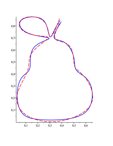
(a)

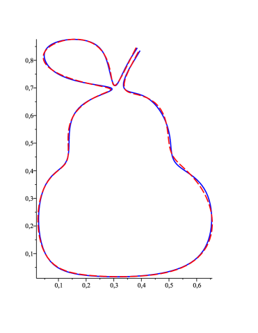
(b)

Figure 1: The original B-spline curve ,,Pear‘‘ of degree $5$ which is associated with the knot vector (5.3) (blue solid line), the B-spline curves of degree $5$ which are associated with the knot vectors (a) (5.4) and (b) (5.5), and computed in the process of knots removal (red dashed lines).

Next, let us apply the procedure of degree reduction to the B-spline curve ,,Pear‘‘. The resulting optimal B-spline curve of degree $3$ (errors: $E_{2}=2.76e{-}3$, $E_{\infty}=3.41e{-}2$) is shown in Figure 2a. The inner knots of this degree reduced curve are the same as in (5.3). The optimal B-spline curve of degree $4$ (errors: $E_{2}=4.64e{-}3$, $E_{\infty}=1.55e{-}2$) which is associated with the knot vector

$$K\setminus\left\{\frac{4}{20},\frac{13}{20},\frac{16}{20}\right\}$$ (5.6)

is illustrated in Figure 2b. This curve is a result of simultaneous degree reduction and knots removal.

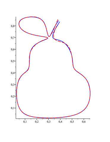
(a)

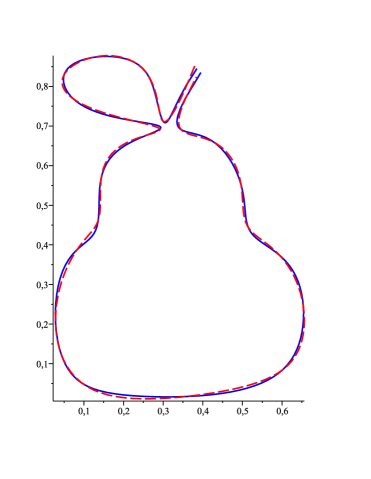
(b)

Figure 2: The original B-spline curve ,,Pear‘‘ of degree $5$ which is associated with the knot vector (5.3) (blue solid line), (a) the B-spline curve of degree $3$ which is associated with the knot vector having the same inner knots as in (5.3), and computed in the process of degree reduction (red dashed line), (b) the B-spline curve of degree $4$ which is associated with the knot vector (5.6), and computed in the process of simultaneous degree reduction and knots removal (red dashed line).

References

• [1] G. E. Andrews, R. Askey, R. Roy, Special functions, Cambridge University Press, Cambridge, 1999.
• [2] M. Bartoň, B. Jüttler, Computing roots of polynomials by quadratic clipping, Computer Aided Geometric Design 24 (2007), 125–141.
• [3] M. Bhatti, P. Bracken, The calculation of integrals involving B-splines by means of recursion relations, Applied Mathematics and Computation 172 (2006), 91–100.
• [4] J. Chen, G.-j. Wang, Approximate merging of B-spline curves and surfaces, Applied Mathematics-A Journal of Chinese Universities 25 (2010), 429–436.
• [5] Z. Ciesielski, The basis of B-splines in the space of algebraic polynomials, Ukrainian Mathematical Journal 38 (1987), 311–315.
• [6] E. Cohen, T. Lyche, R. Riesenfeld, Discrete B-splines and subdivision techniques in Computer-Aided Geometric Design and Computer Graphics, Computer Graphics and Image Processing 14 (1980), 87–111.
• [7] G. Dahlquist, Å. Björck, Numerical methods in scientific computing, volume I, SIAM, Philadelphia, 2008.
• [8] M. Eck, J. Hadenfeld, Knot removal for B-spline curves, Computer Aided Geometric Design 12 (1995), 259–282.
• [9] M. Flickner, J. Hafner, E. J. Rodriguez, J. L. C. Sanz, Periodic quasi-orthogonal spline bases and applications to least-squares curve fitting of digital images, IEEE Transactions on Image Processing 5 (1996), 71–88.
• [10] P. Gospodarczyk, S. Lewanowicz, P. Woźny, $G^{k,l}$-constrained multi-degree reduction of Bézier curves, Numerical Algorithms 71 (2016), 121–137.
• [11] P. Gospodarczyk, S. Lewanowicz, P. Woźny, Degree reduction of composite Bézier curves, Applied Mathematics and Computation 293 (2017), 40–48.
• [12] P. Gospodarczyk, P. Woźny, Efficient degree reduction of Bézier curves with box constraints using dual bases, preprint, 2016. Available at http://arxiv.org/abs/1511.08264.
• [13] J. Hoschek, Approximate conversion of spline curves, Computer Aided Geometric Design 4 (1987), 59–66.
• [14] B. Jüttler, The dual basis functions for the Bernstein polynomials, Advances in Computational Mathematics 8 (1998), 345–352.
• [15] M. Kamada, K. Toraichi, R. Mori, Periodic spline orthonormal bases, Journal of Approximation Theory 55 (1988), 27–34.
• [16] S. N. Kersey, Dual basis functions in subspaces of inner product spaces, Applied Mathematics and Computation 219 (2013), 10012–10024.
• [17] B.-G. Lee, Y. Park, Degree reduction of B-spline curves, Korean Journal of Computational and Applied Mathematics 8 (2001), 595–603.
• [18] S. Lewanowicz, P. Woźny, Dual generalized Bernstein basis, Journal of Approximation Theory 138 (2006), 129–150.
• [19] S. Lewanowicz, P. Woźny, P. Keller, Polynomial approximation of rational Bézier curves with constraints, Numerical Algorithms 59 (2012), 607–622.
• [20] L. Liu, L. Zhang, B. Lin, G. Wang, Fast approach for computing roots of polynomials using cubic clipping, Computer Aided Geometric Design 26 (2009), 547–559.
• [21] T. Lyche, K. Mørken, Knot removal for parametric B-spline curves and surfaces, Computer Aided Geometric Design 4 (1987), 217–230.
• [22] J. C. Mason, G. Rodriguez, S. Seatzu, Orthogonal splines based on B-splines – with applications to least squares, smoothing and regularisation problems, Numerical Algorithms 5 (1993), 25–40.
• [23] R.-j. Pan, B. Weng, Least Squares Degree Reduction of B-spline Curves, Journal of Chinese Computer Systems, 2009–02.
• [24] L. Piegl, W. Tiller, Algorithm for degree reduction of B-spline curves, Computer-Aided Design 27 (1995), 101–110.
• [25] L. Piegl, W. Tiller, The NURBS Book, second edition, Springer, Berlin, 1997.
• [26] H. Prautzsch, W. Boehm, M. Paluszny, Bézier and B-spline techniques, Springer, Berlin, 2002.
• [27] A. Redd, A comment on the orthogonalization of B-spline basis functions and their derivatives, Statistics and Computing 22 (2012), 251–257.
• [28] P. Sablonnière, Positive spline operators and orthogonal splines, Journal of Approximation Theory 52 (1988), 28–42.
• [29] I. J. Schoenberg, Notes on spline functions V. Orthogonal or Legendre splines, Journal of Approximation Theory 13 (1975), 84–104.
• [30] C.-L. Tai, S.-M. Hu, Q.-X. Huang, Approximate merging of B-spline curves via knot adjustment and constrained optimization, Computer-Aided Design 35 (2003), 893–899.
• [31] A. H. Vermeulen, R. H. Bartels, G. R. Heppler, Integrating products of B-splines, SIAM Journal on Scientific and Statistical Computing 13 (1992), 1025–1038.
• [32] Y. Wei, G. Wang, P. Yang, Legendre-like orthogonal basis for spline space, Computer-Aided Design 45 (2013), 85–92.
• [33] H. J. Wolters, G. Wu, G. Farin, Degree Reduction of B-Spline Curves, Computing Supplement 13 (1998), 235–241.
• [34] P. Woźny, Construction of dual bases, Journal of Computational and Applied Mathematics 245 (2013), 75–85.
• [35] P. Woźny, Construction of dual B-spline functions, Journal of Computational and Applied Mathematics 260 (2014), 301–311.
• [36] P. Woźny, P. Gospodarczyk, S. Lewanowicz, Efficient merging of multiple segments of Bézier curves, Applied Mathematics and Computation 268 (2015), 354–363.
• [37] P. Woźny, S. Lewanowicz, Multi-degree reduction of Bézier curves with constraints, using dual Bernstein basis polynomials, Computer Aided Geometric Design 26 (2009), 566–579.
• [38] J.-H. Yong, S.-M. Hu, J.-G. Sun, X.-Y. Tan, Degree reduction of B-spline curves, Computer Aided Geometric Design 18 (2001), 117–127.