Can a quantum critical state represent a blackbody?

Abstract

The blackbody theory of Planck played a seminal role in the development of quantum theory at the turn of the past century. A blackbody cavity is generally thought to be a collection of photons in thermal equilibrium; the radiation emitted is at all wavelengths, and the intensity follows a scaling law, which is Planck’s characteristic distribution law. These photons arise from non-interacting normal modes. Here we suggest that certain quantum critical states when heated emit “radiation” at all wavelengths and satisfy all the criteria of a blackbody. An important difference is that the “radiation” does not necessarily consist of non-interacting photons, but also emergent relativistic bosons or fermions. The examples we provide include emergent relativistic fermions at a topological quantum critical point. This perspective on a quantum critical state may be illuminating in many unforeseen ways.

I Introduction

A significant discovery of Planck was the fundamental constant of Nature, $h$ ($\hbar=h/2\pi$), which bears his name. The blackbody distribution of photons has survived significant tests in nature, although the idea of quantum discreteness of energy has a more complex history. Kuhn (1987) Two most important observations were a scaling law and the consistency with the Stefan-Boltmann law. Today we consider a black hole as a blackbody emitting Hawking radiation. In fact, it is also strongly argued, and experimentally determined from the cosmic microwave background, that the universe is a nearly perfect blackbody bathed in a radiation at a temperature of 2.7 $K$.

One might like to raise the question as to if there are other instances of blackbody radiation that may be interesting to study. We give several examples of such a possibility in condensed matter systems involving quantum critical points (QCP) and show how scale and conformal invariance play an important role in this matter. At the very outset we would like to dispel a possible misunderstanding. First, when we say radiation from a quantum critical point, we mean radiation from a state of matter tuned to a quantum critical point, not radiation from a single point in the phase space. Second, massless relativistic fermions can equally well provide a bonafide example of blackbody “radiation” (from hereon we shall omit the quotation mark, unless there is any possible confusion). However, what we have here are emergent relativistic fermions at topological quantum critical points tuned by the chemical potential, Goswami and Chakravarty (2011, 2016) not simply ad hoc non-interacting theories of free fermions.

More ambitious questions regarding what can perhaps be termed as interacting non-fermi liquid QCPs are reserved for the future. This is a thorny question: what appears to be strongly interacting Hamiltonian, under some clever choices of degrees of freedom, may represent noninteracting degrees of freedom. An example is an Ising model in a transverse field (TFIM) in $(1+1)$-dimensions, which by Jordan-Wigner transformation can be cast into a spinless free fermion theory with zero chemical potential at the QCP, separating a quantum disordered state from a spontaneously broken ferromagnetic state. Pfeuty (1970) These fermions are nonlocal in character, however. On the other hand, in the original spin variables TFIM is a strongly interacting problem with anomalous scaling dimensions. In the same spirit, we only consider those systems that can be transformed to noninteracting systems, however strongly interacting the original Hamiltonian may be. It should be kept in mind that there is a QCP separating two states of matter, and is thus not a trivial problem by any means.

Two important aspects of Planck’s theory are worth focusing on. The first is the Stefan-Boltzmann law and the second is a scaling function that forms the basis of Wien’s displacement law. The first states that the energy density of radiation, $u\propto T^{d+1}$ in $d$-dimensions; more generally $u\propto T^{\frac{d}{z}+1}$ to be discussed later, where $z$ is the dynamical critical exponent reflecting the anisotropy of scaling of time and space; the amplitude can contain additional physics (such as the central charge in a conformal field theory). The second is the phenomenology of the Wien’s law. In three spatial dimensions, the energy density per unit wavelength, $u_{\lambda}$, is

$$u_{\lambda}=\frac{c^{4}}{\lambda^{5}}F(\frac{c}{\lambda T}),$$ (1)

where $c$ is the velocity of light and $\lambda$ is the wavelength of radiation, and we have set the Planck and Boltzmann constants to unity. Here $F$ is a scaling function. In electrodynamic theory of non-interacting photons the frequency is uniquely related by $\omega=ck$. For later reference, let us rewrite it as

$$u_{\lambda}=\frac{T^{4}}{\lambda}G(\frac{c}{\lambda T}),$$ (2)

where $G(\frac{c}{\lambda T})=(\frac{c}{\lambda T})^{4}F(\frac{c}{\lambda T})$ is another scaling function with the same argument. The radiation exists at all all length scales satisfying the scaling law.

II What is a quantum critical point?

In this section we will provide a lightning summary of quantum critical points, at least those aspects of it that are relevant for the present discussion. Quantum criticality is a concept pertinent to zero temperature ($T=0$). Hertz (1976) A tuning parameter can drive a complex many-body system to a point $g_{c}$ (a generic coupling constant for the time being), where quantum fluctuations exist at all length scales, from the lattice scale to the correlation length $\xi=\infty$. But we cannot directly observe these remarkable fluctuations, because all experiments are necessarily carried out at a non-zero $T$. It is only through its influence on finite temperature observables that we can infer this phenomenon. Chakravarty et al. (1988); *Chakravarty:1989 There are now very good arguments and experiments that show that when tuned to $g_{c}$, the quantum criticality can extend to temperatures as large as the dominant fundamental energy scale of the Hamiltonian. Kopp and Chakravarty (2005); Kinross et al. (2014)

Similar to blackbody radiation we can define a scaling function (spectral function) at $T\neq 0$ by

$$A(k,\omega,g,T)=L_{\tau}^{y_{A}}A(kL_{\tau}^{1/z},\omega L_{\tau},L_{\tau}/\xi_{\tau})$$ (3)

where $\omega$ the frequency, and $k$ the wave vector, are two independent variables and are not necessarily tied to each other, as in the case of a photons; $y_{A}=d_{A}z$, $d_{A}$ is the scaling dimension of the operator $A$. The important scales are $L_{\tau}=\hbar/k_{B}T$ and the correlation timescale in imaginary time, $\tau$, given by $\xi_{\tau}\sim\xi^{z}$. The spatial correlation length $\xi\sim(|g-g_{c}|/g_{c})^{-\nu}$. Thus, $\xi_{\tau}^{1/z}$ defines the spatial length scale $\xi$. Here $z$, $\nu$ and $y_{A}$ are three independent exponents.

At $T=0$, a bit of care is needed to define the dynamic scaling function,

$$A(k,\omega,g)=\xi^{y_{A}}A(k\xi,\omega\xi_{\tau}).$$ (4)

However, when tuned exactly to $g_{c}$, the quantum critical point at $T=0$

$$A(k,\omega,g_{c})=k^{-y_{A}}A(k^{z}/\omega).$$ (5)

This is because at $T=0$ both $\xi_{\tau}$ and $\xi$ are infinite, so the only frequency scale left is $k^{z}\sim\omega$.

Let us now return to $T\neq 0$ but tuned to the $T=0$ quantum critical point $g_{c}$. Then a simple rearrangement leads to

$$A(k,\omega,g_{c},T)=\left({\frac{1}{T}}\right)^{y_{A}}\widetilde{A}\left(\frac{k^{z}}{T},\frac{\omega}{T}\right),$$ (6)

where we have set $\hbar=k_{B}=1$. This is the most general form of the displacement law. If we set $z=1$, with slight abuse of notation we can write,

$$A(k,\omega,g_{c},T)=\left({\frac{1}{T}}\right)^{y_{A}}\widetilde{A}\left(\frac{vk}{T}\right),$$ (7)

where $\omega=vk$, $v$ is an excitation velocity, which will be made more explicit on a case by case basis.

In the simplest possible scenario of a quantum critical point at $T=0$, there is one relevant parameter $g$ such that for $g>g_{c}$ the system flows to an attractive fixed point, defining a phase of matter with zero correlation length (well, almost), as we coarse grain the system, while for $g<g_{c}$, it flows to another phase. At the repulsive fixed point $g=g_{c}$, there are no flows and the correlation length is infinity, scale invariant. There are fluctuations on all length scales and time scales as discussed above. This flow is defined in the language of a differential equation in terms a dimensionless length scale:

$$\frac{dg}{d\ln\ell}=\beta({g}),$$ (8)

thus defining the renormalization group $\beta$-function.

III Conformal and scale invariance

QCPs are described by scale invariant quantum field theories. In essentially all known cases of physical relevance, QCPs with dynamical critical exponent $z=1$ have a traceless stress tensor, implying that scale invariance is promoted to conformal invariance, Francesco et al. (1997) and we assume this in mostly what follows. Scale invariance alone permits the trace of the stress tensor to be equal to the divergence of a local operator, while conformal invariance requires a strictly vanishing trace. In one spatial dimension the former implies the latter, while proving this in higher dimensions remains an outstanding problem. See Ref. Nakayama, 2015 for a review. For $z\neq 1$ tracelessness of the stress tensor is replaced by a more general relation discussed in the Appendix.

Let us consider a theory in the vicinity of a QCP, as described by the action $S=S_{\rm QCP}+\int d^{d}x\sum_{i}g_{i}{\cal O}_{i}$, and for the moment consider simply $z=1$. Then the stress tensor obeys the trace relation

$$T^{\mu}_{\mu}=\sum_{i}\Delta_{i}g_{i}{\cal O}_{i},$$ (9)

Here $\Delta_{i}=d_{i}+\gamma_{i}$ is the scaling dimension of ${\cal O}_{i}$, expressed in terms of the “engineering dimension” $d_{i}$ and the anomalous dimension $\gamma_{i}$ . A common case is where one has a classically scale invariant theory, so all $d_{i}$ vanish. We then usually write $\beta_{i}=\frac{dg_{i}}{d\ln\ell}=\gamma_{i}g_{i}$ and so

$$T_{\mu}^{\mu}=\sum_{i}\beta_{i}(g_{i}){\cal O}_{i}$$ (10)

For simplicity, if we consider only one operator ${\cal O}$, we have a remarkable identity

$$T_{\mu}^{\mu}=\beta({g}){\cal O}$$ (11)

This formula can be used in both directions: conformal invariance implies $T_{\mu}^{\mu}=0$ and so does the vanishing of $\beta(g)$ at the quantum critical point at $g=g_{c}$ at $T=0$. Cardy (2010)

If we confine ourselves to $g_{c}$ and increase the temperature, we can apply thermodynamic arguments to deduce the famous Stefan-Boltzmann law in any dimension up to a constant that cannot be deduced from thermodynamics alone. The calculation is well-known and elementary. We assume that the radiation emitted leads to a pressure $T_{\mu}^{\mu}=P-u/d=0$, where $u$ is the energy density. Because $T$ is traceless, when tuned to $g_{c}$ in $d$-dimensional space of volume $V=L^{d}$, the total energy $E=uV$ will obey the thermodynamic relation,

$$\left(\frac{\partial E}{\partial V}\right)_{T}=T\left(\frac{\partial P}{\partial T}\right)_{V}-P$$ (12)

It immediately follows that

$$(d+1)\frac{dT}{T}=\frac{du}{u},$$ (13)

hence

$$u\propto T^{d+1}$$ (14)

which is the Stefan-Boltzmann law. The proportionality constant hides crucially important physics, which is where the central charge enters. This is energy density not the power emitted and thus non-vanishing even in one dimension.

IV Transverse field Ising model as a nontrivial example

At a quantum critical point fluctuations of appropriate degrees of freedom diverge. However, what constitutes appropriate degrees of freedom is an interesting question. We will try to elaborate on this question by an explicit and simple (or not so simple) example of the one-dimensional transverse field Ising model (with a beautiful experimental realization Kinross et al. (2014)), whose connection with the blackbody radiation can be illustrated.

The Hamiltonian of TFIM is

$${\cal H}=-h\sum_{i}\sigma_{i}^{x}-J\sum_{i}\sigma_{i}^{z}\sigma_{i+1}^{z},$$ (15)

where the $\sigma$’s are the conventional Pauli matrices. An exact result is that the critical point is at $\lambda=h/J=1$. For $\lambda>1$ the system is quantum disordered, a paramagnet at $T=0$, and for $\lambda<1$ it is a ferromagnet with spontaneously broken $\mathbb{Z_{2}}$ symmetry. The phase diagram is shown in Fig. 1.

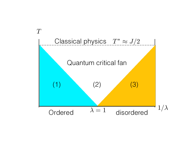
Figure 1: Phase diagram for TFIM. The region $(3)$ is the quantum disordered state, $(2)$ is the quantum critical regime, and (1) is the renormalized classical regime in the terminology of Chakravarty, Halperin and Nelson. Chakravarty et al. (1988); *Chakravarty:1989 The temperature $T^{*}=J/2$ determines the scale up to which quantum criticality effectively persists. Kopp and Chakravarty (2005)

By the well-known Jordan-Wigner transformation Pfeuty (1970), this Hamiltonian can be diagonalized in terms of free (but non-local) spin-less fermions, as

$${\cal H}=\sum_{k}\varepsilon_{k}\left(c^{\dagger}_{k}c_{k}-\frac{1}{2}\right),$$ (16)

where

$$\varepsilon_{k}=2J\left(1+\lambda^{2}-2\lambda\cos k\right)^{1/2};$$ (17)

when linearized around the quantum critical point the dispersion relation at large wavelengths is

$$\varepsilon_{k}\approx 2J\sqrt{2}\left|\sin\frac{k}{2}\right|\approx\sqrt{2}J|k|$$ (18)

The energy density at low temperature $T$ is then to the leading approximation

$$u_{F} \approx \frac{1}{2\pi}\int_{-\infty}^{\infty}dk\frac{\hbar v|k|}{e^{\hbar v|k|/k_{B}T}+1}$$ (19)

$$= \frac{\pi}{12}\frac{T^{2}}{\hbar v}=\frac{c\pi}{6\hbar v}T^{2}$$

where the velocity $v=\sqrt{2}J$, and buried in this expression is the central charge $c=1/2$ for spinless fermions. We can repeat the same calculation for free relativistic bosons. Then,

$$u_{B}=\frac{\pi}{6}\frac{T^{2}}{\hbar v_{B}},$$ (20)

where $v_{B}$ is the velocity of bosons. The central charge for bosons is unity. In either case one cannot tell what the degrees of freedom are without scrutinizing carefully the prefactor.

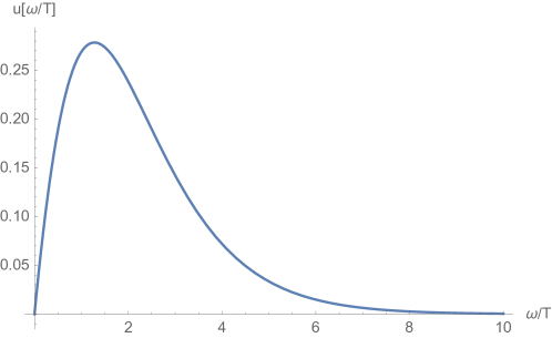
Figure 2: Energy density for Jordan-Wigner fermions for TFIM, $\omega=vk$,

The Wien displacement law follows trivially. Nowhere does the anomalous dimension of the respective fermion or boson operators enter. One could equally well deduce the results for the temperature dependence from thermodynamics.

In terms of the original spin variables, Jordan-Wigner fermions are non-local objects, as is well known:

$$c_{i} = \left(\prod_{j<i}\sigma_{j}^{z}\right)\sigma_{i}^{+},$$ (21)

$$c_{i}^{\dagger} = \left(\prod_{j<i}\sigma_{j}^{z}\right)\sigma_{i}^{-}.$$ (22)

The inverse is also non-local.

$$\sigma_{i}^{+} = \prod_{j<i}(1-2c_{j}^{\dagger}c_{j})c_{i},$$ (23)

$$\sigma_{i}^{-} = \prod_{j<i}(1-2c_{j}^{\dagger}c_{j})c_{i}^{\dagger}.$$ (24)

We do not see how one can locally couple to a single Jordan-Wigner fermion; so direct verification of the blackbody spectrum is probably not possible. On the other hand, the correlation function of $\sigma_{z}$ can be measured in neutron scattering from the frequency and momentum dependent susceptibility $\chi(k,\omega)$, which when tuned to criticality is Schulz (1986)

$$\chi(k,\omega)\propto\frac{1}{T^{7/4}}\frac{\Gamma(\frac{1}{16}-i\frac{\omega+vk}{4\pi T})\Gamma(\frac{1}{16}-i\frac{\omega-vk}{4\pi T})}{\Gamma(\frac{15}{16}-i\frac{\omega+vk}{4\pi T})\Gamma(\frac{15}{16}-i\frac{\omega-vk}{4\pi T})}$$ (25)

The imaginary part of $\chi(k,\omega)$ gives the fluctuation spectra shown in Fig. 3. One can clearly extract the characteristic velocity $v$, which is simply related to the exchange constant in TFIM.

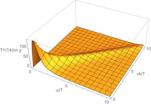
Figure 3: Imaginary part of the spin suceptibility for TFIM

V Higher Dimensional Models

We now provide examples of two higher dimensional models, where the QCP is controlled by massless Dirac fermions. Given the recently demonstrated idea of superuniversality, one can provide many more examples, Goswami and Chakravarty (2016) but we hope that these will suffice to make our point.

V.1 (2+1)-dimensions

First consider the low energy Hamiltonian of spinless fermions in two dimensions Read and Green (2000) with the spinor $\Psi_{k}^{\dagger}=(c_{k}^{*},c_{-k}$):

$$H=\frac{1}{2}\int\frac{d^{2}k}{(2\pi)^{2}}\;\Psi^{\dagger}_{\mathbf{k}}\widehat{{\cal H}}_{\mathbf{k}}\Psi_{\mathbf{k}},$$ (26)

where

$$\widehat{{\cal H}}_{k}=\hbar v(k_{x}\sigma_{x}+k_{y}\sigma_{y})+(-\mu+\hbar^{2}k^{2}/2m^{*})\sigma_{z}.$$ (27)

Here $\sigma_{x}$, $\sigma_{y}$, and $\sigma_{z}$ are the conventional Pauli matrices. Dirac fermions have a momentum dependent mass $m_{\mathbf{k}}=-\mu+\hbar^{2}k^{2}/(2m^{\ast})$ with $\mu$ being the chemical potential; the excitation velocity $v=\Delta_{t}/\sqrt{2m^{\ast}|\mu|}$ with $\Delta_{t}$ the triplet pairing amplitude. The energy dispersion is

$$E_{k}=\pm\sqrt{\hbar^{2}v^{2}k^{2}+m_{k}^{2}},$$ (28)

and the Hamiltonian can be brought to the form

$${\cal H}_{k}=|E_{k}|\hat{n}\cdot\hat{\sigma}.$$ (29)

The unit vector $\hat{n}$ is

$$\left(\frac{\hbar vk_{x}}{|E_{k}|},\frac{\hbar vk_{y}}{|E_{k}|},\frac{m_{k}}{|E_{k}|}\right)$$ (30)

At $k=0$,

$$\hat{n}=\left(0,0,\frac{-\mu}{|\mu|}\right)$$ (31)

and at $k\to\infty$

$$\hat{n}=\left(0,0,1\right).$$ (32)

Therefore, when $\mu>0$, there is a skyrmion with wrapping number unity in the BCS (Bardeen-Cooper-Schrieffer) phase. This corresponds to homotopy $\Pi^{2}(S^{2})=\mathbb{Z}$. On the other hand for $\mu<0$, the BEC (Bose-Einstein Condensation) phase does not admit skyrmions. Consequently, the topological distinction between the BEC and BCS states arises through the sign of the uniform Dirac mass or the chemical potential of the normal quasiparticles. Note that time reversal symmetry is broken and at QCP ($\mu=0$) the excitations are simply massless Dirac fermions in the low energy limit. Consequently, one is led to a simple blackbody radiation as the temperature is turned on. The physical context could be $p_{x}+ip_{y}$ superconductivity in $\mathrm{SrRu_{2}O_{4}}$. Kallin and Berlinsky (2016) Note that this is an emergent low energy Hamiltonian, where superconductivity is described in terms of Bogoliubov-de Gennes theory. The massless Dirac spectrum emerges only when the system is tuned to the quantum critical point at $\mu=0$. The derivation of the properties of the blackbody is a simple exercise.

How about interactions and/or disorder effects? In a sense interactions are already present in forming the superconducting state, for example, a large negative $U$ Hubbard model to form the diatomic molecule picture of BEC. However, additional short range interactions and mass disorder could also be added at the quantum critical point. The four fermion interaction has the scaling dimension $(z-d)=-1$ and is therefore irrelevant. Similarly the scaling dimension of disorder is $(2z-d)=0$, which is marginal, but is actually known to be marginally irrelevant. Evers and Mirlin (2008) Therefore, as long as we are aimed at the quantum critical point, the fermionic excitations remain valid and all the characteristics of blackbody radiation are satisfied.

V.2 $(3+1)$-dimensions

An analogous problem in the context of superfluid $\mathrm{{}^{3}He}$-B phase is given by the following low energy Hamiltonian Goswami and Chakravarty (2016)

$$H=\frac{1}{2}\int\frac{d^{3}k}{(2\pi)^{3}}\;\Psi^{\dagger}_{\mathbf{k}}\widehat{{\cal H}}(\mathbf{k})\Psi_{\mathbf{k}},$$ (33)

where $\Psi^{\dagger}_{\mathbf{k}}=(c^{\ast}_{\mathbf{k},\uparrow},c^{\ast}_{\mathbf{k},\downarrow},c_{-\mathbf{k},\uparrow},c_{-\mathbf{k},\downarrow})$ is the four component Nambu spinor, and $c_{\mathbf{k},s}$ is the annihilation operator for a normal state quasiparticle or fermionic ³He atom with spin projection $s=\uparrow/\downarrow$. The operator $\widehat{{\cal H}}(\mathbf{k})=\sum_{j=1}^{4}\;n_{j}(\mathbf{k})\Gamma_{j}$, where we have introduced a four component vector

$$\mathbf{n}(\mathbf{k})=(\hbar vk_{x},\hbar vk_{y},\hbar vk_{z},-\mu+\hbar^{2}k^{2}/(2m^{\ast})),$$ (34)

with $\mu$ and $m^{\ast}$ respectively being the chemical potential and the effective mass of the normal quasiparticles. The velocity $v=\Delta_{t}/(\hbar k_{F})=\Delta_{t}/\sqrt{2m^{\ast}|\mu|}$ with $\Delta_{t}$ being the triplet pairing amplitude, and $\Gamma_{j}$ are four mutually anticommuting Dirac matrices: $\Gamma_{1}=-\sigma_{3}\otimes\tau_{1}$, $\Gamma_{2}=-\sigma_{0}\otimes\tau_{2}$, $\Gamma_{3}=\sigma_{1}\otimes\tau_{1}$, $\Gamma_{4}=\sigma_{0}\otimes\tau_{3}$. The Pauli matrices $\sigma_{\mu}$ and $\tau_{\mu}$ respectively operate on the spin and particle-hole indices. By squaring the Hamiltonian one can bring it to the form

$$\widehat{{\cal H}}=|E_{k}|\hat{n}\cdot\vec{\Gamma}$$ (35)

where $\vec{\Gamma}$ is a four component vector composed of Dirac matrices defined above, and $\hat{n}$ now is a 4-component unit vector. Here $E_{k}=\pm\sqrt{\hbar^{2}v^{2}k^{2}+m_{k}^{2}}$, $k^{2}=k_{x}^{2}+k_{y}^{2}+k_{z}^{2}$ and $m_{\mathbf{k}}=-\mu+\hbar^{2}k^{2}/(2m^{\ast})$. Once again, at $k=0$,

$$\hat{n}=\left(0,0,0,\frac{-\mu}{|\mu|}\right)$$ (36)

and at $k\to\infty$

$$\hat{n}=\left(0,0,0,1\right).$$ (37)

It is again an example of a topological quantum criticality determined by the sign of $\mu$, leading to excitations consisting of $(3+1)$-dimensional Dirac fermions. The skyrmion number is given by the standard expression

$${\cal N}_{sk}=\frac{1}{12\pi^{2}}\epsilon_{ijk}\epsilon_{abcd}\int d^{3}k\;n_{a}\partial_{i}n_{b}\partial_{j}n_{c}\partial_{k}n_{d},$$ (38)

corresponding to the homotopy $\Pi_{3}(S^{3})=\mathbb{Z}$. Consequently, one is led to a simple blackbody radiation as the temperature is turned on, but now the time reversal invariance is respected. As before, additional short range interaction and mass disorder could also be added at the quantum critical point. A four fermion interaction has the scaling dimension $(z-d)=-2$ and is therefore irrelevant. Similarly the scaling dimension of disorder is $(2z-d)=-1$, which is also irrelevant. Therefore, as long as we are aimed at the quantum critical point, the characteristics of blackbody radiation are satisfied.

V.3 Discussion

So far we have considered examples where the dynamical exponent $z=1$. When $z\neq 1$, we must think anew. We interpret the generalized scaling function $A$ to be the imaginary part of the retarded Green function, i.e.,

$$A(k,\omega,g_{c},T)=\left({\frac{1}{T}}\right)^{y_{A}}\widetilde{A}\left(\frac{k^{z}}{T},\frac{\omega}{T}\right),$$ (39)

The anisotropic stress-energy tensor still satisfies an analogue of tracelessness and is proportional to the $\beta$-function as shown in the Appendix A. Thus, all the general characteristics of a blackbody are satisfied with minor modifications, for example, the Stefan-Boltzman law is modified to $u\propto T^{\frac{d}{z}+1}$ (See also Ref. Abrahams and W lfle, 2012).

There is a great deal of interest in non-Fermi liquids in condensed matter physics. They are mostly defined by power laws in transport coefficients, and these do not follow the Fermi liquid predictions. A famous example is the linear resistivity in high temperature superconductors, as a function of temperature, that extends over a wide range. But most importantly, non-Fermi liquids do not have quasiparticle poles in the spectral function but cuts. Yin and Chakravarty (1996) This, most likely, could lead to differences with conventional blackbody spectra. The other difference is that the spectra will contain substantial inhomogeneities due to the lack of a quasiparticle description; the inhomogeneity in the cosmic microwave background has been measured, but it is very small. This topic will be discussed in the future. On the other hand, we cannot see how this could possibly change the robust thermodynamic properties when tuned to the QCP, as mentioned earlier.

Unfortunately, the Jordan-Wigner fermions discussed earlier are highly non-local objects and cannot be measured by a local probe. On the other hand, if we could interpret them as the critical fermions at the BCS (Bardeen-Cooper-Schrieffer) to BEC (bose-Einstein Condensation) phase transition for a one-dimensional $p$-wave superconducting chain (which is an approximation in this case), they could be detected by a tunneling experiment. By contrast, consider the imaginary part of the spin susceptibility, as shown in Fig. 3, which reflects a strongly interacting system. The distinction between the two is quite striking. In terms of Jordan-Wigner fermions, the behavior is identical to that of a black body, peaking at an intermediate temperature for a given frequency. The maximum shifts as in Wien’s displacement law. On the other hand the spin susceptibility diverges at low frequencies, see Fig. 3. as it must since $g$ is tuned to the quantum critical point $g_{c}$. The quantum critical behavior of TFIM has been beautifully detected in NMR experiments in weakly coupled Ising spin chains, known as Cobalt Niobate ($\mathrm{CoNb_{2}O_{6}}$). Kinross et al. (2014) It is also possible to measure the fluctuation spectrum in neutron scattering measurements.

Although non-Fermi liquids are implicated in a large number of materials, such as cuprate high temperature superconductors, heavy fermions, etc., the universality of the behavior calls for a more fundamental understanding; the material dependence is of secondary importance. It is perhaps this goal that the present work may inspire. Of course, if the specific heat at low temperature is measured and neutron scattering experiments measure the characteristic excitation velocity, one can experimentally determine the central charge. It is of course possible to tune away from $g_{c}$, but we wanted to present our work in the simplest possible case. Of course, most of our results are well known; we simply provided a new perspective to view them.

Appendix A Trace of the stress tensor

Here we review the relation between scale invariance and the trace of the stress tensor, including the case of anistropic scaling, $z\neq 1$. See, for example, Ref. Baggio et al., 2012.

A.1 Isotropic scaling: $z=1$

We consider a general quantum field theory described by an action $S[\phi]$, and the corresponding path integral $Z=\int\!D\phi e^{-S[\phi]}$. The theory at the critical point is assumed to have dynamical scaling exponent $z=1$, and lives on the flat Euclidean metric $g_{\mu\nu}=\delta_{\mu\nu}$. We study the vicinity of the QCP by writing $S=S_{\rm QCP}+\int\sqrt{g}\sum_{i}g_{i}O_{i}$, where the operators $O_{i}$ have definite scaling dimensions at the QCP. Let the coupling $g_{i}$ have classical mass dimension $d_{i}$. Quantum mechanically we have to introduce an arbitrary renormalization scale $\mu$, and the couplings and operators depend on this scale. The renormalized path integral is written as $Z[g_{\mu\nu},g_{i}(\mu),\mu]$. Basic dimensional analysis tells us

$$Z[e^{2\sigma}g_{\mu\nu},e^{-d_{i}\sigma}g_{i}(\mu),e^{-\sigma}\mu]=Z[g_{\mu\nu},g_{i}(\mu),\mu]$$ (40)

Since the path integral doesn’t depend on $\mu$ we have

$$Z[e^{2\sigma}g_{\mu\nu},e^{-d_{i}\sigma}g_{i}(\mu),e^{-\sigma}\mu]=Z[e^{2\sigma}g_{\mu\nu},e^{-d_{i}\sigma}g_{i}(e^{\sigma}\mu),\mu]$$ (41)

and by definition of the anomalous dimension $\gamma_{i}$,

$$g_{i}(e^{\sigma}\mu)=e^{-\gamma_{i}\sigma}g_{i}(\mu)$$ (42)

The quantum statement of behavior under scale transformations is then

$$Z[e^{2\sigma}g_{\mu\nu},e^{-\Delta_{i}\sigma}g_{i},\mu]=Z[g_{\mu\nu},g_{i}(\mu),\mu]$$ (43)

where $\Delta_{i}=d_{i}+\gamma_{i}$ is the full scaling dimension. This implies the relation

$$2g_{\mu\nu}{\partial\ln Z\over\partial g_{\mu\nu}}=\sum_{i}\Delta_{i}g_{i}{\partial\ln Z\over\partial g_{i}}$$ (44)

We recall that the stress tensor is obtained by varying the metric,

$$\langle T_{\mu\nu}\rangle=-{2\over\sqrt{g}}{\delta\ln Z\over\delta g_{\mu\nu}}$$ (45)

and so the trace is

$$\langle T^{\mu}_{\mu}\rangle=-{2\over\sqrt{g}}g_{\mu\nu}{\delta\ln Z\over\delta g_{\mu\nu}}$$ (46)

Similarly, local operators insertions are obtained by varying the couplings,

$$\langle O_{i}\rangle=-{1\over\sqrt{g}}{\delta\ln Z\over\delta g_{i}}$$ (47)

Combining these results, we arrive at the operator relation

$$T^{\mu}_{\mu}=\sum_{i}\Delta_{i}g_{i}O_{i}$$ (48)

up to total derivatives (whose possible presence is related to the possible existence of scale but not conformally invariant theories.)

A common case is where one has a classically scale invariant theory, so all $d_{i}$ vanish. We then usually write $\beta_{i}=\mu{dg_{i}\over d\mu}=-\gamma_{i}g_{i}$ and so

$$T^{\mu}_{\mu}=-\sum_{i}\beta_{i}O_{i}$$ (49)

In the above we phrased the argument in terms of the renormalized path integral. Alternatively, from a more standard condensed matter viewpoint one might instead work with an explicit UV cutoff $\Lambda$. An analogous argument goes through.

A.2 Anisotropic scaling: $z\neq 1$

It’s useful to think of the theory as being defined on a metric of the form

$$ds^{2}=N^{2}dt^{2}+h_{ij}dx^{i}dx^{j}$$ (50)

with a preferred time foliation. For example, we can consider the following action with anisotropic scale invariance

$$S=\int\!dtd^{d-1}xN\sqrt{h}\left({1\over 2}N^{-2}(\partial_{t}\phi)^{2}-{1\over 2}\phi(\nabla^{i}\nabla_{i})^{z}\phi\right)$$ (51)

Here $\nabla_{i}$ denotes the covariant derivative built out of $h_{ij}$. For $z=1$ the action is Lorentz invariant (assuming constant $N$ and $h_{ij}$), but not otherwise.

Let us first discuss the classical theory. We focus on scale transformations,

$$h_{ij}\to e^{2\sigma}h_{ij}~{},\quad N\to e^{z\sigma}N~{},\quad\phi\to e^{{z+1-d\over 2}\sigma}\phi$$ (52)

under which the action is invariant. When the equations of motion are satisfied the action is stationary, ${\delta S\over\delta\phi}=0$, and then we have

$$2h_{ij}{\delta S\over\delta h_{ij}}+zN{\delta S\over\delta N}=0$$ (53)

We define the energy density $\cal E$ and spatial stress tensor (momentum flux) $\Pi^{ij}$ as

$${\cal E}={1\over\sqrt{h}}{\delta S\over\delta N}~{},\quad\Pi^{ij}={2\over N\sqrt{h}}{\delta S\over\delta h_{ij}}$$ (54)

so that that

$$z{\cal E}+\Pi^{i}_{i}=0$$ (55)

which is the generalization of $T^{\mu}_{\mu}=0$ to theories with $z\neq 1$.

Turning to the quantum theory, we consider a scale invariant theory with path integral

$$Z[N,h_{ij}]=\int\!D\phi e^{-S}$$ (56)

which obeys

$$Z[e^{z\sigma}N,e^{2\sigma}h_{ij}]=Z[N,h_{ij}]$$ (57)

and so we have

$$\langle{\cal E}\rangle=-{1\over\sqrt{h}}{\delta\ln Z\over\delta N}~{},\quad\langle\Pi^{ij}\rangle=-{2\over N\sqrt{h}}{\delta\ln Z\over\delta h_{ij}}$$ (58)

This generalizes to include other operator insertions. The invariance in Eq. (57) implies the operator equation $z{\cal E}+\Pi^{i}_{i}=0$.

Now let’s add other operators to the action

$$S=S_{\rm QCP}+\int\!dtd^{d-1}xN\sqrt{h}\sum_{i}g_{i}O_{i}$$ (59)

The couplings $g_{i}$ are taken to have engineering dimension $d_{i}$, by which we mean that classically

$$Z[e^{z\sigma}N,e^{2\sigma}h_{ij},e^{-d_{i}\sigma}g_{i}]=Z[N,h_{ij},g_{i}]$$ (60)

We also note

$$\langle O_{i}\rangle=-{1\over N\sqrt{h}}{\delta\ln Z\over\delta g_{i}}$$ (61)

Now include quantum effects. We need to introduce an arbitrary renormalization scale $\mu$, and the couplings $g_{i}(\mu)$ depend on this scale, as do the operators. The previous scale transformation must be accompanied by a scaling of $\mu$,

$$Z[\lambda^{z}N,\lambda^{2}h_{ij},\lambda^{-d_{i}}g_{i}(\mu),\lambda^{-1}\mu]=Z[N,h_{ij},g_{i}(\mu),\mu]$$ (62)

On the other hand, the path integral is $\mu$ independent, so

$$Z[e^{z\sigma}N,e^{2\sigma}h_{ij},e^{-d_{i}\sigma}g_{i}(\mu),e^{-\sigma}\mu]=Z[e^{z\sigma}N,e^{2\sigma}h_{ij},e^{-d_{i}\sigma}g_{i}(\lambda\mu),\mu]$$ (63)

hence

$$Z[e^{z\sigma}N,e^{2\sigma}h_{ij},e^{-d_{i}\sigma}g_{i}(\lambda\mu),\mu]=Z[N,h_{ij},g_{i}(\mu),\mu]$$ (64)

Using the definition of the $\beta$ function

$$\mu{d\over d\mu}g_{i}(\mu)=\beta_{i}(g)$$ (65)

we find

$$zN{\delta\ln Z\over\delta N}+2h_{ij}{\delta\ln Z\over\delta h_{ij}}+(\beta_{i}-d_{i}g_{i}){\delta\ln Z\over\delta g_{i}}=0$$ (66)

which implies the operator equation

$$z{\cal E}+\Pi^{i}_{i}=\sum_{i}(d_{i}g_{i}O_{i}-\beta_{i}O_{i})$$ (67)

Classically marginal operators have $d_{i}=0$.

References

- Kuhn (1987) Thomas S. Kuhn, Blackbody theory and Quantum Discontibuity 1894-1912 (University of Chicago Press, 1987).
- Goswami and Chakravarty (2011) Pallab Goswami and Sudip Chakravarty, “Quantum criticality between topological and band insulators in dimensions,” Phys. Rev. Lett. 107, 196803 (2011).
- Goswami and Chakravarty (2016) Pallab Goswami and Sudip Chakravarty, “Superuniversality of topological quantum phase transition and global phase diagram of dirty topological systems in three dimensions,” arXiv:1603.03763 (2016).
- Pfeuty (1970) Pierre Pfeuty, “The one-dimensional ising model with a transverse field,” Annals of Physics 57, 79–90 (1970).
- Hertz (1976) John A. Hertz, “Quantum critical phenomena,” Phys. Rev. B 14, 1165–1184 (1976).
- Chakravarty et al. (1988) Sudip Chakravarty, Bertrand I. Halperin, and David R. Nelson, “Low-temperature behavior of two-dimensional quantum antiferromagnets,” Phys. Rev. Lett. 60, 1057–1060 (1988).
- Chakravarty et al. (1989) Sudip Chakravarty, Bertrand I. Halperin, and David R. Nelson, “Two-dimensional quantum Heisenberg antiferromagnet at low temperatures,” Phys. Rev. B 39, 2344–2371 (1989).
- Kopp and Chakravarty (2005) A. Kopp and S. Chakravarty, “Criticality in correlated quantum matter,” Nature Phys. 1, 53–56 (2005).
- Kinross et al. (2014) A. W. Kinross, M. Fu, T. J. Munsie, H. A. Dabkowska, G. M. Luke, Subir Sachdev, and T. Imai, “Evolution of quantum fluctuations near the quantum critical point of the transverse field ising chain system ,” Phys. Rev. X 4, 031008 (2014).
- Francesco et al. (1997) Philippe-Di Francesco, Pterre Mathieu, and David Senechal, Conformal Field theory (Springer-Verlag, New York, 1997).
- Nakayama (2015) Yu Nakayama, “Scale invariance vs conformal invariance,” Phys. Rept. 569, 1–93 (2015), arXiv:1302.0884 [hep-th] .
- Cardy (2010) John Cardy, “The ubiquitous ’ c ’: from the Stefan– Boltzmann law to quantum information,” Journal of Statistical Mechanics: Theory and Experiment 2010, P10004 (2010).
- Schulz (1986) H. J. Schulz, “Phase diagrams and correlation exponents for quantum spin chains of arbitrary spin quantum number,” Phys. Rev. B 34, 6372–6385 (1986).
- Read and Green (2000) N. Read and Dmitry Green, “Paired states of fermions in two dimensions with breaking of parity and time-reversal symmetries and the fractional quantum hall effect,” Phys. Rev. B 61, 10267–10297 (2000).
- Kallin and Berlinsky (2016) Catherine Kallin and John Berlinsky, “Chiral superconductors,” Reports on Progress in Physics 79, 054502 (2016).
- Evers and Mirlin (2008) Ferdinand Evers and Alexander D. Mirlin, “Anderson transitions,” Rev. Mod. Phys. 80, 1355–1417 (2008).
- Abrahams and W lfle (2012) Elihu Abrahams and Peter W lfle, “Critical quasiparticle theory applied to heavy fermion metals near an antiferromagnetic quantum phase transition,” Proceedings of the National Academy of Sciences 109, 3238–3242 (2012).
- Yin and Chakravarty (1996) Lan Yin and Sudip Chakravarty, “Spectral anomaly and high temperature superconductors,” Int. J. of Mod. Phys, B 10, 805–845 (1996).
- Baggio et al. (2012) Marco Baggio, Jan de Boer, and Kristian Holsheimer, “Anomalous Breaking of Anisotropic Scaling Symmetry in the Quantum Lifshitz Model,” JHEP 07, 099 (2012), arXiv:1112.6416 [hep-th] .