Structure and computation of two-dimensional incompressible extended MHD

Abstract

A comprehensive study of a reduced version of Lüst’s equations, the extended magnetohydrodynamic (XMHD) model obtained from the two-fluid theory for electrons and ions with the enforcement of quasineutrality, is given. Starting from the Hamiltonian structure of the fully three-dimensional theory, a Hamiltonian two-dimensional incompressible four-field model is derived. In this way energy conservation along with four families of Casimir invariants are naturally obtained. The construction facilitates various limits leading to the Hamiltonian forms of Hall, inertial, and ideal MHD, with their conserved energies and Casimir invariants. Basic linear theory of the four-field model is treated, and the growth rate for collisionless reconnection is obtained. Results from nonlinear simulations of collisionless tearing are presented and interpreted using, in particular normal fields, a product of the Hamiltonian theory that gives rise to simplified equations of motion.

I Introduction

Out of necessity for practicable computation, for many decades researchers have produced reduced fluid models for describing aspects of laboratory and naturally occurring plasmas. Applications of such models include the exploration of MHD kink modes by means of reduced MHD,rmhd subsequently extended to include, among other effects, Hall and gyro physics HKM85 as well as parallel compressibility and diamagnetic effects.DA84 Further applications range from the investigation of drift-waves HW83 to low-frequency turbulence Bri92 ; Dor93 ; Sny01 ; SSB05 and magnetic reconnection. SPK94 ; GCPP01 ; Grasso07 ; TMWG08 ; WHM09 ; Sco10 ; Wae12 ; KWM15

The various models have been obtained by various means: in some cases rigorous asymptotics were employed, while other models were built on intuition, or using the device of effecting closure by constraining to match a desired linear theory (e.g. Ref. HKM85, ). Based on the noncanonical Hamiltonian formalism introduced for MHD in Ref. MG80, (see e.g.  Refs. M98, ; M05, for review) it was advocated in a series of papersMH84 ; MM84 ; HHM86 ; Haz87 that retention of Hamiltonian form can serve as a derivational aide or as a filter for selecting out good theories in the ideal limit. By ideal limit, is meant the limit of the model where all dissipative terms, such as collisions, Landau damping, and dissipative anomalous transport terms are neglected. Subsequently there have been many papers by many authors that have adopted this point of view.

In the present work we consider the two-dimensional (2D) incompressible reduction of the XMHD model derived by Lüst in Ref. Lust, . This model is simply a reduced case of a two-fluid model in which the charge quasineutrality condition is invoked, the displacement current is ignored, and the smallness of the electron-ion mass ratio is taken to the first order approximation. The value of the XMHD model resides in its ability to capture and describe the main two-fluid effects, e.g., Hall drift and electron inertia. Unlike its parent 3D version, Abd15 ; Lin15 the 2D incompressible reduction of XMHD (RXMHD) has not yet been explored, however, from the above mentioned Hamiltonian perspective. The Hamiltonian approach can indeed be particularly fruitful in this context because of the richness of the Casimir invariants that typically emerge in 2D models. These invariants, which are associated with the Hamiltonian structure, provide information on the dynamics. Identifying the Hamiltonian structure of RXMHD and providing its Casimir invariants is one of the goals of this paper. A further related issue that we treat, is that of investigating how the conservation laws related to the Casimir invariants in RXMHD, which properly accounts for both ion and electron physics corrections, compare with those of submodels such as ideal reduced, Hall and inertial MHD, where some of these effects are neglected.

In addition to the investigation of the Hamiltonian structure of the model, we also present an application of RXMHD where the Hamiltonian approach plays a role. Given that RXMHD is a model that extends 2D incompressible Hall MHD by properly accounting for electron physics, a natural application for RXMHD is to 2D magnetic reconnection driven by electron inertia. Such magnetic reconnection has already been studied by means of a model very similar to RXMHD in Ref. Bis97, . These authors considered a weakly dissipative model and identified the fundamental mechanisms of two-fluid collisionless reconnection, in particular with regard to the role of the Hall term and of the electron MHD governing the dynamics at scales below the ion skin depth. In the present manuscript we carry out an investigation of purely non-dissipative magnetic reconnection by means of RXMHD, with an approach that is somewhat complementary to that adopted in Ref. Bis97, . We provide an analytical expression for the linear growth rate of reconnecting perturbations and check it against numerical solutions, and we take advantage of the Hamiltonian formulation to compare the evolution of the physical fields, in terms of which the model was originally formulated, with normal fields, an alternative set of variables. Normal fields are associated with the Casimir invariants and express a simpler dynamics. This approach was used in previous studies of collisionless reconnection in Hamiltonian models (see, e.g.  Refs. GCPP01, ; Del06, ; Gra09, ; Tas10, ; Com12, ). Also, the Hamiltonian formulation provides the correct expression for the total energy, which we exploit in order to investigate the redistribution of magnetic energy into different forms. We also remark that, in a recent publication,And14 a model very similar to RXMHD was adopted to investigate numerical reconnection rates and the conservation of three invariants during reconnection.

Our paper is organized as follows. In Sec. II, XMHD is reviewed and the Hamiltonian form of RXMHD, a four-field model, is obtained from that of the full model.Abd15 ; Lin15 Consequences of this reduction are explored in Sec. III where it is shown that in addition to the energy, the RXMHD system posses four infinite families of invariants, the Casimir invariants. In addition, the so-called normal fields are obtained and it is observed that the equations of motion take a particularly simple form when expressed in terms of them (compare Eqs. (25)-(28) to Eqs. (50)-(51)). Section  IV treats various limits of RXMHD leading to reduced Hall MHD (RHMHD), reduced inertial MHD (RIMHD) and reduced MHD (RMHD). Numerical solution of RXMHD is treated in Sec. V. Here the dispersion relation is plotted for the basic modes of the system, the collisionless tearing instability growth rate is identified and numerically verified, and nonlinear simulations of collisionless tearing are performed, which reveal how energy migrates from field into flow. Finally, in Sec. VI we summarize our results and draw conclusions.

II Derivation Of reduced extended magnetohydrodynamics

II.1 Extended magnetohydrodynamics

The governing equations of extended magnetohydrodynamics (XMHD) are the continuity equation

$$\frac{\partial\rho}{\partial t}=-\nabla\cdot\left(\rho\mathbf{V}\right),$$ (1)

the force law,

$$\rho\left(\frac{\partial\mathbf{V}}{\partial t}+\left(\mathbf{V}.\nabla\right)\mathbf{V}\right) = -\nabla p+\mathbf{J}\times\mathbf{B}$$ (2)

$$-d^{2}_{e}\left(\mathbf{J}\cdot\nabla\right)\frac{\mathbf{J}}{\rho},$$

and the generalized Ohm’s law

$$\mathbf{E}+\mathbf{V}\times\mathbf{B} = -\frac{d_{i}}{\rho}\nabla p_{e}+d_{i}\frac{\mathbf{J}}{\rho}\times\mathbf{B}$$ (3)

$$+d^{2}_{e}\left[\frac{\partial}{\partial t}\left(\frac{\mathbf{J}}{\rho}\right)+(\mathbf{V}\cdot\nabla)\frac{\mathbf{J}}{\rho}+\left(\frac{\mathbf{J}}{\rho}\cdot\nabla\right)\mathbf{V}\right]$$

$$-d_{i}d^{2}_{e}\left(\frac{\mathbf{J}}{\rho}\cdot\nabla\right)\frac{\mathbf{J}}{\rho}.$$

Here $\rho$ is the total mass density, $\mathbf{V}$ is the center of mass velocity, $\mathbf{B}$ is the magnetic field, $\mathbf{E}$ is the electric field, $\mathbf{J}$ is the current density and $p=p_{i}+p_{e}$ is the total pressure, with $p_{i}$ being the ion pressure and $p_{e}$ the electron pressure. The system is normalized to the standard Alfvénic units with $d_{e}=c/(\omega_{pe}L)$ and $d_{i}=c/(\omega_{pi}L)$, corresponding to the normalized electron and ion skin depths, respectively, where $\omega_{pe}$ and $\omega_{pi}$ are the electron and ion plasma frequencies, and $L$ is the system size. Equations (1)–(3) are coupled with the pre-Maxwell equations

$$\nabla\times\mathbf{E}=-\frac{\partial\mathbf{B}}{\partial t}\qquad\textrm{and}\qquad\nabla\times\mathbf{B}=\mathbf{J},$$ (4)

and for this paper the systems will be closed by assuming a barotropic equation of state, i.e., the pressure $p$ is assumed to depend only on the density $\rho$.

Upon using $\rho^{-1}\nabla p=\nabla h\left(\rho\right)$, which follows from the barotropic assumption, where $h\left(\rho\right)$ is the enthalpy, and using the pre-Maxwell equations (4), one can obtain, from Eqs. (2) and (3), the following system:

$$\frac{\partial\mathbf{V}}{\partial t} = -\left(\nabla\times\mathbf{V}\right)\times\mathbf{V}+\rho^{-1}\left(\nabla\times\mathbf{B}\right)\times\mathbf{B}^{\ast}$$ (5)

$$\leavevmode\nobreak\ \leavevmode\nobreak\ \leavevmode\nobreak\ \leavevmode\nobreak\ -\nabla\left(h+V^{2}/2+d^{2}_{e}\left(\nabla\times\mathbf{B}\right)^{2}/2\rho^{2}\right),$$

$$\frac{\partial\bm{B}^{\ast}}{\partial t} = \nabla\times\left(\mathbf{V}\times\mathbf{B}^{\ast}\right)-\nabla\times\left(\rho^{-1}\left(\nabla\times\mathbf{B}\right)\times\mathbf{B}^{\ast}\right)$$ (6)

$$\leavevmode\nobreak\ \leavevmode\nobreak\ \leavevmode\nobreak\ \leavevmode\nobreak\ +d^{2}_{e}\nabla\times\left(\rho^{-1}\left(\nabla\times\mathbf{B}\right)\times\left(\nabla\times\mathbf{V}\right)\right),$$

where

$$\mathbf{B}^{\ast} = \mathbf{B}+d^{2}_{e}\nabla\times\rho^{-1}\left(\nabla\times\mathbf{B}\right).$$ (7)

Equations (1), (5) and (6) with the total energy,Kimura14

$$\mathscr{H}:=\int d^{3}x\left\{\rho\left(\frac{V^{2}}{2}+U\left(\rho\right)\right)+\frac{\mathbf{B}\cdot\mathbf{B}^{\ast}}{2}\right\},$$ (8)

as Hamiltonian, and the Poisson bracket

$$\left\{F,G\right\} = -\int d^{3}x\leavevmode\nobreak\ \bigg{\{}\left[F_{\rho}\nabla\cdot G_{\mathbf{V}}+F_{\mathbf{V}}\cdot\nabla G_{\rho}\right]$$

$$-\left[\frac{\left(\nabla\times\mathbf{V}\right)}{\rho}\cdot\big{(}F_{\mathbf{V}}\times G_{\mathbf{V}}\big{)}\right]$$

$$-\left[\frac{\mathbf{B}^{\ast}}{\rho}\cdot\big{(}F_{\mathbf{V}}\times\left(\nabla\times G_{\mathbf{B}^{\ast}}\right)\big{)}\right]$$

$$-\left[\frac{\mathbf{B}^{\ast}}{\rho}\cdot\big{(}\left(\nabla\times F_{\mathbf{B}^{\ast}}\right)\times G_{\mathbf{V}}\big{)}\right]$$

$$+d_{i}\left[\frac{\mathbf{B}^{\ast}}{\rho}\cdot\big{(}\left(\nabla\times F_{\mathbf{B}^{\ast}}\right)\times\left(\nabla\times G_{\mathbf{B}^{\ast}}\right)\big{)}\right]$$

$$-d^{2}_{e}\left[\frac{\left(\nabla\times\mathbf{V}\right)}{\rho}\cdot\big{(}\left(\nabla\times F_{\mathbf{B}^{\ast}}\right)\times\left(\nabla\times G_{\mathbf{B}^{\ast}}\right)\big{)}\right]\bigg{\}}$$

constitute a noncanonical Hamiltonian system in which the phase space is spanned by the dynamical variables $\rho,\mathbf{V}$, and $\mathbf{B}^{\ast}$. In (II.1) $F_{\bm{\xi}}:=\delta F/\delta\bm{\xi}$ denote the functional derivative of the functional $F$ with respect to the dynamical variable $\bm{\xi}$. The full Poisson bracket of Eq. (II.1) and a proof of the Jacobi identity were first given in Ref. Abd15, , with further properties and a simplified proof of the Jacobi identity given in Ref. Lin15, . The bracket of Eq. (II.1) is an extension of the MHD bracket first given in Ref. MG80, , amended by the inclusion of two additional terms, one proportional to $d_{i}$, accounting for the Hall effect, and one proportional to $d_{e}^{2}$, accounting for electron inertia.

The Poisson bracket (II.1) has three independent Casimir invariants,

$$\mathcal{C}_{1} = \int d^{3}x\leavevmode\nobreak\ \mathbf{B}^{\ast}\cdot\left(\mathbf{V}-\frac{d_{i}}{2d^{2}_{e}}\mathbf{A}^{\ast}\right),$$ (10)

$$\mathcal{C}_{2} = \int d^{3}x\leavevmode\nobreak\ \left[\mathbf{B}^{\ast}\cdot\mathbf{A}^{\ast}+d^{2}_{e}\mathbf{V}\cdot\left(\nabla\times\mathbf{V}\right)\right],$$ (11)

$$\mathcal{C}_{3} = \int d^{3}x\leavevmode\nobreak\ \rho.$$ (12)

Combining $\mathcal{C}_{1}$ and $\mathcal{C}_{2}$, produces the “canonical helicities”

$$\mathcal{C}_{\pm}=\frac{1}{2}\int d^{3}x\leavevmode\nobreak\ \mathbf{P}^{\pm}\cdot\left(\nabla\times\mathbf{P}^{\pm}\right),$$ (13)

where $\mathbf{P}^{\pm}=\mathbf{V}+\lambda_{\pm}\mathbf{A}^{\ast},$ with

$$\lambda_{\pm}=\frac{-d_{i}\pm\sqrt{d^{2}_{i}+4d^{2}_{e}}}{2d^{2}_{e}}.$$ (14)

II.2 Reduced extended MHD

II.2.1 Direct reduction

In the incompressible limit, the reduced extended magnetohydrodynamics (RXMHD) can be obtained by writing $\mathbf{V}$ and $\mathbf{B}$ in the Clebsch-like forms

$$\mathbf{B}\left(x,y,t\right) = \nabla\psi\left(x,y,t\right)\times\widehat{z}+b\left(x,y,t\right)\widehat{z},$$ (15)

$$\mathbf{V}\left(x,y,t\right) = -\nabla\phi\left(x,y,t\right)\times\widehat{z}+v\left(x,y,t\right)\widehat{z}\,,$$ (16)

where $\psi$ and $\phi$ are the flux and stream functions, respectively, and $b$ and $v$ are $\widehat{z}$-components of these fields. From (15), the current density $\mathbf{J}$ is seen to be given by

$$\mathbf{J}=\nabla\times\mathbf{B}=\nabla b\times\widehat{z}-\nabla^{2}\psi\,\widehat{z},$$ (17)

Upon setting $\rho=1$ and using (15) and (16), the $\widehat{z}$-component of Eq. (2) yields

$$\frac{\partial v}{\partial t} = -\left[\phi,v\right]+\left[b,\psi\right]-d^{2}_{e}\left[b,\nabla^{2}\psi\right],$$ (18)

where $\left[f,g\right]=\nabla f\times\nabla g\cdot\widehat{z}$, is the standard canonical Poisson bracket with $x$ and $y$ as canonically conjugate coordinates. Similarly, operating with $\widehat{z}\cdot\nabla\times$ on (2) yields

$$\frac{\partial\nabla^{2}\phi}{\partial t} = -\left[\phi,\nabla^{2}\phi\right]-\left[\nabla^{2}\psi,\psi\right]-d^{2}_{e}\left[b,\nabla^{2}b\right]\,,$$ (19)

and the $\hat{z}$-component of (3) is

$$-\frac{\partial\psi}{\partial t}+\left[\psi,\phi\right] = d_{i}\left[b,\psi\right]-d^{2}_{e}\frac{\partial}{\partial t}\nabla^{2}\psi+d^{2}_{e}\left[\nabla^{2}\psi,\phi\right]$$ (20)

$$+d^{2}_{e}\left[v,b\right]-d_{i}d^{2}_{e}\left[b,\nabla^{2}\psi\right],$$

where we made use of the relation $E_{z}=-\partial\psi/\partial t$. Finally operating with $\widehat{z}\cdot\nabla\times$ on (3) gives

$$-\frac{\partial b}{\partial t} +\left[v,\psi\right]-\left[\phi,b\right]=d_{i}\left[\psi,\nabla^{2}\psi\right]-d^{2}_{e}\frac{\partial}{\partial t}\nabla^{2}b$$ (21)

$$+d^{2}_{e}\left[\nabla^{2}\phi,b\right]+d^{2}_{e}\left[\nabla^{2}b,\phi\right]-d_{i}d^{2}_{e}\left[b,\nabla^{2}b\right].$$

Therefore, with the definitions

$$\omega = \nabla^{2}\phi$$ (22)

$$\psi^{\ast} = \psi-d^{2}_{e}\nabla^{2}\psi$$ (23)

$$b^{\ast} = b-d^{2}_{e}\nabla^{2}b\,,$$ (24)

the RXMHD equations can be written as follows:

$$\frac{\partial\psi^{\ast}}{\partial t} = -\left[\phi,\psi^{\ast}\right]-d_{i}\left[b,\psi^{\ast}\right]+d^{2}_{e}\left[b,v\right],$$ (25)

$$\frac{\partial\omega}{\partial t} = -\left[\phi,\omega\right]-\left[\nabla^{2}\psi,\psi\right]-d^{2}_{e}\left[b,\nabla^{2}b\right],$$ (26)

$$\frac{\partial b^{\ast}}{\partial t} = -\left[\phi,b^{\ast}\right]+d_{i}\left[\nabla^{2}\psi,\psi\right]+\left[v,\psi\right]$$ (27)

$$\leavevmode\nobreak\ \leavevmode\nobreak\ \leavevmode\nobreak\ \leavevmode\nobreak\ \leavevmode\nobreak\ \leavevmode\nobreak\ \leavevmode\nobreak\ \leavevmode\nobreak\ \leavevmode\nobreak\ \leavevmode\nobreak\ +d^{2}_{e}\left[b,\omega\right]+d_{i}d^{2}_{e}\left[b,\nabla^{2}b\right],$$

$$\frac{\partial v}{\partial t} = -\left[\phi,v\right]+\left[b,\psi^{\ast}\right]\,.$$ (28)

The Hamiltonian (energy) (8) in terms of the new variables becomes

$$\mathscr{H}:=\frac{1}{2}\int d^{2}x\left(-\phi\omega-\nabla^{2}\psi\psi^{*}+bb^{*}+v^{2}\right)\,,$$ (29)

which can be shown by direct calculation to be conserved by the RXMHD system of (25)–(28).

II.2.2 Reduction via chain rule

Another way to obtain RXMHD is by Hamiltonian reduction. With this method the Poisson bracket (II.1) is rewritten in terms of the new variables via the functional chain rule (see e.g.  Refs. amp0, ; amp1, where this is done for MHD). This method has the advantage of yielding directly the Hamiltonian structure of RXMHD.

The chain rule proceeds by assuming functionals obtain their dependence on $\mathbf{V}$ and $\mathbf{B}^{\ast}$ through the new variables $\omega,v,\psi^{\ast}$, and $b^{\ast}$, i.e.

$$F\left[\mathbf{V},\mathbf{B}^{\ast}\right]=\bar{F}\left[\omega,v,\psi^{\ast},b^{\ast}\right]$$ (30)

Varying both sides of (30) gives

$$\int d^{2}x\leavevmode\nobreak\ F_{\mathbf{V}}\cdot\delta\mathbf{V}=\int d^{2}x\leavevmode\nobreak\ \Big{(}\bar{F}_{\omega}\,\delta\omega+\bar{F}_{v}\,\delta v\Big{)},$$ (31)

while variation of the velocity field $\mathbf{V}$ of (16) gives

$$\delta\mathbf{V}=\widehat{z}\times\nabla\delta\phi+\delta v\widehat{z}.$$ (32)

From (32) we obtain

$$\delta v=\widehat{z}\cdot\delta\mathbf{V}$$ (33)

while $\widehat{z}\times\delta\mathbf{V}=-\nabla\delta\phi$. Thus using $\delta\omega=\nabla\cdot\nabla\delta\phi$, we obtain

$$\delta\omega=\nabla\cdot\big{(}\delta\mathbf{V}\times\widehat{z}\big{)}\,.$$ (34)

Upon inserting Eqs. (32) and (34) into Eq. (31), performing an integration by parts, and using the arbitrariness of $\delta\mathbf{V}$ we obtain

$$F_{\mathbf{V}}=\nabla\bar{F}_{\omega}\times\hat{z}+\bar{F}_{v}.$$ (35)

In a similar way we obtain

$$\nabla\times F_{\mathbf{B}^{\ast}}=\nabla\bar{F}_{b^{\ast}}\times\hat{z}+\bar{F}_{\psi^{\ast}}\hat{z}.$$ (36)

Now we are in position to use (35) and (36) to reduce the Poisson bracket of (II.1) to one in terms of the reduced variables. This calculation gives

$$\{F,G\} = \int d^{2}x\bigg{\{}\psi^{\ast}\bigg{(}\left[F_{\omega},G_{\psi^{*}}\right]+\left[F_{\psi^{*}},G_{\omega}\right]$$

$$+ \left[F_{v},G_{b^{*}}\right]+\left[F_{b^{*}},G_{v}\right]$$

$$- d_{i}\left(\left[F_{\psi^{*}},G_{b^{*}}\right]+\left[F_{b^{*}},G_{\psi^{*}}\right]\right)\bigg{)}$$

$$+ \omega\Big{(}\left[F_{\omega},G_{\omega}\right]+d_{e}^{2}\left[F_{b^{*}},G_{b^{*}}\right]\Big{)}$$

$$+ b^{*}\Big{(}\left[F_{\omega},G_{b^{*}}\right]+\left[F_{b^{*}},G_{\omega}\right]-d_{i}\left[F_{b^{*}},G_{b^{*}}\right]\Big{)}$$

$$+ v\Big{(}\left[F_{\omega},G_{v}\right]+\left[F_{v},G_{\omega}\right]$$

$$+ d_{e}^{2}\big{(}\left[F_{\psi^{*}},G_{b^{*}}\right]+\left[F_{b^{*}},G_{\psi^{*}}\right]\big{)}\Big{)}\bigg{\}},$$

where, consistent with the representation (16), we have removed the $\rho$ dependence and used the relation

$$\int d^{2}x\leavevmode\nobreak\ f\left[g,h\right]=\int d^{2}x\leavevmode\nobreak\ h\left[f,g\right]=\int d^{2}x\leavevmode\nobreak\ g\left[h,f\right],$$ (38)

valid for generic functions $f$, $g$ and $h$ and appropriate boundary conditions. Here and henceforth, we drop the bars on the functionals.

The above bracket (II.2.2) with the Hamiltonian (29) produces the equations of motion (25)–(28) in the form $\partial\zeta/\partial t=\left\{\zeta,\mathscr{H}\right\}$, where $\zeta=\left(\psi^{\ast},\omega,b^{\ast},v\right)^{t}$ denotes the dynamical variables of the system.

II.3 Jacobi identity

As a further check that the set of equations (25)–(28) with the Hamiltonian (29) constitutes a noncanonical Hamiltonian system with Poisson bracket (II.2.2), we verify the following requisite bracket properties: antisymmetric

• antisymmetry

  $$\left\{F,G\right\}=-\left\{G,F\right\},$$

• Leibniz property

  $$\left\{FG,H\right\}=F\left\{G,H\right\}+G\left\{F,H\right\},$$

• Jacobi identity

  $$\left\{F,\left\{G,H\right\}\right\}+\left\{H,\left\{F,G\right\}\right\}+\left\{G,\left\{H,F\right\}\right\}=0,$$

Assuming boundary conditions such that surface terms vanishes, as would be the case for periodic boundary conditions, we can easily demonstrate the first two properties. However, the proof of Jacobi identity is more difficult. A direct proof is tedious, but instead we can follow the general theory of Ref. Thi00, . Using $\zeta=\left(\psi^{\ast},\omega,b^{\ast},v\right)^{t}$ with each field being indexed by $\zeta^{\mu}$, $\mu=1,\cdots,4$, we can write (II.2.2) in the form

$$\{F,G\}=\int d^{2}x[F_{\mu},F_{\nu}]W^{\mu\nu}_{\gamma}\zeta^{\gamma},$$ (39)

where $F_{\mu}=\delta F/\delta\zeta^{\mu}$ and the quantities $W^{\mu\nu}_{\gamma}$ are symmetric in their upper indices. Considering the $W^{\mu\nu}_{\gamma}$ as a family of matrices indexed by $\nu$, the Jacobi identity is satisfied if and only if the following matrices pairwise commute:

$$W^{(\omega)} = \begin{pmatrix}1&0&0&0&\\ 0&1&0&0&\\ 0&0&1&0&\\ 0&0&0&1&\end{pmatrix},W^{(\psi^{*})}=\begin{pmatrix}0&0&0&0&\\ 1&0&-d_{i}&0&\\ 0&0&0&0&\\ 0&0&d_{e}^{2}&0&\end{pmatrix},$$

$$W^{(b^{*})} = \begin{pmatrix}0&0&d_{e}^{2}&0&\\ 0&-d_{i}&0&1&\\ 1&0&-d_{i}&0&\\ 0&d_{e}^{2}&0&0&\end{pmatrix},W^{(v)}=\begin{pmatrix}0&0&0&0&\\ 0&0&1&0&\\ 0&0&0&0&\\ 1&0&0&0&\end{pmatrix},$$

which follows from a relatively easy calculation. Consequently, the Poisson bracket (II.2.2) satisfies the Jacobi identity.

II.4 Remarkable transformations

In Ref. Lin15, it was shown that the Poisson bracket (II.1) follows from a remarkable sequence of variable and parameter transformations of a basic bracket for Hall MHD. This led a dramatically simplified calculation for the Jacobi identity and quite naturally to the Casimir invariants. We will show that the reduced Poisson bracket of (II.2.2) possesses analogous transformations.

Specifically, the bracket (II.1) maps into the Poisson bracket of Hall MHD in terms of the field $\mathbf{B}_{\lambda_{\pm}}$, when one carries out the transformation

$$\mathbf{B}_{\lambda_{\pm}}=\mathbf{B}^{*}+\lambda_{\pm}^{-1}\nabla\times\mathbf{V},$$ (40)

The analogous transformation in our 2D case would then be of the form,

$$\mathbf{B}_{\lambda_{\pm}}=\nabla Phys.\leavevmode\nobreak\ Lett.\leavevmode\nobreak\ \times\hat{z}+b_{\lambda_{\pm}}\hat{z}$$ (41)

and this suggests the change of variables

$$Phys.\leavevmode\nobreak\ Lett.\leavevmode\nobreak\ =\psi^{*}+v/\lambda_{\pm},\qquad b_{\lambda_{\pm}}=b^{*}+\omega/\lambda_{\pm}.$$ (42)

With this change of variables, the bracket (II.2.2) becomes

$$\{F,G\} = \int\!\!d^{2}x\Bigg{\{}\psi_{\lambda_{\pm}}\!\bigg{(}\!\!\left(\frac{2}{\lambda_{\pm}}-d_{i}\right)\!\!\Big{(}\!\left[F_{\psi_{\lambda_{\pm}}},G_{b_{\lambda_{\pm}}}\right]$$

$$+ \left[F_{b_{\lambda_{\pm}}},G_{\psi_{\lambda_{\pm}}}\right]\Big{)}+\left[F_{\psi_{\lambda_{\pm}}},G_{\omega}\right]+\left[F_{\omega},G_{\psi_{\lambda_{\pm}}}\right]$$

$$+ \left[F_{v},G_{b_{\lambda_{\pm}}}\right]+\left[F_{b_{\lambda_{\pm}}},G_{v}\right]\bigg{)}+\omega\left[F_{\omega}G_{\omega}\right]$$

$$+ v\Big{(}\left[F_{\omega},G_{v}\right]+\left[F_{v},G_{\omega}\right]\Big{)}+b_{\lambda_{\pm}}\bigg{(}\left[F_{\omega},G_{b_{\lambda_{\pm}}}\right]$$

$$+ \left[F_{b_{\lambda_{\pm}}},G_{\omega}\right]+\left(\frac{2}{\lambda_{\pm}}-d_{i}\right)\left[F_{b_{\lambda_{\pm}}},G_{b_{\lambda_{\pm}}}\right]\bigg{)}\Bigg{\}}\,.$$

Note that one obtains the bracket (II.4) for either choice of the values of $\lambda_{\pm}$ in Eq. (14). Also, note that the bracket (II.4) is identical to the Poisson bracket identified by Eqs. (43)–(44) in Ref. Haz87, if one replaces, in the latter bracket, $\beta$ with $-1$ and $2\delta\beta$ with $2/\lambda_{\pm}-d_{i}$. We have thus shown that the bracket (II.2.2) can be transformed, by means of an invertible change of variables, into a known Poisson bracket for which the Jacobi identity has already been proven. Consequently, this serves as an alternative verification that the bracket (II.2.2) satisfies the Jacobi identity. We remark that the model in Ref. Haz87, (in the 2D cold ion limit with no magnetic curvature), is isomorphic to 2D incompressible Hall MHD, which is consistent with the above mentioned general result of Ref. Lin15, .

Given the relationship to the results of Ref. Haz87, we can immediately identify the Casimir invariants and normal fields, a special class of field variables, which we consider next.

III Normal fields and Casimir invariants

III.1 Normal fields

The four-field bracket of (II.4) is complicated, as one might expect considering the physics described by the RXMHD model. However, as described in Ref. Thi00, , noncanonical brackets can be mapped by coordinate changes into special simplified forms. For systems of four fields, there are only a few such simplified forms. The fields in which the bracket is simplified are called normal fields – for the present case they are given by

$$\begin{split}\psi_{+}=&Phys.\leavevmode\nobreak\ Lett.\leavevmode\nobreak\ ,\qquad\psi_{-}=Phys.\leavevmode\nobreak\ Lett.\leavevmode\nobreak\ -\left(\frac{2}{\lambda_{+}}-d_{i}\right)v,\\ b_{+}=&b_{\lambda_{\pm}},\qquad b_{-}=b_{\lambda_{\pm}}-\left(\frac{2}{\lambda_{+}}-d_{i}\right)\omega.\end{split}$$ (44)

In terms of these normal fields the bracket (II.4) becomes

$$\{F,G\} = \left(\frac{2}{\lambda_{+}}-d_{i}\right)\!\int\!\!d^{2}x\bigg{\{}\psi_{+}\Big{(}[F_{\psi_{+}},G_{b_{+}}]$$ (45)

$$+ [F_{b_{+}},G_{\psi_{+}}]\Big{)}+b_{+}[F_{b_{+}},G_{b_{+}}]-b_{-}[F_{b_{-}},G_{b_{-}}]$$

$$- \psi_{-}\Big{(}[F_{\psi_{-}},G_{b_{-}}]+[F_{b_{-}},G_{\psi_{-}}]\Big{)}\bigg{\}}\,,$$

a form that is the direct sum of two semidirect product brackets (see Ref. Thi00, ). In terms of the normal fields $\psi_{\pm},b_{\pm}$ the corresponding Casimirs for this bracket are known to be

$$C_{1,2}=\int d^{2}x\leavevmode\nobreak\ \mathcal{F}_{\pm}\left(\psi_{\pm}\right),\\ \leavevmode\nobreak\ \leavevmode\nobreak\ \leavevmode\nobreak\ \leavevmode\nobreak\ \leavevmode\nobreak\ \leavevmode\nobreak\ \leavevmode\nobreak\ C_{3,4}=\int d^{2}x\leavevmode\nobreak\ b_{\pm}\mathcal{G}_{\pm}\left(\psi_{\pm}\right),$$ (46)

with $\mathcal{F}_{\pm}$ and $\mathcal{G}_{\pm}$ arbitrary functions.

We remark that, in the 2D incompressible limit, the Casimir invariants $\mathcal{C}_{1,2}$ of XMHD reduce to

$$\int d^{2}x\leavevmode\nobreak\ \mathbf{B}^{\ast}\cdot\left(\mathbf{V}-\frac{d_{i}}{2d^{2}_{e}}\mathbf{A}^{\ast}\right)$$

$$=\int d^{2}x\left(\omega\psi^{\ast}+vb^{\ast}-\frac{d_{i}}{2d^{2}_{e}}\psi^{\ast}b^{\ast}\right),$$ (47)

and

$$\int d^{2}x\leavevmode\nobreak\ \big{[}\mathbf{B}^{\ast}\cdot\mathbf{A}^{\ast}+d^{2}_{e}\textbf{V}\cdot\left(\nabla\times\mathbf{V}\right)\big{]}$$

$$=\int d^{2}x\left(\psi^{\ast}b^{\ast}+d^{2}_{e}\,v\omega\right),$$ (48)

respectively. Such Casimir invariants indeed correspond to linear combinations of the Casimir invariants $C_{3,4}$ of Eq. (46), for the particular choice $\mathcal{G}_{\pm}=\psi_{\pm}$. This shows how the Casimir invariants of XMHD are related to those of RXMHD.

We remark that, in Ref. And14, , a system isomorphic to RXMHD was studied but only three out of the infinite number of invariants of the model were presented.

Noting that $2/\lambda_{+}-d_{i}=1/\lambda_{+}-1/\lambda_{-}$, we find that the normal fields are related to the original variables by

$$\psi_{\pm}=\psi^{*}+\frac{v}{\lambda_{\pm}}\qquad\mathrm{and}\qquad b_{\pm}=b^{*}+\frac{\omega}{\lambda_{\pm}}.$$ (49)

In terms of the normal fields the RXMHD system obtains the perspicuous form

$$\frac{\partial\psi_{\pm}}{\partial t}+\left[\phi_{\pm},\psi_{\pm}\right] = 0,$$ (50)

$$\frac{\partial b_{\pm}}{\partial t}+\left[\phi_{\pm},b_{\pm}\right] = \lambda_{\pm}[\psi_{\pm},\psi],$$ (51)

where $\phi_{\pm}=\phi-d_{e}^{2}\lambda_{\pm}b$. Here we also made use of the relation $d_{i}-1/\lambda_{\pm}=-d_{e}^{2}\lambda_{\pm}$. From Eqs. (50) and (51) it emerges that $\psi_{\pm}$ are Lagrangian invariants of the model, reminiscent of Ohm’s law for reduced MHD (RMHD), whereas the equations describing $b_{\pm}$ are reminiscent of the RMHD vorticity equation.

We remark that, by expanding in the limit $d_{e}^{2}/d_{i}^{2}\rightarrow 0$, one can obtain the following relations:

$$\psi_{+}\simeq\psi+d_{i}v_{iz},\qquad\psi_{-}\simeq\psi-\frac{d_{e}^{2}}{d_{i}}v_{ez},$$ (52)

$$\hat{z}\times\nabla\phi_{+}\simeq\mathbf{v}_{i\perp},\qquad\hat{z}\times\nabla\phi_{-}\simeq\mathbf{v}_{e\perp},$$ (53)

$$b_{+}\simeq b+d_{i}\omega_{i},\qquad b_{-}\simeq b-\frac{d_{e}^{2}}{d_{i}}\omega_{e},$$ (54)

$$\phi\simeq\phi_{+}+\frac{d_{e}^{2}}{d_{i}^{2}}\phi_{-},\qquad b\simeq\frac{\phi_{-}-\phi_{+}}{d_{i}},$$ (55)

where $v_{iz}$ and $v_{ez}$ are the $z$-components of the ion and electron fluid velocities, (so that $\nabla^{2}\psi=(v_{ez}-v_{iz})/d_{i}$ and $v\simeq v_{iz}+(d_{e}^{2}/d_{i}^{2})v_{ez})$, $\mathbf{v}_{i\perp}$ and $\mathbf{v}_{e\perp}$ are the ion and electron perpendicular fluid velocities, whereas $\omega_{i,e}=\hat{z}\cdot\nabla\times\mathbf{v}_{i,e\perp}$ are the $z$ components of the corresponding vorticities. From Eqs. (52)–(54) it emerges then that $\psi_{\pm}$ correspond to the $z$-components of the canonical momenta for ions and electrons. These are advected, according to Eqs. (50), by the perpendicular ion and electron velocities, respectively. The normal fields $b_{\pm}$, on the other hand, represent some generalized vorticities, analogous to the generalized vorticity of Hall-MHD.

The Hamiltonian (29) can be expressed in terms of the normal fields by making use of the following transformations:

$$\psi^{\ast}=\frac{\lambda_{+}\psi_{+}-\lambda_{-}\psi_{-}}{\lambda_{+}-\lambda_{-}},\qquad v=\frac{\psi_{+}-\psi_{-}}{d_{e}^{2}(\lambda_{+}-\lambda_{-})},$$ (56)

$$b^{*}=\frac{\lambda_{+}b_{+}-\lambda_{-}b_{-}}{\lambda_{+}-\lambda_{-}},\qquad\omega=\frac{b_{+}-b-}{d_{e}^{2}(\lambda_{+}-\lambda_{-})},$$ (57)

and introducing the linear operator $\mathcal{L}$, such that $\psi^{\ast}=\mathcal{L}\psi$ and $b^{*}=\mathcal{L}b$. Assuming this operator is invertible, one can then write

$$\psi=\mathcal{L}^{-1}\frac{\lambda_{+}\psi_{+}-\lambda_{-}\psi_{-}}{\lambda_{+}-\lambda_{-}},\quad b=\mathcal{L}^{-1}\frac{\lambda_{+}b_{+}-\lambda_{-}b_{-}}{\lambda_{+}-\lambda_{-}},$$ (58)

and replace these expressions in (29). The resulting functional is

$$\begin{split}\mathscr{H}=\frac{1}{2}\int d^{2}x&\bigg{(}-\frac{b_{+}-b{-}}{d_{e}^{2}\left(\lambda_{+}-\lambda_{-}\right)}\nabla^{-2}\frac{b_{+}-b{-}}{d_{e}^{2}\left(\lambda_{+}-\lambda_{-}\right)}\\ &+\frac{\lambda_{+}b_{+}-\lambda_{-}b_{-}}{\lambda_{+}-\lambda_{-}}\mathcal{L}^{-1}\frac{\lambda_{+}b_{+}-\lambda_{-}b_{-}}{\lambda_{+}-\lambda_{-}}\\ &-\frac{\lambda_{+}\psi_{+}-\lambda_{-}\psi_{-}}{\lambda_{+}-\lambda_{-}}\nabla^{2}\mathcal{L}^{-1}\frac{\lambda_{+}\psi_{+}-\lambda_{-}\psi_{-}}{\lambda_{+}-\lambda_{-}}\\ &+\frac{\psi_{+}^{2}-2\psi_{+}\psi_{-}+\psi_{-}^{2}}{d_{e}^{4}\left(\lambda_{+}-\lambda_{-}\right)^{2}}\bigg{)}.\end{split}$$ (59)

Because the Hamiltonian of (59) is complicated it may be more straightforward to consider that of (29) in terms of the original variables. An approximate form can be obtained by neglecting again $d_{e}^{2}/d_{i}^{2}$ when compared to terms of order unity, and making use of the relations (53), (55), and the relation $\nabla^{2}\psi=(v_{ez}-v_{iz})/d_{i}$. This leads to the following approximate expression for the Hamiltonian:

$$\mathscr{H} \simeq \frac{1}{2}\int d^{2}x\bigg{(}|\nabla\psi|^{2}+b^{2}+v_{i\perp}^{2}+v_{iz}^{2}$$ (60)

$$\hskip 56.9055pt+\frac{d_{e}^{2}}{d_{i}^{2}}\left(v_{e\perp}^{2}+v_{ez}^{2}\right)\bigg{)}.$$

The expression (60) shows that the Hamiltonian is nearly given by the sum of magnetic energy (the first two terms on the right-hand side of (60)), with the ion kinetic energy (third and fourth terms) and the electron kinetic energy (fifth and sixth terms).

IV Limits of RXMHD

IV.1 2D incompressible Hall MHD

If we set $d_{e}=0$ in Eqs. (25)–(28), we obtain the 2D incompressible Hall MHD system

$$\frac{\partial\psi}{\partial t} = -[\phi,\psi]-d_{i}[b,\psi],$$ (61)

$$\frac{\partial\omega}{\partial t} = -[\phi,\omega]-[\nabla^{2}\psi,\psi],$$ (62)

$$\frac{\partial b}{\partial t} = -[\phi,b]+d_{i}[\nabla^{2}\psi,\psi]+[v,\psi],$$ (63)

$$\frac{\partial v}{\partial t} = -[\phi,v]+[b,\psi].$$ (64)

As anticipated above, this model is also Hamiltonian, with Hamiltonian functional

$$H=\frac{1}{2}\int d^{2}x\left(|\nabla\phi|^{2}+|\nabla\psi|^{2}+b^{2}+v^{2}\right),$$ (65)

and Poisson bracket

$$\begin{split}\{F,G\}=&\int d^{2}x\bigg{\{}\psi\bigg{(}\left[F_{\omega},G_{\psi}\right]+\left[F_{\psi},G_{\omega}\right]+\left[F_{v},G_{b}\right]\\ &+\left[F_{b},G_{v}\right]-d_{i}\left(\left[F_{\psi},G_{b}\right]+\left[F_{b},G_{\psi^{*}}\right]\right)\bigg{)}\\ &+\omega\left[F_{\omega},G_{\omega}\right]+v\Big{(}\left[F_{\omega},G_{v}\right]+\left[F_{v},G_{\omega}\right]\Big{)}\\ &+b\Big{(}\left[F_{\omega},G_{b}\right]+\left[F_{b},G_{\omega}\right]-d_{i}\left[F_{b},G_{b}\right]\Big{)}\bigg{\}}.\end{split}$$ (66)

This system, which previously appeared in Ref. Haz87, , has the Casimirs

$$C_{1} = \int d^{2}x\leavevmode\nobreak\ \mathcal{K}\left(\psi\right),$$ (67)

$$C_{2} = \int d^{2}x\leavevmode\nobreak\ b\leavevmode\nobreak\ \mathcal{S}\left(\psi\right),$$ (68)

$$C_{3} = \int d^{2}x\leavevmode\nobreak\ \mathcal{T}\left(\psi_{H}\right),$$ (69)

$$C_{4} = \int d^{2}x\leavevmode\nobreak\ b_{H}\leavevmode\nobreak\ \mathcal{R}\left(\psi_{H}\right),$$ (70)

where $b_{H}=b+d_{i}\omega$, $\psi_{H}=\psi+d_{i}v$ and $\mathcal{K},\mathcal{S},\mathcal{T}$ and $\mathcal{R}$ are arbitrary functions. In particular, for $\mathcal{S}=\psi$ and $\mathcal{R}=\psi_{H}$ one retrieves the 2D incompressible versions of the functionals

$$\int d^{3}x\leavevmode\nobreak\ \mathbf{A}\cdot\mathbf{B},$$ (71)

and

$$\int d^{2}x\left(\mathbf{A}+d_{i}\mathbf{V}\right)\cdot\left(\mathbf{B}+d_{i}\nabla\times\mathbf{V}\right),$$ (72)

respectively, which are Casimir invariants for 3D Hall MHD, corresponding to magnetic helicity and to a generalized magnetic helicity.

IV.2 2D incompressible inertial MHD

If we set $d_{i}=0$ in Eqs. (25)–(28) while retaining $d_{e}$, we obtain the 2D incompressible inertial MHD system

$$\frac{\partial\psi^{\ast}}{\partial t} = -\left[\phi,\psi^{\ast}\right]+d^{2}_{e}\left[b,v\right],$$ (73)

$$\frac{\partial\omega}{\partial t} = -\left[\phi,\omega\right]-\left[\nabla^{2}\psi,\psi\right]-d^{2}_{e}\left[b,\nabla^{2}b\right],$$ (74)

$$\frac{\partial b^{\ast}}{\partial t} = -\left[\phi,b^{\ast}\right]+\left[v,\psi\right]+d^{2}_{e}\left[b,\omega\right],$$ (75)

$$\frac{\partial v}{\partial t} = -\left[\phi,v\right]+\left[b,\psi^{\ast}\right].$$ (76)

In this limit the Hamiltonian (29) does not change, but the Poisson brackets becomes

$$\begin{split}\{F,G\}=\int d^{2}x&\bigg{\{}\psi^{\ast}\bigg{(}\left[F_{\omega},G_{\psi^{*}}\right]+\left[F_{\psi^{*}},G_{\omega}\right]\\ &+\left[F_{v},G_{b^{*}}\right]+\left[F_{b^{*}},G_{v}\right]\bigg{)}\\ &+\omega\Big{(}\left[F_{\omega},G_{\omega}\right]+d_{e}^{2}\left[F_{b^{*}},G_{b^{*}}\right]\Big{)}\\ &+b^{*}\Big{(}\left[F_{\omega},G_{b^{*}}\right]+\left[F_{b^{*}},G_{\omega}\right]\Big{)}\\ &+v\Big{(}\left[F_{\omega},G_{v}\right]+\left[F_{v},G_{\omega}\right]\\ &+d_{e}^{2}\big{(}\left[F_{\psi^{*}},G_{b^{*}}\right]+\left[F_{b^{*}},G_{\psi^{*}}\right]\big{)}\Big{)}\bigg{\}}.\end{split}$$ (77)

We can easily proof that the above system is Hamiltonian through one of the methods discussed in Sec. II.3.

It may seem odd to retain $d_{e}$ while dropping $d_{i}$, since they scale with the mass ration, but this limit may make sense in a different ordering.Kimura14

The Poisson bracket (77) possesses the following four families of Casimir invariants:

$$C_{1,2} = \int d^{2}x\leavevmode\nobreak\ \mathcal{Y}_{\pm}\left(\psi^{i}_{\pm}\right),$$ (78)

$$C_{3,4} = \int d^{2}x\leavevmode\nobreak\ b^{i}_{\pm}\mathcal{P}_{\pm}\left(\psi^{i}_{\pm}\right),$$ (79)

where $b^{i}_{\pm}=b^{\ast}\pm d_{e}\omega,\psi^{i}_{\pm}=\psi^{\ast}\pm d_{e}v$ and $\mathcal{Y}_{\pm}$ and $\mathcal{P}_{\pm}$ are arbitrary functions.

3D inertial MHD, which previously appeared in Ref. Lin15, , has the Casimirs

$$\int d^{3}x\leavevmode\nobreak\ \mathbf{B}^{\ast}\cdot\mathbf{V}$$ (80)

and

$$\int d^{3}x\leavevmode\nobreak\ \big{[}\mathbf{B}^{\ast}\cdot\mathbf{A}^{\ast}+d^{2}_{e}\textbf{V}\cdot\left(\nabla\times\mathbf{V}\right)\big{]},$$ (81)

which, in their 2D incompressible limit, become

$$\int d^{2}x\,(\omega\psi^{*}+b^{*}v),$$ (82)

and

$$\int d^{2}x\,(\psi^{*}b^{*}+d_{e}^{2}v\leavevmode\nobreak\ \omega),$$ (83)

respectively. These are linear combinations of

$$\int d^{2}x\,b_{\pm}^{i}\psi_{\pm}^{i},$$ (84)

corresponding to the Casimir invariants $C_{3,4}$ of Eq. (79) for the choice $\mathcal{P}_{\pm}=\psi_{\pm}^{i}$.

IV.3 2D incompressible ideal MHD

The 2D incompressible ideal MHD system can be obtained by setting $d_{i}=d_{e}=0$ in Eqs. (25)–(28), giving

$$\frac{\partial\psi}{\partial t} = -\left[\phi,\psi\right],$$ (85)

$$\frac{\partial\omega}{\partial t} = -\left[\phi,\omega\right]-\left[\nabla^{2}\psi,\psi\right],$$ (86)

$$\frac{\partial b}{\partial t} = -\left[\phi,b\right]+\left[v,\psi\right],$$ (87)

$$\frac{\partial v}{\partial t} = -\left[\phi,v\right]+\left[b,\psi\right].$$ (88)

Reduced ideal MHD has energy

$$H=\frac{1}{2}\int d^{2}x\left(|\nabla\phi|^{2}+|\nabla\psi|^{2}+b^{2}+v^{2}\right)\,,$$ (89)

and the Poisson bracket

$$\begin{split}\{F,G\}=\int d^{2}x&\Big{\{}\psi\Big{(}\left[F_{\omega},G_{\psi}\right]+\left[F_{\psi},G_{\omega}\right]+\left[F_{v},G_{b}\right]\\ &+\left[F_{b},G_{v}\right]\Big{)}+\omega\left[F_{\omega},G_{\omega}\right]\\ &+v\Big{(}\left[F_{\omega},G_{v}\right]+\left[F_{v},G_{\omega}\right]\Big{)}\\ &+b\Big{(}\left[F_{\omega},G_{b}\right]+\left[F_{b},G_{\omega}\right]\Big{)}\Big{\}}.\end{split}$$ (90)

This reduced ideal MHD model, which previously appeared in Ref. Haz87, , has the Casimirs

$$C_{1} = \int d^{2}x\leavevmode\nobreak\ \mathcal{I}\left(\psi\right),$$ (91)

$$C_{2} = \int d^{2}x\leavevmode\nobreak\ b\leavevmode\nobreak\ \mathcal{O}\left(\psi\right),$$ (92)

$$C_{3} = \int d^{2}x\leavevmode\nobreak\ v\leavevmode\nobreak\ \mathcal{Q}(\psi),$$ (93)

$$C_{4} = \int d^{2}x\leavevmode\nobreak\ (\omega\leavevmode\nobreak\ \mathcal{U}(\psi)+b\leavevmode\nobreak\ v\leavevmode\nobreak\ \mathcal{U}^{\prime}(\psi)),$$ (94)

where $\mathcal{I},\mathcal{O},\mathcal{Q},\mathcal{U}$ are arbitrary functions and the prime symbol denotes derivative with respect to the argument of the function.

With the choices $\mathcal{O}=\psi$ and $\mathcal{U}=\psi$ one retrieves, from $C_{2}$ and $C_{4}$ in Eqs. (92) and (94), the 2D incompressible versions of the magnetic helicity

$$\int d^{3}x\leavevmode\nobreak\ \mathbf{A}\cdot\mathbf{B}$$ (95)

and of the cross-helicity

$$\int d^{3}x\leavevmode\nobreak\ \mathbf{V}\cdot\mathbf{B}$$ (96)

of 3D ideal MHD.

V Numerical results

V.1 Linear analysis

Before describing our nonlinear simulations, we perform a simple linear stability analysis in Sec. V.1.1 to verify that RXMHD contains the basic whistler and cyclotron waves. This is followed by an investigation of collisionless tearing modes in our nonlinear simulation geometry, which serves as an introduction to our nonlinear numerical results.

V.1.1 Basic modes

We linearize the RXMHD equations of (26)–(27) to investigate the basic modes it contains. Upon assuming a magnetostatic equilibrium state corresponding to a unit vector $\hat{b}_{0}$ in $x-y$ plane, we expand all quantities as $\psi=\tilde{\psi}\exp\left(i\mathbf{k}_{\bot}.\mathbf{r}_{\bot}-iwt\right)$, where $w$ is the angular frequency and $\mathbf{k}_{\bot}$ is the perpendicular wavenumber, to obtain

$$\tilde{\phi}=\frac{\left(\hat{b}_{0}\cdot\mathbf{k}_{\bot}\right)}{w}\tilde{\psi}\qquad\tilde{v}=-\frac{\left(\hat{b}_{0}\cdot\mathbf{k}_{\bot}\right)}{w}\tilde{b}$$

$$w\left(1+d^{2}_{e}k^{2}_{\bot}\right)\tilde{\psi}=\left(\hat{b}_{0}\cdot\mathbf{k}_{\bot}\right)\tilde{\phi}+d_{i}\left(\hat{b}_{0}\cdot\mathbf{k}_{\bot}\right)\tilde{b}$$

$$w\left(1+d^{2}_{e}k^{2}_{\bot}\right)\tilde{b}=\left(\hat{b}_{0}\cdot\mathbf{k}_{\bot}\right)\tilde{v}-d_{i}k^{2}_{\bot}\left(\hat{b}_{0}\cdot\mathbf{k}_{\bot}\right)\tilde{\psi}\,.$$

Manipulation of the above yields

$$w\left(1+d^{2}_{e}k^{2}_{\bot}\right)\tilde{\psi} = \frac{\left(\hat{b}_{0}\cdot\mathbf{k}_{\bot}\right)^{2}}{w}\tilde{\psi}+d_{i}\left(\hat{b}_{0}\cdot\mathbf{k}_{\bot}\right)\tilde{b},$$

$$w\left(1+d^{2}_{e}k^{2}_{\bot}\right)\tilde{b} = \frac{\left(\hat{b}_{0}\cdot\mathbf{k}_{\bot}\right)^{2}}{w}\tilde{b}+d_{i}k^{2}_{\bot}\left(\hat{b}_{0}\cdot\mathbf{k}_{\bot}\right)\tilde{\psi}\,,$$

whence we obtain the dispersion relation of RXMHD

$$\left\{w^{2}\left(1+d^{2}_{e}k^{2}_{\bot}\right)-k^{2}_{\bot}\cos^{2}\theta\right\}^{2}=w^{2}d^{2}_{i}k^{4}_{\bot}\cos^{2}\theta\,,$$

where $\theta$ is the angle between $\hat{b}_{0}$ and $\mathbf{k}_{\bot}$.

As expected, this linear dispersion relation is coincident with the 3D nonlinear dispersion relation of XMHD.Hamdi16 In Fig. 1, the upper branch represents whistler waves, whilst the lower branch represents ion cyclotron waves. We can also observe that both branches saturate, at the electron gyrofrequency and ion gyrofrequency, respectively.

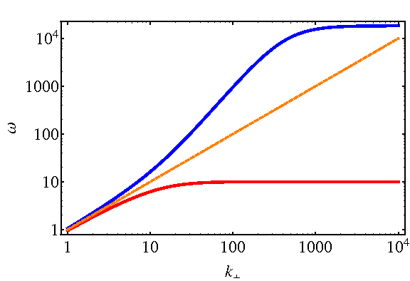
Figure 1: The dispersion relation $\left(w\right)$ profiles for $\theta=0$, $d_{i}=0.1$ and $d_{e}=0.0233$. The upper branch corresponds to whistler waves, while the lower branch represents ion cyclotron waves. The dashed reference line corresponding to ideal Alfvén waves which in dimensionless units is $w=k_{\bot}$.

V.1.2 Collisionless tearing modes

The XMHD model of (25)–(28) can describe various instabilities, including collisionless tearing modes induced by the presence of electron inertia, which breaks the usual MHD frozen-in condition as evidenced by Eqs. (25) and (27).

In order to investigate collisionless tearing, we suppose a resonant surface is located at $x=0$ and we choose an equilibrium around $x=0$ given by

$$\psi_{eq}=-x^{2},\qquad b_{eq}=0,\qquad\phi_{eq}=0,\qquad v_{eq}=0.$$ (97)

Then upon linearizing the system of (25)–(28) about this equilibrium, assuming solutions of the form $\psi(x,y,t)=\tilde{\psi}(x)\mathrm{e}^{iky+\gamma t}$ with analogous expressions for $\phi,v,$ and $b$, where the constants $\gamma$ and $k$ indicate the growth rate and the wave number of the perturbation, respectively, we obtain

$$g((1+k^{2}d_{e}^{2})\tilde{\psi}-d_{e}^{2}\tilde{\psi}^{\prime\prime}) = -ix(\tilde{\phi}+d_{i}\tilde{b}),$$ (98)

$$g(\tilde{\phi}^{\prime\prime}-k^{2}\tilde{\phi}) = -ix(\tilde{\psi}^{\prime\prime}-k^{2}\tilde{\psi}),$$ (99)

$$g((1+k^{2}d_{e}^{2})\tilde{b}-d_{e}^{2}\tilde{b}^{\prime\prime}) = ixd_{i}(\tilde{\psi}^{\prime\prime}-k^{2}\tilde{\psi})+ix\tilde{v},$$ (100)

$$g\tilde{v} = ix\tilde{b},$$ (101)

where $g=\gamma/(2k)$ and the prime symbol denotes derivative with respect to the argument. We remark then that the linear system (98)–(100) corresponds also to the linearization of the four-field model studied in Ref. Fit04, , provided one uses $\psi_{eq}=-x^{2}$ instead of $\psi_{eq}=-x^{2}/2$ and replaces the constant $d_{\beta}$ of Ref. Fit04, with the constant $d_{i}$ (which corresponds to taking the limit $\beta\rightarrow+\infty$). The additional terms of the model of (25)–(28) that are absent in the four-field model of Ref. Fit04, , indeed, contribute only during the nonlinear regime. We can then export the analysis carried out in Ref. Fit04, , where a relation for the growth rate in terms of equilibrium parameters was found by asymptotic matching. In this way we obtain the following expression for the growth rate for our system of (98)–(100):

$$-\frac{\pi}{\Delta^{\prime}}-\frac{\pi}{2}\frac{g^{2}}{d_{i}G(g/d_{i})}+\frac{d_{e}d_{i}G(g/d_{i})}{g}=0,$$ (102)

where $\Delta^{\prime}$ is the classical tearing stability parameter Fur63 and $G(x)=(\sqrt{x}/2)\Gamma(1/4+x/4)/\Gamma(3/4+x/4)$, with $\Gamma$ indicating the Gamma function. A version of the relation (102), adopting resistivity instead of electron inertia, has also been used in Ref. Baa11, for linear studies of reconnection based on 2D incompressible Hall MHD. The relation (102) is valid if the conditions $d_{e}\ll g\ll d_{i}\ll 1$ are satisfied.Fit04

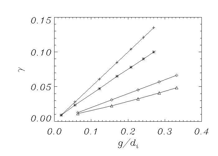
Figure 2: Comparison between values of the growth rate $\gamma$ obtained from numerical simulations and from the asymptotic relation (102), for different values of the parameter $g/d_{i}$. Crosses and asterisks indicate analytical and numerical values, respectively, for $d_{i}=0.5$, whereas diamonds and triangles correspond to analytical and numerical values, respectively, for $d_{i}=0.2$. For all cases $\Delta^{\prime}=59.9$.

In Fig. 2, values of the growth rate $\gamma$, obtained from the asymptotic relation (102), are checked against values obtained from numerical simulations, for a case with large $\Delta^{\prime}$. The numerical code used for these simulations is an adaptation of the one used in Ref. Grasso07, to solve the four-field system initialized by perturbing about the equilibrium

$$\psi_{eq}=\frac{1}{\cosh^{2}x},\qquad b_{eq}=\phi_{eq}=v_{eq}=0.$$ (103)

Note that the equilibrium (103), when expanded about $x=0$, corresponds to the equilibrium (97) adopted for deriving the analytical expression for the growth rate.

The model equations are solved on a grid consisting of up to 2048$\times$4096 grid points, depending on the scale lengths to be resolved. All the fields are split into the time-independent equilibrium and an evolving perturbation advanced in time by a third order Adams-Bashforth algorithm. Periodic boundary conditions have been imposed along the shear equilibrium magnetic field direction, $y$, whereas Dirichlet conditions have been applied in the $x$-direction with all the perturbed fields vanishing at the boundaries. A pseudospectral method is adopted for the periodic direction, while a compact finite difference algorithm on a non-equispaced grid is used for the spatial operations along the $x$ direction. The tearing instability is initiated by perturbing the equilibrium with a small disturbance of the parallel current density $j=-\nabla^{2}\psi$ of the form $\delta j\left({x,y}\right)=\delta j\left(x\right)\cos({{2\pi y}/{L_{y}}})$, where $\delta j\left(x\right)$ is a function localized within a width of order $d_{e}$ around the rational surface $x=0$.

One can observe from the figure that the agreement between numerical and analytical values becomes better and better as the parameter $g/d_{i}$ decreases. This is expected, since, the relation (102) holds in the asymptotic limit $g/d_{i}\ll 1$. We remark that, in the large $\Delta^{\prime}$ regime, in the limit $g/d_{i}\ll 1$, the relation (102) can be approximated by Fit04

$$g=\frac{1}{\sqrt{2\pi}}\frac{\Gamma(1/4)}{\Gamma(3/4)}\sqrt{d_{e}d_{i}},$$ (104)

which also shows the accelerating role played by the Hall term, associated with the length scale $d_{i}$.

V.2 Nonlinear numerical simulations

Having obtained a handle on the linear dynamics, we now describe our nonlinear numerical simulations. In particular, we follow the nonlinear evolution of the velocity and magnetic fields during the process of magnetic reconnection initiated by perturbing the equilibrium (103). The code employed is that of Sec. V.1.2.

Figure 3 shows contour plots of the out-of-plane magnetic and vorticity fields, at times well into the nonlinear regime, for two choices of skin depths with the same mass ratios. The two times, $126\tau_{A}$ for the case with $d_{e}=0.05,d_{i}=0.5$ and $56\tau_{A}$ for the case with $d_{e}=0.1,d_{i}=1$, were chosen because they represent approximately the same nonlinear stage. In both cases the field $b$ exhibits the characteristic quadrupolar structure, a signature of Hall reconnection (see, e.g., Refs. Yam10, ; Uzd06, ). In the case with the smaller skin depths, Figs. 3 and 3, one observes that the vorticity concentrates on a narrow region with a size of order of $d_{e}$. In this region the behavior is mainly dictated by incompressible hydrodynamics and the system can eventually become prone to the Kelvin-Helmholtz instability.Bis97 On the other hand, when increasing $d_{e}$ and $d_{i}$, as in Figs. 3 and 3, vorticity is no longer concentrated on a narrow region but distributes mainly along the island separatrices and inside the island over a region of width on the order of $d_{i}$, thus suppressing the Kelvin-Helmholtz instability. A similar mechanism for inhibiting a secondary Kelvin-Helmholtz instability was observed also for collisionless reconnection in the presence of a guide field in Refs. Del06, ; Gra09, ; Tas10, . In this case, the role of the Hall term was played by the electron pressure contribution to Ohm’s law. For completeness, we plot the remaining two fields at $126\tau_{A}$ in Fig. 4 with $v$ shown in Fig. 4 and $\psi$ in Fig. 4.

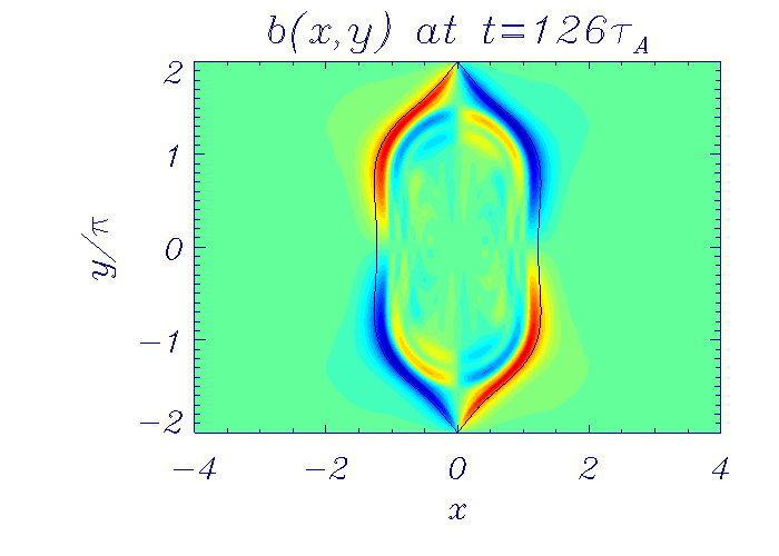
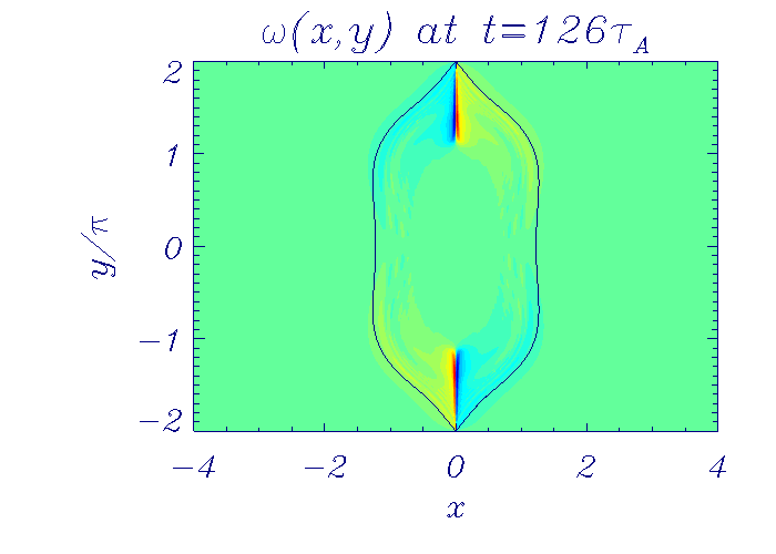
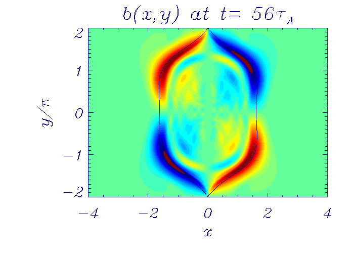
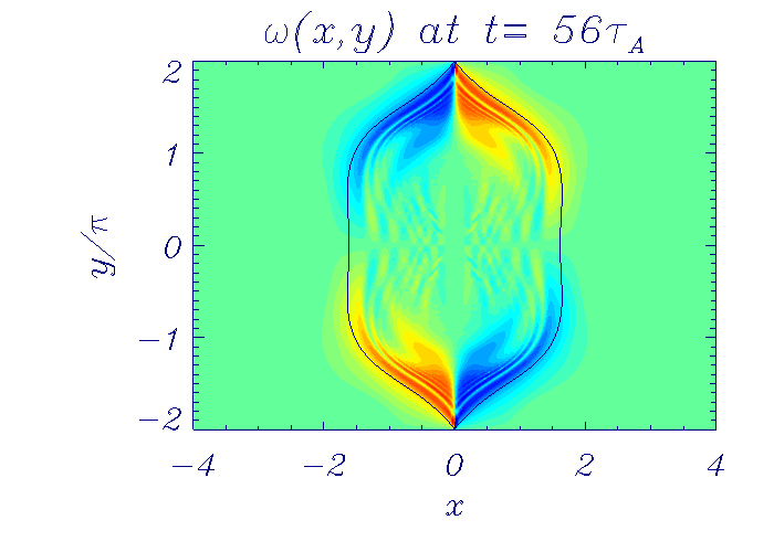
Figure 3: Contour plots of the out-of-plane magnetic field $b$ and vorticity $\omega$ at time $126\tau_{A}$ for $d_{e}=0.05$ and $d_{i}=0.5$ (Figs. 3 and 3) and at time $56\tau_{A}$ for $d_{e}=0.1$ and $d_{i}=1$ (Figs. 3 and 3) . The magnetic island is superimposed on the contour plots.

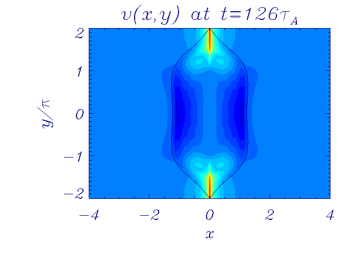
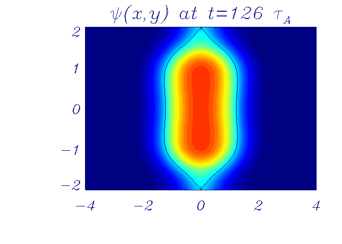
Figure 4: Contour plots of the velocity field $v$ Fig. 4 and flux $\psi$ Fig. 4 at time $126\tau_{A}$ for $d_{e}=0.05$ and $d_{i}=0.5$. The magnetic island is superimposed on the contour plots.

It is of interest to compare the four fields $(\omega,b,v,\psi)$ with the normal fields $(b_{\pm},\psi_{\pm})$ This is done in Fig. 5 for the smaller skin depths. As noted above in Figs. 3 and 3, $b$ and $\omega$ display the characteristic quadrupolar and current layer behavior, respectively, while from Figs. 4 and 4 the field $v$ is seen to display a sort of amorphous structure with a mixture of both features, while $\psi$ shows an elongated form with minimal current layer evidence. In comparison the normal fields of Fig. 5 reveal a cleaner separation of behavior, with $(b_{+},\psi_{+})$ displaying the current layer, which is notably absent in the normal fields $(b_{-},\psi_{-})$. Observe the amorphous behavior of $v$ is absent and the quadrupolar behavior of $b$ has now been concentrated along the magnetic island contour. We draw the conclusion that the normal fields more clearly delineate the nature of the evolution.

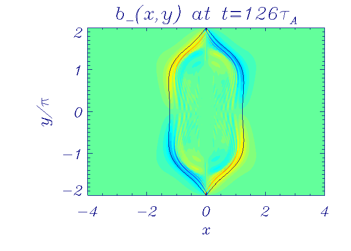
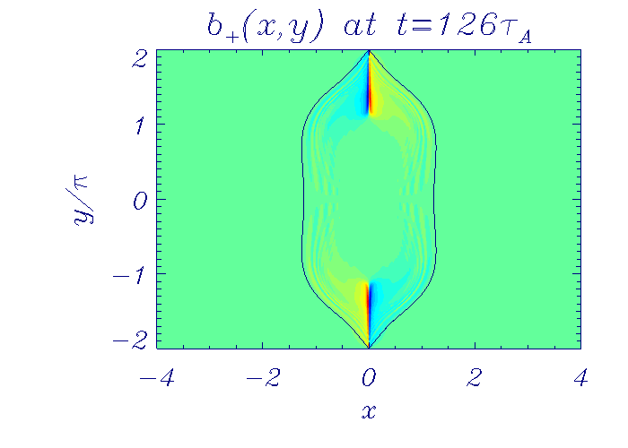
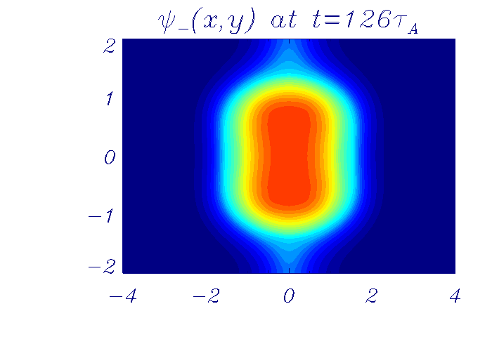
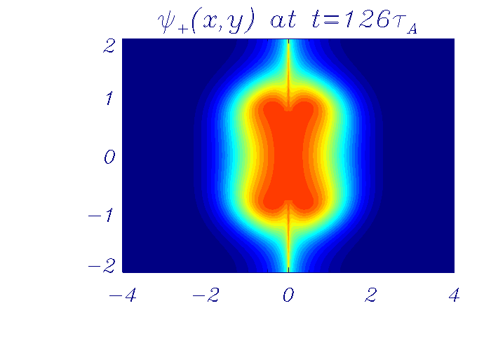
Figure 5: Contour plots of normal fields $(b_{\pm},\psi_{\pm})$ at time $126\tau_{A}$ for $d_{e}=0.05$ and $d_{i}=0.5$. The magnetic island is superimposed on the contour plots.

As noted in Sec. III.1, it is evident from Eqs. (52) that the normal fields $\psi_{\pm}$ correspond to the $z$-components of the electron and ion canonical momenta. It is important to recall that the notion of canonical momentum originates in the Hamiltonian formalism and, consequently, that they should play a clarifying role in the present application is not surprising. Because the fields $\psi_{\pm}$ are advected by the velocities associated with $\phi_{\pm}$ (cf.  Eqs. (50)), we examine the moduli $|\nabla\phi_{+}|$ and $|\nabla\phi_{-}|$ of the perpendicular velocities $\mathbf{V}_{\pm}=\widehat{z}\times\nabla\phi_{\pm}$ that are doing the advecting. Figure 6 shows profiles of the moduli at $y=0$, i.e. across the X-point. One observes that, in a narrow region around the resonant surface at $x=0$, the velocity $\mathbf{V}_{-}$, which is predominantly due to the electrons, dominates over the the velocity $\mathbf{V}_{+}$, which is predominantly due the ions and actually vanishes at $x=0$. This is consistent with the behavior described in Ref. Bis97, where magnetic flux bundle coalescence in a high $\beta$ regime was investigated. As discussed in Ref. Bis97, , this behavior can be explained considering that, in a region with the size $L\sim d_{e}\ll d_{i}$ around the resonant surface, the system (25)–(28) reduces to 2D electron MHD. The dynamics is then essentially governed by electron motion, whereas ions are immobile. On the other hand, on scales $L\geq d_{i}$, one enters an MHD regime, where $v_{e\perp}\approx v_{i\perp}$, as Fig. 6 shows with corrections due to the use of the normal fields.

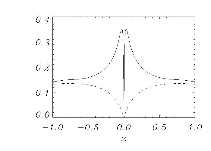
Figure 6: Plots of $|\nabla\phi_{+}|$ (dashed line) and $|\nabla\phi_{-}|$ (solid line) at $y=0$ and $t=126$.

The global structures of the velocities $\mathbf{V}_{\pm}$ are revealed in the contour plots of $\phi_{+}$ and $\phi_{-}$, respectively, shown in Fig. 7. As expected, upon comparing $\phi$ to $\phi_{+}$ it is seen that the bulk velocity is mostly due to the ion velocity, which exhibits the characteristic convective cells. The stream function $\phi_{-}$, associated with the corrected electron velocity, on the other hand, concentrates mainly in narrow structures along the separatrices. An analytical argument justifying such behavior of the electron velocity was provided in Ref. Bis97, , based on the electron MHD approximation, valid on scales much smaller than $d_{i}$.

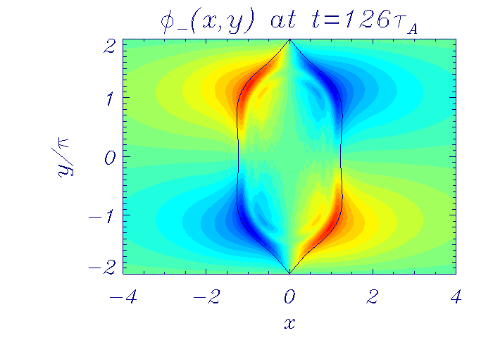
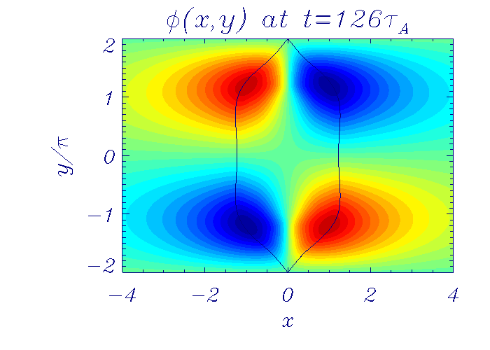
Figure 7: Contour plots of $\phi$ (left), $\phi_{+}$ (middle) and $\phi_{-}$ (right) for $d_{e}=0.05$ and $d_{i}=0.5$. The magnetic island is superimposed to the contour plots..

Because of the Hamiltonian nature of the model the total energy of (29) is conserved, yet during the course of the dynamics energy may transfer from one term to another. In order to track this we write

$$\mathscr{H}=\mathscr{H}_{\rm Kp}+\mathscr{H}_{\rm v}+\mathscr{H}_{\rm B}+\mathscr{H}_{\rm b}+\mathscr{H}_{\rm Ke}+\mathscr{H}_{\rm Kez}$$ (105)

with

$$\mathscr{H}_{\rm Kp} = \int\!d^{2}x\,|\nabla\phi|^{2}/2$$ (106)

$$\mathscr{H}_{\rm v} = \int\!d^{2}x\,v^{2}/2$$ (107)

$$\mathscr{H}_{\rm B} = \int\!d^{2}x\,|\nabla\psi|^{2}/2$$ (108)

$$\mathscr{H}_{\rm b} = \int\!d^{2}x\,b^{2}/2$$ (109)

$$\mathscr{H}_{\rm Ke} = \int\!d^{2}x\,d_{e}^{2}\,|\nabla^{2}\psi|^{2}/2$$ (110)

$$\mathscr{H}_{\rm Kez} = \int\!d^{2}x\,d_{e}^{2}\,|\nabla b|^{2}/2$$ (111)

and track each term during the reconnection process. Here, for convenience and physical clarity, we do this in terms of the original fields that appear in the Hamiltonian as a sum of squares, rather than evaluate the expression of (59) in terms of the normal fields. In Fig. 8 the total energy $\mathscr{H}$ is displayed as a solid line, showing that indeed the numerics preserves it well up to time $126\tau_{A}$ for our example with $d_{e}=0.05$ and $d_{i}=0.5$. Instead of plotting $\mathscr{H}$, we plot $E_{\rm tot}$, which is the total energy relative to the initial value of $\mathscr{H}$. The other energies of (106)-(111) are plotted similarly, e.g. $E_{\rm Kp}$ is the value of $\mathscr{H}_{\rm Kp}$, relative to $\mathscr{H}$. Next we observe that the energy $E_{\rm B}$ decreases while getting transferred to all of the other terms in varying amounts. The energy $E_{Ke}$, which is essentially the electron kinetic energy, gains only a small amount, as does the energy $E_{\rm Kez}$, which also contains higher order derivatives. Note both these energies are referred to the left hand scale. All of the other energies grow significantly more, but by far most of the energy goes into $E_{\rm Kp}$, the perpendicular kinetic energy, which significantly dominates $E_{\rm b}$, the parallel magnetic, and $E_{\rm v}$ parallel kinetic energies.

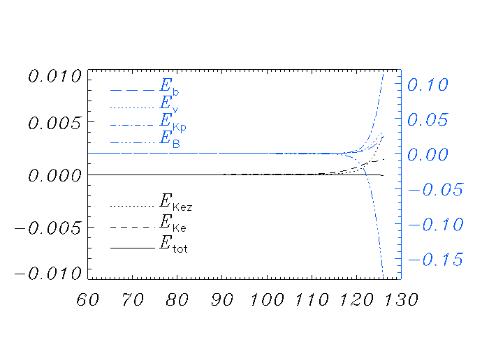
Figure 8: Temporal plots of the terms of the Hamiltonian ${\mathscr{H}}$ of (105) relative to their values at $t=0$ for parameters values $d_{e}=0.05$ and $d_{i}=0.5$. The total energy, represented by $E_{\rm tot}$, retains its initial value (solid line) throughout the simulation. The other terms, defined by (106)-(111), are seen to increase at the expense of the decreasing perpendicular magnetic energy $E_{\rm B}$ (dash-dot-dot-dot) with most energy going into the perpendicular kinetic energy $E_{\rm Kp}$ (dash-dot). Note that times before $t=60\tau_{A}$ are not shown because the dynamics is still in the linear phase where variations of all terms are negligible.

To compare these results with more conventional analyses we consider the approximate Hamiltonian of (60), which although not exactly conserved can be used to proved a physically transparent interpretation of the energy redistribution process during the reconnection. We write the approximate Hamiltonian $\tilde{\mathscr{H}}$ as the sum

$$\tilde{\mathscr{H}}=\tilde{\mathscr{H}}_{\rm B}+\tilde{\mathscr{H}}_{\rm i}+\tilde{\mathscr{H}}_{\rm e},$$ (112)

where $\tilde{\mathscr{H}}_{\rm B}=(1/2)\int d^{2}x(|\nabla\psi|^{2}+b^{2})$ is the total magnetic energy, $\tilde{\mathscr{H}}_{\rm i}=(1/2)\int d^{2}x(v_{i\perp}^{2}+v_{iz}^{2})$ is the total ion kinetic energy and $\tilde{\mathscr{H}}_{\rm e}=(1/2)(d_{e}^{2}/d_{i}^{2})\int d^{2}x\left(v_{e\perp}^{2}+v_{ez}^{2}\right)$ is the total electron kinetic energy. It is easy to infer from Fig. 8 that reconnection converts most of the magnetic energy into kinetic energy of the ion flow. This is consistent with what is heuristically mentioned in Ref. Bis97, , although the actual conserved energy was not identified in that reference.

VI Summary and Conclusions

In this paper we have given a comprehensive analysis of reduced extended MHD, a 2D version of extended MHD. We have derived the model starting from the Hamiltonian form of Lüst’s equations by a reduction procedure that produced the Hamiltonian form of the reduced model, RXMHD. This procedure led to the physical energy, which serves as the reduced Hamiltonian, the four families of Casimir invariants, and the definitions of the normal fields $(b_{\pm},\psi_{\pm})$ in terms of which the four equations of motion take a simplified intuitive form. Further reductions of the RXMHD led in a natural way to reduced Hall MHD, inertial MHD, and ideal MHD, Hamiltonian field theories with conserved energies and associated Casimir invariants. Analyses of RXMHD revealed the natural modes of oscillation, the expected whistler and ion cyclotron waves. The analytical expression for the linear collisionless tearing growth rate was inferred and checked against numerical solutions. Nonlinear simulations of collisionless tearing revealed behavior typical of Hall and electron inertia physics, but better organized by the new normal field variables.

The content of this work opens many avenues for further study, both analytical and numerical. We mention a few. On the analytical side one can effect absolute equilibrium calculations akin to those of Refs. HLS16, ; MLM16, in order to infer energy cascades. In addition one can derive the Hamiltonian form of 3D incompressible XMHD using the Dirac constraint technique of Ref. Cha12, and derive the weakly 3D version of the present model, where the latter gives rise to terms linear in parallel derivatives caused by a strong guide field. The general Hamiltonian form of such weakly 3D models is available in Ref. Tas10, and the correct one can be obtained by aspect ratio expansion of the full XMHD model or by Hamiltonian reduction. Having in hand the weakly 3D version of RXMHD opens the way for numerical treatment of weakly 3D collisionless tearing.

References

- (1) H. R. Strauss, Phys. Fluids 19, 134 (1976).
- (2) R. D. Hazeltine, M. Kotschenreuther, and P. J. Morrison, Phys. Fluids 28, 2466 (1985).
- (3) J. F. Drake and T. M. Antonsen, Jr., Phys. Fluids 27, 898 (1984).
- (4) A. Hasegawa and M. Wakatani, Phys. Fluids 26, 1770 (1983).
- (5) A. Brizard, Phys. Fluids B 4, 1213 (1992).
- (6) W. Dorland, G.W. Hammett, Phys. Fluids B 5, 812 (1993).
- (7) P.B. Snyder, G.W. Hammett, Phys. Plasmas 8, 3199 (2001).
- (8) D. Strintzi, B. D. Scott, and A. J. Brizard, Phys. Plasmas 12, 052517 (2005).
- (9) T. J. Schep, F. Pegoraro, and B. N. Kuvshinov, Phys. Plasmas
- (10) D. Grasso, F. Califano, F. Pegoraro, and F. Porcelli, Phys. Rev. Lett. 86, 5051 (2001).
- (11) D. Grasso, D. Borgogno and F. Pegoraro, Phys. Plasmas 14, 055703 (2007).
- (12) E. Tassi, P. J. Morrison, F. L. Waelbroeck, D. Grasso, Plasma Phys. and Control. Fusion 50, 085014 (2008).
- (13) F. L. Waelbroeck, R. D. Hazeltine, and P. J. Morrison Phys. Plasmas 16, 032109 (2009).
- (14) B. Scott, Phys. Plasmas 17, 102306 (2010).
- (15) F.L. Waelbroeck and E. Tassi, Commun. Nonlinear Sci. Numer. Simulat. 17, 2171 (2012).
- (16) I. Keramidas Charidakos, F. Waelbroeck, and P. J. Morrison, Physics of Plasmas 22, 112113 (2015).
- (17) P. J. Morrison and J. M. Greene, Phys. Rev. Lett. 45, 790 (1980).
- (18) P.J. Morrison, Rev. Mod. Phys. 70, 467 (1998).
- (19) P. J. Morrison, Phys.Plasmas 12, 058102 (2005).
- (20) P. J. Morrison and R.D. Hazeltine 27, 886 (1984).
- (21) J. E. Marsden and P. J. Morrison, Contemp. Math. 28 133 (1984)
- (22) C. T. Hsu, R. D. Hazeltine, and P. J. Morrison, Phys. Fluids 29, 1480 (1986).
- (23) R. D. Hazeltine, C. T. Hsu and P. J. Morrison, Phys. Fluids 30, 3204 (1987).
- (24) R. Lüst, Fortschritte der Physik 7, 503 (1959).
- (25) H. M. Abdelhamid, Y. Kawazura and Z. Yoshida, J. Phys. A 48, 235502 (2015).
- (26) M. Lingam, P. J. Morrison, and G. Miloshevich, Phys. Plasmas 22, 072111 (2015).
- (27) D. Biskamp, E. Schwarz, J. F. Drake, Phys. Plasmas 4, 1002 (1997).
- (28) D. Del Sarto, F. Califano, F. Pegoraro, Mod. Phys. Lett. B 20, 931 (2006).
- (29) D. Grasso, D. Borgogno, F. Pegoraro, E. Tassi, Nonlin. Processes Geophys. 16, 241 (2009).
- (30) E. Tassi, P. J. Morrison, D. Grasso, F. Pegoraro, Nucl. Fusion 50, 034007 (2010).
- (31) L. Comisso, D. Grasso, E. Tassi and F.L. Waelbroeck, Phys. Plasmas, 19, 042103 (2012).
- (32) N. Andres, L. Martin, P. Dmitruk and D. P. Gomez, Phys. Plasmas, 21, 072904 (2014).
- (33) K. Kimura and P. J. Morrison, Phys. Plasma 21, 082101 (2014).
- (34) T. Andreussi, P. J. Morrison, and F. Pegoraro, Plasma Phys. and Control. Fusion 52, 055001 (2010).
- (35) T. Andreussi, P. J. Morrison, and F. Pegoraro, Phys. Plasmas 19, 052102 (2012).
- (36) J. L. Thiffeault and P. J. Morrison, Physica D 136, 205 (2000).
- (37) H. M. Abdelhamid and Z. Yoshida, Phys. Plasmas 23, 022105 (2016).
- (38) R. Fitzpatrick and F. Porcelli, Phys. Plasmas 11, 4713 (2004).
- (39) H. P. Furth, J. Killeen and M. N. Rosenbluth, Phys. Fluids 6, 459 (1963).
- (40) S. D. Baalrud, A. Bhattacharjee, Y.-M. Huang and K. Germaschewski, Phys. Plasmas 18, 092108 (2011).
- (41) M. Yamada, R. Kulsrud, H. Ji, Rev. Mod. Phys. 82, 603 (2010).
- (42) D. A. Uzdensky, R. M. Kulsrud, Phys. Plasmas 13, 062305 (2006).
- (43) H. M. Abdelhamid, M. Lingam and S. M. Mahajan, Astrophys. J. 829, 87 (2016).
- (44) G. Miloshevich, M. Lingam, and P. J. Morrison. On the structure and statistical theory of turbulence of extended magnetohydrodynamics, arXiv:1610.04952v1 [physics.plasm-ph] (2016).
- (45) C. Chandre, P. J. Morrison and E. Tassi, Phys. Lett. A 376, 737 (2012).