Abstract

Recently, the regularized functional matching pursuit (RFMP) was introduced as a greedy algorithm for linear ill-posed inverse problems. This algorithm incorporates the Tikhonov-Phillips regularization which implies the necessity of a parameter choice. In this paper, some known parameter choice methods are evaluated with respect to their performance in the RFMP and its enhancement, the regularized orthogonal functional matching pursuit (ROFMP). As an example of a linear inverse problem, the downward continuation of gravitational field data from the satellite orbit to the Earth’s surface is chosen, because it is exponentially ill-posed. For the test scenarios, different satellite heights with several noise-to-signal ratios and kinds of noise are combined. The performances of the parameter choice strategies in these scenarios are analyzed. For example, it is shown that a strongly scattered set of data points is an essentially harder challenge for the regularization than a regular grid. The obtained results yield a first orientation which parameter choice methods are feasible for the RFMP and the ROFMP.

Key words: gravitational field, ill-posed, inverse problem, parameter choice methods, regularization, sphere

MSC2010: 65N21, 65R32, 86A22

1 Introduction

The gravitational field of the Earth is an important reference in the geosciences. It is an indicator for mass transports and mass reallocation on the Earth’s surface. These displacements of masses can be caused by ocean currents, evaporation, changes of the groundwater level, ablating of continental ice sheets, changes in the mean sea level or climate change (see e.g. [18, 19]).
However, it is difficult to model the gravitational field, because terrestrial measurements are not globally available. In addition, the points of measurement on the sea are more scattered than those on the continents. This has motivated the launch of satellite missions with a focus on the gravitational field (see e.g. [8, 31, 37, 41]). Naturally, those data are given at a satellite orbit, not on the Earth’s surface. Additionally, the measurements are only given pointwise and are afflicted with noise. The problem of getting the potential from the satellite orbit onto the Earth’s surface is the so-called downward continuation problem, which is a severely unstable and, therefore, ill-posed inverse problem (see e.g. [13, 40]).
Traditionally, the gravitational potential of the Earth has been represented in terms of orthogonal spherical polynomials (i.e. spherical harmonics $Y_{n,j}$, see e.g. [12, 23, 30]) as in the case of the Earth Gravitational Model 2008 (EGM2008, see [33]). An advantage of this representation is that the upward continuation operator $\Psi$ which maps a potential $F$ from the Earth’s surface (which we assume here to be the unit sphere $\Omega$) to the orbit $r\Omega$ with $r>1$ has the singular value decomposition

$$\left(\Psi F\right)\left(x\right)=\sum\limits_{n=0}^{\infty}\sum\limits_{j=-n}^{n}\left\langle F,Y_{n,j}\right\rangle_{\mathrm{L}^{2}(\Omega)}r^{-n}\,Y_{n,j}^{r}\left(x\right),$$ (1)

where $Y_{n,j}^{r}(x)\coloneqq\frac{1}{r}Y_{n,j}\left(\frac{x}{r}\right)$, $x\in r\Omega$. Its inverse is, therefore, given by

$$\Psi^{+}G=\sum\limits_{n=0}^{\infty}\sum\limits_{j=-n}^{n}\left\langle G,Y_{n,j}^{r}\right\rangle_{\mathrm{L}^{2}(r\Omega)}r^{n}Y_{n,j}=\sum\limits_{n=0}^{\infty}\sum\limits_{j=-n}^{n}\left\langle G,Y_{n,j}^{r}\right\rangle_{\mathrm{L}^{2}(r\Omega)}\sigma_{n}^{-1}Y_{n,j}$$ (2)

in the sense of $\mathrm{L}^{2}(\Omega)$ and for all $G\in\Psi(\mathrm{L}^{2}(\Omega))\subset\mathrm{L}^{2}(r\Omega)$. Note that the singular values of $\Psi^{+}$, which are given by $(\sigma_{n}^{-1})_{n}=(r^{n})_{n}$, increase exponentially. For details, see [40, 42].

The outline of this paper is as follows. Section 2 deals with the RFMP and its enhancement, the ROFMP, which are used here for the regularization of $\Psi^{+}$. For both algorithms, the essential theoretical results are recapitulated. In Section 3, the parameter choice methods under consideration for the RFMP and ROFMP are summarized and details of their implementation for the test cases are explained. In Section 4, the relevant details of the considered test scenarios are outlined. Section 5 analyzes and compares the results for the various parameter choice strategies.

2 RFMP

In this section, we briefly resume the regularized functional matching pursuit (RFMP), which was introduced in [9, 10, 24, 26], and an orthogonalized modification of it (see [27, 42]). It is an algorithm for the regularization of linear inverse problems.

According to [25, 26, 42], we use an arbitrary Hilbert space $\mathcal{H}\subset\mathrm{L}^{2}(\Omega)$.
Let an operator $\mathcal{F}:\mathcal{H}\rightarrow\mathbb{R}^{l}$ be given which is continuous and linear. Concerning the downward continuation, we have a vector $\boldsymbol{y}\in\mathbb{R}^{l}$ of measurements at a satellite orbit, that means our data are given pointwise. The inverse problem consists of the determination of a function $F\in\mathcal{H}$ such that

$$\mathcal{F}F=\boldsymbol{y}=((\Psi F)(x_{j}))_{j=1,\dots,l},$$ (3)

where $(x_{j})_{j=1,\dots,l}$ is a set of points at satellite height. In the following, we use bold letters for vectors in $\mathbb{R}^{l}$.

To find an approximation for our function F, we need to have a set of trial functions $\mathcal{D}\subset\mathcal{H}\setminus\{0\}$, which we call the dictionary. Our unknown function $F$ is expanded in terms of dictionary elements, that means we can represent it as $F=\sum_{k=1}^{\infty}\alpha_{k}d_{k}\mathrm{\leavevmode\nobreak\ with\leavevmode\nobreak\ }\alpha_{k}\in\mathbb{R}\mathrm{\leavevmode\nobreak\ and\leavevmode\nobreak\ }d_{k}\in\mathcal{D}\mathrm{\leavevmode\nobreak\ for\leavevmode\nobreak\ all\leavevmode\nobreak\ }k\in\mathbb{N}$.

2.1 The algorithm

The idea of the RFMP is the iterative construction of a sequence of approximations $(F_{n})_{n}$. This means that we add a basis function $d_{k}$ of the dictionary to the approximation in each step. This basis function is furthermore equipped with a coefficient $\alpha_{k}$.

Since the considered inverse problem is ill-posed, we use the Tikhonov-Phillips regularization, that is, our task is to find a function $F$ which minimizes

$$\left\|\boldsymbol{y}-\mathcal{F}F\right\|_{\mathbb{R}^{l}}^{2}+\lambda\left\|F\right\|_{\mathcal{H}}^{2}.$$ (4)

That means, if we have the approximation $F_{n}$ up to step $n$, our greedy algorithm chooses $\alpha_{n+1}\in\mathbb{R}$ and $d_{n+1}\in\mathcal{D}$ such that

$$\left\|\boldsymbol{y}-\mathcal{F}\left(F_{n}+\alpha_{n+1}d_{n+1}\right)\right\|_{\mathbb{R}^{l}}^{2}+\lambda\left\|F_{n}+\alpha_{n+1}d_{n+1}\right\|_{\mathcal{H}}^{2}$$ (5)

is minimized. Here, $\lambda>0$ is the regularization parameter.

We can state the following algorithm for the RFMP.

Algorithm 2.1.

Let $\boldsymbol{y}\in\mathbb{R}^{l}$ and an operator $\mathcal{F}:\mathcal{H}\rightarrow\mathbb{R}^{l}$ (linear and continuous) be given.

(1) Initialization

Set $n\coloneqq 0$, $F_{0}\coloneqq 0$ and $\boldsymbol{R}_{0}\coloneqq\boldsymbol{y}-\mathcal{F}F_{0}=\boldsymbol{y}$, choose a stopping criterion (we stop, if $\left\|\boldsymbol{R}_{n+1}\right\|<\varrho$ for a given $\varrho>0$ or $\alpha_{n+1}<\delta$ for a given $\delta>0$ or $n+1>N$ for a given $N\in\mathbb{N}$, see also Section 4.1), and choose a regularization parameter $\lambda\in\mathbb{R}^{+}$.

(2) Iteration

Build $F_{n+1}\coloneqq F_{n}+\alpha_{n+1}d_{n+1}$ such that the following is fulfilled:

$$d_{n+1} \coloneqq\operatorname*{argmax}_{d\in\mathcal{D}}\frac{\left(\left\langle\boldsymbol{R}_{n},\mathcal{F}d\right\rangle_{\mathbb{R}^{l}}-\lambda\left\langle F_{n},d\right\rangle_{\mathcal{H}}\right)^{2}}{\left\|\mathcal{F}d\right\|_{\mathbb{R}^{l}}^{2}+\lambda\left\|d\right\|_{\mathcal{H}}^{2}},$$ (6)

$$\alpha_{n+1} \coloneqq\frac{\left\langle\boldsymbol{R}_{n},\mathcal{F}d_{n+1}\right\rangle_{\mathbb{R}^{l}}-\lambda\left\langle F_{n},d_{n+1}\right\rangle_{\mathcal{H}}}{\left\|\mathcal{F}d_{n+1}\right\|_{\mathbb{R}^{l}}^{2}+\lambda\left\|d_{n+1}\right\|_{\mathcal{H}}^{2}}.$$ (7)

Set $\boldsymbol{R}_{n+1}\coloneqq\boldsymbol{R}_{n}-\alpha_{n+1}\mathcal{F}d_{n+1}$.

(3) Stopping criterion

$F_{n+1}$ is the output, if the stopping criterion is fulfilled. Otherwise, increase $n$ and go to step 2.

The maximization, which is necessary to get $d_{n+1}$, is implemented by evaluating the fraction for all $d\in\mathcal{D}$ in each iteration and picking a maximizer. Since many involved terms can be calculated in a preprocessing, the numerical expenses can be kept low (see [24]). For a convergence proof of the RFMP, we refer to [25]. Briefly, under certain conditions, one can show that the sequence $(F_{n})_{n}$ converges to the solution $F_{\infty}$ of the Tikhonov-regularized normal equation

$$(\mathcal{F}^{*}\mathcal{F}+\lambda\mathcal{I})F_{\infty}=\mathcal{F}^{*}y,$$ (8)

where $\mathcal{I}$ is the identity operator and $\mathcal{F}^{*}$ is the adjoint operator to $\mathcal{F}$.

2.2 ROFMP

The regularized orthogonal functional matching pursuit (ROFMP) is an advancement of the RFMP from the previous section.

The basic idea is to project the residual onto the span of the chosen vectors, i.e.,

$$\mathcal{V}_{n}\coloneqq\operatorname{span}\{\mathcal{F}d_{1},\dots,\mathcal{F}d_{n}\}\subset\mathbb{R}^{l}\,,$$ (9)

and then adjust the previously chosen coefficients in such a way that the residual is afterwards contained in the orthogonal complement of the span. Since this so-called backfitting (cf. [22, 32]) might not be optimal, we implement the so-called prefitting (cf. [45]), where the next function and all coefficients are chosen simultaneously to guarantee optimality at every single stage of the algorithm. Moreover, let $\mathcal{W}_{n}\coloneqq\mathcal{V}_{n}^{\bot}$ and the orthogonal projections on $\mathcal{V}_{n}$ and $\mathcal{W}_{n}$ are denoted by $\mathcal{P}_{\mathcal{V}_{n}}$ and $\mathcal{P}_{\mathcal{W}_{n}}$, respectively. All in all, our aim is to find

$$\left(\alpha_{n+1},d_{n+1}\right)=\operatorname*{argmin}_{\alpha\in\mathbb{R},\,d\in\mathcal{D}}\left(\left\|\boldsymbol{R}_{n}-\alpha\mathcal{P}_{\mathcal{W}_{n}}\mathcal{F}d\right\|_{\mathbb{R}^{l}}^{2}+\lambda\left\|F_{n}-\alpha B_{n}(d)+\alpha d\right\|_{\mathcal{H}}^{2}\right).$$ (10)

Here,

$$\sum_{i=1}^{n}\beta_{i}^{(n)}(d)\mathcal{F}d_{i}=\mathcal{P}_{\mathcal{V}_{n}}(\mathcal{F}d)$$ (11)

and, thereby, we set

$$B_{n}(d)\coloneqq\sum_{i=1}^{n}\beta_{i}^{(n)}(d)d_{i}\in\mathcal{H}.$$ (12)

The updated coefficients for the expansion at step $n+1$ are given by

$$\alpha_{i}^{(n+1)}\coloneqq \alpha_{i}^{(n)}-\alpha_{n+1}\beta_{i}^{(n)}(d_{n+1}),\quad i=1,\dots,n,$$ (13)

$$\alpha_{n+1}^{(n+1)}\coloneqq \alpha_{n+1}.$$ (14)

The ROFMP algorithm can be summarized as follows.

Algorithm 2.2.

Let a dictionary $\mathcal{D}\subset\mathcal{H}$, a data vector $\boldsymbol{y}\in\mathbb{R}^{l}$ and an operator $\mathcal{F}:\mathcal{H}\rightarrow\mathbb{R}^{l}$ (linear and continuous) be given.

(1) Initialization

Set $n\coloneqq 0$, $F_{0}\coloneqq 0$ and $\boldsymbol{R}_{0}\coloneqq\boldsymbol{y}$, choose a stopping criterion (we stop, if $\left\|\boldsymbol{R}_{n+1}\right\|<\varrho$ for a given $\varrho>0$ or $\alpha_{n+1}<\delta$ for a given $\delta>0$ or $n+1>N$ for a given $N\in\mathbb{N}$, see also Section 4.1), and choose a regularization parameter $\lambda\in\mathbb{R}^{+}$.

(2) Iteration

Choose a function

$$d_{n+1}\coloneqq\operatorname*{argmax}\limits_{d\in\mathcal{D}}\frac{\left(\left\langle\boldsymbol{R}_{n},\mathcal{P}_{\mathcal{W}_{n}}\mathcal{F}d\right\rangle_{\mathbb{R}^{l}}+\lambda\left(\left\langle F_{n},B_{n}(d)\right\rangle_{\mathcal{H}}-\left\langle F_{n},d\right\rangle_{\mathcal{H}}\right)\right)^{2}}{\left\|\mathcal{P}_{\mathcal{W}_{n}}\mathcal{F}d\right\|_{\mathbb{R}^{l}}^{2}+\lambda\left(\left\|d-B_{n}(d)\right\|_{\mathcal{H}}^{2}\right)},$$ (15)

and calculate the corresponding coefficient

$$\alpha_{n+1}\coloneqq\frac{\left\langle\boldsymbol{R}_{n},\mathcal{P}_{\mathcal{W}_{n}}\mathcal{F}d_{n+1}\right\rangle_{\mathbb{R}^{l}}+\lambda\left(\left\langle F_{n},B_{n}(d_{n+1})\right\rangle_{\mathcal{H}}-\left\langle F_{n},d_{n+1}\right\rangle_{\mathcal{H}}\right)}{\left\|\mathcal{P}_{\mathcal{W}_{n}}\mathcal{F}d_{n+1}\right\|_{\mathbb{R}^{l}}^{2}+\lambda\left\|d_{n+1}-B_{n}(d_{n+1})\right\|_{\mathcal{H}}^{2}},$$ (16)

where $B_{n}(d)$ is defined according to (11) and (12). With the updated coefficients $\alpha_{i}^{(n+1)}\coloneqq\alpha_{i}^{(n)}-\alpha_{n+1}\beta_{i}^{(n)}(d_{n+1})$ for $i=1,\dots,n$, we set $\alpha_{n+1}^{(n+1)}\coloneqq\alpha_{n+1}$ and build $F_{n+1}\coloneqq\sum_{i=1}^{n+1}\alpha_{i}^{(n+1)}d_{i}$. Finally, update the residual $\boldsymbol{R}_{n+1}\coloneqq\boldsymbol{R}_{n}-\alpha_{n+1}\mathcal{P}_{\mathcal{W}_{n}}\mathcal{F}d_{n+1}$.

(3) Stopping criterion

$F_{n+1}$ is the output, if the stopping criterion is fulfilled. Otherwise, increase $n$ and go to step 2.

For practical details of the implementation, see [42].

Remark 2.3.

If we choose $d_{i}\in\mathcal{D}$ and $\alpha_{i}$ as in Algorithm 2.2 and update $\alpha$ as in (13) and (14), we obtain for the regularized case $(\lambda>0)$ that $\boldsymbol{R}_{n}$ is, in general, not orthogonal to $\mathcal{V}_{n}$ for all $n\in\mathbb{N}_{0}$, that means

$$\boldsymbol{R}_{n}\notin\mathcal{W}_{n}.$$ (17)

In [42], it was shown that, with the assumptions from Remark 2.3, there exists a number $N:=N(\lambda)$ such that

$$\boldsymbol{R}_{n}=\boldsymbol{R}_{N}\mathrm{\leavevmode\nobreak\ for\leavevmode\nobreak\ all\leavevmode\nobreak\ }n\geq N.$$ (18)

That means we get a stagnation of the residual. This is a problem for the ROFMP, because we cannot reconstruct a certain part of the signal which lies in $\mathcal{V}_{n}$. Therefore, we have to modify the algorithm to an iterated Tikhonov-Phillips regularization. That means we run the algorithm for a given number of iterations (in our case $K>0$), then break up the process and start the algorithm again with the previous residual $\boldsymbol{R}_{K}$. This is called the restart or repetition. For this process, we first need an additional notation: we add a further subscript $j$ to the expansion $F_{n}$. Note that we have two levels of iterations here. The upper level is associated to the restart procedure and is enumerated by the second subscript $j$. The lower iteration level is the previously described ROFMP iteration with the first subscript $n$. We denote the current expansion by

$$F_{n,j}\coloneqq F_{K,j-1}+\sum\limits_{i=1}^{n}\alpha_{i,j}^{(n)}d_{i,j},$$ (19)

where $F_{0,1}\coloneqq 0$ and $F_{0,j}\coloneqq F_{K,j-1}$. In analogy to the previous definitions, the residual can be defined in the following way:

$$\boldsymbol{R}_{n,j}\coloneqq\boldsymbol{y}-\mathcal{F}F_{n,j},\,1\leq n\leq K,\,j\geq 1\mathrm{\leavevmode\nobreak\ and\leavevmode\nobreak\ }\boldsymbol{R}_{0,j}\coloneqq\boldsymbol{y}-\mathcal{F}F_{K,j-1}=\boldsymbol{R}_{K,j-1}.$$ (20)

That means, after $K$ iterations, we keep the previously chosen coefficients fixed and restart the ROFMP with the residual of the step before. All in all, we have to solve

$$\left(\alpha_{n+1,j},d_{n+1,j}\right)=\operatorname*{argmin}_{\alpha\in\mathbb{R},\,d\in\mathcal{D}}\left(\left\|\boldsymbol{R}_{n,j}-\alpha\mathcal{P}_{\mathcal{W}_{n,j}}\mathcal{F}d\right\|_{\mathbb{R}^{l}}^{2}+\lambda\left\|F_{n+1,j}\right\|_{\mathcal{H}}^{2}\right)$$ (21)

and update the coefficients in the following way

$$\alpha_{i,j}^{(n+1)}:=\alpha_{i,j}^{(n)}-\alpha_{n+1,j}\beta_{i,j}^{(n)}(d_{n+1,j}),\quad i=1,\dots,n.$$ (22)

We summarize for the expansion $F_{K,m}$, which is the approximation produced by the ROFMP after $m$ restarts:

$$T_{m}:=F_{K,m}=\sum\limits_{j=1}^{m}\sum\limits_{i=1}^{K}\alpha_{i,j}^{(K)}d_{i,j}.$$ (23)

In analogy to the RFMP, we obtain a similar convergence result for the ROFMP. That is, under certain technical conditions, the sequence $(T_{m})_{m}$ converges in the Sobolev space $\mathcal{H}$. For further details, we refer to [27, 42].

3 Parameter choice methods

The choice of the regularization parameter $\lambda$ is crucial for the RFMP and the ROFMP, as for every other regularization method. In this section, we briefly summarize the parameter choice methods which we test for the RFMP and the ROFMP. This section is basically conform to [1, 2].

3.1 Introduction

The Earth Gravitational Model 2008 (EGM2008, see [33]) is a spherical harmonics model of the gravitational potential of the Earth up to degree $2190$ and order $2159$. We use this model up to degree $100$ for the solution $F$ in our numerical tests. For checking the parameter choice methods, we generate different test cases that means test scenarios which vary in the satellite height, the noise-to-signal ratio and the data grid. Based on the chosen function $F$, our dictionary contains all spherical harmonics up to degree $100$ that means our approximation $F$ from the algorithm has the following representation

$$F=\sum\limits_{n=0}^{100}\sum\limits_{j=-n}^{n}\alpha_{n,j}Y_{n,j},\mathrm{\leavevmode\nobreak\ where\leavevmode\nobreak\ not\leavevmode\nobreak\ all\leavevmode\nobreak\ }\alpha_{n,j}\mathrm{\leavevmode\nobreak\ vanish}.$$ (24)

This is a strong limitation, but higher degrees would essentially enlarge the computational expenses.

Moreover, for the stabilization of the solution, we use the norm of the Sobolev space $\mathcal{H}:=\mathcal{H}((a_{n})_{n};\Omega)$ which is constructed with

$$a_{n}\coloneqq\left(n+\frac{1}{2}\right)^{2},n\in\mathbb{N}_{0},$$ (25)

see [11]. This Sobolev space contains all functions $F$ on $\Omega$ which fulfil

$$\sum_{n=0}^{\infty}\sum_{j=-n}^{n}a_{n}^{2}\left\langle F,Y_{n,j}\right\rangle_{\mathrm{L}^{2}(\Omega)}^{2}<\infty.$$ (26)

The inner product of functions $F,G\in\mathcal{H}$ is given by

$$\left\langle F,G\right\rangle_{\mathcal{H}}\coloneqq\sum_{n=0}^{\infty}\sum_{j=-n}^{n}a_{n}^{2}\left\langle F,Y_{n,j}\right\rangle_{\mathrm{L}^{2}(\Omega)}\left\langle G,Y_{n,j}\right\rangle_{\mathrm{L}^{2}(\Omega)}.$$ (27)

The particular sequence $(a_{n})_{n}=((n+\frac{1}{2})^{2})$ was chosen, because preliminary numerical experiments showed that the associated regularization term yielded results with an appropriate smoothness.

In our test scenarios, we use a finite set $\{\lambda_{k}\}_{k=1,\dots,100}$ of $100$ regularization parameters (for details, see Section 4.4). The approximate solution of the inverse problem as an output of the RFMP/ROFMP corresponding to the regularization parameter $\lambda_{k}$ and the data vector $\boldsymbol{y}$ is denoted by $x_{k}$. This notation is introduced to avoid confusions with the functions $F_{n}$ which occur at the $n$-th step of the iteration within the RFMP.

In practice, we deal with noisy data $\boldsymbol{y}^{\varepsilon}$ where the noise level $\varepsilon$ is defined by

$$\varepsilon\coloneqq\mathrm{N2S}\cdot\left\|\boldsymbol{y}\right\|_{\mathbb{R}^{l}}/\sqrt{l},$$ (28)

where $l$ is the length of the data vector $\boldsymbol{y}$ and N2S is called the noise-to-signal ratio. The corresponding result of the RFMP/ROFMP for the regularization parameter $\lambda_{k}$ and the noisy data vector $\boldsymbol{y}^{\varepsilon}$ is called $x_{k}^{\varepsilon}$. Due to the convergence results for the RFMP/ROFMP (see (8)), we introduce the linear regularization operators $\mathcal{R}_{k}:\mathbb{R}^{l}\rightarrow\mathcal{H}$,

$$\mathcal{R}_{k}\coloneqq(\mathcal{F}^{*}\mathcal{F}+\lambda_{k}\mathcal{I})^{-1}\mathcal{F}^{*}$$ (29)

and assume $x_{k}$ to be $\mathcal{R}_{k}\boldsymbol{y}$ and $x_{k}^{\varepsilon}$ to be $\mathcal{R}_{k}\boldsymbol{y^{\varepsilon}}$, though this could certainly only be guaranteed for an infinite number of iterations.

Due to the importance of the regularization parameter, we summarize in the next section some methods for the choice of this parameter $\lambda$. For the comparison of the methods, we have to define the optimal regularization parameter $\lambda_{k_{\mathrm{opt}}}$. We do this by minimizing the difference between the exact solution $x$ and the regularized solution $x_{k}^{\varepsilon}$ corresponding to the parameter $\lambda_{k}$ and noisy data.

$$k_{\mathrm{opt}}\coloneqq\operatorname*{argmin}_{k\in\{1,\dots,100\}}\|x-x_{k}^{\varepsilon}\|_{\mathrm{L}^{2}(\Omega)}.$$ (30)

Then we evaluate the results by computing the so-called inefficiency by

$$\frac{\left\|x-x_{k_{*}}^{\varepsilon}\right\|_{\mathrm{L}^{2}(\Omega)}}{\left\|x-x_{k_{\mathrm{opt}}}^{\varepsilon}\right\|_{\mathrm{L}^{2}(\Omega)}},$$ (31)

where $\lambda_{k_{*}}$ is the regularization parameter selected by the considered parameter choice method. For the computation of the inefficiency, we use the $\mathrm{L}^{2}(\Omega)$-norm, since our numerical results led to a better distinction of the different inefficiencies than by using the $\mathcal{H}$-norm. However, the tendency regarding ’good’ and ’bad’ parameters were the same in both cases. The closer the obtained inefficiency is to 1, the better the parameter choice method performs.

The norms which occur in the several parameter choice methods can be computed with the help of the singular value decomposition. However, we use the singular values of $\Psi$ (see (1) and (3)) for this purpose, because the singular value decomposition of $\mathcal{F}$ is unavailable. This certainly causes an inaccuracy in our calculations, but appears to be unavoidable for the sake of practicability.

3.2 Parameter Choice Methods

Table 1 shows the different parameter choice methods we tested. The tuning parameters are chosen in accordance to [1, 2]. For the choice of the maximal index $\hat{K}$, see Section 4.5.

Name	Selection criterion	Specifications
Discrepancy Principle (DP)	Choose the first $k$ such that	Tuning parameter $\tau>1$.
(References: [28, 29, 34])	$\|\mathcal{F}x_{k}^{\varepsilon}-\boldsymbol{y}^{\varepsilon}\|_{\mathbb{R}^{l}}\leq\tau\varepsilon\sqrt{l}$.	(We choose $\tau=1.5$.)
Transformed Discrepancy Principle (TDP)	Choose the first $k$ such that	Tuning parameter $b>\gamma=((1/4)^{(1/4)}(3/4)^{(3/4)})^{2}$,
(References: [35, 36])	$\|\mathcal{R}_{k}(\mathcal{F}x_{k}^{\varepsilon}-\boldsymbol{y}^{\varepsilon})\|_{\mathcal{H}}\leq b\hat{\varepsilon}\frac{\sqrt{l}}{\sqrt{\lambda_{k}}}$.	estimate $\hat{\varepsilon}$ of $\varepsilon$. (We choose $b=1.5\gamma$ and $\hat{\varepsilon}=\varepsilon$.)
Quasi-optimality Criterion (QOC)	$k_{*}=\operatorname*{argmin}\limits_{k\leq\hat{K}}\|x_{k}^{\varepsilon}-x_{k+1}^{\varepsilon}\|_{\mathcal{H}}$
(References: [43, 44])
L-curve Method (LC)	$k_{*}=\operatorname*{argmin}\limits_{k\leq\hat{K}}\{\|\mathcal{F}x_{k}^{\varepsilon}-\boldsymbol{y}^{\varepsilon}\|_{\mathbb{R}^{l}}\cdot\|x_{k}^{\varepsilon}\|_{\mathcal{H}}\}$
(References: [14, 15, 16])
Extrapolated Error Method (EEM)	$k_{*}=\operatorname*{argmin}\limits_{k\leq\hat{K}}\Big{\{}\frac{\|\mathcal{F}x_{k}^{\varepsilon}-\boldsymbol{y}^{\varepsilon}\|_{\mathbb{R}^{l}}^{2}}{\|\mathcal{F}^{*}(\mathcal{F}x_{k}^{\varepsilon}-\boldsymbol{y}^{\varepsilon})\|_{\mathcal{H}}}\Big{\}}$
(References: [4, 5])
Residual Method (RM)	$k_{*}=\operatorname*{argmin}\limits_{k\leq\hat{K}}\Big{\{}\frac{\|\mathcal{F}x_{k}^{\varepsilon}-\boldsymbol{y}^{\varepsilon}\|_{\mathbb{R}^{l}}}{(\mathrm{tr}\mathcal{B}^{*}\mathcal{B})^{1/4}}\Big{\}}$,
(References: [3])	where $\mathcal{B}=\mathcal{F}(\mathcal{I}-\mathcal{R}_{k}\mathcal{F})$.
Generalized Maximum Likelihood (GML)	$k_{*}=\operatorname*{argmin}\limits_{k\leq\hat{K}}\Big{\{}\frac{\|\mathcal{F}x_{k}^{\varepsilon}-\boldsymbol{y}^{\varepsilon}\|_{\mathbb{R}^{l}}^{2}}{(\mathrm{det}^{+}(\mathcal{I}-\mathcal{F}\mathcal{R}_{k}))^{1/l_{1}}}\Big{\}}$	$l_{1}=\mathrm{rank}(\mathcal{I}-\mathcal{F}\mathcal{R}_{k})$. (In our case $l_{1}=l$.)
(References: [48])		$\mathrm{det}^{+}$ is the product of the nonzero eigenvalues.
Generalized Cross Validation (GCV)	$k_{*}=\operatorname*{argmin}\limits_{k\leq\hat{K}}\Big{\{}\frac{\left\|\mathcal{F}x_{k}^{\varepsilon}-\boldsymbol{y}^{\varepsilon}\right\|_{\mathbb{R}^{l}}^{2}}{(l^{-1}\mathrm{tr}(\mathcal{I}-\mathcal{F}\mathcal{R}_{k}))^{2}}\Big{\}}$
(References: [47])
Robust GCV (RGCV)	$k_{*}=\operatorname*{argmin}\limits_{k\leq\hat{K}}\Big{\{}\frac{\left\|\mathcal{F}x_{k}^{\varepsilon}-\boldsymbol{y}^{\varepsilon}\right\|_{\mathbb{R}^{l}}^{2}}{(l^{-1}\mathrm{tr}(\mathcal{I}-\mathcal{F}\mathcal{R}_{k}))^{2}}$	Robustness parameter $\gamma\in(0,1)$.
(References: [20, 39])	$\times\left(\gamma+(1-\gamma)l^{-1}\mathrm{tr}((\mathcal{F}\mathcal{R}_{k})^{2})\right)\Big{\}}$	(We choose $\gamma=0.1$.)
Strong RGCV (SRGCV)	$k_{*}=\operatorname*{argmin}\limits_{k\leq\hat{K}}\Big{\{}\frac{\left\|\mathcal{F}x_{k}^{\varepsilon}-\boldsymbol{y}^{\varepsilon}\right\|_{\mathbb{R}^{l}}^{2}}{(l^{-1}\mathrm{tr}(\mathcal{I}-\mathcal{F}\mathcal{R}_{k}))^{2}}$	Robustness parameter $\gamma\in(0,1)$.
(References: [21])	$\times\left(\gamma+(1-\gamma)l^{-1}\mathrm{tr}((\mathcal{F}\mathcal{R}_{k})^{2})\right)\Big{\}}$	(We choose $\gamma=0.95$.)
Modified Generalized Cross Validation (MGCV)	$k_{*}=\operatorname*{argmin}\limits_{k\leq\hat{K}}\Big{\{}\frac{\left\|\mathcal{F}x_{k}^{\varepsilon}-\boldsymbol{y}^{\varepsilon}\right\|_{\mathbb{R}^{l}}^{2}}{(l^{-1}\mathrm{tr}(\mathcal{I}-c\mathcal{F}\mathcal{R}_{k}))^{2}}\Big{\}}$	Stabilization parameter $c>1$.
(References: [7, 46])		(We choose $c=3$.)

Table 1: The parameter choice methods and their specifications.

4 Evaluation

4.1 Specifications for the algorithm

In Sections 2.1 and 2.2, we mentioned that we need to define stopping criteria for our algorithm. We state the following stopping criteria for the RFMP and ROFMP (see also Algorithms 2.1 and 2.2).

• $\left\|\boldsymbol{R}_{n+1}\right\|_{\mathbb{R}^{l}}<\varrho$ for a given $\varrho>0$ (in our case, this is the N2S),

• $n+1>N$ for a given $N\in\mathbb{N}$ (in our case, $N=10000$ because of our computing capacity),

• $\alpha_{n+1}<\delta$ for a given $\delta>0$ (in our case $\delta=10^{-6}$).

In the case of the ROFMP, we choose $K=200$ for the restart.

4.2 The data grids

Fig. 1 shows two data grids which we use for our experiments. First of all, the Reuter grid (see [38]) is an example of a regular data grid on the sphere. Second, we have a set of irregularly distributed data points on a grid which we refer to as the scattered grid in the following and which was first used in [42]. The latter grid tries to imitate the distribution of measurements along the tracks of a satellite. It possesses additional shorter tracks and, thus, a higher accumulation of data points at the poles and only fewer tracks in a belt around the equator.

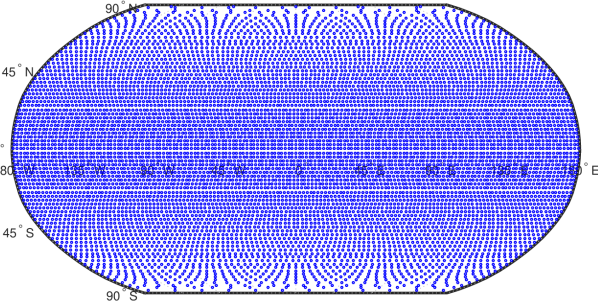
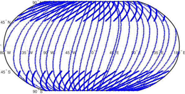
Figure 1: Reuter grid with 8514 points (left) and scattered grid with 8500 points (right).

4.3 Noise generation

For our various scenarios, we get our noisy data if we add white noise to our data values or we add coloured noise that is obtained by an autoregression process. Additionally, we test some local noise.

4.3.1 White noise scenario

For white noise, we add Gaussian noise corresponding to a certain noise-to-singal ratio N2S to the particular value of each datum, that means we get our noisy data by

$$y_{i}^{\varepsilon}=(1+\mathrm{N2S}\cdot\epsilon_{i})y_{i}=\mathrm{N2S}\cdot y_{i}\epsilon_{i}+y_{i},\quad i=1,\dots,l,$$ (32)

where $y_{i}$ are the components of $\boldsymbol{y}$ and $\epsilon_{i}\sim\mathcal{N}(0,1)$, that means every $\epsilon_{i}$ is a standard normally distributed random variable.

4.3.2 Coloured noise scenario

Since our scattered grid tries to imitate tracks of satellites, we can assume that we have a chronology of the data points for each track. To obtain some sort of coloured noise, we use an autoregression process of order $1$ (briefly: AR(1)-process, see [6]) with whom we simulate correlated noise.

A stochastic process $\{\epsilon_{i},\,i\in\mathbb{Z}\}$ is called an autoregressive process of order $1$, if $\epsilon_{i}=\alpha\epsilon_{i-1}+\varepsilon_{i},\ \left|\alpha\right|<1$, where $\varepsilon_{i}\sim\mathcal{N}(0,1)$. In the case of our simulation, we start with $\epsilon_{1}\sim\mathcal{N}(0,1)$ and run the recursion for a fixed $\alpha\in(-1,1)$, which we determined at random.

For each track of the scattered grid, we apply this autoregression process (for the tracks, see Fig. 2) and obtain $y_{i}^{\varepsilon}$ as in (32) using the $\epsilon_{i}$ from above.

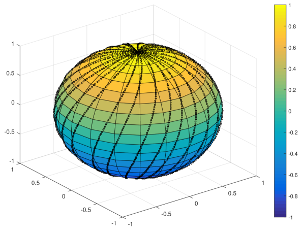
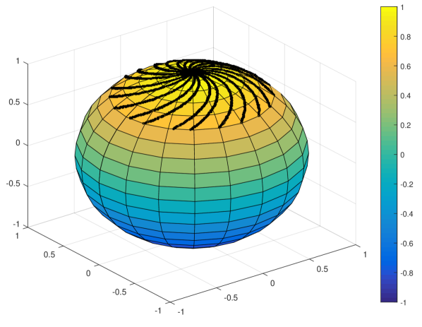
Figure 2: The track sets of the scattered grid (left and right). For the South pole, we have an analogous point distribution.

4.3.3 Local noise scenario

For the local noise, we choose a certain area and add white noise with an $\mathrm{N2S}=5\%$ relative to the particular value to each data point. To the values of the remaining data points we add white noise with an $\mathrm{N2S}=1\%$. We choose this area as illustrated in Fig. 3. The choice of this area is a very rough approximation of the domain of the South Atlantic Anomaly, where a dip in the Earth’s magnetic field exists (see e.g. [17]). Since only a few points of our grid would have been in the actual domain, we extended the area towards the South pole.

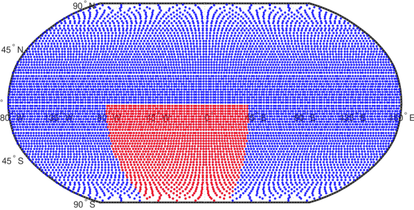
Figure 3: Reuter grid (left) and scattered grid (right). The values of the data points in the red area contain an N2S of $5\%$ and the values of the data points in the blue area an N2S of $1\%$ for the local noise scenario.

Table 2 shows our different test cases for the RFMP and ROFMP.

height	N2S	noise	grid	shortcut
500km	5%	white	scattered	(500,5,wn,S)
500km	5%	coloured	scattered	(500,5,cn,S)
500km	5%	white	Reuter	(500,5,wn,R)
500km	1%	white	scattered	(500,1,wn,S)
500km	1%	coloured	scattered	(500,1,cn,S)
500km	1%	white	Reuter	(500,1,wn,R)
300km	5%	white	scattered	(300,5,wn,S)
300km	5%	coloured	scattered	(300,5,cn,S)
300km	5%	white	Reuter	(300,5,wn,R)
500km	5%/1%	local	scattered	(500,5,ln,S)
500km	5%/1%	local	Reuter	(500,5,ln,R)

Table 2: Overview of the implemented test cases.

4.4 Regularization parameters

We constructed the admissible values $\lambda_{k}$ for the parameter choice as a monotonically decreasing sequence with 100 values from $\lambda_{1}=1$ to $\lambda_{100}=10^{-14}$ and a logarithmically equal spacing in the following way

$$\lambda_{k}=\lambda_{0}q_{\lambda}^{k},\quad k\in\{1,\dots,100\}.$$ (33)

Here, $\lambda_{0}=1.3849$ and $q_{\lambda}=0.7221$. The test scenarios are chosen such that the parameter range lies between $1$ and $10^{-14}$ and includes the optimal parameter away from the boundaries $\lambda_{1}$ and $\lambda_{100}$. For the choice of the parameters $\lambda_{k}$, we refer to [1, 2].

4.5 Maximal index

Most parameter choice methods either increase the index $k$ until a certain condition is satisfied or minimize a certain function for all regularization parameters $\lambda$, i.e. after our discretization (see (33)) they minimize for all $k$ (see Table 1). For some methods like the quasi-optimality criterion, the values of $k$ have to be constrained by a suitable maximal index $\hat{K}$ which must be chosen such that $k_{\mathrm{opt}}<\hat{K}$. To increase computational efficiency, such a maximal index can be used for other methods as well without changing their performance. As in [1, 2], we define this maximal index by

$$\hat{K}=\max\left\{k\,\big{|}\,\rho(k)<0.5\rho(\infty)\right\},$$ (34)

where $\mathbb{E}\|x_{k}-x_{k}^{\varepsilon}\|^{2}=\varepsilon^{2}\rho^{2}(k)$ is the variance of the regularized solution corresponding to noisy data and $\varepsilon^{2}\rho^{2}(\infty)$ is its largest value. It is well-known that, in the case of white noise, $\rho(k)$ for the Tikhonov-Phillips regularization is generally given by

$$\rho^{2}(k)=\sum_{n}\left(\dfrac{\sigma_{n}}{\sigma_{n}^{2}+\lambda_{k}}\right)^{2}.$$ (35)

Since our singular values occur with a multiplicity of $2n+1$ and we restrict our tests to $n=0,\dots,100$, the sum above in our tests is given by

$$\rho^{2}(k)=\sum_{n=0}^{100}(2n+1)\left(\dfrac{\sigma_{n}}{\sigma_{n}^{2}+\lambda_{k}}\right)^{2}.$$ (36)

For any coloured noise, we use the estimate (cf. [2])

$$\varepsilon^{2}\rho^{2}(k)\approx 2^{-1}\left\|x_{k,1}^{\varepsilon}-x_{k,2}^{\varepsilon}\right\|_{\mathcal{H}}^{2},$$ (37)

with two independent data sets $\boldsymbol{y}_{1}^{\varepsilon}$, $\boldsymbol{y}_{2}^{\varepsilon}$ for the same regularization parameter $\lambda_{k}$. Note that $x_{k,1}^{\varepsilon}$, $x_{k,2}^{\varepsilon}$ are the regularized solutions corresponding to the parameter $\lambda_{k}$ and the noisy data sets $\boldsymbol{y}_{1}^{\varepsilon}$, $\boldsymbol{y}_{2}^{\varepsilon}$.

5 Comparison of the methods

For the error comparison, we compute the inefficiency (see (31)) in each scenario (see Table 2 for an overview) for each parameter choice method and compare the inefficiencies. We generate 32 data sets for each of the eleven scenarios, i.e. we run each algorithm for 352 times for a single regularization parameter. Figs. 4 to 14 show the inefficiencies, collected based on the parameter choice methods. The red middle band in the box is the median and the red $+$ symbol shows outliers. The boxplots of our results are plotted at a logarithmic scale.

5.1 Discrepancy principle (DP)

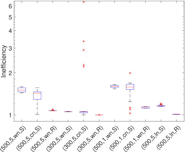
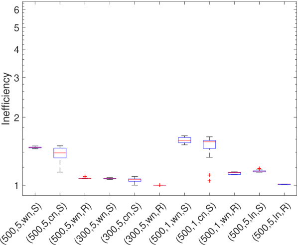
Figure 4: DP for the RFMP (left) and the ROFMP (right).

We can see from Fig. 4 that the DP leads to results which are in the range from good to acceptable in all test cases. It yields better results with a more uniformly distributed grid.

5.2 Transformed discrepancy principle (TDP)

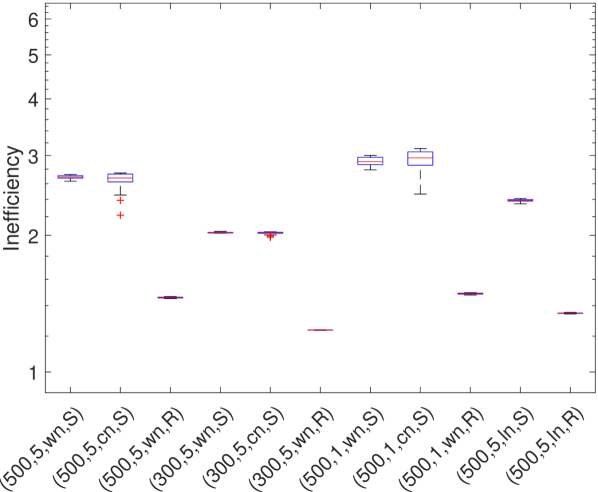
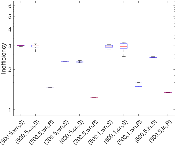
Figure 5: TDP for the RFMP (left) and the ROFMP (right).

The results for the TDP (see Fig. 5) for all test cases are rather poor. We can remark that the results get better with a more uniformly distributed data grid. Furthermore, the coloured noise leads to slightly bigger boxes than the white noise.

5.3 Quasi-optimality criterion (QOC)

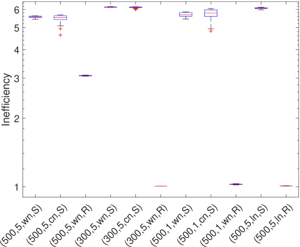
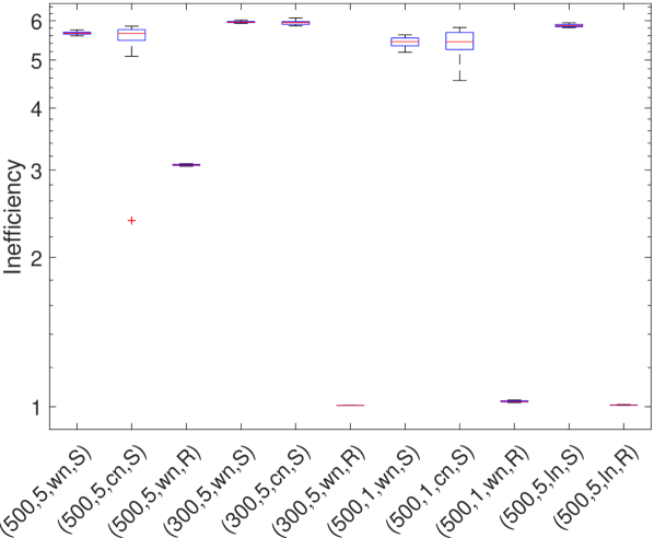
Figure 6: QOC for the RFMP (left) and the ROFMP (right).

In Fig. 6, the inefficiencies of the QOC show that the performance of this method is rather poor. In the case of the Reuter grid, the results reach from good to mediocre in contrast to the scattered grid.

5.4 L-curve method (LC)

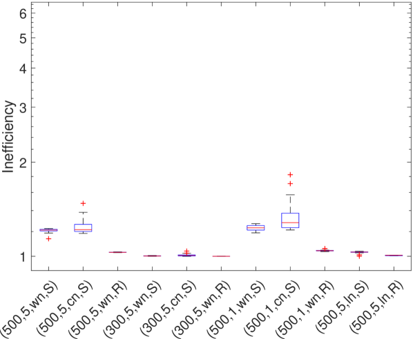
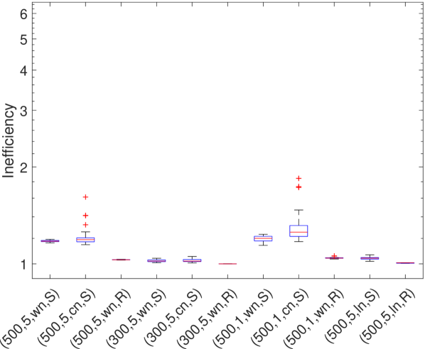
Figure 7: LC for the RFMP (left) and the ROFMP (right).

The LC (see Fig. 7) yields good results in all test cases. We can remark that there are a few outliers and bigger boxes for the test cases with coloured noise and the scattered grid.

5.5 Extrapolated Error method (EEM)

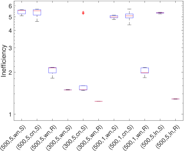
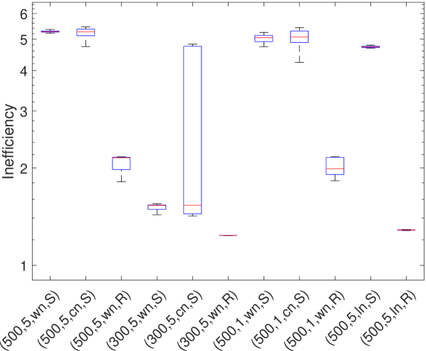
Figure 8: EEM for the RFMP (left) and the ROFMP (right).

The EEM yields acceptable to rather poor results (see Fig. 8). We cannot observe any dependency on the grid or the kind of noise related to the acceptable results. Moreover, in the test case with a height of $300$km and an N2S of $5$% with coloured noise we have some outliers for the RFMP and a large box for the ROFMP.

5.6 Residual method (RM)

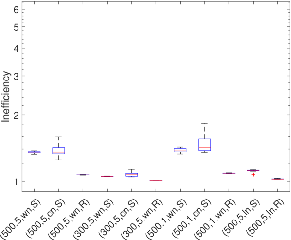
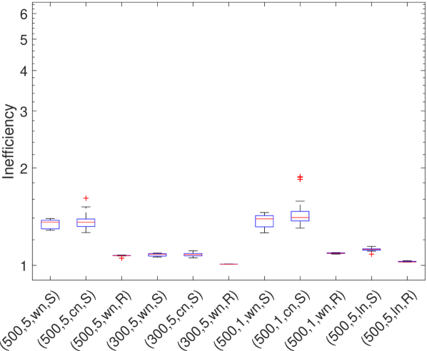
Figure 9: RM for the RFMP (left) and the ROFMP (right).

The results for the RM (see Fig. 9) are good to acceptable in all test cases. We only have a few minor outliers.

5.7 Generalized maximum likelihood (GML)

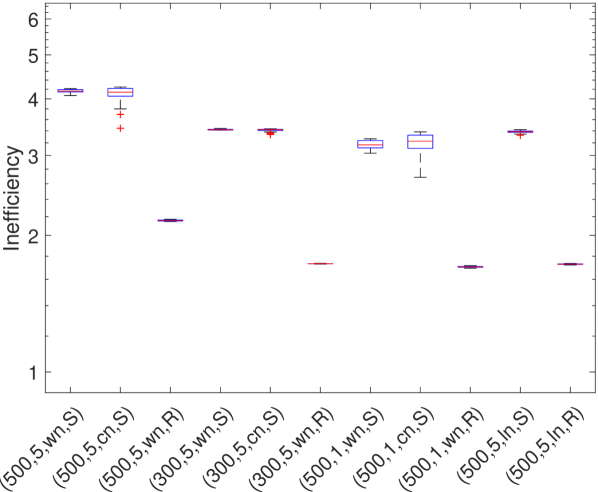
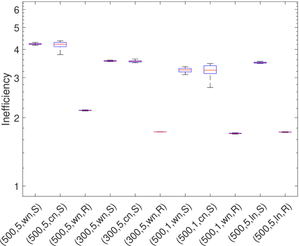
Figure 10: GML for the RFMP (left) and the ROFMP (right).

In Fig. 10, we can see that the GML leads to acceptable results only in the case of the Reuter grid. In all cases of the scattered grid, its performance is rather bad.

5.8 Generalized cross validation (GCV)

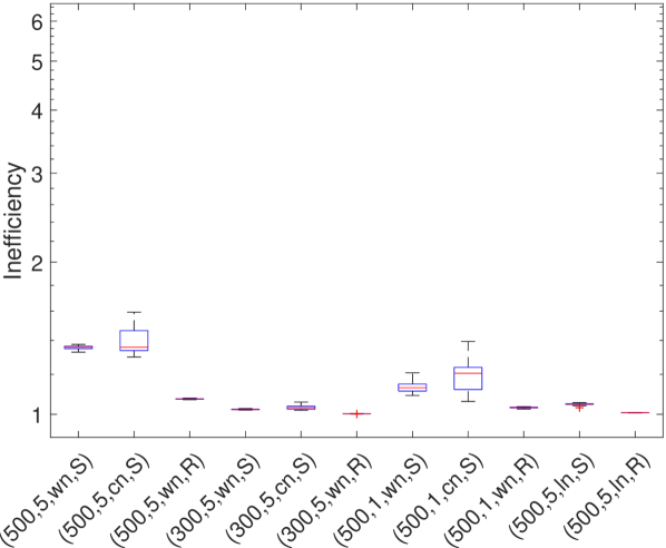
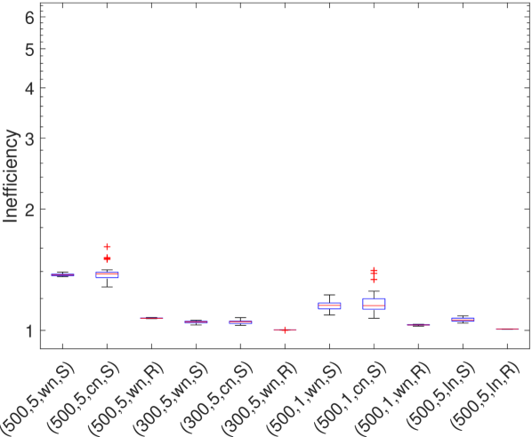
Figure 11: GCV for the RFMP (left) and the ROFMP (right).

From Fig. 11, we can observe that the GCV yields good results in all test cases. We only have, in the case of the ROFMP, some minor outliers. It yields the best results with a more regularly distributed data grid.

5.9 Robust generalized cross validation (RGCV)

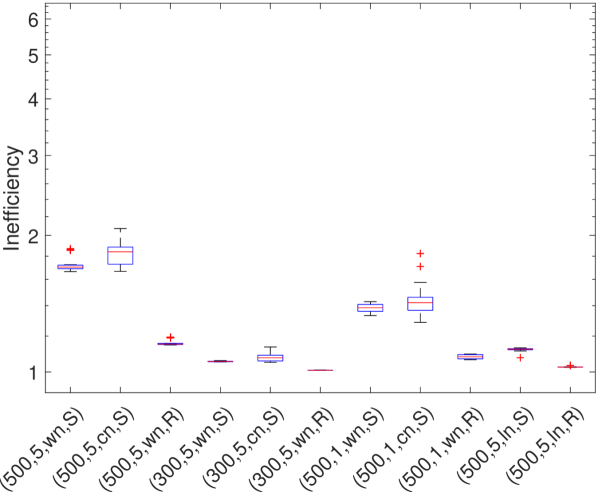
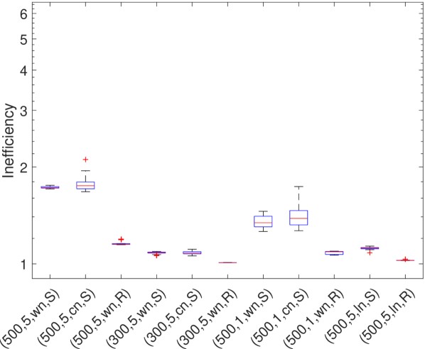
Figure 12: RGCV for the RFMP (left) and the ROFMP (right).

The RGCV yields good to acceptable results (see Fig. 12) which get slightly worse and show a larger variance for a higher N2S or coloured noise scenarios.

5.10 Strong robust generalized cross validation (SRGCV)

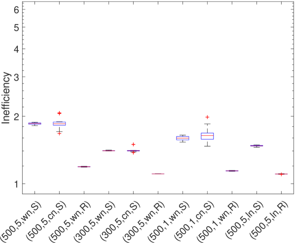
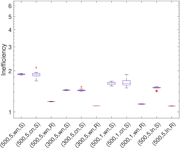
Figure 13: SRGCV for the RFMP (left) and the ROFMP (right).

The SRGCV (see Fig. 13) has good to acceptable results in all the test cases which are a little bit worse than for the RGCV. The Reuter grid leads to good results whereas the scattered grid seems to be more difficult to handle by the method.

5.11 Modified generalized cross validation (MGCV)

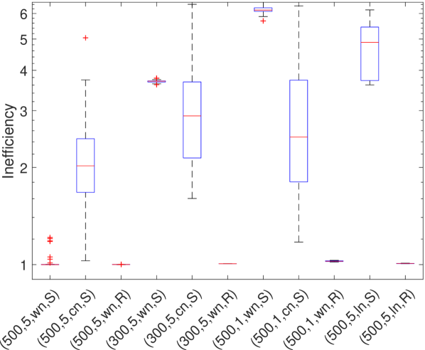
Figure 14: MGCV for the RFMP (left) and the ROFMP (right).

The inefficiencies for the MGCV (see Fig. 14) for the test cases with white noise and the Reuter grid are good. In particular, in several of the cases with coloured noise the boxes are so big that they partially do not fit in the figure. Obviously, we get here a very large distribution of the inefficiencies. These cases seem to be very hard to handle for this method.

5.12 Plots of the results

In this section, we show briefly the approximations of the gravitational potential which we obtain by the RFMP and the ROFMP for one typical noisy data set considering a good or a rather poor parameter choice.

For the test case (500km, 5%, coloured noise, scattered grid) with $\alpha=0.54$ for the AR(1)-process, Fig. 15 shows the approximation which we obtain by the RFMP for the optimal regularization parameter $\lambda_{29}$ and the difference to the EGM2008 up to degree $100$. Fig. 16 shows the approximation belonging to the regularization parameter $\lambda_{22}$ which is chosen by the GCV. In Fig. 17, we can see the approximation belonging to the parameter $\lambda_{43}$ which is chosen by the MGCV. We can see that the MGCV chooses the regularization parameter too small and with this choice we obtain a solution which is underregularized. North-South oriented anomalies occur in the reconstruction which appear to be artefacts due to the noise along the simulated satellite tracks. In contrast, the approximation of the potential for the GCV-based parameter is only slightly worse than the result for the optimal parameter.

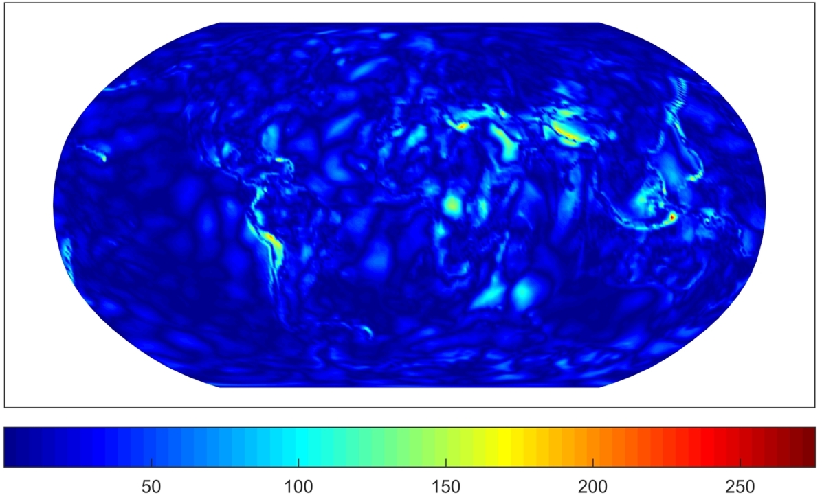
Figure 15: The approximation from the RFMP for the best parameter (left) and the difference to the EGM2008 up to degree $100$ (right). Values in $\mathrm{m^{2}/s^{2}}$.

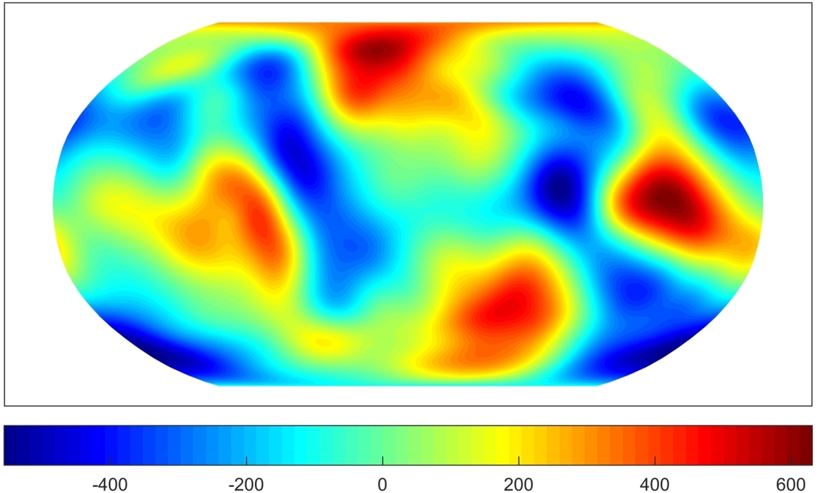
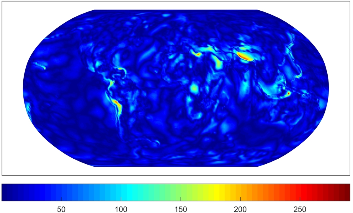
Figure 16: The approximation from the RFMP for the parameter chosen by the GCV (left) and the difference to the EGM2008 up to degree $100$ (right). Values in $\mathrm{m^{2}/s^{2}}$. The inefficiency amounts to $1.16$.

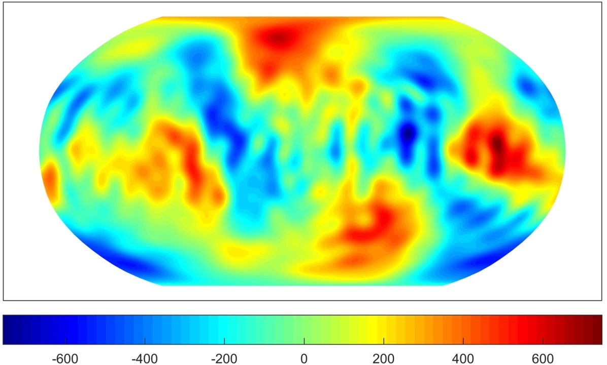
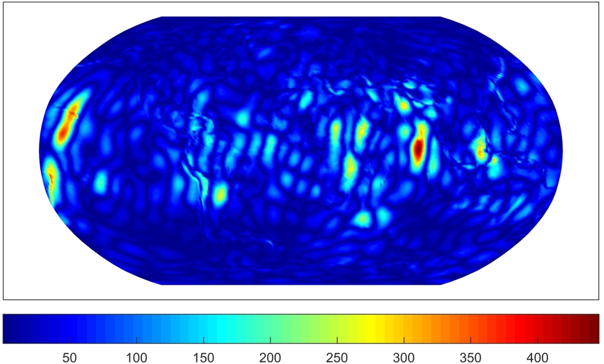
Figure 17: The approximation from the RFMP for the parameter chosen by the MGCV (left) and the difference to the EGM2008 up to degree $100$ (right). Values in $\mathrm{m^{2}/s^{2}}$. The inefficiency amounts to $2.29$.

Furthermore, we show the same test case as above but with the approximation from the ROFMP with $\alpha=0.56$ in the AR(1)-process. Fig. 18 shows the approximation for the optimal parameter $\lambda_{29}$ and the difference to EGM2008. In Fig. 19, we see the approximation which belongs to the parameter $\lambda_{22}$ which is chosen by the GCV. Fig. 20 shows the approximation with the regularization parameter $\lambda_{9}$ which is chosen by the GML.

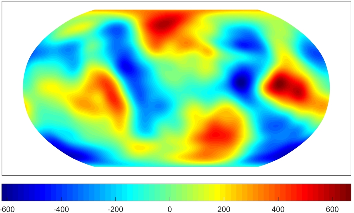
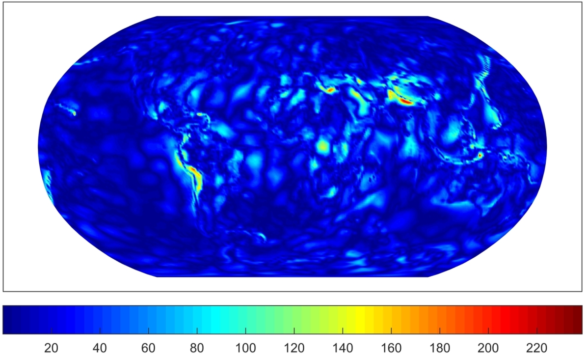
Figure 18: The approximation from the ROFMP for the best parameter (left) and the difference to the EGM2008 up to degree $100$ (right). Values in $\mathrm{m^{2}/s^{2}}$.

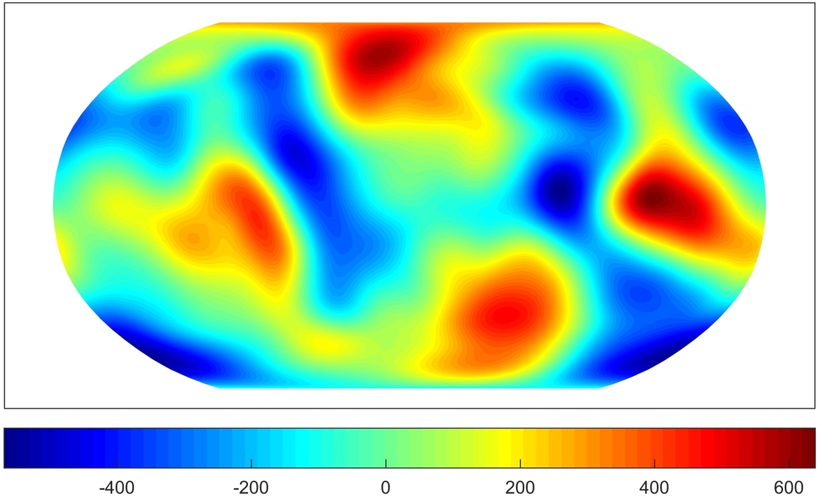
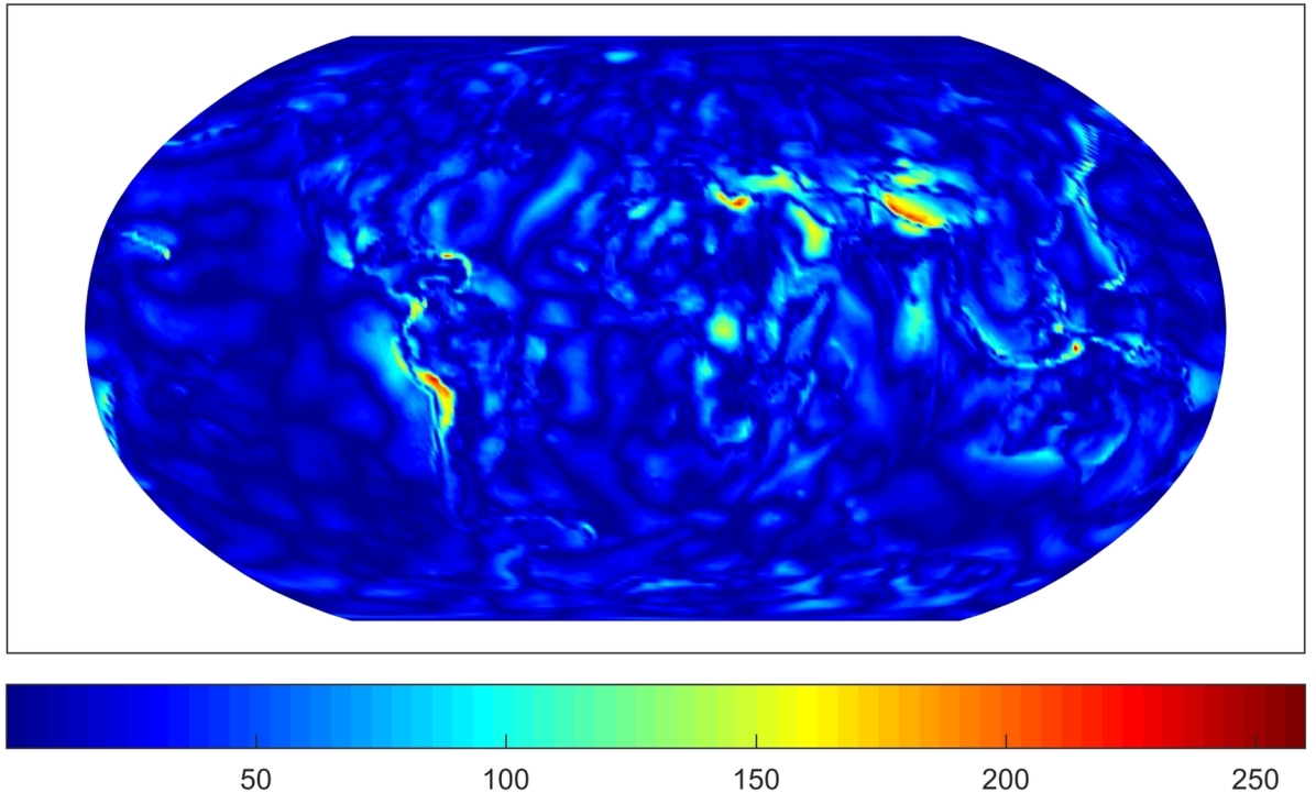
Figure 19: The approximation from the ROFMP for the parameter chosen by the GCV (left) and the difference to the EGM2008 up to degree $100$ (right). Values in $\mathrm{m^{2}/s^{2}}$. The inefficiency amounts to $1.14$.

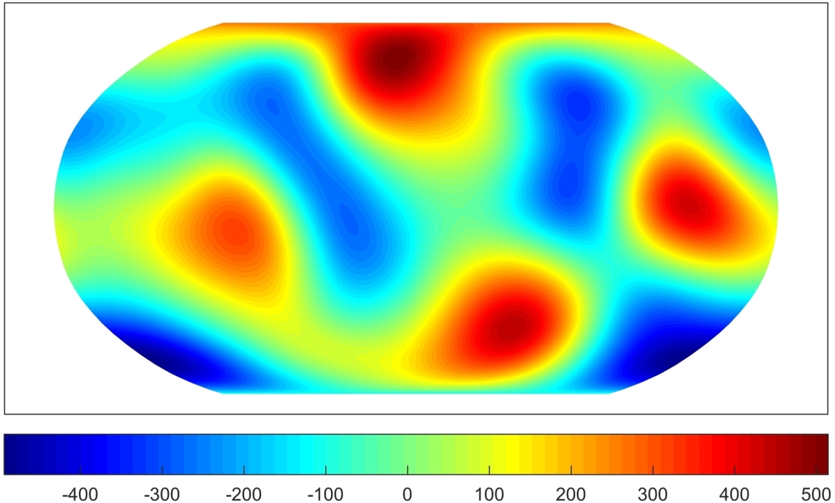
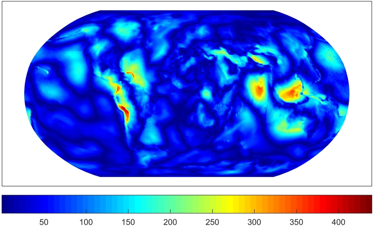
Figure 20: The approximation from the ROFMP for the parameter chosen by the GML (left) and the difference to the EGM2008 up to degree $100$ (right). Values in $\mathrm{m^{2}/s^{2}}$. The inefficiency amounts to $3.03$.

Here, the GML chooses a regularization parameter which is too large that means our approximation is overregularized. We get less information and details about the gravitational potential. Essential details such as signals due to the Andes or the region around Indonesia occur in the difference plot – much stronglier than for the other examples. Again the parameter choice of the GCV yields a good approximation for the gravitational potential.

Finally, Figs. 21 and 22 show the difference $\|x-x_{k}^{\varepsilon}\|_{\mathrm{L}^{2}(\Omega)}$ between the original solution (i.e. EGM2008 up to degree $100$) and the approximation $x_{k}^{\varepsilon}$ obtained for the different regularization parameters which were chosen by the considered strategies. The horizontal axis states the index $k$ of the regularization parameter $\lambda_{k}$. The plots refer to the same scenario as Figures 15 to 20. The arrows show the parameters which are chosen by the methods. The diagrams confirm our observations that the GCV and the LC yield parameters which are closest to the (theoretical) optimal parameter. We obtain almost equally good results for the DP, the RM and the RGCV.

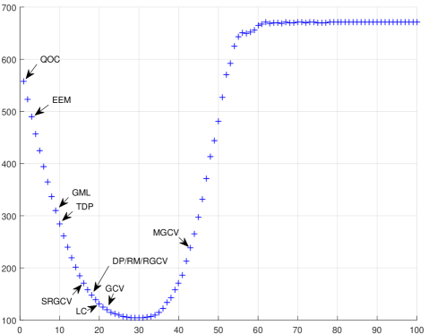
Figure 21: The horizontal axis states the index $k$ of the regularization parameter and the vertical axis shows $\|x-x_{k}^{\varepsilon}\|_{\mathrm{L}^{2}(\Omega)}$ for the RFMP.

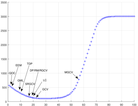
Figure 22: The horizontal axis states the index $k$ of the regularization parameter and the vertical axis shows $\|x-x_{k}^{\varepsilon}\|_{\mathrm{L}^{2}(\Omega)}$ for the ROFMP.

6 Conclusion and outlook

We tested parameter choice methods for the regularized (orthogonal) functional matching pursuit (RFMP/ROFMP). For the evaluation of the parameter choice methods, we constructed eleven different test cases with different satellite heights, data grids, noise types and noise-to-signal ratios (see Table 2) for the RFMP and ROFMP. For each test case, we generated $32$ noisy data sets. Altogether we ran each algorithm for $352$ data sets and for each data set for $100$ different regularization parameters, that means each algorithm was applied 35200 times.

Our study shows that the GCV, the LC, the RM, the RGCV and the SRGCV yield the best results in all test cases. The DP provides good to acceptable results. The performance of the QOC seriously depends on the data grid, that means a less regularly distributed grid does not lead to good results. In our experiments, the QOC had good results with the Reuter grid. The MGCV also obtains both good and rather poor results in dependency on the grid and kind of noise we used. Here, the irregularly distributed scattered grid and the coloured noise did not yield good results. At last, the TDP, the EEM and the GML did not always lead to good results in our test cases.

We want to remark that in average our results were better than in [1] and [2] for all methods. Some possible reasons for that can be: the coloured noise in our test cases was different and maybe easier to handle for the methods than in the two papers, because we only had an AR(1)-process. There is a further difference to the other cases in relation to the problem itself. Here we had a data grid given which corresponds to a spatial discretization of the problem. Furthermore, the RFMP and the ROFMP are iterative methods and use stopping criteria which are also some kind of regularization. Since we stop the algorithm at a certain point we do not obtain the approximation of the potential in the limit. For these reasons, the outcomes of our experiments and of those in [1, 2] are not really comparable.

The purpose of this paper is to provide a first guideline for the parameter choice for the RFMP and the ROFMP. Certainly, further experiments should be designed in the future. Maybe, the distribution of our regularization parameters $\lambda_{k}$ could be improved such that the relevant parameters themselves are not too wide apart. Perhaps, the interval from $1$ to $10^{-14}$ should be chosen smaller such that the parameters are closer together.

Future changes in the implementation could also be the use of other stopping criteria for the RFMP. Furthermore, an enhancement could be the extension of the dictionary to localized trial functions. In addition, the generation of the coloured noise can, for example, use an $AR(k)$-process for $k>1$ or completely different types of noise can be considered. Finally, we can test other tuning parameters for the methods as far as these are required. Besides, it is possible that the performance of the investigated parameter choice methods in the RFMP/ROFMP depends on the considered inverse problem.

References

- [1] F. Bauer, M. Gutting, and M. A. Lukas. Evaluation of parameter choice methods for the regularization of ill-posed problems in geomathematics. In W. Freeden, M. Nashed, and T. Sonar, editors, Handbook of Geomathematics, pages 1713–1774. Springer, Berlin, Heidelberg, 2nd edition, 2014.
- [2] F. Bauer and M. A. Lukas. Comparing parameter choice methods for regularization of ill-posed problems. Math. Comput. Simul., 81:1795–1841, 2011.
- [3] F. Bauer and P. Mathé. Parameter choice methods using minimization schemes. J. Complexity, 27:68–85, 2011.
- [4] C. Brezinski, G. Rodriguez, and S. Seatzu. Error estimates for linear systems with applications to regularization. Numer. Algorithms, 49:85–104, 2008.
- [5] C. Brezinski, G. Rodriguez, and S. Seatzu. Error estimates for the regularization of least squares problems. Numer. Algorithms, 51:61–76, 2009.
- [6] P. J. Brockwell and R. A. Davis. Introduction to Time Series and Forecasting. Springer, New York, 2nd edition, 2002.
- [7] D. J. Cummins, T. G. Filloon, and D. Nychka. Confidence intervals for nonparametric curve estimates: toward more uniform pointwise coverage. J. Am. Stat. Assoc., 96:233–246, 2001.
- [8] M. R. Drinkwater, R. Haagmans, D. Muzi, A. Popescu, R. Floberghagen, M. Kern, and M. Fehringer. The GOCE gravity mission: ESA’s first core explorer. In Proceedings of the 3rd GOCE User Workshop, volume SP-627, pages 1–8. ESA Special Publication, Frascati, 2006.
- [9] D. Fischer. Sparse Regularization of a Joint Inversion of Gravitational Data and Normal Mode Anomalies. PhD thesis, Geomathematics Group, Department of Mathematics, University of Siegen, Verlag Dr. Hut, Munich, 2011.
- [10] D. Fischer and V. Michel. Sparse regularization of inverse gravimetry—case study: spatial and temporal mass variations in South America. Inverse Probl., 28:065012, 2012.
- [11] W. Freeden, T. Gervens, and M. Schreiner. Constructive Approximation on the Sphere. With Applications to Geomathematics. Oxford University Press, Oxford, 1998.
- [12] W. Freeden and M. Gutting. Special Functions of Mathematical (Geo-) physics. Birkhäuser, Basel, 2013.
- [13] W. Freeden and V. Michel. Multiscale Potential Theory. With Applications to Geoscience. Birkhäuser, Boston, 2004.
- [14] P. C. Hansen. Analysis of discrete ill-posed problems by means of the L-curve. SIAM Rev., 34:561–580, 1992.
- [15] P. C. Hansen. Rank-deficient and Discrete Ill-posed Problems. Numerical Aspects of Linear Inversion. SIAM, Philadelphia, 1998.
- [16] P. C. Hansen and D. P. O’Leary. The use of the L-curve in the regularization of discrete ill-posed problems. SIAM J. Sci. Comput., 14:1487–1503, 1993.
- [17] J. Heirtzler. The future of the South Atlantic anomaly and implications for radiation damage in space. J. Atmos. Sol.-Terr. Phy., 64:1701–1708, 2002.
- [18] K. H. Ilk, J. Flury, R. Rummel, P. Schwintzer, W. Bosch, C. Haas, J. Schröter, D. Stammer, W. Zahel, H. Schmeling, D. Wolf, J. Riegger, A. Bardossy, and A. Güntner. Mass transport and mass distribution in the Earth system:Contribution of the New Generation of Satellite Gravity and Altimetry Missions to Geosciences. Proposal for a German priority research program, 1st edition, GOCE-Projektbüro TU München, GeoForschungsZentrum Potsdam, 2004. http://gfzpublic.gfz-potsdam.de/pubman/faces/viewItemOverviewPage.jsp?itemId=escidoc:231104:1, last access: 10 October 2016.
- [19] J. Kusche, V. Klemann, and N. Sneeuw. Mass distribution and mass transport in the Earth system: recent scientific progress due to interdisciplinary research. Surv. Geophys., 35:1243–1249, 2014.
- [20] M. A. Lukas. Robust generalized cross-validation for choosing the regularization parameter. Inverse Probl., 22:1883–1902, 2006.
- [21] M. A. Lukas. Strong robust generalized cross-validation for choosing the regularization parameter. Inverse Probl., 24:034006, 2008.
- [22] S. G. Mallat and Z. Zhang. Matching pursuits with time-frequency dictionaries. IEEE T. Signal Proces., 41:3397–3415, 1993.
- [23] V. Michel. Lectures on Constructive Approximation – Fourier, Spline, and Wavelet Methods on the Real Line, the Sphere, and the Ball. Birkhäuser, New York, 2013.
- [24] V. Michel. RFMP – an iterative best basis algorithm for inverse problems in the geosciences. In W. Freeden, M. Nashed, and T. Sonar, editors, Handbook of Geomathematics, pages 2121–2147. Springer, Berlin, Heidelberg, 2nd edition, 2015.
- [25] V. Michel and S. Orzlowski. On the convergence theorem for the Regularized Functional Matching Pursuit (RFMP) algorithm. Preprint, Siegen Preprints on Geomathematics, Issue 13, 2016.
- [26] V. Michel and R. Telschow. A non-linear approximation method on the sphere. GEM. Int. J. Geomath., 5:195–224, 2014.
- [27] V. Michel and R. Telschow. The regularized orthogonal functional matching pursuit for ill-posed inverse problems. SIAM J. Numer. Anal., 54:262–287, 2016.
- [28] V. A. Morozov. On the solution of functional equations by the method of regularization. Sov. Math. Dokl., 7:414–417, 1966.
- [29] V. A. Morozov. Methods for Solving Incorrectly Posed Problems. Springer, New York, 1984.
- [30] C. Müller. Spherical Harmonics. Springer, Berlin, Heidelberg, 1966.
- [31] R. Pail, H. Goiginger, W.-D. Schuh, E. Höck, J. M. Brockmann, T. Fecher, T. Gruber, T. Mayer-Gürr, J. Kusche, A. Jäggi, and D. Rieser. Combined satellite gravity field model GOCO01S derived from GOCE and GRACE. Geophys. Res. Lett., 37:L20314, 2010.
- [32] Y. C. Pati, R. Rezaiifar, and P. S. Krishnaprasad. Orthogonal matching pursuit: recursive function approximation with applications to wavelet decomposition. In Asimolar Conference on Signals, Systems and Computers, volume 1 of IEEE Conference Publications, pages 40–44, 1993.
- [33] N. K. Pavlis, S. A. Holmes, S. C. Kenyon, and J. K. Factor. The development and evaluation of the Earth Gravitational Model 2008 (EGM2008). J. Geophys. Res.-Sol. Ea., 117, 2012.
- [34] D. Phillips. A technique for the numerical solution of certain integral equations of the first kind. J. Assoc. Comput. Mach., 9:84–97, 1962.
- [35] T. Raus. An a posteriori choice of the regularization parameter in case of approximately given error bound of data. In A. Pedas, editor, Collocation and Projection Methods for Integral Equations and Boundary Value Problems, pages 73–87. Tartu: Tartu University, 1990.
- [36] T. Raus. About regularization parameter choice in case of approximately given error bounds of data. In G. Vainikko, editor, Methods for Solution of Integral Equations and Ill-posed Problems, pages 77–89. Tartu: Tartu University, 1992.
- [37] C. Reigber, G. Balmino, P. Schwintzer, R. Biancale, A. Bode, J.-M. Lemoine, R. König, S. Loyer, H. Neumayer, J.-C. Marty, F. Barthelmes, F. Perosanz, and S. Y. Zhu. New global gravity field models from selected CHAMP data sets. In First CHAMP Mission Results for Gravity, Magnetic and Atmospheric Studies, pages 120–127. Springer, Berlin, Heidelberg, 2003.
- [38] R. Reuter. Integralformeln der Einheitssphäre und harmonische Splinefunktionen. PhD thesis, RWTH Aachen, 1982.
- [39] T. Robinson and R. Moyeed. Making robust the cross-validatory choice of smoothing parameter in spline smoothing regression. Commun. Stat. Theory Methods, 18:523–539, 1989.
- [40] F. Schneider. Inverse Problems in Satellite Geodesy and Their Approximation in Satellite Gradiometry. PhD thesis, Geomathematics Group, Department of Mathematics, University of Kaiserslautern, 1997.
- [41] B. D. Tapley, S. Bettadpur, M. Watkins, and C. Reigber. The gravity recovery and climate experiment: mission overview and early results. Geophys. Res. Lett., 31, 2004. L09607.
- [42] R. Telschow. An Orthogonal Matching Pursuit for the Regularization of Spherical Inverse Problems. PhD thesis, Geomathematics Group, Department of Mathematics, University of Siegen, 2014, Verlag Dr. Hut, Munich, 2015.
- [43] A. Tikhonov and V. Y. Arsenin. Solutions of Ill-posed Problems. Wiley, New York, 1977.
- [44] A. Tikhonov and V. Glasko. Use of the regularization method in non-linear problems. USSR Comput. Math. Math. Phys., 5:93–107, 1967.
- [45] P. Vincent and Y. Bengio. Kernel matching pursuit. Machine Learning, 48:165–187, 2002.
- [46] R. Vio, P. Ma, W. Zhong, J. Nagy, L. Tenorio, and W. Wamsteker. Estimation of regularization parameters in multiple-image deblurring. Astron. Astrophys., 423:1179–1186, 2004.
- [47] G. Wahba. Practical approximate solutions to linear operator equations when the data are noisy. SIAM J. Numer. Anal., 14:651–667, 1977.
- [48] G. Wahba. A comparison of GCV and GML for choosing the smoothing parameter in the generalized spline smoothing problem. Ann. Stat., 13:1378–1402, 1985.