Low Rank Approximation with Entrywise $\ell_{1}$-Norm Error

We study the $\ell_{1}$-low rank approximation problem, where for a given $n\times d$ matrix $A$ and approximation factor $\alpha\geq 1$, the goal is to output a rank-$k$ matrix $\widehat{A}$ for which

$$\|A-\widehat{A}\|_{1}\leq\alpha\cdot\min_{\textrm{rank-}k\textrm{ matrices}\leavevmode\nobreak\ A^{\prime}}\|A-A^{\prime}\|_{1},$$

where for an $n\times d$ matrix $C$, we let $\|C\|_{1}=\sum_{i=1}^{n}\sum_{j=1}^{d}|C_{i,j}|$. This error measure is known to be more robust than the Frobenius norm in the presence of outliers and is indicated in models where Gaussian assumptions on the noise may not apply. The problem was shown to be NP-hard by Gillis and Vavasis and a number of heuristics have been proposed. It was asked in multiple places if there are any approximation algorithms.

We give the first provable approximation algorithms for $\ell_{1}$-low rank approximation, showing that it is possible to achieve approximation factor $\alpha=(\log d)\cdot\operatorname{poly}(k)$ in $\operatorname{nnz}(A)+(n+d)\operatorname{poly}(k)$ time, where $\operatorname{nnz}(A)$ denotes the number of non-zero entries of $A$. If $k$ is constant, we further improve the approximation ratio to $O(1)$ with a $\operatorname{poly}(nd)$-time algorithm. Under the Exponential Time Hypothesis, we show there is no $\operatorname{poly}(nd)$-time algorithm achieving a $(1+\frac{1}{\log^{1+\gamma}(nd)})$-approximation, for $\gamma>0$ an arbitrarily small constant, even when $k=1$.

We give a number of additional results for $\ell_{1}$-low rank approximation: nearly tight upper and lower bounds for column subset selection, CUR decompositions, extensions to low rank approximation with respect to $\ell_{p}$-norms for $1\leq p<2$ and earthmover distance, low-communication distributed protocols and low-memory streaming algorithms, algorithms with limited randomness, and bicriteria algorithms. We also give a preliminary empirical evaluation.

1 Introduction

Two well-studied problems in numerical linear algebra are regression and low rank approximation. In regression, one is given an $n\times d$ matrix $A$, and an $n\times 1$ vector $b$, and one seeks an $x\in\mathbb{R}^{d}$ which minimizes $\|Ax-b\|$ under some norm. For example, for least squares regression one minimizes $\|Ax-b\|_{2}$. In low rank approximation, one is given an $n\times d$ matrix $A$, and one seeks a rank-$k$ matrix $\widehat{A}$ which minimizes $\|A-\widehat{A}\|$ under some norm. For example, in Frobenius norm low rank approximation, one minimizes $\|A-\widehat{A}\|_{F}=\left(\sum_{i,j}(A_{i,j}-\widehat{A}_{i,j})^{2}\right)^{1/2}$. Algorithms for regression are often used as subroutines for low rank approximation. Indeed, one of the main insights of [DMM06b, DMM06a, Sar06, DMM08, CW09] was to use results for generalized least squares regression for Frobenius norm low rank approximation. Algorithms for $\ell_{1}$-regression, in which one minimizes $\|Ax-b\|_{1}=\sum_{i}|(Ax)_{i}-b_{i}|$, were also used [BD13, SW11] to fit a set of points to a hyperplane, which is a special case of entrywise $\ell_{1}$-low rank approximation, the more general problem being to find a rank-$k$ matrix $\widehat{A}$ minimizing $\sum_{i,j}|A_{i,j}-\widehat{A}_{i,j}|$.

Randomization and approximation were introduced to significantly speed up algorithms for these problems, resulting in algorithms achieving relative error approximation with high probability. Such algorithms are based on sketching and sampling techniques; we refer to [Woo14b] for a survey. For least squares regression, a sequence of work [Sar06, CW13, MM13, NN13, LMP13, BDN15, Coh16] shows how to achieve algorithms running in $\operatorname{nnz}(A)+\operatorname{poly}(d)$ time. For Frobenius norm low rank approximation, using the advances for regression this resulted in $\operatorname{nnz}(A)+(n+d)\operatorname{poly}(k)$ time algorithms. For $\ell_{1}$-regression, sketching and sampling-based methods [Cla05, SW11, CDMI⁺13, CW13, MM13, LMP13, WZ13, CW15b, CP15] led to an $\operatorname{nnz}(A)+\operatorname{poly}(d)$ time algorithm.

Just like Frobenius norm low rank approximation is the analogue of least squares regression, entrywise $\ell_{1}$-low rank approximation is the analogue of $\ell_{1}$-regression. Despite this analogy, no non-trivial upper bounds with provable guarantees are known for $\ell_{1}$-low rank approximation. Unlike Frobenius norm low rank approximation, which can be solved exactly using the singular value decomposition, no such algorithm or closed-form solution is known for $\ell_{1}$-low rank approximation. Moreover, the problem was recently shown to be NP-hard [GV15]. A major open question is whether there exist approximation algorithms, sketching-based or otherwise, for $\ell_{1}$-low rank approximation. Indeed, the question of obtaining betters algorithms was posed in section 6 of [GV15], in [Exc13], and as the second part of open question 2 in [Woo14b], among other places. The earlier question of NP-hardness was posed in Section 1.4 of [KV09], for which the question of obtaining approximation algorithms is a natural followup. The goal of our work is to answer this question.

We now formally define the $\ell_{1}$-low rank approximation problem: we are given an $n\times d$ matrix $A$ and approximation factor $\alpha\geq 1$, and we would like, with large constant probability, to output a rank-$k$ matrix $\widehat{A}$ for which

$$\|A-\widehat{A}\|_{1}\leq\alpha\cdot\min_{\textrm{rank-}k\textrm{ matrices\leavevmode\nobreak\ }A^{\prime}}\|A-A^{\prime}\|_{1},$$

where for an $n\times d$ matrix $C$, we let $\|C\|_{1}=\sum_{i=1}^{n}\sum_{j=1}^{d}|C_{i,j}|$. This notion of low rank approximation has been proposed as a more robust alternative to Frobenius norm low rank approximation [KK03, KK05, KLC⁺15, Kwa08, ZLS⁺12, BJ12, BD13, BDB13, MXZZ13, MKP13, MKP14, MKCP16, PK16], and is sometimes referred to as $\ell_{1}$-matrix factorization or robust PCA. $\ell_{1}$-low rank approximation gives improved results over Frobenius norm low rank approximation since outliers are less exaggerated, as one does not square their contribution in the objective. The outlier values are often erroneous values that are far away from the nominal data, appear only a few times in the data matrix, and would not appear again under normal system operation. These works also argue $\ell_{1}$-low rank approximation can better handle missing data, is appropriate in noise models for which the noise is not Gaussian, e.g., it produces the maximum likelihood estimator for Laplacian noise [Gao08, KAC⁺08, VT01], and can be used in image processing to prevent image occlusion [YZD12].

To see that $\ell_{1}$-low rank approximation and Frobenius norm low rank approximation can give very different results, consider the $n\times n$ matrix $A=\left[\begin{smallmatrix}n&0\\ 0&B\end{smallmatrix}\right]$, where $B$ is any $(n-1)\times(n-1)$ matrix with $\|B\|_{F}<n$. The best rank-$1$ approximation with Frobenius norm error is given by $\widehat{A}=n\cdot e_{1}e_{1}^{\top}$, where $e_{1}$ is the first standard unit vector. Here $\widehat{A}$ ignores all but the first row and column of $A$, which may be undesirable in the case that this row and column represent an outlier. Note $\|A-\widehat{A}\|_{1}=\|B\|_{1}$. If, for example, $B$ is the all $1$s matrix, then $\widehat{A}=[0,0;0,B]$ is a rank-$1$ approximation for which $\|A-\widehat{A}\|_{1}=n$, and therefore this solution is a much better solution to the $\ell_{1}$-low rank approximation problem than $n\cdot e_{1}e_{1}^{\top}$, for which $\|A-n\cdot e_{1}e_{1}^{\top}\|_{1}=(n-1)^{2}.$

Despite the advantages of $\ell_{1}$-low rank approximation, its main disadvantage is its computationally intractability. It is not rotationally invariant and most tools for Frobenius low rank approximation do not apply. To the best of our knowledge, all previous works only provide heuristics. We provide hard instances for previous work in Section L, showing these algorithms at best give a $\operatorname{poly}(nd)$-approximation (though even this is not shown in these works). We also mention why a related objective function, robust PCA [WGR⁺09, CLMW11, NNS⁺14, NYH14, CHD16, ZZL15], does not give a provable approximation factor for $\ell_{1}$-low rank approximation. Using that for an $n\times d$ matrix $C$, $\|C\|_{F}\leq\|C\|_{1}\leq\sqrt{nd}\|C\|_{F}$, a Frobenius norm low rank approximation gives a $\sqrt{nd}$ approximation for $\ell_{1}$-low rank approximation. A bit better is to use algorithms for low rank approximation with respect to the sum of distances, i.e., to find a rank-$k$ matrix $\widehat{A}$ minimizing $\|A-\widehat{A}\|_{1,2}$, where for an $n\times d$ matrix $C$, $\|C\|_{1,2}=\sum_{i=1}^{n}\|C_{i}\|_{2}$, where $C_{i}$ is the $i$-th row of $C$. A sequence of work [DV07, FMSW10, FL11, SV12, CW15a] shows how to obtain an $O(1)$-approximation to this problem in $\operatorname{nnz}(A)+(n+d)\operatorname{poly}(k)+\exp(k)$ time, and using that $\|C\|_{1,2}\leq\|C\|_{1}\leq\sqrt{d}\|C\|_{1,2}$ results in an $O(\sqrt{d})$-approximation.

There are also many variants of Frobenius norm low rank approximation for which nothing is known for $\ell_{1}$-low rank approximation, such as column subset selection and CUR decompositions, distributed and streaming algorithms, algorithms with limited randomness, and bicriteria algorithms. Other interesting questions include low rank approximation for related norms, such as $\ell_{p}$-low rank approximation in which one seeks a rank-$k$ matrix $\widehat{A}$ minimizing $\sum_{i=1}^{n}\sum_{j=1}^{d}(A_{i,j}-\widehat{A}_{i,j})^{p}$. Note for $1\leq p<2$ these are also more robust than the SVD.

1.1 Our Results

We give the first efficient algorithms for $\ell_{1}$-low rank approximation with provable approximation guarantees. By symmetry of the problem, we can assume $d\leq n$. We first give an algorithm which runs in $O(\operatorname{nnz}(A))+n\cdot\operatorname{poly}(k)$ time and solves the $\ell_{1}$-low rank approximation problem with approximation factor $(\log d)\cdot\operatorname{poly}(k)$. This is an exponential improvement over the previous approximation factor of $O(\sqrt{d})$, provided $k$ is not too large, and is polynomial time for every $k$. Moreover, provided $\operatorname{nnz}(A)\geq n\cdot\operatorname{poly}(k)$, our time is optimal up to a constant factor as any relative error algorithm must spend $\operatorname{nnz}(A)$ time. We also give a hard instance for our algorithm ruling out $\frac{\log d}{k\log k}+k^{1/2-\gamma}$ approximation for arbitrarily small constant $\gamma>0$, and hard instances for a general class of algorithms based on linear sketches, ruling out $k^{1/2-\gamma}$ approximation.

Via a different algorithm, we show how to achieve an $\widetilde{O}(k)$-approximation factor in
$\operatorname{poly}(n)d^{\widetilde{O}(k)}2^{\widetilde{O}(k^{2})}$ time. This is useful for constant $k$, for which it gives an $O(1)$-approximation in $\operatorname{poly}(n)$ time, improving the $O(\log d)$-approximation for constant $k$ of our earlier algorithm. The approximation ratio of this algorithm, although $O(1)$ for constant $k$, depends on $k$. We also show one can find a rank-$2k$ matrix $\widehat{A}$ in $\operatorname{poly}(n)$ time for constant $k$ for which $\|A-\widehat{A}\|_{1}\leq C\min_{\textrm{rank-}k\textrm{ matrices\leavevmode\nobreak\ }A^{\prime}}\|A-A^{\prime}\|_{1}$, where $C>1$ is an absolute constant independent of $k$. We refer to this as a bicriteria algorithm. Finally, one can output a rank-$k$ matrix $\widehat{A}$, instead of a rank-$2k$ matrix $\widehat{A}$, in $\operatorname{poly}(n)$ time with the same absolute constant $C$ approximation factor, under an additional assumption that the entries of $\widehat{A}$ are integers in the range $\{-b,-b+1,\ldots,b\}$ for an integer $b\leq\operatorname{poly}(n)$. Unlike our previous algorithms, this very last algorithm has a bit complexity assumption, and runs in $\operatorname{poly}(b)$ time instead of $\operatorname{poly}(\log(b))$ time.

Under the Exponential Time Hypothesis ($\mathsf{ETH}$), we show there is no $\operatorname{poly}(n)$-time algorithm achieving a $(1+\frac{1}{\log^{1+\gamma}(n)})$-approximation, for $\gamma>0$ an arbitrarily small constant, even when $k=1$. The latter strengthens the NP-hardness result of [GV15].

We also give a number of results for variants of $\ell_{1}$-low rank approximation which are studied for Frobenius norm low rank approximation; prior to our work nothing was known about these problems.

Column Subset Selection and CUR Decomposition: In the column subset selection problem, one seeks a small subset $C$ of columns of $A$ for which there is a matrix $X$ for which $\|CX-A\|$ is small, under some norm. The matrix $CX$ provides a low rank approximation to $A$ which is often more interpretable, since it stores actual columns of $A$, preserves sparsity, etc. These have been extensively studied when the norm is the Frobenius or operator norm (see, e.g., [BMD09, DR10, BDM11] and the references therein). We initiate the study of this problem with respect to the $\ell_{1}$-norm. We first prove an existence result, namely, that there exist matrices $A$ for which any subset $C$ of $\operatorname{poly}(k)$ columns satisfies $\min_{X}\|CX-A\|_{1}\geq k^{1/2-\gamma}\cdot\min_{\textrm{rank-}k\textrm{ matrices\leavevmode\nobreak\ }A^{\prime}}\|A-A^{\prime}\|_{1}$, where $\gamma>0$ is an arbitrarily small constant. This result is in stark contrast to the Frobenius norm for which for every matrix there exist $O(\frac{k}{\epsilon})$ columns for which the approximation factor is $1+\epsilon$. We also show that our bound is nearly optimal in this regime, by showing for every matrix there exists a subset of $O(k\log k)$ columns providing an $O(\sqrt{k\log k})$-approximation. One can find such columns in $\operatorname{poly}(n)d^{O(k\log k)}$ time by enumerating and evaluating the cost of each subset. Although this is exponential in $k$, we show it is possible to find $O(k\log k)$ columns providing a larger $O(k\log k\log d)$-approximation in polynomial time for every $k$.

We extend these results to the CUR decomposition problem (see, e.g., [DMM08, BW14]), in which one seeks a factorization $CUR$ for which $C$ is a subset of columns of $A$, $R$ is a subset of rows of $A$, and $\|CUR-A\|$ is as small as possible. In the case of Frobenius norm, one can choose $O(k/\epsilon)$ columns and rows, have rank$(U)=k$, have $\|CUR-A\|_{F}$ be at most $(1+\epsilon)$ times the optimal cost, and find the factorization in $\operatorname{nnz}(A)\log n+n\cdot\operatorname{poly}((\log n)k/\epsilon)$ time [BW14]. Using our column subset selection results, we give an $\operatorname{nnz}(A)+n\cdot\operatorname{poly}(k)$ time algorithm choosing $O(k\log k)$ columns and rows, for which rank$(U)=k$, and for which $\|CUR-A\|_{1}$ is $\operatorname{poly}(k)\log d$ times the cost of any rank-$k$ approximation to $A$.

$\ell_{p}$-Low Rank Approximation and EMD-Low Rank Approximation: We also give the first algorithms with provable approximation guarantees for the $\ell_{p}$-low rank approximation problem, $1\leq p<2$, in which we are given an $n\times d$ matrix $A$ and approximation factor $\alpha\geq 1$, and would like, with large constant probability, to output a rank-$k$ matrix $\widehat{A}$ for which

$$\|A-\widehat{A}\|_{p}^{p}\leq\alpha\cdot\min_{\textrm{rank-}k\textrm{ matrices\leavevmode\nobreak\ }A^{\prime}}\|A-A^{\prime}\|_{p}^{p},$$

where for an $n\times d$ matrix $C$, $\|C\|_{p}^{p}=\sum_{i=1}^{n}\sum_{j=1}^{d}|C_{i,j}|^{p}$. We obtain similar algorithms for this problem as for $\ell_{1}$-low rank approximation. For instance, we obtain an $\operatorname{nnz}(A)+n\cdot\operatorname{poly}(k)$ time algorithm with approximation ratio $(\log d)\cdot\operatorname{poly}(k)$. We also provide the first low rank approximation with respect to sum of earthmover distances (of the $n$ rows of $A$ and $\widehat{A}$) with a $(\log^{2}d)\operatorname{poly}(k)$ approximation factor. This low rank error measure was used, e.g., in [SL09]. Sometimes such applications also require a non-negative factorization, which we do not provide.

Distributed/Streaming Algorithms, and Algorithms with Limited Randomness: There is a growing body of work on low rank approximation in the distributed (see, e.g., [TD99, QOSG02, BCL05, BRB08, MBZ10, FEGK13, PMvdG⁺13, KVW14, BKLW14, BLS⁺16, BWZ16, WZ16]) and streaming models (see, e.g., [McG06, CW09, KL11, GP13, Lib13, KLM⁺14, Woo14a]), though almost exclusively for the Frobenius norm. One distributed model is the arbitrary partition model [KVW14] in which there are $s$ servers, each holding an $n\times d$ matrix $A^{i}$, and they would like to output a $k\times d$ matrix $V^{\top}$ for which $\min_{U}\|UV^{\top}-A\|$ is as small as possible (or, a centralized coordinator may want to output this). We give $\widetilde{O}(snk)$-communication algorithms achieving a $\operatorname{poly}(k,\log(n))$-approximation for $\ell_{1}$-low rank approximation in the arbitrary partition model, which is optimal for this approximation factor (see [BW14] where lower bounds for Frobenius norm approximation with $\operatorname{poly}(n)$ multiplicative approximation were shown - such lower bounds apply to $\ell_{1}$ low rank approximation). We also consider the turnstile streaming model [Mut05] in which we receive positive or negative updates to its entries and wish to output a rank-$k$ factorization at the end of the stream. We give an algorithm using $\widetilde{O}(nk)+\operatorname{poly}(k)$ space to achieve a $\operatorname{poly}(k,\log(n))$-approximation, which is space-optimal for this approximation factor, up to the degree of the $\operatorname{poly}(k)$ factor. To obtain these results, we show our algorithms can be implemented using $\widetilde{O}(dk)$ random bits.

We stress for all of our results, we do not make assumptions on $A$ such as low coherence or condition number; our results hold for any $n\times d$ input matrix $A$.

We report a promising preliminary empirical evaluation of our algorithms in Section L.

Remark 1.1.

We were just informed of the concurrent and independent work [CGK⁺16], which also obtains approximation algorithms for $\ell_{1}$-low rank approximation. That paper obtains a $2^{O(k)}\log d$-approximation in $(\log d)^{k}\operatorname{poly}(nd)$ time. Their algorithm is not polynomial time once $k=\widetilde{\Omega}(\log d)$, whereas we obtain a polynomial time algorithm for every $k$ (in fact $\operatorname{nnz}(A)+(n+d)\operatorname{poly}(k)$ time). Our approximation factor is also $\operatorname{poly}(k)\log d$, which is an exponential improvement over theirs in terms of $k$. In [CGK⁺16] they also obtain a $2^{k}$-approximation in $\operatorname{poly}(nd)d^{O(k)}$ time. In contrast, we obtain an $\widetilde{O}(k)$-approximation in $\operatorname{poly}(nd)d^{\widetilde{O}(k)}2^{\widetilde{O}(k^{2})}$ time. The dependence in [CGK⁺16] on $k$ in the approximation ratio is exponential, whereas ours is polynomial.

1.2 Technical Overview

Initial Algorithm and Optimizations: Let $A^{*}$ be a rank-$k$ matrix for which $\|A-A^{*}\|_{1}=\min_{\textrm{rank-}k\textrm{ matrices\leavevmode\nobreak\ }A^{\prime}}\|A-A^{\prime}\|_{1}$. Let $A^{*}=U^{*}V^{*}$ be a factorization for which $U^{*}$ is $n\times k$ and $V^{*}$ is $k\times d$. Suppose we somehow knew $U^{*}$ and consider the multi-response $\ell_{1}$-regression problem $\min_{V}\|U^{*}V-A\|_{1}=\min_{V}\sum_{i=1}^{d}\|U^{*}V_{i}-A_{i}\|_{1}$, where $V_{i},A_{i}$ denote the $i$-th columns of $V$ and $A$, respectively. We could solve this with linear programming though this is not helpful for our argument here.

Instead, inspired by recent advances in sketching for linear algebra (see, e.g., [Woo14b] for a survey), we could choose a random matrix $S$ and solve $\min_{V}\|SU^{*}V-SA\|_{1}=\min_{V}\sum_{i=1}^{d}\|(SU^{*})V_{i}-SA_{i}\|_{1}$. If $V$ is an approximate minimizer of the latter problem, we could hope $V$ is an approximate minimizer of the former problem. If also $S$ has a small number $t$ of rows, then we could instead solve $\min_{V}\sum_{i=1}^{d}\|(SU^{*})V_{i}-SA_{i}\|_{2}$, that is, minimize the sum of Euclidean norms rather than the sum of $\ell_{1}$-norms. Since $t^{-1/2}\|(SU^{*})V_{i}-SA_{i}\|_{1}\leq\|(SU^{*})V_{i}-SA_{i}\|_{2}\leq\|(SU^{*})V_{i}-SA_{i}\|_{1}$, we would obtain a $\sqrt{t}$-approximation to the problem $\min_{V}\|SU^{*}V-SA\|_{1}$. A crucial observation is that the solution to $\min_{V}\sum_{i=1}^{d}\|(SU^{*})V_{i}-SA_{i}\|_{2}$ is given by $V=(SU^{*})^{\dagger}SA$, which implies that $V$ is in the row span of $SA$. If also $S$ were oblivious to $U^{*}$, then we could compute $SA$ without ever knowing $U^{*}$. Having a low-dimensional space containing a good solution in its span is our starting point.

For this to work, we need a distribution on oblivious matrices $S$ with a small number of rows, for which an approximate minimizer $V$ to $\min_{V}\|SU^{*}V-SA\|_{1}$ is also an approximate minimizer to $\min_{V}\|U^{*}V-A\|_{1}$. It is unknown if there exists a distribution on $S$ with this property. What is known is that if $S$ has $O(d\log d)$ rows, then the Lewis weights (see, e.g., [CP15] and references therein) of the concatenated matrix $[U^{*},A]$ give a distribution for which the optimal $V$ for the latter problem is a $(1+\epsilon)$-approximation to the former problem; see also earlier work on $\ell_{1}$-leverage scores [Cla05, DDH⁺09] which have $\operatorname{poly}(d)$ rows and the same $(1+\epsilon)$-approximation guarantee. Such distributions are not helpful here as (1) they are not oblivious, and (2) the number $O(d\log d)$ of rows gives an $O(\sqrt{d\log d})$ approximation factor, which is much larger than what we want.

There are a few oblivious distributions $S$ which are useful for single-response $\ell_{1}$-regression $\min\|U^{*}v-a\|_{1}$ for column vectors $v,a\in\mathbb{R}^{k}$ [SW11, CDMI⁺13, WZ13]. In particular, if $S$ is an $O(k\log k)\times n$ matrix of i.i.d. Cauchy random variables, then the solution $v$ to $\min\|SU^{*}v-Sa\|_{1}$ is an $O(k\log k)$-approximation to $\min\|U^{*}v-a\|_{1}$ [SW11]. The important property of Cauchy random variables is that if $X$ and $Y$ are independent Cauchy random variables, then $\alpha X+\beta Y$ is distributed as a Cauchy random variable times $|\alpha|+|\beta|$, for any scalars $\alpha,\beta\in\mathbb{R}$. The $O(k\log k)$ approximation arises because all possible regression solutions are in the column span of $[U^{*},a]$ which is $(k+1)$-dimensional, and the sketch $S$ gives an approximation factor of $O(k\log k)$ to preserve every vector norm in this subspace. If we instead had a multi-response regression problem $\min\|SU^{*}V^{*}-SA\|_{1}$ the dimension of the column span of $[U^{*},A]$ would be $d+k$, and this approach would give an $O(d\log d)$-approximation. Unlike Frobenius norm multi-response regression $\min\|SU^{*}V^{*}-SA\|_{F}$, which can be bounded if $S$ is a subspace embedding for $U^{*}$ and satisfies an approximate matrix product theorem [Sar06], there is no convenient linear-algebraic analogue for the $\ell_{1}$-norm.

We first note that since regression is a minimization problem, to obtain an $O(\alpha)$-approximation by solving the sketched version of the problem, it suffices that (1) for the optimal $V^{*}$, we have $\|SU^{*}V^{*}-SA\|_{1}\leq O(\alpha)\|U^{*}V^{*}-A\|_{1}$, and (2) for all $V$, we have $\|SU^{*}V-SA\|_{1}\geq\Omega(1)\cdot\|U^{*}V-A\|_{1}$.

We show (1) holds for $\alpha=O(\log d)$ and any number of rows of $S$. Our analysis follows by truncating the Cauchy random variables $(SU^{*}V_{j}^{*}-SA_{j})_{i}$ for $i\in[O(k\log k)]$ and $j\in[d]$, so that their expectation exists, and applying linearity of expectation across the $d$ columns. This is inspired from an argument of Indyk [Ind06] for embedding a vector into a lower-dimensional vector while preserving its $\ell_{1}$-norm; for single-response regression this is the statement that $\|SU^{*}v^{*}-Sa\|_{1}=\Theta(1)\|U^{*}v-a\|_{1}$, implied by [Ind06]. However, for multi-response regression we have to work entirely with expectations, rather than the tail bounds in [Ind06], since the Cauchy random variables $(SU^{*}V_{j}-SA_{j})_{i}$, while independent across $i$, are dependent across $j$. Moreover, our $O(\log d)$-approximation factor is not an artifact of our analysis - we show in Section G that there is an $n\times d$ input matrix $A$ for which with probability $1-1/\operatorname{poly}(k)$, there is no $k$-dimensional space in the span of $SA$ achieving a $\left(\frac{\log d}{t\log t}+k^{1/2-\gamma}\right)$-approximation, for $S$ a Cauchy matrix with $t$ rows, where $\gamma>0$ is an arbitrarily small constant. This shows $(k\log d)^{\Omega(1)}$-inapproximability. Thus, the fact that we achieve $O(\log d)$-approximation instead of $O(1)$ is fundamental for a matrix $S$ of Cauchy random variables or any scaling of it.

While we cannot show (2), we instead show for all $V$, $\|SU^{*}V-SA\|_{1}\geq\|U^{*}V-A\|_{1}/2-O(\log d)\|U^{*}V^{*}-A\|_{1}$ if $S$ has $O(k\log k)$ rows. This suffices for regression, since the only matrices $V$ for which the cost is much smaller in the sketch space are those providing an $O(\log d)$ approximation in the original space. The guarantee follows from the triangle inequality: $\|SU^{*}V-SA\|_{1}\geq\|SU^{*}V-SU^{*}V^{*}\|_{1}-\|SU^{*}V^{*}-SA\|_{1}$ and the fact that $S$ is known to not contract any vector in the column span of $U^{*}$ if $S$ has $O(k\log k)$ rows [SW11]. Because of this, we have $\|SU^{*}V-SU^{*}V^{*}\|_{1}=\Omega(1)\|U^{*}V-U^{*}V^{*}\|_{1}=\Omega(1)(\|U^{*}V-A\|_{1}-\|U^{*}V^{*}-A\|_{1})$, where we again use the triangle inequality. We also bound the additive term $\|SU^{*}V^{*}-SA\|_{1}$ by $O(\log d)\|U^{*}V^{*}-A\|_{1}$ using (1) above.

Given that $SA$ contains a good rank-$k$ approximation in its row span, our algorithm with a slightly worse $\operatorname{poly}(n)$ time and $\operatorname{poly}(k\log(n))$-approximation can be completely described here. Let $S$ and $T_{1}$ be independent $O(k\log k)\times n$ matrices of i.i.d. Cauchy random variables, and let $R$ and $T_{2}$ be independent $d\times O(k\log k)$ matrices of i.i.d. Cauchy random variables. Let

$$X=(T_{1}AR)^{\dagger}((T_{1}AR)(T_{1}AR)^{\dagger}(T_{1}AT_{2})(SAT_{2})(SAT_{2})^{\dagger})_{k}(SAT_{2})^{\dagger},$$

which is the rank-$k$ matrix minimizing $\|T_{1}ARXSAT_{2}-T_{1}AT_{2}\|_{F}$, where for a matrix $C$, $C_{k}$ is its best rank-$k$ approximation in Frobenius norm. Output $\widehat{A}=ARXSA$ as the solution to $\ell_{1}$-low rank approximation of $A$. We show with constant probability that $\widehat{A}$ is a $\operatorname{poly}(k\log(n))$-approximation.

To improve the approximation factor, after computing $SA$, we $\ell_{1}$-project each of the rows of $A$ onto $SA$ using linear programming or fast algorithms for $\ell_{1}$-regression [CW13, MM13], obtaining an $n\times d$ matrix $B$ of rank $O(k\log k)$. We then apply the algorithm in the previous paragraph with $A$ replaced by $B$. This ultimately leads to a $\log d\cdot\operatorname{poly}(k)$-approximation.

To improve the running time from $\operatorname{poly}(n)$ to $\operatorname{nnz}(A)+n\cdot\operatorname{poly}(k)$, we show a similar analysis holds for the sparse Cauchy matrices of [MM13]; see also the matrices in [WZ13].

CUR Decompositions: To obtain a CUR decomposition, we first find a $\log d\cdot\operatorname{poly}(k)$-approximate rank-$k$ approximation $\widehat{A}$ as above. Let $B_{1}$ be an $n\times k$ matrix whose columns span those of $\widehat{A}$, and consider the regression $\min_{V}\|B_{1}V-A\|_{1}$. Unlike the problem $\min_{V}\|U^{*}V-A\|_{1}$ where $U^{*}$ was unknown, we know $B_{1}$ so can compute its Lewis weights efficiently, sample by them, and obtain a regression problem $\min_{V}\|D_{1}(B_{1}V-A)\|_{1}$ where $D_{1}$ is a sampling and rescaling matrix. Since

$$\|D_{1}(B_{1}V-A)\|_{1}\leq\|D_{1}(B_{1}V-B_{1}V^{*})\|_{1}+\|D_{1}(B_{1}V^{*}-A)\|_{1},$$

where $V^{*}=\textrm{argmin}_{V}\|B_{1}V-A\|_{1}$, we can bound the first term by $O(\|B_{1}V-B_{1}V^{*}\|_{1})$ using that $D_{1}$ is a subspace embedding if it has $O(k\log k)$ rows, while the second term is $O(1)\|B_{1}V^{*}-A\|_{1}$ by a Markov bound. Note that $\|B_{1}V^{*}-A\|_{1}\leq(\log d)\cdot\operatorname{poly}(k)\min_{\textrm{rank-}k\textrm{ matrices\leavevmode\nobreak\ }A^{\prime}}\|A-A^{\prime}\|_{1}$. By switching to $\ell_{2}$ as before, we see that $\widehat{V}=(D_{1}B_{1})^{\dagger}D_{1}A$ contains a $(\log d)\operatorname{poly}(k)$-approximation in its span. Here $D_{1}A$ is an actual subset of rows of $A$, as required in a CUR decomposition. Moreover the subset size is $O(k\log k)$. We can sample by the Lewis weights of $\widehat{V}$ to obtain a subset $C$ of $O(k\log k)$ rescaled columns of $A$, together with a rank-$k$ matrix $U$ for which $\|CUR-A\|_{1}\leq(\log d)\operatorname{poly}(k)\min_{\textrm{rank-}k\textrm{ matrices\leavevmode\nobreak\ }A^{\prime}}\|A-A^{\prime}\|_{1}$.

Algorithm for Small $k$: Our CUR decomposition shows how we might obtain an $O(1)$-approximation for constant $k$ in $\operatorname{poly}(n)$ time. If we knew the Lewis weights of $U^{*}$, an $\alpha$-approximate solution to the problem $\min_{V}\|D_{1}(U^{*}V-A)\|_{1}$ would be an $O(\alpha)$-approximate solution to the problem $\min_{V}\|U^{*}V-A\|_{1}$, where $D_{1}$ is a sampling and rescaling matrix of $O(k\log k)$ rows of $A$. Moreover, an $O(\sqrt{k\log k})$-approximate solution to $\min_{V}\|D_{1}(U^{*}V-A)\|_{1}$ is given by $V=(D_{1}U^{*})^{\dagger}D_{1}A$, which implies the $O(k\log k)$ rows of $D_{1}A$ contain an $O(\sqrt{k\log k})$-approximation. For small $k$, we can guess every subset of $O(k\log k)$ rows of $A$ in $n^{O(k\log k)}$ time (if $d\ll n$, by taking transposes at the beginning one can replace this with $d^{O(k\log k)}$ time). For each guess, we set up the problem $\min_{\textrm{rank-}k\ U}\|U(D_{1}A)-A\|_{1}$. If $D_{2}$ is a sampling and rescaling matrix according to the Lewis weights of $D_{1}A$, then by a similar triangle inequality argument as for our CUR decomposition, minimizing $\|U(D_{1}A)D_{2}-AD_{2}\|_{1}$ gives an $O(\sqrt{k\log k})$ approximation. By switching to $\ell_{2}$, this implies there is an $O(k\log k)$-approximation of the form $AD_{2}WD_{1}A$, where $W$ is an $O(k\log^{2}k)\times O(k\log k)$ matrix of rank $k$. By setting up the problem $\min_{\textrm{rank-}k\ W}\|AD_{2}WD_{1}A-A\|_{1}$, one can sample from Lewis weights on the left and right to reduce this to a problem independent of $n$ and $d$, after which one can use polynomial optimization to solve it in $\exp(\operatorname{poly}(k))$ time. One of our guesses $D_{1}A$ will be correct, and for this guess we obtain an $\widetilde{O}(k)$-approximation. For each guess we can compute its cost and take the best one found. This gives an $O(1)$-approximation for constant $k$, removing the $O(\log d)$-factor from the approximation of our earlier algorithm.

Existential Results for Subset Selection: In our algorithm for small $k$, the first step was to show there exist $O(k\log k)$ rows of $A$ which contain a rank-$k$ space which is an $O(\sqrt{k\log k})$-approximation (though algorithmically we instead found $O(k\log k)$ rows giving an $O(k\log k\log d)$ approximation in polynomial time).

While for Frobenius norm one can find $O(k)$ rows with an $O(1)$-approximation in their span, one of our main negative results for $\ell_{1}$-low rank approximation is that this is impossible, showing that the best approximation one can obtain with $\operatorname{poly}(k)$ rows is $k^{1/2-\gamma}$ for an arbitrarily small constant $\gamma>0$. Our hard instance is an $r\times(r+k)$ matrix $A$ in which the first $k$ columns are i.i.d. Gaussian, and the remaining $r$ columns are an identity matrix. Here, $r$ can be twice the number of rows one is choosing. The optimal $\ell_{1}$-low rank approximation has cost at most $r$, obtained by choosing the first $k$ columns.

Let $R\in\mathbb{R}^{r/2\times k}$ denote the first $k$ entries of the $r/2$ chosen rows, and let $y$ denote the first $k$ entries of an unchosen row. For $r/2>k$, there exist many solutions $x\in\mathbb{R}^{r/2}$ for which $x^{\top}R=y$. However, we can show the following tradeoff:

whenever $\|x^{\top}R-y\|_{1}<\frac{\sqrt{k}}{\operatorname{poly}(\log k)}$, then $\|x\|_{1}>\frac{\sqrt{k}}{\operatorname{poly}(\log k)}$.

Then no matter which linear combination $x^{\top}$ of the rows of $R$ one chooses to approximate $y$ by, either one incurs a $\frac{\sqrt{k}}{\operatorname{poly}(\log k)}$ cost on the first $k$ coordinates, or since $A$ contains an identity matrix, one incurs cost $\|x\|_{1}>\frac{\sqrt{k}}{\operatorname{poly}(\log k)}$ on the last $r$ coordinates of $x^{\top}R$.

To show the tradeoff, consider an $x\in\mathbb{R}^{r/2}$. We decompose $x=x^{0}+\sum_{j\geq 1}x^{j}$, where $x^{j}$ agrees with $x$ on coordinates which have absolute value in the range $\frac{1}{\sqrt{k}\log^{c}k}\cdot[2^{-j},2^{-j+1}]$, and is zero otherwise. Here, $c>0$ is a constant, and $x^{0}$ denotes the restriction of $x$ to all coordinates of absolute value at least $\frac{1}{\sqrt{k}\log^{c}k}$. Then $\|x\|_{1}<\frac{\sqrt{k}}{\log^{c}k}$, as otherwise we are done. Hence, $x^{0}$ has small support. Thus, one can build a small net for all $x^{0}$ vectors by choosing the support, then placing a net on it. For $x^{j}$ for $j>0$, the support sizes are increasing so the net size needed for all $x^{j}$ vectors is larger. However, since $x^{j}$ has all coordinates of roughly the same magnitude on its support, its $\ell_{2}$-norm is decreasing in $j$. Since $(x^{j})^{\top}R\sim N(0,\|x^{j}\|_{2}^{2}I_{k})$, this makes it much less likely that individual coordinates of $(x^{j})^{\top}R$ can be large. Since this probability goes down rapidly, we can afford to union bound over the larger net size. What we show is that for any sum of the form $\sum_{j\geq 1}x^{j}$, at most $\frac{k}{10}$ of its coordinates are at least $\frac{1}{\log k}$ in magnitude.

For $\|x^{\top}R-y\|_{1}$ to be at most $\frac{\sqrt{k}}{\log^{c}k}$, for at least $\frac{k}{2}$ coordinates $i$, we must have $|(x^{\top}R-y)_{i}|<\frac{2}{\sqrt{k}\log^{c}k}$. With probability $1-2^{-\Omega(k)}$, $|y_{i}|\geq\frac{1}{100}$ on at least $\frac{2k}{3}$ coordinates. From the previous paragraph, it follows there are at least $\frac{k}{2}-\frac{k}{10}-\frac{k}{3}=\Omega(k)$ coordinates $i$ of $x$ for which (1) $|(x^{\top}R-y)_{i}|<\frac{2}{\sqrt{k}\log^{c}k}$, (2) $|\sum_{j\geq 1}x^{j}_{i}|<\frac{1}{\log k},$ and (3) $|y_{i}|\geq\frac{1}{100}$. On these $i$, $(x^{0})^{\top}R_{i}$ must be in an interval of width $\frac{1}{\log k}$ at distance at least $\frac{1}{100}$ from the origin. Since $(x^{0})^{\top}R\sim N(0,\|x^{0}\|_{2}^{2}I_{k})$, for any value of $\|x^{0}\|_{2}^{2}$ the probability this happens on $\Omega(k)$ coordinates is at most $2^{-\Theta(k)}$. Since the net size for $x^{0}$ is small, we can union bound over every sequence $x^{0},x^{1},\ldots,$ coming from our nets.

Some care is needed to union bound over all possible subsets $R$ of rows which can be chosen. We handle this by conditioning on a few events of $A$ itself, which imply corresponding events for every subset of rows. These events are such that if $R$ is the chosen set of half the rows, and $S$ the remaining set of rows of $A$, then the event that a constant fraction of rows in $S$ are close to the row span of $R$ is $2^{-\Theta(kr)}$, which is small enough to union bound over all choices of $R$.

Curiously, we also show there are some matrices $A\in\mathbb{R}^{n\times d}$ for which any $\ell_{1}$ rank-$k$ approximation in the entire row span of $A$ cannot achieve better than a $(2-\Theta(1/d))$-approximation.

Bicriteria Algorithm: Our algorithm for small $k$ gives an $O(1)$-approximation in $\operatorname{poly}(n)$ time for constant $k$, but the approximation factor depends on $k$. We show how one can find a rank-$2k$ matrix $\widehat{A}$ for which $\|A-\widehat{A}\|_{1}\leq C\cdot\operatorname{OPT}$, where $C$ is an absolute constant, and $\operatorname{OPT}=\min_{\textrm{rank-}k\textrm{ matrices\leavevmode\nobreak\ }A^{\prime}}\|A-A^{\prime}\|_{1}$. We first find a rank-$k$ matrix $B^{1}$ for which $\|A-B^{1}\|_{1}\leq p\cdot\operatorname{OPT}$ for a factor $1\leq p\leq\operatorname{poly}(n)$. We can use any of our algorithms above for this.

Next consider the problem $\min_{V\in\mathbb{R}^{k\times d}}\|U^{*}V-(A-B^{1})\|_{1}$, and let $U^{*}V^{*}$ be a best $\ell_{1}$-low rank approximation to $A-B^{1}$; we later explain why we look at this problem. We can assume $V^{*}$ is an $\ell_{1}$ well-conditioned basis [Cla05, DDH⁺09], since we can replace $U^{*}$ with $U^{*}R^{-1}$ and $V^{*}$ with $RV^{*}$ for any invertible linear transformation $R$. For any vector $x$ we then have $\frac{\|x\|_{1}}{f}\leq\|x^{\top}V^{*}\|_{1}\leq e\|x\|_{1}$, where $1\leq e,f\leq\operatorname{poly}(k)$. This implies all entries of $U^{*}$ are at most $2f\|A-B\|_{1}$, as otherwise one could replace $U^{*}$ with $0^{n\times k}$ and reduce the cost. Also, any entry of $U^{*}$ smaller than $\frac{\|A-B\|_{1}}{100enkp}$ can be replaced with $0$ as this incurs additive error $\frac{\operatorname{OPT}}{100}$. If we round the entries of $U^{*}$ to integer multiples of $\frac{\|A-B\|_{1}}{100enkp}$, then we only have $O(enkpf)$ possibilities for each entry of $U^{*}$, and still obtain an $O(1)$-approximation. We refer to the rounded $U^{*}$ as $U^{*}$, abusing notation.

Let $D$ be a sampling and rescaling matrix with $O(k\log k)$ non-zero diagonal entries, corresponding to sampling by the Lewis weights of $U^{*}$. We do not know $D$, but handle this below. By the triangle inequality, for any $V$,

$$\|D(U^{*}V-(A-B^{1}))\|_{1} = \|D(U^{*}V-U^{*}V^{*})\|_{1}\pm\|D(U^{*}V^{*}-(A-B^{1}))\|_{1}$$

$$= \Theta(1)\|U^{*}V-U^{*}V^{*}\|_{1}\pm O(1)\|U^{*}V^{*}-(A-B^{1})\|_{1},$$

where the Lewis weights give $\|D(U^{*}V-U^{*}V^{*})\|_{1}=\Theta(1)\|U^{*}V-U^{*}V^{*}\|_{1}$ and a Markov bound gives $\|D(U^{*}V^{*}-(A-B^{1}))\|_{1}=O(1)\|U^{*}V^{*}-(A-B^{1})\|_{1}$. Thus, minimizing $\|DU^{*}V-D(A-B^{1})\|_{1}$ gives a fixed constant factor approximation to the problem $\min_{V\in\mathbb{R}^{k\times d}}\|U^{*}V-(A-B^{1})\|_{1}$. The non-zero diagonal entries of $D$ can be assumed to be integers between $1$ and $n^{2}$.

We guess the entries of $DU^{*}$ and note for each entry there are only $O(enkpf\log(n^{2}))$ possibilities. One of our guesses corresponds to Lewis weight sampling by $U^{*}$. We solve for $V$ and by the guarantees of Lewis weights, the row span of this $V$ provides an $O(1)$-approximation. We can find the corresponding $U$ via linear programming. As mentioned above, we do not know $D$, but can enumerate over all $D$ and all possible $DU^{*}$. The total time is $n^{\operatorname{poly}(k)}$.

After finding $U$, which has $k$ columns, we output the rank-$2k$ space formed by the column span of $[U,B^{1}]$. By including the column span of $B^{1}$, we ensure our original transformation of the problem $\min_{V\in\mathbb{R}^{k\times d}}\|U^{*}\cdot V-A\|_{1}$ to the problem $\min_{V\in\mathbb{R}^{k\times d}}\|U^{*}\cdot V-(A-B^{1})\|_{1}$ is valid, since we can first use the column span of $B^{1}$ to replace $A$ with $A-B^{1}$. Replacing $A$ with $A-B^{1}$ ultimately results in a rank-$2k$ output. Had we used $A$ instead of $A-B^{1}$ our output would have been rank $k$ but would have additive error $\frac{\|A\|_{1}}{\operatorname{poly}(k/\epsilon)}$. If we assume the entries of $A$ are in $\{-b,-b+1,\ldots,b\}$, then we can lower bound the cost $\|U^{*}V-A\|_{1}$, given that it is non-zero, by $(ndb)^{-O(k)}$ (if it is zero then we output $A$) using Lemma 4.1 in [CW09] and relating entrywise $\ell_{1}$-norm to Frobenius norm. We can go through the same arguments above with $A-B$ replaced by $A$ and our running time will now be $(ndb)^{\operatorname{poly}(k)}$.

Hard Instances for Cauchy Matrices and More General Sketches: We consider a $d\times d$ matrix $A=I_{d}+(\log d)e_{1}^{\top}e$, where $e_{1}=(1,0,\ldots,0)$ and $e=(1,1,\ldots,1)$ and $I_{d}$ is the $d\times d$ identity. For an $O(k\log k)\times d$ matrix $S$ of i.i.d. Cauchy random variables, $SA=S+(\log d)S_{1}^{\top}e$, where $S_{1}$ is the first column of $S$. For a typical column of $SA$, all entries are at most $\operatorname{poly}(k)\log d$ in magnitude. Thus, in order to approximate the first row of $A$, which is $(\log d)e$, by $x^{\top}SA$ for an $x\in\mathbb{R}^{k\log k}$, we need $\|x\|_{1}\geq\frac{1}{\operatorname{poly}(k)}$. Also $\|x^{\top}S\|_{1}=\Omega(\|x\|_{1}d\log d)$ with $1-\exp(-k\log k)$ probability, for $d$ large enough, so by a net argument $\|x\|_{1}\leq\operatorname{poly}(k)$ for all $x$.

However, there are entries of $SA$ that are very large, i.e., about one which is $r=\Theta(dk\log k)$ in magnitude, and in general about $2^{i}$ entries about $r2^{-i}$ in magnitude. These entries typically occur in columns $C_{j}$ of $SA$ for which all other entries in the column are bounded by $\operatorname{poly}(k)$ in magnitude. Thus, $|x^{\top}C_{j}|\approx r2^{-i}$ for about $2^{i}$ columns $j$. For each such column, if $r2^{-i}\gg\log d$, then we incur cost $\frac{r2^{-i}}{\operatorname{poly}(k)}$ in approximating the first row of $A$. In total the cost is $\frac{r\log r}{\operatorname{poly}(k)}=\frac{d\log d}{\operatorname{poly}(k)}$, but the optimal cost is at most $d$, giving a $\frac{\log d}{\operatorname{poly}(k)}$ lower bound. We optimize this to a $\frac{\log d}{k\log^{2}k}$ lower bound.

When $k$ is large this bound deteriorates, but we also show a $k^{1/2-\gamma}$ lower bound for arbitrarily small constant $\gamma>0$. This bound applies to any oblivious sketching matrix. The idea is similar to our row subset selection lower bound. Let $A$ be as in our row subset selection lower bound, consider $SA$, and write $S=U\Sigma V^{\top}$ in its full SVD. Then $SA$ is in the row span of the top $O(k\log k)$ rows of $V^{\top}A$, since $\Sigma$ only has $O(k\log k)$ non-zero singular values. Since the first $k$ columns of $A$ are rotationally invariant, $V^{\top}A$ has first $k$ columns i.i.d. Gaussian and remaining columns equal to $V^{\top}$. Call the first $O(k\log k)$ rows of $V^{\top}A$ the matrix $B$. We now try to approximate a row of $A$ by a vector in the row span of $B$. There are two issues that make this setting different from row subset selection: (1) $B$ no longer contains an identity submatrix, and (2) the rows of $B$ depend on the rows of $A$. We handle the first issue by building nets for subsets of coordinates of $x^{\top}V^{\top}$ rather than $x$ as before; since $\|x^{\top}V^{\top}\|_{2}=\|x\|_{2}$ similar arguments can be applied. We handle the second issue by observing that if the number of rows of $B$ is considerably smaller than that of $A$, then the distribution of $B$ had we replaced a random row of $A$ with zeros would be statistically close to i.i.d. Gaussian. Hence, typical rows of $A$ can be regarded as being independent of $B$.

Limited Independence, Distributed, and Streaming Algorithms: We show for an $n\times d$ matrix $A$, if we left-multiply by an $O(k\log k)\times n$ matrix $S$ in which each row is an independent vector of $\widetilde{O}(d)$-wise independent Cauchy random variables, $SA$ contains a $\operatorname{poly}(k)\log d$-approximation in its span. This allows players in a distributed model to share a common $S$ by exchanging $\widetilde{O}(kd)$ bits, independent of $n$. We use Lemma 2.2 of [KNW10] which shows for a reasonably smooth approximation $f$ to an indicator function, ${\bf E}[f(X)]=\operatorname*{{\bf{E}}}[f(Y)]+O(\epsilon)$, where $X=\sum_{i}a_{i}X_{i}$, $Y=\sum_{i}a_{i}Y_{i}$, $a\in\mathbb{R}^{n}$ is fixed, $X$ is a vector of i.i.d. Cauchy random variables, and $Y$ is a vector of $\widetilde{O}(1/\epsilon)$-wise independent random variables.

To show the row span of $SA$ contains a good rank-$k$ approximation, we argue $\|Sy\|_{1}=\Omega(\|y\|_{1})$ for a fixed $y\in\mathbb{R}^{n}$ with $1-\exp(-k\log k)$ probability. We apply the above lemma with $\epsilon=\Theta(1)$. We also need for an $n\times d$ matrix $A$ with unit-$\ell_{1}$ columns, that $\|SA\|_{1}=\widetilde{O}(kd)$. We fool the expectation of a truncated Cauchy by taking a weighted sum of $O(\log(dk))$ indicator functions and applying the above lemma with $\epsilon=\Theta(1/d)$. An issue is there are $\widetilde{\Theta}(kd)$ Cauchy random variables corresponding to the entries of $SA$, some of which can be as large as $\widetilde{\Theta}(kd)$, so to fool their expectation (after truncation) we need $\epsilon=\widetilde{\Theta}(1/(dk))$, resulting in $\widetilde{O}(dk^{2})$ seed length and ruining our optimal $\widetilde{O}(dk)$ communication. We show we can instead pay a factor of $k$ in our approximation and maintain $\widetilde{O}(dk)$-wise independence. The distributed and streaming algorithms, given this, follow algorithms for Frobenius norm low rank approximation in [KVW14, BWZ16].

Hardness Assuming Exponential Time Hypothesis: By inspecting the proof of NP-hardness of [GV15], it at best gives a $(1+\frac{1}{n^{\gamma}})$-inapproximability for an arbitrarily small constant $\gamma>0$. We considerably strengthen this to $(1+\frac{1}{\log^{1+\gamma}n})$-inapproximability by taking a modified version of the $n\times n$ hard instance of [GV15] and planting it in a $2^{o(n)}\times 2^{o(n)}$ matrix padded with tiny values. Under the $\mathsf{ETH}$, the maximum cut problem that [GV15] and that we rely on cannot be solved in $2^{o(n)}$ time, so our transformation is efficient. Although we use the maximum cut problem as in [GV15] for our $n\times n$ hard instance, in order to achieve our inapproximability we need to use that under the $\mathsf{ETH}$ this problem is hard to approximate even if the input graph is sparse and even up to a constant factor; such additional conditions were not needed in [GV15].

$\ell_{p}$-Low Rank Approximation and EMD-Low Rank Approximation: Our algorithms for entrywise $\ell_{p}$-Norm Error are similar to our algorithms for $\ell_{1}$. We use $p$-stable random variables in place of Cauchy random variables, and note that the $p$-th power of a $p$-stable random variable has similar tails to that of a Cauchy, so many of the same arguments apply. Our algorithm for EMD low rank approximation immediately follows by embedding EMD into $\ell_{1}$.

Counterexamples to Heuristics: Let $A=\text{diag}(n^{2+\gamma},n^{1.5+\epsilon},B,B)\in\mathbb{R}^{(2n+2)\times(2n+2)}$ where $\epsilon\in(0,.5),\gamma>0$, and $B$ is the $n\times n$ all $1$s matrix. For this $A$ we show the four heuristic algorithms [KK05, DZHZ06, Kwa08, BDB13] cannot achieve an $n^{\min(\gamma,0.5-\epsilon)}$ approximation ratio when the rank parameter $k=3$.

1.3 Several Theorem Statements, an Algorithm, and a Roadmap

Algorithm 1 Main Meta-Algorithm

1:procedure L1LowRankApprox($A,n,d,k$) $\triangleright$ Theorem 1.2

2:     Choose sketching matrix $S$ (a Cauchy matrix or a sparse Cauchy matrix.)

3:     Compute $SA$, form $C$ by $C^{i}\leftarrow\arg\min_{x}\|xSA-A^{i}\|_{1}$. Form $B=C\cdot SA$.

4:     Choose sketching matrices $T_{1},R,D,T_{2}$ (Cauchy matrices or sparse Cauchy matrices.)

5:     Solve $\min_{X,Y}\|T_{1}BRXYDBT_{2}-T_{1}BT_{2}\|_{F}$.

6:     return $BRX$,$YDB$.

7:end procedure

Theorem 1.2 (Informal Version of Theorem C.6).

Given $A\in\mathbb{R}^{n\times d}$, there is an algorithm which in $\operatorname{nnz}(A)+(n+d)\cdot\operatorname{poly}(k)$ time, outputs a (factorization of a) rank-k matrix $A^{\prime}$ such that with probability $9/10$, $\|A^{\prime}-A\|_{1}\leq(\log d)\operatorname{poly}(k)\underset{U\in\mathbb{R}^{n\times k},V\in\mathbb{R}^{k\times d}}{\min}\|UV-A\|_{1}.$

Theorem 1.3 (Informal Version of Theorem C.7).

Given $A\in\mathbb{R}^{n\times d}$, there is an algorithm that takes $\operatorname{poly}(n)d^{\widetilde{O}(k)}2^{\widetilde{O}(k^{2})}$ time and outputs a rank-k matrix $A^{\prime}$ such that, with probability $9/10$, $\|A^{\prime}-A\|_{1}\leq\widetilde{O}(k)\underset{U\in\mathbb{R}^{n\times k},V\in\mathbb{R}^{k\times d}}{\min}\|UV-A\|_{1}.$ In addition, $A^{\prime}$ is a CUR decomposition.

Theorem 1.4 (Informal Version of Theorem G.28).

For any $k\geq 1$, and any constant $c\geq 1$, let $n=k^{c}$. There exists a matrix $A$ such that for any matrix $A^{\prime}$ in the span of $n/2$ rows of $A$, $\|A^{\prime}-A\|_{1}=\Omega(k^{0.5-\alpha})\underset{U\in\mathbb{R}^{n\times k},V\in\mathbb{R}^{k\times d}}{\min}\|UV-A\|_{1},$ where $\alpha>0$ is an arbitrarily small constant.

Road map

Section A introduces some notation and definitions. Section B includes several useful tools. We provide several $\ell_{1}$-low rank approximation algorithms in Section C. Section D contains the no contraction and no dilation analysis for our main algorithm. The results for $\ell_{p}$ and earth mover distance are presented in Section E and F. We provide our existential hardness results for Cauchy matrices, row subset selection and oblivious subspace embeddings in Section G. We provide our computational hardness results in Section H. We analyze limited independent random Cauchy variables in Section I. Section K presents the results for the distributed setting. Section J presents the results for the streaming setting. Section L contains the experimental results of our algorithm and several heuristic algorithms, as well as counterexamples to heuristic algorithms.

Appendix A Notation

Let $\mathbb{N}_{+}$ denote the set of positive integers. For any $n\in\mathbb{N}_{+}$, let $[n]$ denote the set $\{1,2,\cdots,n\}$. For any $p\in[1,2]$, the $\ell_{p}$-norm of a vector $x\in\mathbb{R}^{d}$ is defined as

$$\|x\|_{p}=\bigl{(}\sum_{i=1}^{d}|x_{i}|^{p}\bigr{)}^{1/p}.$$

For any $p\in[1,2)$, the $\ell_{p}$-norm of a matrix $A\in\mathbb{R}^{n\times d}$ is defined as

$$\|A\|_{p}=\bigl{(}\sum_{i=1}^{n}\sum_{j=1}^{d}|A_{ij}|^{p}\bigr{)}^{1/p}.$$

Let $\|A\|_{F}$ denote the Frobenius norm of matrix $A$. Let $\operatorname{nnz}(A)$ denote the number of nonzero entries of $A$. Let $\det(A)$ denote the determinant of a square matrix $A$. Let $A^{\top}$ denote the transpose of $A$. Let $A^{\dagger}$ denote the Moore-Penrose pseudoinverse of $A$. Let $A^{-1}$ denote the inverse of a full rank square matrix. We use $A_{j}$ to denote the $j^{\text{th}}$ column of $A$, and $A^{i}$ to denote the $i^{\text{th}}$ row of $A$. For an $n\times d$ matrix $A$, for $S$ a subset of $[n]$ and $T$ a subset of $[d]$, we let $A^{S}$ denote the $|S|\times d$ submatrix of $A$ with rows indexed by $S$, while $A_{T}$ denotes the $n\times|T|$ submatrix of $A$ with columns indexed by $T$, and $A_{T}^{S}$ denote the $|S|\times|T|$ submatrix $A$ with rows in $S$ and columns in $T$.

For any function $f$, we define $\widetilde{O}(f)$ to be $f\cdot\log^{O(1)}(f)$. In addition to $O(\cdot)$ notation, for two functions $f,g$, we use the shorthand $f\lesssim g$ (resp. $\gtrsim$) to indicate that $f\leq Cg$ (resp. $\geq$) for an absolute constant $C$. We use $f\eqsim g$ to mean $cf\leq g\leq Cf$ for constants $c,C$. We use $\operatorname{OPT}$ to denote $\min_{\operatorname{rank}-k\leavevmode\nobreak\ A_{k}}\|A_{k}-A\|_{1}$, unless otherwise specified.

Appendix B Preliminaries

B.1 Polynomial system verifier

Renegar [Ren92a, Ren92b] and Basu $et\leavevmode\nobreak\ al.$ [BPR96] independently provided an algorithm for the decision problem for the existential theory of the reals, which is to decide the truth or falsity of a sentence $(x_{1},\cdots,x_{v})F(f_{1},\cdots,f_{m})$ where $F$ is a quantifier-free Boolean formula with atoms of the form $\text{sign}(f_{i})=\sigma$ with $\sigma\in\{0,1,-1\}$. Note that this problem is equivalent to deciding if a given semi-algebraic set is empty or not. Here we formally state that theorem. For a full discussion of algorithms in real algebraic geometry, we refer the reader to [BPR05] and [Bas14].

Theorem B.1 (Decision Problem [Ren92a, Ren92b, BPR96]).

Given a real polynomial system $P(x_{1},x_{2},\cdots,x_{v})$ having $v$ variables and $m$ polynomial constraints $f_{i}(x_{1},x_{2},\cdots,x_{v})\Delta_{i}0,\forall i\in[m]$, where $\Delta_{i}$ is any of the “standard relations”: $\{>,\geq,=,\neq,\leq,<\}$, let $d$ denote the maximum degree of all the polynomial constraints and let $H$ denote the maximum bitsize of the coefficients of all the polynomial constraints. Then in

$$(md)^{O(v)}\operatorname{poly}(H),$$

time one can determine if there exists a solution to the polynomial system $P$.

Recently, this technique has been used to solve a number of low-rank approximation and matrix factorization problems [AGKM12, Moi13, CW15a, BDL16, RSW16].

B.2 Cauchy and $p$-stable transform

Definition B.2 (Dense Cauchy transform).

Let $S=\sigma\cdot C\in\mathbb{R}^{m\times n}$ where $\sigma$ is a scalar, and each entry of $C\in\mathbb{R}^{m\times n}$ is chosen independently from the standard Cauchy distribution. For any matrix $A\in\mathbb{R}^{n\times d}$, $SA$ can be computed in $O(m\cdot\operatorname{nnz}(A))$ time.

Definition B.3 (Sparse Cauchy transform).

Let $\Pi=\sigma\cdot SC\in\mathbb{R}^{m\times n}$, where $\sigma$ is a scalar, $S\in\mathbb{R}^{m\times n}$ has each column chosen independently and uniformly from the $m$ standard basis vectors of $\mathbb{R}^{m}$, and $C\in\mathbb{R}^{n\times n}$ is a diagonal matrix with diagonals chosen independently from the standard Cauchy distribution. For any matrix $A\in\mathbb{R}^{n\times d}$, $\Pi A$ can be computed in $O(\operatorname{nnz}(A))$ time.

Definition B.4 (Dense $p$-stable transform).

Let $p\in(1,2)$. Let $S=\sigma\cdot C\in\mathbb{R}^{m\times n}$ where $\sigma$ is a scalar, and each entry of $C\in\mathbb{R}^{m\times n}$ is chosen independently from the standard $p$-stable distribution. For any matrix $A\in\mathbb{R}^{n\times d}$, $SA$ can be computed in $O(m\operatorname{nnz}(A))$ time.

Definition B.5 (Sparse $p$-stable transform).

Let $p\in(1,2)$. Let $\Pi=\sigma\cdot SC\in\mathbb{R}^{m\times n}$, where $\sigma$ is a scalar, $S\in\mathbb{R}^{m\times n}$ has each column chosen independently and uniformly from the $m$ standard basis vectors of $\mathbb{R}^{m}$, and $C\in\mathbb{R}^{n\times n}$ is a diagonal matrix with diagonals chosen independently from the standard $p$-stable distribution. For any matrix $A\in\mathbb{R}^{n\times d}$, $\Pi A$ can be computed in $O(\operatorname{nnz}(A))$ time.

B.3 Lewis weights

We follow the exposition of Lewis weights from [CP15].

Definition B.6.

For a matrix $A$, let $a_{i}$ denote $i^{\text{th}}$ row of $A$, and $a_{i}(=(A^{i})^{\top})$ is a column vector. The statistical leverage score of a row $a_{i}$ is

$$\tau_{i}(A)\overset{\mathrm{def}}{=}a_{i}^{\top}(A^{\top}A)^{-1}a_{i}=\|(A^{\top}A)^{-1/2}a_{i}\|_{2}^{2}.$$

For a matrix $A$ and norm $p$, the $\ell_{p}$ Lewis weights $w$ are the unique weights such that for each row $i$ we have

$$w_{i}=\tau_{i}(W^{1/2-1/p}A).$$

or equivalently

$$a_{i}^{\top}(A^{\top}W^{1-2/p}A)^{-1}a_{i}=w_{i}^{2/p}.$$

Lemma B.7 (Lemma 2.4 of [CP15] and Lemma 7 of [CLM⁺15]).

Given a matrix $A\in\mathbb{R}^{n\times d}$, $n\geq d$, for any constant $C>0,4>p\geq 1$, there is an algorithm which can compute $C$-approximate $\ell_{p}$ Lewis weights for every row $i$ of $A$ in $O((nnz(A)+d^{\omega}\log d)\log n)$ time, where $\omega<2.373$ is the matrix multiplication exponent[Str69, CW87, Wil12].

Lemma B.8 (Theorem 7.1 of [CP15]).

Given matrix $A\in\mathbb{R}^{n\times d}$ ($n\geq d$) with $\ell_{p}$ ($4>p\geq 1$) Lewis weights $w$, for any set of sampling probabilities $p_{i}$, $\sum_{i}p_{i}=N$,

$$p_{i}\geq f(d,p)w_{i},$$

if $S\in\mathbb{R}^{N\times n}$ has each row chosen independently as the $i^{\text{th}}$ standard basis vector, times $1/p_{i}^{1/p}$, with probability $p_{i}/N$, then with probability at least $0.999$,

$$\forall x\in\mathbb{R}^{d},\frac{1}{2}\|Ax\|_{p}^{p}\leq\|SAx\|_{p}^{p}\leq 2\|Ax\|_{p}^{p}$$

Furthermore, if $p=1$, $N=O(d\log d)$. If $1<p<2$, $N=O(d\log d\log\log d)$. If $2\leq p<4$, $N=O(d^{p/2}\log d)$.

Given a matrix $A\in\mathbb{R}^{n\times d}$ ($n\geq d$), by Lemma B.8 and Lemma B.7, we are able to compute a sampling/rescaling matrix $S$ in $O((nnz(A)+d^{\omega}\log d)\log n)$ with $\widetilde{O}(d)$ nonzero entries such that

$$\forall x\in\mathbb{R}^{d},\frac{1}{2}\|Ax\|_{p}^{p}\leq\|SAx\|_{p}^{p}\leq 2\|Ax\|_{p}^{p}.$$

Sometimes, $\operatorname{poly}(d)$ is much smaller than $\log n$. In this case, we are able to compute the such sampling/rescaling matrix $S$ in $n\operatorname{poly}(d)$ time in the following way: basically we can run one of the input sparsity $\ell_{p}$ embedding algorithm (see e.g. [MM13]) to compute a well conditioned basis $U$ of column span of $A$ in $n\operatorname{poly}(d)$ time. By sampling according to the well conditioned basis (see e.g. [Cla05, DDH⁺09, Woo14b]), we can compute a sampling/rescaling matrix $S_{1}$ such that $(1-\varepsilon)\|Ax\|_{p}^{p}\leq\|S_{1}Ax\|_{p}^{p}\leq(1+\varepsilon)\|Ax\|_{p}^{p}$ where $\varepsilon\in(0,1)$ is an arbitrary constant. Notice that $S_{1}$ has $\operatorname{poly}(d)$ nonzero entries, thus $S_{1}A$ has size $\operatorname{poly}(d)$. Now, we apply Lewis weights sampling according to $S_{1}A$, we can get a sampling/rescaling matrix $S$ such that

$$\forall x\in\mathbb{R}^{d},(1-\frac{1}{3})\|S_{1}Ax\|_{p}^{p}\leq\|SS_{1}Ax\|_{p}^{p}\leq(1+\frac{1}{3})\|S_{1}Ax\|_{p}^{p}.$$

It means that

$$\forall x\in\mathbb{R}^{d},\frac{1}{2}\|Ax\|_{p}^{p}\leq\|SS_{1}Ax\|_{p}^{p}\leq 2\|Ax\|_{p}^{p}.$$

Note that $SS_{1}$ is still a sampling/rescaling matrix according to $A$, and the number of non-zero entries is $\widetilde{O}(d)$. And the total running time is thus $n\operatorname{poly}(d)$.

B.4 Frobenius norm and $\ell_{2}$ relaxation

Theorem B.9 (Generalized rank-constrained matrix approximations, Theorem 2 in [FT07]).

Given matrices $A\in\mathbb{R}^{n\times d}$, $B\in\mathbb{R}^{n\times p}$, and $C\in\mathbb{R}^{q\times d}$, let the SVD of $B$ be $B=U_{B}\Sigma_{B}V_{B}^{\top}$ and the SVD of $C$ be $C=U_{C}\Sigma_{C}V_{C}^{\top}$. Then,

$$B^{\dagger}(U_{B}U_{B}^{\top}AV_{C}C_{C}^{\top})_{k}C^{\dagger}=\underset{\operatorname{rank}-k\leavevmode\nobreak\ X\in\mathbb{R}^{p\times q}}{\arg\min}\|A-BXC\|_{F},$$

where $(U_{B}U_{B}^{\top}AV_{C}V_{C}^{\top})_{k}\in\mathbb{R}^{p\times q}$ is of rank at most $k$ and denotes the best rank-$k$ approximation to $U_{B}U_{B}^{\top}AV_{C}V_{C}^{\top}\in\mathbb{R}^{p\times d}$ in Frobenius norm.

Claim B.10 ($\ell_{2}$ relaxation of $\ell_{p}$-regression).

Let $p\in[1,2)$. For any $A\in\mathbb{R}^{n\times d}$ and $b\in\mathbb{R}^{n}$, define $x^{*}=\underset{x\in\mathbb{R}^{d}}{\arg\min}\|Ax-b\|_{p}$ and $x^{\prime}=\underset{x\in\mathbb{R}^{d}}{\arg\min}\|Ax-b\|_{2}$. Then,

$$\|Ax^{*}-b\|_{p}\leq\|Ax^{\prime}-b\|_{p}\leq n^{1/p-1/2}\cdot\|Ax^{*}-b\|_{p}.$$

Proof.

The lower bound trivially holds by definition; we will focus on proving the upper bound. Because $Ax-b$ is an $n$-dimensional vector, $\forall x$,

$$\frac{1}{n^{1/p-1/2}}\|Ax-b\|_{p}\leq\|Ax-b\|_{2}\leq\|Ax-b\|_{p}.$$ (1)

Then,

$$\|Ax^{\prime}-b\|_{p}$$

$$\leq\leavevmode\nobreak\ \sqrt{n}\|Ax^{\prime}-b\|_{2}$$  by LHS of Equation (1)

$$\leq\leavevmode\nobreak\ \sqrt{n}\|Ax^{*}-b\|_{2} x^{\prime}=\underset{x}{\arg\min}\|Ax-b\|_{2}$$  by 

$$\leq\leavevmode\nobreak\ \sqrt{n}\|Ax^{*}-b\|_{p}$$  by RHS of Equation (1)

This completes the proof. ∎

Claim B.11 (Frobenius norm relaxation of $\ell_{p}$-low rank approximation).

Let $p\in[1,2)$ and for any matrix $A\in\mathbb{R}^{n\times d}$, define $A^{*}=\underset{\operatorname{rank}-k\leavevmode\nobreak\ B\in\mathbb{R}^{n\times d}}{\arg\min}\|B-A\|_{p}$ and $A^{\prime}=\underset{\operatorname{rank}-k\leavevmode\nobreak\ B\in\mathbb{R}^{n\times d}}{\arg\min}\|B-A\|_{F}$. Then

$$\|A^{*}-A\|_{p}\leq\|A^{\prime}-A\|_{p}\leq(nd)^{1/p-1/2}\|A^{*}-A\|_{p}.$$ (2)

Proof.

The lower bound of $\|A^{\prime}-A\|_{p}$ trivially holds by definition. We show an upper bound of $\|A^{\prime}-A\|_{p}$ in the rest of the proof. For any $A^{\prime}-A\in\mathbb{R}^{n\times d}$, we have

$$\frac{1}{(nd)^{1/p-1/2}}\|A^{\prime}-A\|_{p}\leq\|A^{\prime}-A\|_{F}\leq\|A^{\prime}-A\|_{p}.$$ (3)

Then,

$$\|A^{\prime}-A\|_{p}$$

$$\leq\leavevmode\nobreak\ (nd)^{1/p-1/2}\|A^{\prime}-A\|_{F}$$  by LHS of Equation (3)

$$\leq\leavevmode\nobreak\ (nd)^{1/p-1/2}\|A^{*}-A\|_{F} \text{\leavevmode\nobreak\ by\leavevmode\nobreak\ }A^{\prime}=\underset{\operatorname{rank}-k\leavevmode\nobreak\ B}{\arg\min}\|B-A\|_{p}$$

$$\leq\leavevmode\nobreak\ (nd)^{1/p-1/2}\|A^{*}-A\|_{p}.$$  by RHS of Equation (3)

∎

B.5 Converting entry-wise $\ell_{1}$ and $\ell_{p}$ objective functions into polynomials

Claim B.12 (Converting absolute value constraints into variables).

Given $m$ polynomials $f_{1}(x),f_{2}(x),$ $\cdots,$ $f_{m}(x)$ where $x\in\mathbb{R}^{v}$, solving the problem

$$\min_{x\in\mathbb{R}^{v}}\sum_{i=1}^{m}|f_{i}(x)|,$$ (4)

is equivalent to solving another minimization problem with $O(m)$ extra constraints and $m$ extra variables,

$$\min_{x\in\mathbb{R}^{v},\sigma\in\mathbb{R}^{m}}\sum_{i=1}^{m}\sigma_{i}f_{i}(x)$$

$$\mathrm{\leavevmode\nobreak\ s.t.}\leavevmode\nobreak\ \sigma_{i}^{2}=1,\forall i\in[m]$$

$$f_{i}(x)\sigma_{i}\geq 0,\forall i\in[m].$$

Claim B.13.

(Handling $\ell_{p}$) Given $m$ polynomials $f_{1}(x),f_{2}(x),$ $\cdots,$ $f_{m}(x)$ where $x\in\mathbb{R}^{v}$ and $p=a/b$ for positive integers $a$ and $b$, solving the problem

$$\min_{x\in\mathbb{R}^{v}}\sum_{i=1}^{m}|f_{i}(x)|^{p},$$ (5)

is equivalent to solving another minimization problem with $O(m)$ extra constraints and $O(m)$ extra variables,

$$\min_{x\in\mathbb{R}^{v},\sigma\in\mathbb{R}^{m}}\sum_{i=1}^{m}y_{i}$$

$$\mathrm{\leavevmode\nobreak\ s.t.}\leavevmode\nobreak\ \sigma_{i}^{2}=1,\forall i\in[m]$$

$$f_{i}(x)\sigma_{i}\geq 0,\forall i\in[m]$$

$$(\sigma_{i}f_{i}(x))^{a}=y_{i}^{b},\forall i\in[m]$$

$$y_{i}\geq 0,\forall i\in[m].$$

B.6 Converting entry-wise $\ell_{1}$ objective function into a linear program

Claim B.14.

Given any matrix $A\in\mathbb{R}^{n\times d}$ and matrix $B\in\mathbb{R}^{k\times d}$, the problem $\min_{U\in\mathbb{R}^{n\times k}}\|UB-A\|_{1}$ can be solved by solving the following linear program,

$$\min_{U\in\mathbb{R}^{n\times k},x\in\mathbb{R}^{n\times d}}\sum_{i=1}^{n}\sum_{j=1}^{m}x_{i,j}$$

$$U_{i}B^{j}-A_{i,j}\leq x_{i,j},\forall i\in[n],j\in[d]$$

$$U_{i}B^{j}-A_{i,j}\geq-x_{i,j},\forall i\in[n],j\in[d]$$

$$x_{i,j}\geq 0,\forall i\in[n],j\in[d],$$

where the number of constraints is $O(nd)$ and the number of variables is $O(nd)$.

Appendix C $\ell_{1}$-Low Rank Approximation

This section presents our main $\ell_{1}$-low rank approximation algorithms. Section C.1 provides our three existence results. Section C.2 shows an input sparsity algorithm with $\operatorname{poly}(k)\log^{2}d\log n$-approximation ratio. Section C.3 improves the approximation ratio to $\operatorname{poly}(k)\log d$. Section C.4 explains how to obtain $\widetilde{O}(k)$ approximation ratio. Section C.5 improves the approximation ratio to $O(1)$ by outputting a rank-$2k$ solution. Section C.6 presents our algorithm for CUR decomposition. Section C.7 includes some useful properties. Our $\ell_{1}$-low rank approximation algorithm for a $\operatorname{rank}$-$r$ (where $k\leq r\leq(n,d)$ ) matrix is used as a black box (by setting $r=\operatorname{poly}(k)$) in several other algorithms.

C.1 Existence results via dense Cauchy transforms, sparse Cauchy transforms, Lewis weights

The goal of this section is to present the existence results in Corollary C.2. We first provide some bicriteria algorithms in Theorem C.1 which can be viewed as a “warmup”. Then the proof of our bicriteria algorithm actually implies the existence results.

Theorem C.1.

Given matrix $A\in\mathbb{R}^{n\times d}$, for any $k\geq 1$, there exist bicriteria algorithms with running time $T$ (specified below), which output two matrices $U\in\mathbb{R}^{n\times m}$, $V\in\mathbb{R}^{m\times d}$ such that, with probability $9/10$,

$$\|UV-A\|_{1}\leq\alpha\underset{\operatorname{rank}-k\leavevmode\nobreak\ A_{k}}{\min}\|A_{k}-A\|_{1}.$$

(i@). Using a dense Cauchy transform,
$T=\operatorname{poly}(n,d,k)$, $m=O(k\log k)$, $\alpha=O(\sqrt{k\log k}\log d)$.

(ii@). Using a sparse Cauchy transform,
$T=\operatorname{poly}(n,d,k)$,$m=O(k^{5}\log^{5}k)$, $\alpha=O({k^{4.5}\log^{4.5}k}\log d)$.

(iii@). Sampling by Lewis weights,
$T=(nd)^{\widetilde{O}(k)}$, $m=O(k\log k)$, $\alpha=O(\sqrt{k\log k})$.

The matrices in (i@), (ii@), (iii@) here, are the same as those in (i@), (ii@), (iii@), (iv@) of Lemma D.11. Thus, they have the properties shown in Section D.2.

Proof.

We define

$$\operatorname{OPT}:=\min_{\operatorname{rank}-k\leavevmode\nobreak\ A_{k}}\|A_{k}-A\|_{1}.$$

We define $U^{*}\in\mathbb{R}^{n\times k},V^{*}\in\mathbb{R}^{k\times d}$ to be the optimal solution such that $\|U^{*}V^{*}-A\|_{1}=\operatorname{OPT}.$

Part (i@). Apply the dense Cauchy transform $S\in\mathbb{R}^{m\times n}$ with $m=O(k\log k)$ rows, and $\beta=O(\log d)$.

Part (ii@). Apply the sparse Cauchy transform $S$($=\Pi\in\mathbb{R}^{m\times n}$) with $m=O(k^{5}\log^{5}k)$ rows, and $\beta=O(\sigma\log d)=O(k^{2}\log^{2}k\log d)$.

Part (iii@). Use $S$ ($=D\in\mathbb{R}^{n\times k}$) to denote an $n\times n$ matrix which is a sampling and rescaling diagonal matrix according to the Lewis weights of matrix $U^{*}$. It has $m=O(k\log k)$ rows, and $\beta=O(1)$. Sometimes we abuse notation, and should regard $D$ as a matrix which has size $m\times n$, where $m=O(k\log k)$.

We can just replace $M$ in Lemma D.11 with $U^{*}V^{*}-A$, replace $U$ in Lemma D.11 with $U^{*}$, and replace $c_{1}c_{2}$ with $O(\beta)$. So, we can apply Lemma D.11 for $S$. Then we can plug it in Lemma D.8, we have: with constant probability, for any $c\geq 1$, for any $V^{\prime}\in\mathbb{R}^{k\times d}$ which satisfies

$$\|SU^{*}V^{\prime}-SA\|_{1}\leq c\cdot\min_{V\in\mathbb{R}^{k\times d}}\|SU^{*}V-SA\|_{1},$$ (6)

it has

$$\|U^{*}V^{\prime}-A\|_{1}\leq c\cdot O(\beta)\|U^{*}V^{*}-A\|_{1}.$$ (7)

Define $\widehat{V}_{i}=\underset{V_{i}\in\mathbb{R}^{k}}{\arg\min}\|SU^{*}V_{i}-SA_{i}\|_{2}$ for each $i\in[d]$. By using Claim B.10 with $n=m$ and $d=k$, it shows

$$\|SU^{*}\widehat{V}-SA\|_{1}=\sum_{i=1}^{d}\|SU^{*}\widehat{V}_{i}-SA_{i}\|_{1}\leq\leavevmode\nobreak\ \sum_{i=1}^{d}\sqrt{m}\|SU^{*}\widetilde{V}_{i}-SA_{i}\|_{1}=\sqrt{m}\min_{V\in\mathbb{R}^{k\times d}}\|SU^{*}V-SA\|_{1}.$$

which means $\widehat{V}$ is a $\sqrt{m}$-approximation solution to problem, $\underset{V\in\mathbb{R}^{k\times d}}{\min}\|SU^{*}V-SA\|_{1}$.

Now, let us look into Equation (6) and Equation (7), we can obtain that

$$\|U^{*}\widehat{V}-A\|_{1}\leq\sqrt{m}O(\beta)\operatorname{OPT}.$$

Because $\widehat{V}_{i}$ is the optimal solution of the $\ell_{2}$ regression problem, we have

$$\widehat{V}_{i}=(SU^{*})^{\dagger}SA_{i}\in\mathbb{R}^{k},\forall i\in[d]\text{, which means\leavevmode\nobreak\ }\widehat{V}=(SU^{*})^{\dagger}SA\in\mathbb{R}^{k\times d}.$$

Plugging $\widehat{V}$ into original problem, we obtain

$$\|U^{*}(SU^{*})^{\dagger}\cdot SA-A\|_{1}\leq\sqrt{m}O(\beta)\operatorname{OPT}.$$

It means

$$\min_{\operatorname{rank}-k\ X\in\mathbb{R}^{n\times m}}\|XSA-A\|_{1}\leq\sqrt{m}O(\beta)\operatorname{OPT}.$$ (8)

If we ignore the constraint on the rank of $X$, we can get a bicriteria solution:

For part (i@), notice that $X$ is an $n\times m$ matrix which can be found by using a linear program, because matrices $SA\in\mathbb{R}^{m\times d}$ and $A\in\mathbb{R}^{n\times d}$ are known.

For part (ii@), notice that $X$ is an $n\times m$ matrix which can be found by using a linear program, because matrices $SA\in\mathbb{R}^{m\times d}$ and $A\in\mathbb{R}^{n\times d}$ are known.

For part (iii@), notice that $X$ is an $n\times m$ matrix which can be found by using a linear program, when the span of rows of $DA\in\mathbb{R}^{m\times d}$ is known. We assume that $D$ is known in all the above discussions. But $D$ is actually unknown. So we need to try all the possible choices of the row span of $DA$. Since $D$ samples at most $m=O(k\log k)$ rows of $A$, then the total number of choices of selecting $m$ rows from $n$ rows is ${n\choose m}=n^{O(k\log k)}$. This completes the proof.

∎

Equation (8) in the proof of our bicriteria solution implies the following result,

Corollary C.2.

Given $A\in\mathbb{R}^{n\times d}$, there exists a $\operatorname{rank}$-$k$ matrix $A^{\prime}\in\mathbb{R}^{n\times d}$ such that $A^{\prime}\in\mathrm{rowspan}(S^{\prime}A)\subseteq\mathrm{rowspan}(A)$ and $\|A^{\prime}-A\|_{1}\leq\alpha\cdot\underset{\operatorname{rank}-k\leavevmode\nobreak\ A_{k}}{\min}\|A-A_{k}\|_{1}$, where $S^{\prime}\in\mathbb{R}^{m\times n}$ is a sketching matrix. If $S^{\prime}$

(i@). indicates the dense Cauchy transform, then $\alpha=O(\sqrt{k\log k}\log d)$.

(ii@). indicates the sparse Cauchy transform, then $\alpha=O(k^{4.5}\log^{4.5}k\log d)$.

(iii@). indicates sampling by Lewis weights, then $\alpha=O(\sqrt{k\log k})$.

Proof.

Define $\operatorname{OPT}=\underset{U\in\mathbb{R}^{n\times k},V\in\mathbb{R}^{k\times d}}{\min}\|UV-A\|_{1}$.

Proof of (i@). Choose $S$ to be a dense Cauchy transform matrix with $m$ rows, then

$$\underset{U\in\mathbb{R}^{n\times k},Z\in\mathbb{R}^{k\times m}}{\min}\|UZSA-A\|_{1}\leq O(\sqrt{m}\log d)\operatorname{OPT},$$

where $m=O(k\log k)$. Choosing $A^{\prime}=UZSA$ completes the proof.

Proof of (ii@). Choose $\Pi=SD\in\mathbb{R}^{m\times n}$ where $S\in\mathbb{R}^{m\times n}$ has each column chosen independently and uniformly from the $m$ standard basis vectors of $\mathbb{R}^{m}$, and where $D$ is a diagonal matrix with diagonals chosen independently from the standard Cauchy distribution, then

$$\underset{U\in\mathbb{R}^{n\times k},Z\in\mathbb{R}^{k\times m}}{\min}\|UZ\Pi A-A\|_{1}\leq O(\sqrt{m}\sigma\log d)\operatorname{OPT},$$

where $m=O(k^{5}\log^{5}k)$ and $\sigma=O(k^{2}\log^{2}k)$. Choosing $A^{\prime}=UZ\Pi A$ completes the proof.

Proof of (iii@).

Choose $D$ to be the sampling and rescaling matrix corresponding to the Lewis weights of $U^{*}$, and let it have $m=O(k\log k)$ nonzero entries on the diagonal, then

$$\underset{U\in\mathbb{R}^{n\times k},Z\in\mathbb{R}^{k\times m}}{\min}\|UZDA-A\|_{1}\leq O(\sqrt{m})\operatorname{OPT}.$$

Choosing $A^{\prime}=UZDA$ completes the proof. ∎

C.2 Input sparsity time, $\operatorname{poly}(k,\log n,\log d)$-approximation for an arbitrary matrix $A$

The algorithm described in this section is actually worse than the algorithm described in the next section. But this algorithm is easy to extend to the distributed and streaming settings (See Section K and Section J).

Algorithm 2 Input Sparsity Time Algorithm

1:procedure L1LowRankApproxInputSparsity($A,n,d,k$) $\triangleright$ Theorem C.3

2:     Set $s\leftarrow r\leftarrow t_{1}\leftarrow\widetilde{O}(k^{5})$, $t_{2}\leftarrow\widetilde{O}(k)$.

3:     Choose sparse Cauchy matrices $S\in\mathbb{R}^{s\times n}$, $R\in\mathbb{R}^{d\times r}$, $T_{1}\in\mathbb{R}^{t_{1}\times n}$.

4:     Choose dense Cauchy matrices $T_{2}\in\mathbb{R}^{d\times t_{2}}$.

5:     Compute $S\cdot A$, $A\cdot R$ and $T_{1}\cdot A\cdot T_{2}$.

6:     Compute $XY=\arg\min_{X,Y}\|T_{1}ARXYSAT_{2}-T_{1}AT_{2}\|_{F}$.

7:     return $ARX,YSA$.

8:end procedure

Theorem C.3.

Given matrix $A\in\mathbb{R}^{n\times d}$, for any $k\geq 1$, there exists an algorithm which takes $O(\operatorname{nnz}(A))+(n+d)\cdot\operatorname{poly}(k)$ time and outputs two matrices $U\in\mathbb{R}^{n\times k}$, $V\in\mathbb{R}^{k\times d}$ such that

$$\|UV-A\|_{1}\leq O(\operatorname{poly}(k)\log n\log^{2}d)\underset{\operatorname{rank}-k\leavevmode\nobreak\ A_{k}}{\min}\|A_{k}-A\|_{1}$$

holds with probability $9/10$.

Proof.

Choose a Cauchy matrix $S\in\mathbb{R}^{s\times n}$ (notice that $S$ can be either a dense Cauchy transform matrix or a sparse Cauchy transform matrix). Using Corollary C.2, we have

$$\underset{U\in\mathbb{R}^{n\times k},Z\in\mathbb{R}^{k\times s}}{\min}\|UZSA-A\|_{1}\leq\alpha_{s}\operatorname{OPT},$$

where $\alpha_{s}$ is the approximation by using matrix $S$. If $S$ is a dense Cauchy transform matrix, then due to Part (i@) of Corollary C.2, $\alpha_{s}=O(\sqrt{k\log k}\log d)$, $s=O(k\log k)$, and computing $SA$ takes $O(s\operatorname{nnz}(A))$ time. If $S$ is a sparse Cauchy transform matrix, then due to Part ii@ of Corollary C.2, $\alpha_{s}=\widetilde{O}(k^{4.5}\log d)$, $s=\widetilde{O}(k^{5})$, and computing $SA$ takes $\operatorname{nnz}(A)$ time.

We define $U^{*},Z^{*}=\arg\min_{U,Z}\|UZSA-A\|_{1}$. For the fixed $Z^{*}\in\mathbb{R}^{k\times s}$, choose a Cauchy matrix $R\in\mathbb{R}^{d\times r}$ (note that $R$ can be either a dense Cauchy transform matrix or a sparse Cauchy transform matrix) and sketch on the right of $(UZSA-A)$. If $R$ is a dense Cauchy transform matrix, then $\alpha_{r}=O(\log n)$, $r=O(k\log k)$, computing $AR$ takes $O(r\cdot\operatorname{nnz}(A))$ time. If $R$ is a sparse Cauchy transform matrix, then $\alpha_{r}=\widetilde{O}(k^{2})\log n$, $r=\widetilde{O}(k^{5})$, computing $AR$ takes $O(\operatorname{nnz}(A))$ time.

Define a row vector $\widehat{U}^{j}=A^{j}R((Z^{*}SA)R)^{\dagger}\in\mathbb{R}^{k}$. Then

$$\forall j\in[n],\|\widehat{U}^{j}Z^{*}SAR-A^{j}R\|_{2}=\min_{x\in\mathbb{R}^{k}}\|x^{\top}Z^{*}SAR-A^{j}R\|_{2}.$$

Recall that $r$ is the number of columns of $R$. Due to Claim B.10,

$$\sum_{j=1}^{n}\|A^{j}R((Z^{*}SA)R)^{\dagger}Z^{*}SAR-A^{j}R\|_{1}\leq O(\sqrt{r})\sum_{j=1}^{n}\min_{U^{j}\in\mathbb{R}^{k}}\|U^{j}Z^{*}SAR-A^{j}R\|_{1},$$

which is equivalent to

$$\|AR((Z^{*}SA)R)^{\dagger}Z^{*}SAR-AR\|_{1} \leq O(\sqrt{r})\min_{U\in\mathbb{R}^{n\times k}}\|UZ^{*}SAR-AR\|_{1},$$

where $AR$ is an $n\times r$ matrix and $SA$ is an $s\times d$ matrix.

Using Lemma D.8, we obtain,

$$\|AR((Z^{*}SA)R)^{\dagger}Z^{*}SA-A\|_{1} \leq O(\sqrt{r}\alpha_{r})\min_{U\in\mathbb{R}^{n\times k}}\|UZ^{*}SA-A\|_{1}.$$

We define $X^{*}\in\mathbb{R}^{r\times k}$, $Y^{*}\in\mathbb{R}^{k\times s}$,

$$X^{*},Y^{*}=\underset{X\in\mathbb{R}^{r\times k},Y\in\mathbb{R}^{k\times s}}{\arg\min}\|ARXYSA-A\|_{1}.$$

Then,

$$\|ARX^{*}Y^{*}SA-A\|_{1} \leq\|AR((Z^{*}SA)R)^{\dagger}Z^{*}SA-A\|_{1}$$

$$\leq O(\sqrt{r}\alpha_{r})\min_{U\in\mathbb{R}^{n\times k}}\|UZ^{*}SA-A\|_{1}$$

$$=O(\sqrt{r}\alpha_{r})\min_{U\in\mathbb{R}^{n\times k},Z\in\mathbb{R}^{k\times s}}\|UZSA-A\|_{1}$$

$$\leq O(\sqrt{r}\alpha_{r}\alpha_{s})\operatorname{OPT}.$$

It means that $ARX^{*}$, $Y^{*}SA$ gives an $O(\alpha_{r}\alpha_{s}\sqrt{r})$-approximation to the original problem.

Thus it suffices to use Lemma C.4 to solve

$$\underset{X\in\mathbb{R}^{r\times k},Y\in\mathbb{R}^{k\times s}}{\min}\|ARXYSA-A\|_{1},$$

by losing an extra $\operatorname{poly}(k)\log d$ factor in the approximation ratio.

By using a sparse Cauchy transform (for the place discussing the two options), combining the approximation ratios and running times all together, we can get $\operatorname{poly}(k)\log(n)\log^{2}(d)$-approximation ratio with $O(\operatorname{nnz}(A))+(n+d)\operatorname{poly}(k)$ running time. This completes the proof. ∎

Lemma C.4.

Given matrices $A\in\mathbb{R}^{n\times d}$, $SA\in\mathbb{R}^{s\times n}$,$RA\in\mathbb{R}^{r\times d}$ where $S\in\mathbb{R}^{s\times n}$, $R\in\mathbb{R}^{d\times r}$ with $\min(n,d)\geq\max(r,s)$. For any $1\leq k\leq\min(r,s)$, there exists an algorithm that takes $O(\operatorname{nnz}(A))+(n+d)\operatorname{poly}(s,r,k)$ time to output two matrices $X^{\prime}\in\mathbb{R}^{r\times k},Y^{\prime}\in\mathbb{R}^{k\times s}$ such that

$$\|ARX^{\prime}\cdot Y^{\prime}SA-A\|_{1}\leq\operatorname{poly}(r,s)\log(d)\min_{X\in\mathbb{R}^{r\times k},Y\in\mathbb{R}^{k\times s}}\|ARXYSA-A\|_{1}$$

holds with probability at least $.999$.

Proof.

Choose sketching matrices $T_{1}\in\mathbb{R}^{t_{1}\times n}$ to sketch on the left of $(ARXYSA-A)$ (note that $S$ can be either a dense Cauchy transform matrix or a sparse Cauchy transform matrix). If $T_{1}$ is a dense Cauchy transform matrix, then $t_{1}=O(r\log r)$, $\alpha_{t_{1}}=O(\log d)$, and computing $T_{1}A$ takes $O(t_{1}\cdot\operatorname{nnz}(A))$ time. If $T_{1}$ is a sparse Cauchy transform matrix, then $t_{1}=\widetilde{O}(r^{5})$, $\alpha_{t_{1}}=\widetilde{O}(r^{2})\log d$, and computing $T_{1}A$ takes $\operatorname{nnz}(A)$ time.

Choose dense Cauchy matrices $T_{2}^{\top}\in\mathbb{R}^{t_{2}\times d}$ to sketch on the right of $T_{1}(ARXYSA-A)$ with $t_{2}=O((t_{1}+s)\log(t_{1}+s))$. We get the following minimization problem,

$$\min_{X\in\mathbb{R}^{r\times k},Y\in\mathbb{R}^{k\times s}}\|T_{1}ARXYSAT_{2}-T_{1}AT_{2}\|_{1}.$$ (9)

Define $X^{\prime},Y^{\prime}$ to be the optimal solution of

$$\min_{X\in\mathbb{R}^{r\times k},Y\in\mathbb{R}^{k\times s}}\|T_{1}ARXYSAT_{2}-T_{1}AT_{2}\|_{F}.$$

Due to Claim B.11,

$$\|T_{1}ARX^{\prime}Y^{\prime}SAT_{2}-T_{1}AT_{2}\|_{1}\leq\sqrt{t_{1}t_{2}}\min_{X\in\mathbb{R}^{r\times k},Y\in\mathbb{R}^{k\times s}}\|T_{1}ARXYSAT_{2}-T_{1}AT_{2}\|_{1}.$$

Due to Lemma D.10

$$\|ARX^{\prime}Y^{\prime}SA-A\|_{1}\leq\sqrt{t_{1}t_{2}}\alpha_{t_{1}}\log t_{1}\min_{X\in\mathbb{R}^{r\times k},Y\in\mathbb{R}^{k\times s}}\|ARXYSA-A\|_{1}.$$

It remains to solve

$$\min_{X\in\mathbb{R}^{r\times k},Y\in\mathbb{R}^{k\times s}}\|T_{1}ARXYSAT_{2}-T_{1}AT_{2}\|_{F}.$$

By using Theorem B.9 and choosing $T_{1}$ to be a sparse Cauchy transform matrix, we have that the optimal $\operatorname{rank}$-$k$ solution $X^{\prime}Y^{\prime}$ is $(T_{1}AR)^{\dagger}(U_{B}U_{B}^{\top}(T_{1}AT_{2})V_{C}V_{C}^{\top})_{k}(SAT_{2})$ which can be computed in $O(\operatorname{nnz}(A))+(n+d)\operatorname{poly}(s,r,k)$ time. Here, $U_{B}$ are the left singular vectors of $T_{1}AR$. $V_{C}$ are the right singular vectors of $SAT_{2}$. ∎

An alternative way of solving Equation (9) is using a polynomial system verifier. Note that a polynomial system verifier does not allow absolute value constraints. Using Claim B.12, we are able to remove these absolute value constraints by introducing new constraints and variables. Thus, we can get a better approximation ratio but by spending exponential running time in $k$. In the previous step, we should always use a dense Cauchy transform to optimize the approximation ratio.

Corollary C.5.

Given $A\in\mathbb{R}^{n\times d}$, there exists an algorithm which takes $nd\cdot\operatorname{poly}(k)+(n+d)\cdot 2^{\widetilde{O}(k^{2})}$ time and outputs two matrices $U\in\mathbb{R}^{n\times k}$, $V\in\mathbb{R}^{k\times d}$ such that

$$\|UV-A\|_{1}\leq O(\operatorname{poly}(k)\log n\log^{2}d)\underset{\operatorname{rank}-k\leavevmode\nobreak\ A_{k}}{\min}\|A_{k}-A\|_{1}$$

holds with probability $9/10$.

The $\operatorname{poly}(k)$ factor in the above corollary is much smaller than that in Theorem C.3.

C.3 $\operatorname{poly}(k,\log d)$-approximation for an arbitrary matrix $A$

In this section, we explain how to get an $O(\log d)\cdot\operatorname{poly}(k)$ approximation.

Algorithm 3 $\operatorname{poly}(k)\log d$-approximation Algorithm

1:procedure L1LowRankApproxPolykLogd($A,n,d,k$) $\triangleright$ Theorem C.6

2:     Set $s\leftarrow\widetilde{O}(k^{5})$.

3:     Choose sparse Cauchy matrices $S\in\mathbb{R}^{s\times n}$ and compute $S\cdot A$.

4:     Implicitly obtain $B=U_{B}V_{B}$ by finding $V_{B}=SA\in\mathbb{R}^{s\times d}$ and $U_{B}\in\mathbb{R}^{n\times s}$ where $\forall i\in[n]$, row vector $(U_{B})^{i}$ gives an $O(1)$ approximation to $\min_{x\in\mathrm{R}^{1\times s}}\|xSA-A^{i}\|_{1}$.

5:     $U,V\leftarrow$L1LowRankApproxB($U_{B},V_{B},n,d,k,s$). $\triangleright$ Theorem C.19

6:     return $U,V$.

7:end procedure

Intuitively, our algorithm has two stages. In the first stage, we just want to find a low rank matrix $B$ which is a good approximation to $A$. Then, we can try to find a rank-$k$ approximation to $B$. Since now $B$ is a low rank matrix, it is much easier to find a rank-$k$ approximation to $B$. The procedure L1LowRankApproxB($U_{B},V_{B},n,d,k,s$) corresponds to Theorem C.19.

Theorem C.6.

Given matrix $A\in\mathbb{R}^{n\times d}$, for any $k\geq 1$, there exists an algorithm which takes $\operatorname{nnz}(A)+(n+d)\cdot\operatorname{poly}(k)$ time to output two matrices $U\in\mathbb{R}^{n\times k}$, $V\in\mathbb{R}^{k\times d}$ such that

$$\|UV-A\|_{1}\leq\operatorname{poly}(k)\log d\underset{\operatorname{rank}-k\leavevmode\nobreak\ A_{k}}{\min}\|A_{k}-A\|_{1}$$

holds with probability $9/10$.

Proof.

We define

$$\operatorname{OPT}:=\underset{\operatorname{rank}-k\leavevmode\nobreak\ A_{k}}{\min}\|A_{k}-A\|_{1}.$$

The main idea is to replace the given $n\times d$ matrix $A$ with another low rank matrix $B$ which also has size $n\times d$. Choose $S\in\mathbb{R}^{s\times n}$ to be a Cauchy matrix, where $s\leq\operatorname{poly}(k)$ (note that, if $S$ is a dense Cauchy transform matrix, computing $SA$ takes $O(s\operatorname{nnz}(A))$ time, while if $S$ is a sparse Cauchy transform matrix, computing $SA$ takes $O(\operatorname{nnz}(A))$ time). Then $B$ is obtained by taking each row of $A$ and replacing it with its closest point (in $\ell_{1}$-distance) in the row span of $SA$. By using Part ii@ of Corollary C.2, we have,

$$\min_{U\in\mathbb{R}^{n\times k},Z\in\mathbb{R}^{k\times s}}\|UZSA-A\|_{1}\leq O(\sqrt{s}\operatorname{poly}(k)\log d)\operatorname{OPT}.$$

We define $B$ to be the product of two matrices $U_{B}\in\mathbb{R}^{n\times s}$ and $V_{B}\in\mathbb{R}^{s\times d}$. We define $V_{B}$ to be $SA$ and $U_{B}$ to be such that for any $i\in[n],(U_{B})^{i}$ gives an $O(1)$-approximation to problem $\underset{x\in\mathbb{R}^{1\times s}}{\min}\|xSA-A^{i}\|_{1}$, i.e.,

$$\|(U_{B})^{i}SA-A^{i}\|_{1}\leq O(1)\min_{x\in\mathbb{R}^{1\times s}}\|xSA-A^{i}\|_{1},\forall i\in[n],$$

which means

$$\|U_{B}SA-A\|_{1}\leq O(1)\min_{X\in\mathbb{R}^{n\times s}}\|XSA-A\|_{1}.$$

For a fixed $SA\in\mathbb{R}^{s\times d}$, we can compute $D\in\mathbb{R}^{d\times d}$, which is a sampling and rescaling matrix corresponding to Lewis weights of $(SA)^{\top}$, and let $m=O(s\log s)$ be the number of nonzero entries on the diagonal of $D$.

Define $\widehat{X}=\underset{X\in\mathbb{R}^{n\times s}}{\arg\min}\|XSAD-AD\|_{1}$, thus by Lemma D.11 and Lemma D.8, we have

$$\|\widehat{X}SA-A\|_{1}\leq O(1)\min_{X\in\mathbb{R}^{n\times s}}\|XSA-A\|_{1}.$$

Notice that computing Lewis weights takes $d\operatorname{poly}(s)$ time. We can use $\ell_{1}$-regression solver and linear programming to find $\widehat{X}\in\mathbb{R}^{n\times s}$ in $(n+d)\operatorname{poly}(s)$ time. Thus $U_{B}$ can be found in $O(\operatorname{nnz}(A))+(n+d)\operatorname{poly}(s)$ time.

By the definition of $B$, it is an $n\times d$ matrix. Naïvely we can write down $B$ after finding $U_{B}$ and $V_{B}$. The time for writing down $B$ is $O(nd)$. To avoid this, we can just keep a factorization $U_{B}$ and $V_{B}$. We are still able to run algorithm L1LowRankApproxB. Because $s=\operatorname{poly}(k)$, the running time of algorithm L1LowRankApproxB is still $O(\operatorname{nnz}(A))+(n+d)\operatorname{poly}(k)$.

By the definition of $B$, we have that $B$ has rank at most $s$. Suppose we then solve $\ell_{1}$-low rank approximation problem for rank-$s$ matrix $B$, finding a rank-$k$ $g$-approximation matrix $UV$. Due to Lemma C.15, we have that if $B$ is an $f$-approximation solution to $A$, then $UV$ is also an $O(fg)$-approximation solution to $A$,

$$\|UV-A\|_{1}\leq O(\log d)\cdot\operatorname{poly}(k)\cdot g\operatorname{OPT}.$$

Using Theorem C.19 we have that $g=\operatorname{poly}(s)$, which completes the proof.

∎

C.4 $\widetilde{O}(k)$-approximation for an arbitrary matrix $A$

Algorithm 4 $\widetilde{O}(k)$-approximation Algorithm

1:procedure L1LowRankApproxK($A,n,d,k$) $\triangleright$ Theorem C.7

2:     $r\leftarrow O(k\log k),m\leftarrow t_{1}\leftarrow O(r\log r),t_{2}\leftarrow O(m\log m)$.

3:     Guess a diagonal matrix $R\in\mathbb{R}^{d\times d}$ with only $r$ $1$s. $\triangleright$ $R$ selects $r$ columns of $A\in\mathbb{R}^{n\times d}$.

4:     Compute a sampling and rescaling matrix $D\in\mathbb{R}^{n\times n},T_{1}\in\mathbb{R}^{n\times n}$ corresponding to the Lewis weights of $AR$, and let them have $m,t_{1}$ nonzero entries on the diagonals, respectively.

5:     Compute a sampling and rescaling matrix $T_{2}^{\top}\in\mathbb{R}^{d\times d}$ according to the Lewis weights of $(DA)^{\top}$, and let it have $t_{2}$ nonzero entries on the diagonal.

6:     Solve $\min_{X,Y}\|T_{1}ARXYDAT_{2}-T_{1}AT_{2}\|_{1}$.

7:     Take the best solution $X,Y$ over all guesses of $R$.

8:     return $ARX$, $YDA$.

9:end procedure

Theorem C.7.

Given matrix $A\in\mathbb{R}^{n\times d}$, there exists an algorithm that takes $\operatorname{poly}(n)\cdot d^{\widetilde{O}(k)}\cdot 2^{\widetilde{O}(k^{2})}$ time and outputs two matrices $U\in\mathbb{R}^{n\times k}$, $V\in\mathbb{R}^{k\times d}$ such that

$$\|UV-A\|_{1}\leq\widetilde{O}(k)\underset{\operatorname{rank}-k\leavevmode\nobreak\ A_{k}}{\min}\|A_{k}-A\|_{1}$$

holds with probability $9/10$.

Proof.

We define

$$\operatorname{OPT}:=\underset{\operatorname{rank}-k\leavevmode\nobreak\ A_{k}}{\min}\|A_{k}-A\|_{1}.$$

Let $U^{*}\in\mathbb{R}^{n\times k},V^{*}\in\mathbb{R}^{k\times d}$ satisfy

$$\|U^{*}V^{*}-A\|_{1}=\operatorname{OPT}.$$

Let $S^{\top}\in\mathbb{R}^{d\times d}$ denote the sampling and rescaling matrix corresponding to the Lewis weights of $(V^{*})^{\top}$, where the number of nonzero entries on the diagonal of $S$ is $s=r=O(k\log k)$. Let $R^{\top}\in\mathbb{R}^{d\times d}$ denote a diagonal matrix such that $\forall i\in[d]$, if $S_{i,i}\not=0$, then $R_{i,i}=1$, and if $S_{i,i}=0$, then $R_{i,i}=0$. Since $\mathrm{rowspan}(R^{\top}A^{\top})=\mathrm{rowspan}(S^{\top}A^{\top})$,

$$\min_{Z\in\mathbb{R}^{m\times k},V\in\mathbb{R}^{k\times d}}\|ASZV-A\|_{1}=\min_{Z\in\mathbb{R}^{m\times k},V\in\mathbb{R}^{k\times d}}\|ARZV-A\|_{1}.$$

Combining with Part iii@ of Corollary C.2, there exists a $\operatorname{rank}$-$k$ solution in the column span of $AR$, which means,

$$\min_{Z\in\mathbb{R}^{m\times k},V\in\mathbb{R}^{k\times d}}\|ARZV-A\|_{1}\leq O(\sqrt{r})\operatorname{OPT}.$$ (10)

Because the number of $1$s of $R$ is $r$, and the size of the matrix is $d\times d$, there are ${d\choose r}=d^{\widetilde{O}(k)}$ different choices for locations of $1$s on the diagonal of $R$. We cannot compute $R$ directly, but we can guess all the choices of locations of $1$s. Regarding $R$ as selecting $r$ columns of $A$, then there are $d^{\widetilde{O}(k)}$ choices. There must exist a “correct” way of selecting a subset of columns over all all choices. After trying all of them, we will have chosen the right one.

For a fixed guess $R$, we can compute $D\in\mathbb{R}^{n\times n}$, which is a sampling and rescaling matrix corresponding to the Lewis weights of $AR$, and let $m=O(k\log^{2}k)$ be the number of nonzero entries on the diagonal of $D$.

By Equation (10), there exists a $W\in\mathbb{R}^{r\times k}$ such that,

$$\min_{V\in\mathbb{R}^{k\times d}}\|ARWV-A\|_{1}\leq O(\sqrt{r})\operatorname{OPT}.$$ (11)

We define $\widehat{V}_{i}=\underset{V_{i}\in\mathbb{R}^{k\times d}}{\arg\min}\|DARWV_{i}-DA_{i}\|_{2}$, $\forall i\in[d]$, which means $\widehat{V}_{i}=(DARW)^{\dagger}DA_{i}\in\mathbb{R}^{k}$. Then $\widehat{V}=(DARW)^{\dagger}DA\in\mathbb{R}^{k\times d}$. We define $V^{*}=\underset{V\in\mathbb{R}^{k\times d}}{\arg\min}\|ARWV-A\|_{1}$. Then, by Claim B.10, it has

$$\|DARW\widehat{V}-DA\|_{1}\leq O(\sqrt{m})\min_{V\in\mathbb{R}^{k\times d}}\|DARWV-DA\|_{1}.$$

By applying Lemma D.11, Lemma D.8 and Equation (11), we can show

$$\|ARW\widehat{V}-A\|_{1}\leq O(\sqrt{m})\|ARWV^{*}-A\|_{1}\leq O(\sqrt{mr})\operatorname{OPT}\leq\widetilde{O}(k)\operatorname{OPT}.$$

Plugging $\widehat{V}=(DARW)^{\dagger}DA$ into $\|ARW\widehat{V}-A\|_{1}$, we obtain that

$$\|ARW(DARW)^{\dagger}DA-A\|_{1}\leq\widetilde{O}(k)\operatorname{OPT}.$$

and it is clear that,

$$\min_{X\in\mathbb{R}^{r\times k},Y\in\mathbb{R}^{k\times m}}\|ARXYDA-A\|_{1}\leq\|ARW(DARW)^{\dagger}DA-A\|_{1}\leq\widetilde{O}(k)\operatorname{OPT}.$$

Recall that we guessed $R$, so it is known. We can compute $T_{1}\in\mathbb{R}^{n\times n}$, which is a sampling and rescaling diagonal matrix corresponding to the Lewis weights of $AR$, and $t_{1}=O(r\log r)$ is the number of nonzero entries on the diagonal of $T_{1}$.

Also, $DA$ is known, and the number of nonzero entries in $D$ is $m=O(k\log^{2}k)$. We can compute $T_{2}^{\top}\in\mathbb{R}^{d\times d}$, which is a sampling and rescaling matrix corresponding to the Lewis weights of $(DA)^{\top}$, and $t_{2}=O(m\log m)$ is the number of nonzero entries on the diagonal of $T_{2}$.

Define $X^{*},Y^{*}=\underset{X\in\mathbb{R}^{r\times k},Y\in\mathbb{R}^{k\times m}}{\arg\min}\|T_{1}(AR)XY(DA)T_{2}-T_{1}AT_{2}\|_{1}$. Thus, using Lemma D.10, we have

$$\|(AR)X^{*}Y^{*}(DA)-A\|_{1}\leq\widetilde{O}(k)\operatorname{OPT}.$$

To find $X^{*},Y^{*}$, we need to solve this minimization problem

$$\underset{X\in\mathbb{R}^{r\times k},Y\in\mathbb{R}^{k\times m}}{\min}\|T_{1}(AR)XY(DA)T_{2}-T_{1}AT_{2}\|_{1},$$

which can be solved by a polynomial system verifier (see more discussion in Section B.1 and B.5).

In the next paragraphs, we explain how to solve the above problem by using a polynomial system verifier. Notice that $T_{1}(AR)$ is known and $(DA)T_{2}$ is also known. First, we create $r\times k$ variables for the matrix $X$, i.e., one variable for each entry of $X$. Second, we create $k\times m$ variables for matrix $Y$, i.e., one variable for each entry of $Y$. Putting it all together and creating $t_{1}\times t_{2}$ variables $\sigma_{i,j},\forall i\in[t_{1}],j\in[t_{2}]$ for handling the unknown signs, we write down the following optimization problem

$$\min_{X,Y} \leavevmode\nobreak\ \sum_{i=1}^{t_{1}}\sum_{j=1}^{t_{2}}\sigma_{i,j}(T_{1}(AR)XY(DA)T_{2})_{i,j}$$

s.t $$\leavevmode\nobreak\ \sigma_{i,j}^{2}=1,\forall i\in[t_{1}],j\in[t_{2}]$$

$$\leavevmode\nobreak\ \sigma_{i,j}\cdot(T_{1}(AR)XY(DA)T_{2})_{i,j}\geq 0,\forall i\in[t_{1}],j\in[t_{2}].$$

Notice that the number of constraints is $O(t_{1}t_{2})=\widetilde{O}(k^{2})$, the maximum degree is $O(1)$, and the number of variables $O(t_{1}t_{2}+km+rk)=\widetilde{O}(k^{2})$. Thus the running time is,

$$(\#\operatorname{constraints}\cdot\#\operatorname{degree})^{O(\#\operatorname{variables})}=2^{\widetilde{O}(k^{2})}.$$

To use a polynomial system verifier, we need to discuss the bit complexity. Suppose that all entries are multiples of $\delta$, and the maximum is $\Delta$, i.e., each entry $\in\{-\Delta,\cdots,-2\delta,-\delta,0,\delta,2\delta,\cdots,\Delta\}$, and $\Delta/\delta=2^{\operatorname{poly}(nd)}$. Then the running time is $O(\operatorname{poly}(\Delta/\delta))\cdot 2^{\widetilde{O}(k^{2})}=\operatorname{poly}(nd)2^{\widetilde{O}(k^{2})}$.

Also, a polynomial system verifier is able to tell us whether there exists a solution in a semi-algebraic set. In order to find the solution, we need to do a binary search over the cost $C$. In each step of the binary search we use a polynomial system verifier to determine if there exists a solution in,

$$\leavevmode\nobreak\ \sum_{i=1}^{t_{1}}\sum_{j=1}^{t_{2}}\sigma_{i,j}(T_{1}(AR)XY(DA)T_{2})_{i,j}\leq C$$

$$\leavevmode\nobreak\ \sigma_{i,j}^{2}=1,\forall i\in[t_{1}],j\in[t_{2}]$$

$$\leavevmode\nobreak\ \sigma_{i,j}\cdot(T_{1}(AR)XY(DA)T_{2})_{i,j}\geq 0,\forall i\in[t_{1}],j\in[t_{2}].$$

In order to do binary search over the cost, we need to know an upper bound on the cost and also a lower bound on the minimum nonzero cost. The upper bound on the cost is $C_{\max}=O(nd\Delta)$, and the minimum nonzero cost is $C_{\min}=2^{-\Omega(\operatorname{poly}(nd))}$. Thus, the total number of steps for binary search is $O(\log(C_{\max}/C_{\min}))$. Overall, the running time is

$$nd^{\widetilde{O}(k)}\cdot 2^{\widetilde{O}(k^{2})}\cdot\log(\Delta/\delta)\cdot\log(C_{\max}/C_{\min})=\operatorname{poly}(n)d^{\widetilde{O}(k)}2^{\widetilde{O}(k^{2})}.$$

This completes the proof. ∎

Instead of solving an $\ell_{1}$ problem at the last step of L1LowRankApproxK by using a polynomial system verifier, we can just solve a Frobenius norm minimization problem. This slightly improves the running time and pays an extra $\operatorname{poly}(k)$ factor in the approximation ratio. Thus, we obtain the following corollary,

Corollary C.8.

Given matrix $A\in\mathbb{R}^{n\times d}$, there exists an algorithm that takes $\operatorname{poly}(n)\cdot d^{\widetilde{O}(k)}$ time which outputs two matrices $U\in\mathbb{R}^{n\times k}$, $V\in\mathbb{R}^{k\times d}$ such that

$$|UV-A\|_{1}\leq\operatorname{poly}(k)\underset{\operatorname{rank}-k\leavevmode\nobreak\ A_{k}}{\min}\|A_{k}-A\|_{1}$$

holds with probability $9/10$.

C.5 Rank-$2k$ and $O(1)$-approximation algorithm for an arbitrary matrix $A$

In this section, we show how to output a rank-$2k$ solution that is able to achieve an $O(1)$-approximation.

Algorithm 5 Bicriteria $O(1)$-approximation Algorithm

1:procedure L1LowRankApproxBicriteria($A,n,d,k$) $\triangleright$ Theorem C.9

2:     $U_{B},V_{B}\leftarrow\underset{U\in\mathbb{R}^{n\times k},V\in\mathbb{R}^{k\times d}}{\min}\|UV-A\|_{F}$.

3:     $r\leftarrow O(k\log k)$.

4:     Guess a diagonal matrix $D\in\mathbb{R}^{n\times n}$ with $r$ nonzero entries.

5:     Guess matrix $DU\in\mathbb{R}^{r\times k}$.

6:     Find $V_{A}$ by solving $\min_{V}\|DUV-D(A-B)\|_{1}$.

7:     Find $U_{A}$ by solving $\min_{U}\|UV_{A}-(A-B)\|_{1}$.

8:     Take the best solution $\begin{bmatrix}U_{A}&U_{B}\end{bmatrix}$, $\begin{bmatrix}V_{A}\\ V_{B}\end{bmatrix}$ over all guesses.

9:     return $\begin{bmatrix}U_{A}&U_{B}\end{bmatrix}$, $\begin{bmatrix}V_{A}\\ V_{B}\end{bmatrix}$.

10:end procedure

Theorem C.9.

Given matrix $A\in\mathbb{R}^{n\times d}$, for any $k\geq 1$, there exists an algorithm which takes $(nd)^{\widetilde{O}(k^{2})}$ time to output two matrices $U\in\mathbb{R}^{n\times 2k}$, $V\in\mathbb{R}^{2k\times d}$,

$$\|UV-A\|_{1}\lesssim\underset{\operatorname{rank}-k\leavevmode\nobreak\ A_{k}}{\min}\|A_{k}-A\|_{1},$$

holds with probability $9/10$.

Proof.

We define $U^{*}\in\mathbb{R}^{n\times k},V^{*}\in\mathbb{R}^{k\times d}$ to be the optimal solution, i.e.,

$$U^{*}V^{*}=\underset{U\in\mathbb{R}^{n\times k},V\in\mathbb{R}^{k\times d}}{\arg\min}\|UV-A\|_{1},$$

and define $\operatorname{OPT}=\|U^{*}V^{*}-A\|_{1}$.

Solving the Frobenius norm problem, we can find a factorization of a rank-$k$ matrix $B=U_{B}V_{B}$ where $U_{B}\in\mathbb{R}^{n\times k},V_{B}\in\mathbb{R}^{k\times d}$, and $B$ satisfies $\|A-B\|_{1}\leq\alpha_{B}\operatorname{OPT}$ for an $\alpha_{B}=\sqrt{nd}$.

Let $D$ be a sampling and rescaling diagonal matrix corresponding to the Lewis weights of $U^{*}$, and let the number of nonzero entries on the diagonal be $t=O(k\log k)$.

By Lemma D.11 and Lemma D.8, the solution of $\underset{V\in\mathbb{R}^{k\times d}}{\min}\|DU^{*}V-D(A-B)\|_{1}$ together with $U^{*}$ gives an $O(1)$-approximation to $A-B$. In order to compute $D$ we need to know $U^{*}$. Although we do not know $U^{*}$, there still exists a way to figure out the Lewis weights. The idea is the same as in the previous discussion Lemma C.10 “Guessing Lewis weights”. By Claim C.11 and Claim C.12, the total number of possible $D$ is $n^{O(t)}$.

Lemma C.10 tries to find a $\operatorname{rank}$-$k$ solution when all the entries in $A$ are integers at most $\operatorname{poly}(nd)$. Here we focus on a bicriteria algorithm that outputs a $\operatorname{rank}$-$2k$ matrix without such a strong bit complexity assumption. We can show a better claim C.13, which is that the total number of possible $DU^{*}$ is $N^{\widetilde{O}(k^{2})}$ where $N=\operatorname{poly}(n)$ is the number of choices for a single entry in $U^{*}$.

We explain how to obtain an upper bound on $N$. Consider the optimum $\|U^{*}V^{*}-(A-B)\|_{1}$. We can always change the basis so assume $V^{*}$ is an Auerbach basis (i.e., an $\ell_{1}$-well-conditioned basis discussed in Section 1), so $e\|x\|_{1}\geq\|xV^{*}\|_{1}\geq\|x\|_{1}/f$, where $e,f=\operatorname{poly}(k)$. Then no entry of $U^{*}$ is larger than $2f\|A-B\|_{1}$, otherwise we could replace $U^{*}$ with $0$ and get a better solution. Also any entry smaller than $\|A-B\|_{1}/(enk\alpha_{B}100)$ can be replaced with $0$ as this will incur additive error at most $\operatorname{OPT}/100$. So if we round to integer multiples of $\|A-B\|_{1}/(enk\alpha_{B}100)$ we only have $O(enk\alpha_{B}f)$ possibilities for each entry of $U^{*}$ and still have an $O(1)$-approximation. We will just refer to this rounded $U^{*}$ as $U^{*}$, abusing notation.

Let ${\cal U}$ denote the set of all the matrices $U$ that we guess. From the above discussion, we conclude that, there exists a $U\in{\cal U}$ such that $\|UV^{*}-(A-B)\|_{1}\leq O(\operatorname{OPT})$.

For each guess of $DU^{*}$ and $D$, we find $V_{A},U_{A}$ in the following way. We find $V_{A}$ by using a linear program to solve,

$$\underset{V\in\mathbb{R}^{k\times d}}{\min}\|DU^{*}V-D(A-B)\|_{1}.$$

Given $V_{A}$ and $A$, we write down a linear program to solve this problem,

$$\underset{U\in\mathbb{R}^{n\times k}}{\min}\|UV_{A}-(A-B)\|_{1},$$

which takes $\operatorname{poly}(ndk)$ time. Then we obtain $U_{A}$.

Recall that $V_{B},U_{B}$ are the two factors of $B$ and it is a $\operatorname{rank}$-$k$, $\alpha_{B}$-approximation solution to $\underset{U,V}{\min}\|UV-A\|_{1}$. Then we have

$$\biggl{\|}\begin{bmatrix}U_{A}&U_{B}\end{bmatrix}\begin{bmatrix}V_{A}\\ V_{B}\end{bmatrix}-A\biggr{\|}_{1}=\biggl{\|}U_{A}V_{A}-(A-U_{B}V_{B})\biggr{\|}_{1}=\biggl{\|}U_{A}V_{A}-(A-B)\biggr{\|}_{1}.$$

Because there must exist a pair $U_{A},V_{A}$ satisfying $\|U_{A}V_{A}-(A-B)\|_{1}\leq O(\operatorname{OPT})$, it follows that by taking the best solution $\begin{bmatrix}U_{A}&U_{B}\end{bmatrix}\begin{bmatrix}V_{A}\\ V_{B}\end{bmatrix}$ over all guesses, we obtain an $O(1)$-approximation solution.

Overall, the running time is $(nd)^{\widetilde{O}(k^{2})}$. ∎

Lemma C.10.

Given an $n\times d$ matrix $A$ with integers bounded by $\operatorname{poly}(n)$, for any $k\geq 1$, there exists an algorithm which takes $(nd)^{\widetilde{O}(k^{3})}$ time to output two matrices $U\in\mathbb{R}^{n\times k}$, $V\in\mathbb{R}^{k\times d}$, such that

$$\|UV-A\|_{1}\lesssim\underset{\operatorname{rank}-k\leavevmode\nobreak\ A_{k}}{\min}\|A_{k}-A\|_{1},$$

Proof.

We define $U^{*}\in\mathbb{R}^{n\times k},V^{*}\in\mathbb{R}^{k\times d}$ to be the optimal solution, i.e.,

$$U^{*},V^{*}=\underset{U\in\mathbb{R}^{n\times k},V\in\mathbb{R}^{k\times d}}{\arg\min}\|UV-A\|_{1},$$

and define $\operatorname{OPT}=\|U^{*}V^{*}-A\|_{1}$.

Let $D$ denote a sampling and rescaling diagonal matrix corresponding to the Lewis weights of $U^{*}$, and let the number of nonzero entries on the diagonal be $t=O(k\log k)$.

By Lemma D.11 and Lemma D.8, the solution to $\underset{V\in\mathbb{R}^{k\times d}}{\min}\|DU^{*}V-DA\|_{1}$ together with $U^{*}$ gives an $O(1)$-approximation to $A$. In order to compute $D$, we need to know $U^{*}$. Although we do not know $U^{*}$, there still exists a way to figure out the Lewis weights. We call the idea “Guessing Lewis weights”. We will explain this idea in the next few paragraphs.

First, we can guess the nonzero entries on the diagonal, because the number of choices is small.

Claim C.11.

The number of possible choice of $\operatorname{supp}(D)$ is at most $n^{O(t)}$.

Proof.

The matrix has dimension $n\times n$ and the number of nonzero entries is $t$. Thus the number of possible choices is at most $\sum_{i=1}^{t}{n\choose t}=n^{O(t)}$. ∎

Second, we can guess the value of each probability. For each probability, it is trivially at most $1$. If the probability is less than $1/(\operatorname{poly}(n)k\log k)$, then we will never sample that row with high probability. It means that we can truncate the probability if it is below that threshold. We can also round each probability to $2^{-i}$ which only loses another constant factor in the approximation ratio. Thus, we have:

Claim C.12.

The total number of possible $D$ is $n^{O(t)}=n^{\widetilde{O}(k)}$.

Since $\Delta/\delta\leq\operatorname{poly}(n)$ and the entries of $A$ are in $\{-\Delta,-\Delta+\delta,\ldots,-2\delta,-\delta,0,\delta,2\delta,\cdots,\Delta-\delta,\Delta\}$, we can lower bound the cost of $\|U^{*}V-A\|_{1}$ given that it is non-zero by $(nd\Delta/\delta)^{-O(k)}$ (if it is zero then $A$ has rank at most $k$ and we output $A$) using Lemma 4.1 in [CW09] and relating entrywise $\ell_{1}$-norm to Frobenius norm. We can assume $V$ is an $\ell_{1}$ well-conditioned basis, since we can replace $U^{*}$ with $U^{*}R^{-1}$ and $V$ with $RV$ for any invertible linear transformation $R$. By properties of such basis, we can discretize the entries of $U^{*}$ to integer multiples of $(nd\Delta/\delta)^{-O(k)}$ while preserving relative error. Hence we can correctly guess each entry of $DU^{*}$ in $\left(n^{O(k)}\right)$ time.

Claim C.13.

The total number of possible $DU^{*}$ is $n^{\widetilde{O}(k^{3})}$.

In the following, let $DU$ denote a guess of $DU^{*}$. Now the problem remaining is to solve $\underset{V\in\mathbb{R}^{k\times d}}{\min}\|DUV-DA\|_{1}$. Since we already know $DA$ can be computed, and we know $DU$, we can solve this multiple regression problem by running linear programming. Thus the running time of this step is in $\operatorname{poly}(nd)$. After we get such a solution $V$, we use a linear program to solve $\underset{U\in\mathbb{R}^{n\times k}}{\min}\|DUV-DA\|_{1}$. Then we can get $U$.

After we guess all the choices of $D$ and $DU^{*}$, we must find a solution $U,V$ which gives an $O(1)$ approximation. The total running time is $n^{\widetilde{O}(k)}\cdot n^{\widetilde{O}(k^{3})}\cdot\operatorname{poly}(nd)=(nd)^{\widetilde{O}(k^{3})}$. ∎

C.6 CUR decomposition for an arbitrary matrix $A$

Algorithm 6 CUR Decomposition Algorithm

1:procedure L1LowRankApproxCUR($A,n,d,k$) $\triangleright$ Theorem C.14

2:     $U_{B},V_{B}\leftarrow$L1LowRankApproxPolykLogd($A,n,d,k$).

3:     Let $D_{1}\in\mathbb{R}^{n\times n}$ be the sampling and rescaling diagonal matrix corresponding to the Lewis weights of $B_{1}=U_{B}\in\mathbb{R}^{n\times k}$, and let $D_{1}$ have $d_{1}=O(k\log k)$ nonzero entries.

4:     Let $D_{2}^{\top}\in\mathbb{R}^{d\times d}$ be the sampling and rescaling diagonal matrix corresponding to the Lewis weights of $B_{2}^{\top}=\left((D_{1}B_{1})^{\dagger}D_{1}A\right)^{\top}\in\mathbb{R}^{d\times k}$, and let $D_{2}$ have $d_{2}=O(k\log k)$ nonzero entries.

5:     $C\leftarrow AD_{2}$, $U\leftarrow(B_{2}D_{2})^{\dagger}(D_{1}B_{1})^{\dagger}$, and $R\leftarrow D_{1}A$.

6:     return $C,U,R$.

7:end procedure

Theorem C.14.

Given matrix $A\in\mathbb{R}^{n\times d}$, for any $k\geq 1$, there exists an algorithm which takes $O(\operatorname{nnz}(A))+(n+d)\operatorname{poly}(k)$ time to output three matrices $C\in\mathbb{R}^{n\times c}$ with columns from $A$, $U\in\mathbb{R}^{c\times r}$, and $R\in\mathbb{R}^{r\times d}$ with rows from $A$, such that $\operatorname{rank}(CUR)=k$, $c=O(k\log k)$, $r=O(k\log k)$, and

$$\|CUR-A\|_{1}\leq\operatorname{poly}(k)\log d\underset{\operatorname{rank}-k\leavevmode\nobreak\ A_{k}}{\min}\|A_{k}-A\|_{1},$$

holds with probability $9/10$.

Proof.

We define

$$\operatorname{OPT}:=\underset{\operatorname{rank}-k\leavevmode\nobreak\ A_{k}}{\min}\|A_{k}-A\|_{1}.$$

Due to Theorem C.6, we can output two matrices $U_{B}\in\mathbb{R}^{n\times k}$, $V_{B}\in\mathbb{R}^{k\times d}$ such that $U_{B}V_{B}$ gives a $\operatorname{rank}$-$k$, and $\operatorname{poly}(k)\log d$-approximation solution to $A$, i.e.,

$$\|U_{B}V_{B}-A\|_{1}\leq\operatorname{poly}(k)\log d\operatorname{OPT}.$$ (12)

By Section B.3, we can compute $D_{1}\in\mathbb{R}^{n\times n}$ which is a sampling and rescaling matrix corresponding to the Lewis weights of $B_{1}=U_{B}$ in $O(n\operatorname{poly}(k))$ time, and there are $d_{1}=O(k\log k)$ nonzero entries on the diagonal of $D_{1}$.

Define $V^{*}\in\mathbb{R}^{k\times d}$ to be the optimal solution of $\underset{V\in\mathbb{R}^{k\times d}}{\min}\|B_{1}V-A\|_{1}$, $\widehat{V}=(D_{1}B_{1})^{\dagger}D_{1}A\in\mathbb{R}^{k\times d}$, $U_{1}\in\mathbb{R}^{n\times k}$ to be the optimal solution of $\underset{U\in\mathbb{R}^{n\times k}}{\min}\|U\widehat{V}-A\|_{1}$, and $V^{\prime}$ to be the optimal solution of $\underset{V\in\mathbb{R}^{k\times d}}{\min}\|D_{1}A-D_{1}B_{1}V\|_{1}$.

By Claim B.10, we have

$$\|D_{1}B_{1}\widehat{V}-D_{1}A\|_{1}\leq\sqrt{d_{1}}\|D_{1}B_{1}V^{\prime}-D_{1}A\|_{1}.$$

Due to Lemma D.11 and Lemma D.8, with constant probability, we have

$$\|B_{1}\widehat{V}-A\|_{1}\leq\sqrt{d_{1}}\alpha_{D_{1}}\|B_{1}V^{*}-A\|_{1},$$

where $\alpha_{D_{1}}=O(1)$.

Now, we can show,

$$\|U_{1}\widehat{V}-A\|_{1} \leq\leavevmode\nobreak\ \|B_{1}\widehat{V}-A\|_{1} \text{\leavevmode\nobreak\ by\leavevmode\nobreak\ }U_{1}=\underset{U\in\mathbb{R}^{n\times k}}{\arg\min}\|U\widehat{V}-A\|_{1}$$

$$\lesssim\leavevmode\nobreak\ \sqrt{d_{1}}\|B_{1}V^{*}-A\|_{1}$$

$$\leq\leavevmode\nobreak\ \sqrt{d_{1}}\|U_{B}V_{B}-A\|_{1}$$

$$\leq\leavevmode\nobreak\ \operatorname{poly}(k)\log d\operatorname{OPT}.$$  by Equation (12) (13)

We define $B_{2}=\widehat{V}$, then we replace $\widehat{V}$ by $B_{2}\in\mathbb{R}^{k\times d}$ and look at this objective function,

$$\underset{U\in\mathbb{R}^{n\times k}}{\min}\|UB_{2}-A\|_{1},$$

where $U^{*}$ denotes the optimal solution. We use a sketching matrix to sketch the $\mathrm{RHS}$ of matrix $UB_{2}-A\in\mathbb{R}^{n\times d}$. Let $D_{2}^{\top}\in\mathbb{R}^{d\times d}$ denote a sampling and rescaling diagonal matrix corresponding to the Lewis weights of $B_{2}^{\top}\in\mathbb{R}^{d\times k}$, and let the number of nonzero entries on the diagonal of $D_{2}$ be $d_{2}=O(k\log k)$. We define $\widehat{U}=AD_{2}(B_{2}D_{2})^{\dagger}\in\mathbb{R}^{n\times k}$, $U^{\prime}\in\mathbb{R}^{n\times k}$ to be the optimal solution of $\underset{U\in\mathbb{R}^{n\times k}}{\min}\|(UB_{2}-A)D_{2}\|_{1}$. Recall that $U_{1}\in\mathbb{R}^{n\times k}$ is the optimal of $\underset{U\in\mathbb{R}^{n\times k}}{\min}\|UB_{2}-A\|_{1}$.

By Claim B.10, we have

$$\|\widehat{U}B_{2}D_{2}-AD_{2}\|_{1}\leq\sqrt{d_{2}}\|U^{\prime}B_{2}D_{2}-AD_{2}\|_{1}.$$

According to Lemma D.8 and Lemma D.11, with constant probability,

$$\|\widehat{U}B_{2}-A\|_{1}\leq\alpha_{D_{2}}\sqrt{d_{2}}\|U_{1}B_{2}-A\|_{1},$$

where $\alpha_{B_{2}}=O(1)$.

We have

$$\leavevmode\nobreak\ \quad\leavevmode\nobreak\ \|\widehat{U}B_{2}-A\|_{1}$$

$$\leq\leavevmode\nobreak\ \sqrt{d_{2}}\alpha_{D_{2}}\|U_{1}B_{2}-A\|_{1}$$

$$=\leavevmode\nobreak\ \sqrt{d_{2}}\alpha_{D_{2}}\|U_{1}\widehat{V}-A\|_{1} \text{\leavevmode\nobreak\ by\leavevmode\nobreak\ }B_{2}=\widehat{V}$$

$$\leq\leavevmode\nobreak\ \operatorname{poly}(k)\log(d)\operatorname{OPT}.$$  by Equation (C.6)

Notice that $\widehat{U}B_{2}=AD_{2}(B_{2}D_{2})^{\dagger}(D_{1}B_{1})^{\dagger}D_{1}A$. Setting

$$C=AD_{2}\in\mathbb{R}^{n\times d_{2}},U=(B_{2}D_{2})^{\dagger}(D_{1}B_{1})^{\dagger}\in\mathbb{R}^{d_{2}\times d_{1}},\text{\leavevmode\nobreak\ and\leavevmode\nobreak\ }R=D_{1}A\in\mathbb{R}^{d_{1}\times d},$$

we get the desired CUR decomposition,

$$\|\underbrace{AD_{2}}_{C}\cdot\underbrace{(B_{2}D_{2})^{\dagger}(D_{1}B_{1})^{\dagger}}_{U}\cdot\underbrace{D_{1}A}_{R}-A\|_{1}\leq\operatorname{poly}(k)\log(d)\operatorname{OPT}.$$

with $\operatorname{rank}(CUR)=k$. Overall, the running time is $O(\operatorname{nnz}(A))+(n+d)\operatorname{poly}(k)$.

∎

C.7 Rank-$r$ matrix $B$

C.7.1 Properties

Lemma C.15.

Given matrix $A\in\mathbb{R}^{n\times d}$, let $\operatorname{OPT}=\underset{\operatorname{rank}-k\leavevmode\nobreak\ A_{k}}{\min}\|A-A_{k}\|_{1}$. For any $r\geq k$, if rank-$r$ matrix $B\in\mathbb{R}^{n\times d}$ is an $f$-approximation to $A$, i.e.,

$$\|B-A\|_{1}\leq f\cdot\operatorname{OPT},$$

and $U\in\mathbb{R}^{n\times k},V\in\mathbb{R}^{k\times d}$ is a $g$-approximation to $B$, i.e.,

$$\|UV-B\|_{1}\leq g\cdot\underset{\operatorname{rank}-k\leavevmode\nobreak\ B_{k}}{\min}\|B_{k}-B\|_{1},$$

then,

$$\|UV-A\|_{1}\lesssim gf\cdot\operatorname{OPT}.$$

Proof.

We define $\widetilde{U}\in\mathbb{R}^{n\times k},\widetilde{V}\in\mathbb{R}^{k\times d}$ to be two matrices, such that

$$\|\widetilde{U}\widetilde{V}-B\|_{1}\leq g\min_{\operatorname{rank}-k\leavevmode\nobreak\ B_{k}}\|B_{k}-B\|_{1},$$

and also define,

$$\widehat{U},\widehat{V}=\underset{U\in\mathbb{R}^{n\times k},V\in\mathbb{R}^{k\times d}}{\arg\min}\|UV-B\|_{1}\text{\leavevmode\nobreak\ and\leavevmode\nobreak\ }U^{*},V^{*}=\underset{U\in\mathbb{R}^{n\times k},V\in\mathbb{R}^{k\times d}}{\arg\min}\|UV-A\|_{1},$$

Then,

$$\|\widetilde{U}\widetilde{V}-A\|_{1}\leq\leavevmode\nobreak\ \|\widetilde{U}\widetilde{V}-B\|_{1}+\|B-A\|_{1}$$  by triangle inequality

$$\leq\leavevmode\nobreak\ g\|\widehat{U}\widehat{V}-B\|_{1}+\|B-A\|_{1}$$  by definition

$$\leq\leavevmode\nobreak\ g\|U^{*}V^{*}-B\|_{1}+\|B-A\|_{1} \text{\leavevmode\nobreak\ by\leavevmode\nobreak\ }\|\widehat{U}\widehat{V}-B\|_{1}\leq\|U^{*}V^{*}-B\|_{1}$$

$$\leq\leavevmode\nobreak\ g\|U^{*}V^{*}-A\|_{1}+g\|B-A\|_{1}+\|B-A\|_{1}$$  by triangle inequality

$$=\leavevmode\nobreak\ g\operatorname{OPT}+(g+1)\|B-A\|_{1} \text{\leavevmode\nobreak\ by\leavevmode\nobreak\ definition\leavevmode\nobreak\ of\leavevmode\nobreak\ }\operatorname{OPT}$$

$$\leq\leavevmode\nobreak\ g\operatorname{OPT}+(g+1)f\cdot\operatorname{OPT} B f A$$  by  is -approximation to 

$$\lesssim\leavevmode\nobreak\ gf\operatorname{OPT}.$$

This completes the proof. ∎

Lemma C.16.

Given a matrix $B\in\mathbb{R}^{n\times d}$ with rank $r$, for any $1\leq k<r$, for any fixed $U^{*}\in\mathbb{R}^{n\times k}$, choose a Cauchy matrix $S$ with $m=O(r\log r)$ rows and rescaled by $\Theta(1/m)$. With probability $.999$ for all $V\in\mathbb{R}^{k\times d}$, we have

$$\|SU^{*}V-SB\|_{1}\geq\|U^{*}V-B\|_{1}.$$

Proof.

This follows by definitions in Section D and Lemma D.23. ∎

Lemma C.17.

Given a matrix $B\in\mathbb{R}^{n\times d}$ with rank $r$, for any $1\leq k<r$, for any fixed $U^{*}\in\mathbb{R}^{n\times k},V^{*}\in\mathbb{R}^{k\times d}$, choose a Cauchy matrix $S$ with $m$ rows and rescaled by $\Theta(1/m)$. We have

$$\|SU^{*}V^{*}-SB\|_{1}\leq O(r\log r)\|U^{*}V^{*}-B\|_{1},$$

with probability $.999$.

Proof.

Let $U$ denote a well-conditioned basis of $[U^{*}V^{*},B]$, then $U$ has $\widetilde{d}=O(r)$ columns. We have

$$\|SU\|_{1} =\leavevmode\nobreak\ \sum_{i=1}^{\widetilde{d}}\sum_{j=1}^{m}|(SU_{i})_{j}|$$

$$=\leavevmode\nobreak\ \sum_{i=1}^{\widetilde{d}}\sum_{j=1}^{m}|\frac{1}{m}\sum_{l=1}^{n}S_{j,l}U_{l,i}| \text{\leavevmode\nobreak\ by\leavevmode\nobreak\ }S_{j,l}\sim C(0,1)$$

$$=\leavevmode\nobreak\ \frac{1}{m}\sum_{i=1}^{\widetilde{d}}\sum_{j=1}^{m}|c_{i,j}| \text{\leavevmode\nobreak\ by\leavevmode\nobreak\ }c_{i,j}\sim C(0,\|U_{i}\|_{1})$$

$$=\leavevmode\nobreak\ \frac{1}{m}\sum_{i=1}^{\widetilde{d}}\sum_{j=1}^{m}\|U_{i}\|_{1}\cdot w_{i+(j-1)d}, \text{\leavevmode\nobreak\ by\leavevmode\nobreak\ }w_{i,j}\sim|C(0,1)|$$

where the last step follows since each $w_{i}$ can be thought of as a clipped half-Cauchy random variable. Define $d^{\prime}=m\widetilde{d}$. Define event $\xi_{i}$ to be the situation when $w_{i}<D$ (we will choose $D$ later), and define event $\xi=\xi_{1}\cap\xi_{2}\cap\cdots\cap\xi_{d^{\prime}}$. Using a similar proof as Lemma D.12, which is also similar to previous work [Ind06, SW11, CDMI⁺13], we obtain that

$$\Pr\biggl{[}\sum_{i=1}^{m}\|SU_{i}\|_{1}\geq\sum_{i=1}^{m}\|U_{i}\|_{1}t\biggr{]}\lesssim\frac{\log d^{\prime}}{t}+\frac{d^{\prime}}{D}.$$

Choosing $t=\Theta(\log d^{\prime})$ and $D=\Theta(d^{\prime})$, we have

$$\Pr\biggl{[}\sum_{i=1}^{m}\|SU_{i}\|_{1}\geq\sum_{i=1}^{m}\|U_{i}\|_{1}O(\log d^{\prime})\biggr{]}\leq\frac{1}{C},$$

for a constant $C$. Condition on the above event. Let $y=Ux$, for some $x\in\mathbb{R}^{d}$. Then for any $y$,

$$\|Sy\|_{1} =\leavevmode\nobreak\ \|SUx\|_{1}$$

$$\leq\leavevmode\nobreak\ \sum_{j=1}^{d^{\prime}}\|SU_{j}x_{j}\|_{1}$$  by triangle inequality

$$=\leavevmode\nobreak\ \sum_{j=1}^{d^{\prime}}|x_{j}|\cdot\|SU_{j}\|_{1}$$

$$\lesssim\|x\|_{\infty}\log(d^{\prime})\sum_{j=1}^{d^{\prime}}\|U_{j}\|_{1}$$

$$\lesssim r\log r\|y\|_{1},$$

where the last step follows by $\sum_{j=1}^{d^{\prime}}\|U_{j}\|_{1}\leq d^{\prime}$ and $\|x\|_{\infty}\leq\|Ux\|_{1}=\|y\|_{1}$. Choosing $C=1000$ completes the proof. ∎

Lemma C.18.

Given a matrix $M\in\mathbb{R}^{n\times d}$ with rank $O(r)$, choose a random matrix $S\in\mathbb{R}^{m\times n}$ with each entry drawn from a standard Cauchy distribution and scaled by $\Theta(1/m)$. We have that

$$\|SM\|_{1}\leq O(r\log r)\|M\|_{1},$$

holds with probability $.999$.

Proof.

Let $U\in\mathbb{R}^{O(r)}$ be the well-conditioned basis of $M$. Then each column of $M$ can be expressed by $Ux$ for some $x$. We then follow the same proof as that of Lemma C.17. ∎

C.7.2 $\operatorname{poly}(k,r)$-approximation for rank-$r$ matrix $B$

Algorithm 7 $\operatorname{poly}(r,k)$-approximation Algorithm for Rank-$r$ matrix $B$

1:procedure L1LowRankApproxB($U_{B},V_{B},n,d,k,r$) $\triangleright$ Theorem C.19

2:     Set $s\leftarrow\widetilde{O}(r),r^{\prime}\leftarrow\widetilde{O}(r)$, $t_{1}\leftarrow\widetilde{O}(r)$, $t_{2}\leftarrow\widetilde{O}(r)$.

3:     Choose dense Cauchy matrices $S\in\mathbb{R}^{s\times n}$, $R\in\mathbb{R}^{d\times r^{\prime}}$, $T_{1}\in\mathbb{R}^{t_{1}\times n}$, $T_{2}\in\mathbb{R}^{d\times t_{2}}$.

4:     Compute $S\cdot U_{B}\cdot V_{B}$, $U_{B}\cdot V_{B}\cdot R$ and $T_{1}\cdot U_{B}\cdot V_{B}\cdot T_{2}$.

5:     Compute $XY=\arg\min_{X,Y}\|T_{1}U_{B}V_{B}RXYSU_{B}V_{B}T_{2}-T_{1}U_{B}V_{B}T_{2}\|_{F}$.

6:     return $U_{B}V_{B}RX,YSU_{B}V_{B}$.

7:end procedure

Theorem C.19.

Given a factorization of a $\operatorname{rank}$-$r$ matrix $B=U_{B}V_{B}\in\mathbb{R}^{n\times d}$, where $U_{B}\in\mathbb{R}^{n\times r},V_{B}\in\mathbb{R}^{r\times d}$, for any $1\leq k\leq r$ there exists an algorithm which takes $(n+d)\cdot\operatorname{poly}(k)$ time to output two matrices $U\in\mathbb{R}^{n\times k},V\in\mathbb{R}^{k\times d}$ such that

$$\|UV-B\|_{1}\leq\operatorname{poly}(r)\underset{\operatorname{rank}-k\leavevmode\nobreak\ B_{k}}{\min}\|B_{k}-B\|_{1},$$

holds with probability $9/10$.

Proof.

We define

$$\operatorname{OPT}=\underset{\operatorname{rank}-k\leavevmode\nobreak\ B_{k}}{\min}\|B_{k}-B\|_{1}.$$

Choose $S\in\mathbb{R}^{s\times n}$ to be a dense Cauchy transform matrix with $s=O(r\log r)$. Using Lemma C.18, Lemma D.23, and combining with Equation (8), we have

$$\underset{U\in\mathbb{R}^{n\times k},Z\in\mathbb{R}^{k\times s}}{\min}\|UZSB-B\|_{1}\leq\sqrt{s}O(r\log r)\operatorname{OPT}=O(r^{1.5}\log^{1.5}r)\operatorname{OPT}.$$

Let $\alpha_{s}=O(r^{1.5}\log^{1.5}r)$.

We define $U^{*},Z^{*}=\underset{U\in\mathbb{R}^{n\times k},Z\in\mathbb{R}^{k\times d}}{\arg\min}\|UZSB-B\|_{1}$. For the fixed $Z^{*}\in\mathbb{R}^{k\times s}$, choose a dense Cauchy transform matrix $R\in\mathbb{R}^{d\times r^{\prime}}$ with $r^{\prime}=O(r\log r)$ and sketch on the right of $(UZSB-B)$. We obtain the minimization problem, $\underset{U\in\mathbb{R}^{n\times k}}{\min}\|UZ^{*}SBR-BR\|_{1}$.

Define $\widehat{U}^{j}=B^{j}R((Z^{*}SB)R)^{\dagger}\in\mathbb{R}^{k},\forall j\in[n]$. Then $\widehat{U}=BR((Z^{*}SB)R)^{\dagger}\in\mathbb{R}^{n\times k}$. Due to Claim B.10,

$$\sum_{j=1}^{n}\|B^{j}R((Z^{*}SB)R)^{\dagger}Z^{*}SBR-B^{j}R\|_{1}\leq O(\sqrt{r^{\prime}})\sum_{j=1}^{n}\min_{U^{j}\in\mathbb{R}^{k}}\|U^{j}Z^{*}SBR-B^{j}R\|_{1},$$

which is equivalent to

$$\|BR((Z^{*}SB)R)^{\dagger}Z^{*}SBR-BR\|_{1} \leq O(\sqrt{r^{\prime}})\min_{U\in\mathbb{R}^{n\times k}}\|UZ^{*}SBR-BR\|_{1},$$

where $BR$ is an $n\times r^{\prime}$ matrix and $SB$ is an $s\times d$ matrix. Both of them can be computed in $(n+d)\operatorname{poly}(r)$ time.

Using Lemma D.8, Lemma D.23, Lemma C.18, we obtain,

$$\|BR((Z^{*}SB)R)^{\dagger}Z^{*}SB-B\|_{1} \leq O(\sqrt{r^{\prime}}\alpha_{r^{\prime}})\min_{U\in\mathbb{R}^{n\times k}}\|UZ^{*}SB-B\|_{1}$$

where $\alpha_{r^{\prime}}=\widetilde{O}(r)$.

We define $X^{*}\in\mathbb{R}^{r\times k}$, $Y^{*}\in\mathbb{R}^{k\times s}$,

$$X^{*},Y^{*}=\underset{X\in\mathbb{R}^{r^{\prime}\times k},Y\in\mathbb{R}^{k\times s}}{\arg\min}\|BRXYSB-B\|_{1}.$$

Then,

$$\|BRX^{*}Y^{*}SB-B\|_{1} \leq\|BR((Z^{*}SB)R)^{\dagger}Z^{*}SB-B\|_{1}$$

$$\leq O(\sqrt{r^{\prime}}\alpha_{r^{\prime}})\min_{U\in\mathbb{R}^{n\times k}}\|UZ^{*}SB-B\|_{1}$$

$$=O(\sqrt{r^{\prime}}\alpha_{r^{\prime}})\min_{U\in\mathbb{R}^{n\times k},Z\in\mathbb{R}^{k\times s}}\|UZSB-B\|_{1}$$

$$\leq O(\sqrt{r^{\prime}}\alpha_{r^{\prime}}\alpha_{s})\operatorname{OPT}.$$

It means that $BRX$, $YSB$ gives an $O(\alpha_{r^{\prime}}\alpha_{s}\sqrt{r^{\prime}})$-approximation to the original problem.

Thus it suffices to use Lemma C.20 to solve

$$\underset{X\in\mathbb{R}^{r\times k},Y\in\mathbb{R}^{k\times s}}{\min}\|BRXYSB-B\|_{1},$$

by losing an extra $\operatorname{poly}(r)$ approximation ratio. Therefore, we finish the proof. ∎

Lemma C.20.

Suppose we are given $S\in\mathbb{R}^{s\times n}$, $R\in\mathbb{R}^{d\times r^{\prime}}$, and a factorization of a $\operatorname{rank}$-$r$ matrix $B=U_{B}V_{B}\in\mathbb{R}^{n\times d}$, where $U_{B}\in\mathbb{R}^{n\times r},V_{B}\in\mathbb{R}^{r\times d}$. Then for any $1\leq k\leq r$, there exists an algorithm which takes $(n+d)\operatorname{poly}(r,r^{\prime},s)$ time to output two matrices $X^{\prime}\in\mathbb{R}^{r^{\prime}\times k},Y^{\prime}\in\mathbb{R}^{k\times s}$ such that

$$\|BRX^{\prime}\cdot Y^{\prime}SB-B\|_{1}\leq\operatorname{poly}(r)\min_{X\in\mathbb{R}^{r^{\prime}\times k},Y\in\mathbb{R}^{k\times s}}\|BRXYSB-B\|_{1}$$

holds with probability at least $.999$.

Proof.

Choosing dense Cauchy matrices $T_{1}\in\mathbb{R}^{t_{1}\times n},T_{2}^{\top}\in\mathbb{R}^{t_{2}\times d}$ to sketch on both sides, we get the problem

$$\min_{X\in\mathbb{R}^{r^{\prime}\times k},Y\in\mathbb{R}^{k\times s}}\|T_{1}BRXYSBT_{2}-T_{1}BT_{2}\|_{1},$$ (14)

where $t_{1}=\widetilde{O}(r)$ and $t_{2}=\widetilde{O}(r)$.

Define $X^{\prime},Y^{\prime}$ to be the optimal solution of

$$\min_{X\in\mathbb{R}^{r^{\prime}\times k},Y\in\mathbb{R}^{k\times s}}\|T_{1}BRXYSBT_{2}-T_{1}BT_{2}\|_{F}.$$

Define $\widetilde{X},\widetilde{Y}$ to the be the optimal solution of

$$\min_{X\in\mathbb{R}^{r^{\prime}\times k},Y\in\mathbb{R}^{k\times s}}\|BRXYSB-B\|_{1}.$$

By Claim B.11,

$$\|T_{1}BRX^{\prime}Y^{\prime}SBT_{2}-T_{1}BT_{2}\|_{1}\leq\sqrt{t_{1}t_{2}}\min_{X\in\mathbb{R}^{r^{\prime}\times k},Y\in\mathbb{R}^{k\times s}}\|T_{1}BRXYSBT_{2}-T_{1}BT_{2}\|_{1}.$$

By Lemma D.10, Lemma C.18 and Lemma D.23, we have

$$\|BRX^{\prime}\cdot Y^{\prime}SB-B\|_{1}\leq\sqrt{t_{1}t_{2}}\cdot\widetilde{O}(r^{2})\|BR\widetilde{X}\cdot\widetilde{Y}SB-B\|_{1}.$$

This completes the proof. ∎

Appendix D Contraction and Dilation Bound for $\ell_{1}$

This section presents the essential lemmas for $\ell_{1}$-low rank approximation. Section D.1 gives some basic definitions. Section D.2 shows some properties implied by contraction and dilation bounds. Section D.3 presents the no dilation lemma for a dense Cauchy transform. Section D.4 and D.5 presents the no contraction lemma for dense Cauchy transforms. Section D.6 and D.7 contains the results for sparse Cauchy transforms and Lewis weights.

D.1 Definitions

Definition D.1.

Given a matrix $M\in\mathbb{R}^{n\times d}$, if matrix $S\in\mathbb{R}^{m\times n}$ satisfies

$$\|SM\|_{1}\leq c_{1}\|M\|_{1},$$

then $S$ has at most $c_{1}$-dilation on $M$.

Definition D.2.

Given a matrix $U\in\mathbb{R}^{n\times k}$, if matrix $S\in\mathbb{R}^{m\times n}$ satisfies

$$\forall x\in\mathbb{R}^{k},\|SUx\|_{1}\geq\frac{1}{c_{2}}\|Ux\|_{1},$$

then $S$ has at most $c_{2}$-contraction on $U$.

Definition D.3.

Given matrices $U\in\mathbb{R}^{n\times k},A\in\mathbb{R}^{n\times d}$, let $V^{*}=\arg\min_{V\in\mathbb{R}^{k\times d}}\|UV-A\|_{1}$. If matrix $S\in\mathbb{R}^{m\times n}$ satisfies

$$\forall V\in\mathbb{R}^{k\times d},\|SUV-SA\|_{1}\geq\frac{1}{c_{3}}\|UV-A\|_{1}-c_{4}\|UV^{*}-A\|_{1},$$

then $S$ has at most $(c_{3},c_{4})$-contraction on $(U,A)$.

Definition D.4.

A $(c_{5},c_{6})$ $\ell_{1}$-subspace embedding for the column space of an $n\times k$ matrix $U$ is a matrix $S\in\mathbb{R}^{m\times n}$ for which all $x\in\mathbb{R}^{k}$

$$\frac{1}{c_{5}}\|Ux\|_{1}\leq\|SUx\|_{1}\leq c_{6}\|Ux\|_{1}.$$

Definition D.5.

Given matrices $U\in\mathbb{R}^{n\times k},A\in\mathbb{R}^{n\times d}$, let $V^{*}=\arg\min_{V\in\mathbb{R}^{k\times d}}\|UV-A\|_{1}$. Let $S\in\mathbb{R}^{m\times n}.$ If for all $c\geq 1$, and if for any $\widehat{V}\in\mathbb{R}^{k\times d}$ which satisfies

$$\|SU\widehat{V}-SA\|_{1}\leq c\cdot\min_{V\in\mathbb{R}^{k\times d}}\|SUV-SA\|_{1},$$

it holds that

$$\|U\widehat{V}-A\|_{1}\leq c\cdot c_{7}\cdot\|UV^{*}-A\|_{1},$$

then $S$ provides a $c_{7}$-multiple-regression-cost preserving sketch of $(U,A)$.

Definition D.6.

Given matrices $L\in\mathbb{R}^{n\times m_{1}},N\in\mathbb{R}^{m_{2}\times d},A\in\mathbb{R}^{n\times d},k\geq 1$, let

$$X^{*}=\arg\min_{\operatorname{rank}-k\ X}\|LXN-A\|_{1}.$$

Let $S\in\mathbb{R}^{m\times n}.$ If for all $c\geq 1$, and if for any $\operatorname{rank}-k\ \widehat{X}\in\mathbb{R}^{m_{1}\times m_{2}}$ which satisfies

$$\|SL\widehat{X}N-SA\|_{1}\leq c\cdot\min_{\operatorname{rank}-k\ X}\|SLXN-SA\|_{1},$$

it holds that

$$\|L\widehat{X}N-A\|_{1}\leq c\cdot c_{8}\cdot\|LX^{*}N-A\|_{1},$$

then $S$ provides a $c_{8}$-restricted-multiple-regression-cost preserving sketch of $(L,N,A,k)$.

D.2 Properties

Lemma D.7.

Given matrices $A\in\mathbb{R}^{n\times d},U\in\mathbb{R}^{n\times k}$, let $V^{*}=\arg\min_{V\in\mathbb{R}^{k\times d}}\|UV-A\|_{1}$. If $S\in\mathbb{R}^{m\times n}$ has at most $c_{1}$-dilation on $UV^{*}-A$, i.e.,

$$\|S(UV^{*}-A)\|_{1}\leq c_{1}\|UV^{*}-A\|_{1},$$

and it has at most $c_{2}$-contraction on $U$, i.e.,

$$\forall x\in\mathbb{R}^{k},\|SUx\|_{1}\geq\frac{1}{c_{2}}\|Ux\|_{1},$$

then $S$ has at most $(c_{2},c_{1}+\frac{1}{c_{2}})$-contraction on $(U,A)$, i.e.,

$$\forall V\in\mathbb{R}^{k\times d},\|SUV-SA\|_{1}\geq\frac{1}{c_{2}}\|UV-A\|_{1}-(c_{1}+\frac{1}{c_{2}})\|UV^{*}-A\|_{1},$$

Proof.

Let $A\in\mathbb{R}^{n\times d},U\in\mathbb{R}^{n\times k},S\in\mathbb{R}^{m\times n}$ be the same as that described in the lemma. Then $\forall V\in\mathbb{R}^{k\times d}$

$$\|SUV-SA\|_{1} \geq\|SUV-SUV^{*}\|_{1}-\|SUV^{*}-SA\|_{1}$$

$$\geq\|SUV-SUV^{*}\|_{1}-c_{1}\|UV^{*}-A\|_{1}$$

$$=\|SU(V-V^{*})\|_{1}-c_{1}\|UV^{*}-A\|_{1}$$

$$=\sum_{j=1}^{d}\|SU(V-V^{*})_{j}\|_{1}-c_{1}\|UV^{*}-A\|_{1}$$

$$\geq\sum_{j=1}^{d}\frac{1}{c_{2}}\|U(V-V^{*})_{j}\|_{1}-c_{1}\|UV^{*}-A\|_{1}$$

$$=\frac{1}{c_{2}}\|UV-UV^{*}\|_{1}-c_{1}\|UV^{*}-A\|_{1}$$

$$\geq\frac{1}{c_{2}}\|UV-A\|_{1}-\frac{1}{c_{2}}\|UV^{*}-A\|_{1}-c_{1}\|UV^{*}-A\|_{1}$$

$$=\frac{1}{c_{2}}\|UV-A\|_{1}-\left((\frac{1}{c_{2}}+c_{1})\|UV^{*}-A\|_{1}\right).$$

The first inequality follows by the triangle inequality. The second inequality follows since $S$ has at most $c_{1}$ dilation on $UV^{*}-A$. The third inequality follows since $S$ has at most $c_{2}$ contraction on $U$. The fourth inequality follows by the triangle inequality. ∎

Lemma D.8.

Given matrices $A\in\mathbb{R}^{n\times d},U\in\mathbb{R}^{n\times k}$, let $V^{*}=\arg\min_{V\in\mathbb{R}^{k\times d}}\|UV-A\|_{1}$. If $S\in\mathbb{R}^{m\times n}$ has at most $c_{1}$-dilation on $UV^{*}-A$, i.e.,

$$\|S(UV^{*}-A)\|_{1}\leq c_{1}\|UV^{*}-A\|_{1},$$

and has at most $c_{2}$-contraction on $U$, i.e.,

$$\forall x\in\mathbb{R}^{k},\|SUx\|_{1}\geq\frac{1}{c_{2}}\|Ux\|_{1},$$

then $S$ provides a $(2c_{1}c_{2}+1)$-multiple-regression-cost preserving sketch of $(U,A)$, i.e., for all $c\geq 1$, for any $\widehat{V}\in\mathbb{R}^{k\times d}$ which satisfies

$$\|SU\widehat{V}-SA\|_{1}\leq c\cdot\min_{V\in\mathbb{R}^{k\times d}}\|SUV-SA\|_{1},$$

it has

$$\|U\widehat{V}-A\|_{1}\leq c\cdot(2c_{1}c_{2}+1)\cdot\|UV^{*}-A\|_{1},$$

Proof.

Let $S\in\mathbb{R}^{m\times n},A\in\mathbb{R}^{n\times d},U\in\mathbb{R}^{n\times k},V^{*},\widehat{V}\in\mathbb{R}^{k\times d},$ and $c$ be the same as stated in the lemma.

$$\|U\widehat{V}-A\|_{1} \leq c_{2}\|SU\widehat{V}-SA\|_{1}+(1+c_{1}c_{2})\|UV^{*}-A\|_{1}$$

$$\leq c_{2}c\min_{V\in\mathbb{R}^{k\times d}}\|SUV-SA\|_{1}+(1+c_{1}c_{2})\|UV^{*}-A\|_{1}$$

$$\leq c_{2}c\|SUV^{*}-SA\|_{1}+(1+c_{1}c_{2})\|UV^{*}-A\|_{1}$$

$$\leq c_{1}c_{2}c\|UV^{*}-A\|_{1}+(1+c_{1}c_{2})\|UV^{*}-A\|_{1}$$

$$\leq c\cdot(1+2c_{1}c_{2})\|UV^{*}-A\|_{1}.$$

The first inequality follows by Lemma D.7. The second inequality follows by the guarantee of $\widehat{V}$. The fourth inequality follows since $S$ has at most $c_{1}$-dilation on $UV^{*}-A$. The fifth inequality follows since $c\geq 1$. ∎

Lemma D.9.

Given matrices $L\in\mathbb{R}^{n\times m_{1}},N\in\mathbb{R}^{m_{2}\times d},A\in\mathbb{R}^{n\times d},k\geq 1$, let

$$X^{*}=\arg\min_{\operatorname{rank}-k\ X}\|LXN-A\|_{1}.$$

If $S\in\mathbb{R}^{m\times n}$ has at most $c_{1}$-dilation on $LX^{*}N-A$, i.e.,

$$\|S(LX^{*}N-A)\|_{1}\leq c_{1}\|LX^{*}N-A\|_{1},$$

and has at most $c_{2}$-contraction on $L$, i.e.,

$$\forall x\in\mathbb{R}^{m_{1}}\|SLx\|_{1}\geq\|Lx\|_{1},$$

then $S$ provides a $(2c_{1}c_{2}+1)$-restricted-multiple-regression-cost preserving sketch of $(L,N,A,k)$, i.e., for all $c\geq 1$, for any $\operatorname{rank}-k\ \widehat{X}\in\mathbb{R}^{m_{1}\times m_{2}}$ which satisfies

$$\|SL\widehat{X}N-SA\|_{1}\leq c\cdot\min_{\operatorname{rank}-k\ X}\|SLXN-SA\|_{1},$$

it holds that

$$\|L\widehat{X}N-A\|_{1}\leq c\cdot(2c_{1}c_{2}+1)\cdot\|LX^{*}N-A\|_{1}.$$

Proof.

Let $S\in\mathbb{R}^{m\times n},L\in\mathbb{R}^{n\times m_{1}},\widehat{X}\in\mathbb{R}^{m_{1}\times m_{2}},X^{*}\in\mathbb{R}^{m_{1}\times m_{2}},N\in\mathbb{R}^{m_{2}\times d},A\in\mathbb{R}^{n\times d}$, and $c\geq 1$ be the same as stated in the lemma.

$$\|SL\widehat{X}N-SA\|_{1} \geq\|SL\widehat{X}N-SLX^{*}N\|_{1}-\|SLX^{*}N-SA\|_{1}$$

$$\geq\frac{1}{c_{2}}\|L(\widehat{X}N-X^{*}N)\|_{1}-c_{1}\|LX^{*}N-A\|_{1}$$

$$\geq\frac{1}{c_{2}}\|L\widehat{X}N-A\|_{1}-\frac{1}{c_{2}}\|LX^{*}N-A\|_{1}-c_{1}\|LX^{*}N-A\|_{1}$$

$$=\frac{1}{c_{2}}\|L\widehat{X}N-A\|_{1}-(\frac{1}{c_{2}}+c_{1})\|LX^{*}N-A\|_{1}.$$

The inequality follows by the triangle inequality. The second inequality follows since $S$ has at most $c_{2}$-contraction on $L$, and it has at most $c_{1}$-dilation on $LX^{*}N-A$. The third inequality follows by the triangle inequality.

It follows that

$$\|L\widehat{X}N-A\|_{1} \leq c_{2}\|SL\widehat{X}N-SA\|_{1}+(1+c_{1}c_{2})\|LX^{*}N-A\|_{1}$$

$$\leq c_{2}c\cdot\min_{\operatorname{rank}-k\ X}\|SLXN-SA\|_{1}+(1+c_{1}c_{2})\|LX^{*}N-A\|_{1}$$

$$\leq c_{2}c\cdot\|SLX^{*}N-SA\|_{1}+(1+c_{1}c_{2})\|LX^{*}N-A\|_{1}$$

$$\leq cc_{1}c_{2}\cdot\|LX^{*}N-A\|_{1}+(1+c_{1}c_{2})\|LX^{*}N-A\|_{1}$$

$$\leq c\cdot(1+2c_{1}c_{2})\|LX^{*}N-A\|_{1}.$$

The first inequality directly follows from the previous one. The second inequality follows from the guarantee of $\widehat{X}$. The fourth inequality follows since $S$ has at most $c_{1}$ dilation on $LX^{*}N-A$. The fifth inequality follows since $c\geq 1$. ∎

Lemma D.10.

Given matrices $L\in\mathbb{R}^{n\times m_{1}},N\in\mathbb{R}^{m_{2}\times d},A\in\mathbb{R}^{n\times d},k\geq 1$, let

$$X^{*}=\arg\min_{\operatorname{rank}-k\ X}\|LXN-A\|_{1}.$$

Let $T_{1}\in\mathbb{R}^{t_{1}\times n}$ have at most $c_{1}$-dilation on $LX^{*}N-A$, and at most $c_{2}$-contraction on $L$. Let

$$\widetilde{X}=\arg\min_{\operatorname{rank}-k\ X}\|T_{1}LXN-T_{1}A\|_{1}.$$

Let $T_{2}^{\top}\in\mathbb{R}^{t_{2}\times d}$ have at most $c^{\prime}_{1}$-dilation on $(T_{1}L\widetilde{X}N-T_{1}A)^{\top}$, and at most $c^{\prime}_{2}$-contraction on $N^{\top}$. Then, for all $c\geq 1$, for any $\operatorname{rank}-k\ \widehat{X}\in\mathbb{R}^{m_{1}\times m_{2}}$ which satisfies

$$\|T_{1}(L\widehat{X}N-SA)T_{2}\|_{1}\leq c\cdot\min_{\operatorname{rank}-k\ X}\|T_{1}(LXN-A)T_{2}\|_{1},$$

it has

$$\|L\widehat{X}N-A\|_{1}\leq c\cdot(2c_{1}c_{2}+1)(2c^{\prime}_{1}c^{\prime}_{2}+1)\cdot\|LX^{*}N-A\|_{1}.$$

Proof.

Apply Lemma D.9 for sketch matrix $T_{2}$. Then for any $c\geq 1$, any $\operatorname{rank}-k\ \widehat{X}\in\mathbb{R}^{m_{1}\times m_{2}}$ which satisfies

$$\|T_{1}(L\widehat{X}N-A)T_{2}\|_{1}\leq c\cdot\min_{\operatorname{rank}-k\ X}\|T_{1}(LXN-A)T_{2}\|_{1},$$

has

$$\|T_{1}(L\widehat{X}N-A)\|_{1}\leq c\cdot(2c^{\prime}_{1}c^{\prime}_{2}+1)\cdot\|T_{1}(L\widetilde{X}N-A)\|_{1}.$$

Apply Lemma D.9 for sketch matrix $T_{1}$. Then for any $c\geq 1$, any $\operatorname{rank}-k\ \widehat{X}\in\mathbb{R}^{m_{1}\times m_{2}}$ which satisfies

$$\|T_{1}(L\widehat{X}N-A)\|_{1}\leq c(2c^{\prime}_{1}c^{\prime}_{2}+1)\cdot\min_{\operatorname{rank}-k\ X}\|T_{1}(L\widetilde{X}N-A)\|_{1},$$

has

$$\|L\widehat{X}N-A\|_{1}\leq c\cdot(2c_{1}c_{2}+1)(2c^{\prime}_{1}c^{\prime}_{2}+1)\cdot\|LX^{*}N-A\|_{1}.$$

∎

Lemma D.11.

Given matrices $M\in\mathbb{R}^{n\times d},U\in\mathbb{R}^{n\times t}$, $d\geq t=\operatorname{rank}(U),n\geq d\geq r=\operatorname{rank}(M)$, if sketching matrix $S\in\mathbb{R}^{m\times n}$ is drawn from any of the following probability distributions of matrices, with $.99$ probability $S$ has at most $c_{1}$-dilation on $M$, i.e.,

$$\|SM\|_{1}\leq c_{1}\|M\|_{1},$$

and $S$ has at most $c_{2}$-contraction on $U$, i.e.,

$$\forall x\in\mathbb{R}^{t},\ \|SUx\|_{1}\geq\frac{1}{c_{2}}\|Ux\|_{1},$$

where $c_{1},\ c_{2}$ are parameters depend on the distribution over $S$.

1. $S\in\mathbb{R}^{m\times n}$ is a dense Cauchy matrix: a matrix with i.i.d. entries from the standard Cauchy distribution. If $m=O(t\log t)$, then $c_{1}c_{2}=O(\log d)$. If $m=O((t+r)\log(t+r))$, then $c_{1}c_{2}=O(\min(\log d,r\log r))$.

2. $S\in\mathbb{R}^{m\times n}$ is a sparse Cauchy matrix: $S=TD$, where $T\in\mathbb{R}^{m\times n}$ has each column i.i.d. from the uniform distribution on standard basis vectors of $\mathbb{R}^{m}$, and $D\in\mathbb{R}^{n\times n}$ is a diagonal matrix with i.i.d. diagonal entries following a standard Cauchy distribution. If $m=O(t^{5}\log^{5}t)$, then $c_{1}c_{2}=O(t^{2}\log^{2}t\log d)$. If $m=O((t+r)^{5}\log^{5}(t+r))$, then $c_{1}c_{2}=O(\min(t^{2}\log^{2}t\log d,r^{3}\log^{3}r))$.

3. $S\in\mathbb{R}^{m\times n}$ is a sampling and rescaling matrix (notation $S\in\mathbb{R}^{n\times n}$ denotes a diagonal sampling and rescaling matrix with $m$ non-zero entries): If $S$ samples and reweights $m=O(t\log t)$ rows of $U$, selecting each with probability proportional to the $i^{\text{th}}$ row’s $\ell_{1}$ Lewis weight and reweighting by the inverse probability, then $c_{1}c_{2}=O(1)$.

4. $S\in\mathbb{R}^{m\times n}$ is a dense Cauchy matrix with limited independence: $S$ is a matrix with each entry drawn from a standard Cauchy distribution. Entries from different rows of $S$ are fully independent, and entries from the same row of $S$ are $W$-wise independent. If $m=O(t\log t)$, and $W=\widetilde{O}(d)$, then $c_{1}c_{2}=O(t\log d)$. If $m=O(t\log t)$, and $W=\widetilde{O}(td)$, then $c_{1}c_{2}=O(\log d)$.

In the above, if we replace $S$ with $\sigma\cdot S$ where $\sigma\in\mathbb{R}\backslash\{0\}$ is any scalar, then the relation between $m$ and $c_{1}c_{2}$ can be preserved.

For $\rm{(\@slowromancap i@)}$, if $m=O(t\log t)$, then $c_{1}c_{2}=O(\log d)$ is implied by Lemma D.23 and Lemma D.13. If $m=O((t+r)\log(t+r))$, $c_{1}c_{2}=O(r\log r)$ is implied by [SW11].

For $\rm{(\@slowromancap ii@)}$, if $m=O(t^{5}\log^{5}t)$, then $c_{1}c_{2}=O(t^{2}\log^{2}t\log d)$ is implied by Corollary D.27 and Lemma D.25. If $m=O((t+r)^{5}\log^{5}(t+r))$, $c_{1}c_{2}=O(r^{3}\log^{3}r)$ is implied by [MM13].

For $\rm{(\@slowromancap iii@)}$, it is implied by [CP15] and Lemma D.29.

For $\rm{(\@slowromancap iv@)}$, it is implied by Lemma I.4, Corollary I.5.

D.3 Cauchy embeddings, no dilation

Lemma D.12.

Define $U^{*}\in\mathbb{R}^{n\times k},V^{*}\in\mathbb{R}^{k\times d}$ to be the optimal solution of $\underset{{U\in\mathbb{R}^{n\times k},V\in\mathbb{R}^{k\times d}}}{\min}\|UV-A\|_{1}$. Choose a Cauchy matrix $S$ with $m$ rows and rescaled by $\Theta(1/m)$. We have that

$$\|SU^{*}V^{*}-SA\|_{1}\leq O(\log d)\|U^{*}V^{*}-A\|_{1}$$

holds with probability at least $99/100$.

Proof.

The proof technique has been used in [Ind06] and [CDMI⁺13]. Fix the optimal $U^{*}$ and $V^{*}$, then

$$\|SU^{*}V^{*}-SA\|_{1}=\leavevmode\nobreak\ \sum_{i=1}^{d}\|S(U^{*}V_{i}^{*}-A_{i})\|_{1}$$

$$=\leavevmode\nobreak\ \sum_{i=1}^{d}\sum_{j=1}^{m}|\sum_{l=1}^{n}\frac{1}{m}S_{j,l}\cdot(U^{*}V_{i}^{*}-A_{i})_{l}| \text{\leavevmode\nobreak\ where\leavevmode\nobreak\ }S_{j,l}\sim C(0,1)$$

$$=\leavevmode\nobreak\ \sum_{i=1}^{d}\sum_{j=1}^{m}\frac{1}{m}|c_{i,j}| \text{\leavevmode\nobreak\ where\leavevmode\nobreak\ }c_{i,j}\sim C(0,\|U^{*}V_{i}^{*}-A_{i}\|_{1})$$

$$=\leavevmode\nobreak\ \frac{1}{m}\sum_{i=1}^{d}\sum_{j=1}^{m}\|U^{*}V_{i}^{*}-A_{i}\|_{1}\cdot w_{i+d(j-1)}. \text{\leavevmode\nobreak\ where\leavevmode\nobreak\ }w_{i+d(j-1)}\sim|C(0,1)|$$ (15)

where the last step follows since each $w_{i}$ can be thought of as a clipped half-Cauchy random variable. Define $d^{\prime}=md$. Define event $\xi_{i}$ to be the situation in which $w_{i}<D$ (we will decide upon $D$ later), and define event $\xi=\xi_{1}\cap\xi_{2}\cap\cdots\cap\xi_{d^{\prime}}$. Then it is clear that $\xi\cap\xi_{i}=\xi,\forall i\in[d^{\prime}]$.

Using the probability density function (pdf) of a Cauchy and because $\tan^{-1}x\leq x$, we can lower bound $\Pr[\text{event\leavevmode\nobreak\ }\xi_{i}\leavevmode\nobreak\ \text{holds}]$ in the following sense,

$$\Pr[\xi_{i}]=\frac{2}{\pi}\tan^{-1}(D)=1-\frac{2}{\pi}\tan^{-1}(1/D)\geq 1-\frac{2}{\pi D}.$$

By a union bound over all $i\in[d^{\prime}]$, we can lower bound $\Pr[\text{event\leavevmode\nobreak\ }\xi\leavevmode\nobreak\ \text{holds}]$,

$$\Pr[\xi]\geq 1-\sum_{i=1}^{d^{\prime}}\Pr[\overline{\xi}_{i}]\geq 1-\frac{2d^{\prime}}{\pi D}.$$ (16)

By Bayes rule and $\xi=\xi\cap\xi_{i}$, $\Pr[\xi|\xi_{i}]\Pr[\xi_{i}]=\Pr[\xi\cap\xi_{i}]=\Pr[\xi]$, which implies that $\Pr[\xi|\xi_{i}]=\Pr[\xi]/\Pr[\xi_{i}]$. First, we can lower bound $\operatorname*{{\bf{E}}}[w_{i}|\xi_{i}]$,

$$\operatorname*{{\bf{E}}}[w_{i}|\xi_{i}]=\leavevmode\nobreak\ \operatorname*{{\bf{E}}}[w_{i}|\xi_{i}\cap\xi]\Pr[\xi|\xi_{i}]+\operatorname*{{\bf{E}}}[w_{i}|\xi\cap\overline{\xi}]\Pr[\overline{\xi}|\xi_{i}]$$

$$\geq\leavevmode\nobreak\ \operatorname*{{\bf{E}}}[w_{i}|\xi_{i}\cap\xi]\Pr[\xi|\xi_{i}] \text{\leavevmode\nobreak\ by\leavevmode\nobreak\ }w_{i}\geq 0\text{\leavevmode\nobreak\ and\leavevmode\nobreak\ }\Pr[]\geq 0$$

$$=\leavevmode\nobreak\ \operatorname*{{\bf{E}}}[w_{i}|\xi]\Pr[\xi|\xi_{i}] \text{\leavevmode\nobreak\ by\leavevmode\nobreak\ }\xi=\xi\cap\xi_{i}.$$

The above equation implies that

$$\operatorname*{{\bf{E}}}[w_{i}|\xi]\leq\leavevmode\nobreak\ \frac{\operatorname*{{\bf{E}}}[w_{i}|\xi_{i}]}{\Pr[\xi|\xi_{i}]}$$

$$=\leavevmode\nobreak\ \frac{\operatorname*{{\bf{E}}}[w_{i}|\xi_{i}]\Pr[\xi_{i}]}{\Pr[\xi\cap\xi_{i}]} \text{\leavevmode\nobreak\ by\leavevmode\nobreak\ Bayes\leavevmode\nobreak\ rule\leavevmode\nobreak\ }\Pr[\xi|\xi_{i}]\Pr[\xi_{i}]=\Pr[\xi\cap\xi_{i}]$$

$$=\leavevmode\nobreak\ \frac{\operatorname*{{\bf{E}}}[w_{i}|\xi_{i}]\Pr[\xi_{i}]}{\Pr[\xi]} \text{\leavevmode\nobreak\ by\leavevmode\nobreak\ }\xi=\xi\cap\xi_{i}.$$

Using the pdf of a Cauchy, $\operatorname*{{\bf{E}}}[w_{i}|\xi_{i}]=\frac{1}{\pi}\log(1+D^{2})/\Pr[\xi_{i}]$ and plugging it into the lower bound of $\operatorname*{{\bf{E}}}[w_{i}|\xi]$,

$$\operatorname*{{\bf{E}}}[w_{i}|\xi]\leq\frac{\operatorname*{{\bf{E}}}[w_{i}|\xi_{i}]\Pr[\xi_{i}]}{\Pr[\xi]}=\frac{\frac{1}{\pi}\log(1+D^{2})}{\Pr[\xi]}\leq\frac{\frac{1}{\pi}\log(1+D^{2})}{1-\frac{2d}{\pi D}}\lesssim\log(D),$$

where the third step follows since $\Pr[\xi]\geq 1-\frac{2d^{\prime}}{\pi D}$ and the last step follows by choosing $D=\Theta(d^{\prime})$.

We can conclude

$$\operatorname*{{\bf{E}}}[\|SU^{*}V^{*}-SA\|_{1}|\xi]=\frac{1}{m}\sum_{i=1}^{d}\sum_{j=1}^{m}\|U^{*}V_{i}^{*}-A_{i}\|_{1}\cdot\operatorname*{{\bf{E}}}[w_{i+d(j-1)}|\xi]\lesssim(\log d^{\prime})\cdot\|U^{*}V^{*}-A\|_{1}.$$ (17)

For simplicity, define $X=\|SU^{*}V^{*}-SA\|_{1}$ and $\gamma=\|U^{*}V^{*}-A\|_{1}$. By Markov’s inequality and because $\Pr[X\geq\gamma t|\overline{\xi}]\leq 1$, we have

$$\Pr[X\geq\gamma t]$$

$$=\leavevmode\nobreak\ \Pr[X\geq\gamma t|\xi]\Pr[\xi]+\Pr[X\geq\gamma t|\overline{\xi}]\Pr[\overline{\xi}]$$

$$\leq\leavevmode\nobreak\ \Pr[X\geq\gamma t|\xi]+\Pr[\overline{\xi}]$$

$$\leq\leavevmode\nobreak\ \frac{\operatorname*{{\bf{E}}}[X|\xi]}{\gamma t}+\Pr[\overline{\xi}]$$  by Markov’s inequality

$$\leq\leavevmode\nobreak\ \frac{\operatorname*{{\bf{E}}}[X|\xi]}{\gamma t}+\frac{2d^{\prime}}{\pi D}$$  by Equation (16)

$$\lesssim\leavevmode\nobreak\ \frac{\log d^{\prime}}{t}+\frac{2d^{\prime}}{\pi D}$$  by Equation (17)

$$\leq\leavevmode\nobreak\ .01,$$

where choosing $t=\Theta(\log d^{\prime})$ and $D=\Theta(d^{\prime})$. Since $k\leq d$ and $m=\operatorname{poly}(k)$, we have $t=\Theta(\log d)$, which completes the proof.

∎

Lemma D.13.

Given any matrix $M\in\mathbb{R}^{n\times d}$, if matrix $S\in\mathbb{R}^{m\times n}$ has each entry drawn from an i.i.d. standard Cauchy distribution and is rescaled by $\Theta(1/m)$, then

$$\|SM\|_{1}\leq O(\log d)\|M\|_{1}$$

holds with probability at least $99/100$.

Proof.

Just replace the matrix $U^{*}V^{*}-A$ in the proof of Lemma D.12 with $M$. Then we can get the result directly. ∎

D.4 Cauchy embeddings, no contraction

We prove that if we choose a Cauchy matrix $S$, then for a fixed optimal solution $U^{*}$ of $\min_{U,V}\|UV-A\|_{1}$, and for all $V$, we have that with high probability $\|SU^{*}V-SA\|_{1}$ is lower bounded by $\|U^{*}V-A\|_{1}$ up to some constant.

Lemma D.14.

Define $U^{*}\in\mathbb{R}^{n\times k},V^{*}\in\mathbb{R}^{k\times d}$ to be the optimal solution of $\underset{U\in\mathbb{R}^{n\times k}V\in\mathbb{R}^{k\times d}}{\min}\|UV-A\|_{1}$, where $A\in\mathbb{R}^{n\times d}$. Let $m=O(k\log k),S\in\mathbb{R}^{m\times n}$ be a random matrix with each entry an i.i.d. standard Cauchy random variable, scaled by $\Theta(1/m)$. Then with probability at least $0.95$,

$$\forall V\in\mathbb{R}^{k\times d},\|U^{*}V-A\|_{1}\lesssim\|SU^{*}V-SA\|_{1}+O(\log(d))\|U^{*}V^{*}-A\|_{1}.$$

Proof.

This follows by Lemmas D.12, D.23, D.7.

∎

D.5 Cauchy embeddings, $k$-dimensional subspace

The goal of this section is to prove Lemma D.23.

Before getting into the details, we first give the formal definition of an $(\alpha,\beta)$ $\ell_{1}$ well-conditioned basis and $\epsilon$-net.

Definition D.15 ($\ell_{1}$ Well-conditioned basis).

[DDH⁺09] A basis $U$ for the range of $A$ is $(\alpha,\beta)$-conditioned if $\|U\|_{1}\leq\alpha$ and for all $x\in\mathbb{R}^{k}$, $\|x\|_{\infty}\leq\beta\|Ux\|_{1}$. We will say $U$ is well-conditioned if $\alpha$ and $\beta$ are low-degree polynomials in $k$, independent of $n$.

Note that a well-conditioned basis implies the following result.

Fact D.16.

There exist $\alpha,\beta\geq 1$ such that,

$$\forall x\in\mathbb{R}^{k},\frac{1}{k\beta}\|x\|_{1}\leq\|Ux\|_{1}\leq\alpha\|x\|_{1}.$$

Proof.

The lower bound can be proved in the following sense,

$$\|Ux\|_{1}\geq\frac{1}{\beta}\|x\|_{\infty}\geq\frac{1}{\beta}\frac{1}{k}\|x\|_{1},$$

where the first step follows by the properties of a well-conditioned basis, and the second step follows since $k\|x\|_{\infty}\geq\|x\|_{1}$. Then we can show an upper bound,

$$\|Ux\|_{1}\leq\|U\|_{1}\cdot\|x\|_{1}\leq\alpha\|x\|_{1},$$

where the first step follows by $\|Ux\|_{1}\leq\|U\|_{1}\|x\|_{1}$, and the second step follows using $\|U\|_{1}\leq\alpha$. ∎

Definition D.17 ($\epsilon$-net).

Define ${\cal N}$ to an $\epsilon$-net where, for all the $x\in\mathbb{R}^{k}$ that $\|x\|_{1}=1$, for any vectors two $x,x^{\prime}\in{\cal N}$, $\|x-x^{\prime}\|_{1}\geq\epsilon$, for any vector $y\notin{\cal N}$, there exists an $x\in{\cal N}$ such that $\|x-y\|_{1}\leq\epsilon$. Then the size of ${\cal N}$ is $(\frac{1}{\epsilon})^{O(k)}=2^{O(k\log(1/\epsilon))}$.

Lemma D.18 (Lemma 6 in [SW11]).

There is a constant $c_{0}>0$ such that for any $t\geq 1$ and any constant $c>c_{0}$, if $S$ is a $t\times n$ matrix whose entries are i.i.d. standard Cauchy random variables scaled by $c/t$, then, for any fixed $y\in\mathbb{R}^{n}$,

$$\Pr[\|Sy\|_{1}<\|y\|_{1}]\leq 1/2^{t}$$

Lemma D.19.

Suppose we are given a well-conditioned basis $U\in\mathbb{R}^{n\times k}$. If $S$ is a $t\times n$ matrix whose entries are i.i.d. standard Cauchy random variables scaled by $\Theta(1/t)$, then with probability $1-2^{-\Omega(t)}$, for all vectors $x\in{\mathcal{N}}$ we have that $\|SUx\|_{1}\geq\|Ux\|_{1}$.

Proof.

First, using Lemma D.18, we have for any fixed vector $y\in\mathbb{R}^{n}$, $\Pr[\|Sy\|<\|y\|_{1}]\leq 1/2^{t}$. Second, we can rewrite $y=Ux$. Then for any fixed $x\in\mathcal{N}$, $\Pr[\|SUx\|<\|Ux\|_{1}]\leq 1/2^{t}$. Third, choosing $t\gtrsim k\log(1/\epsilon)$ and taking a union bound over all the vectors in the $\epsilon$-net $\mathcal{N}$ completes the proof. ∎

Lemma D.20 (Lemma 7 in [SW11]).

Let $S$ be a $t\times n$ matrix whose entries are i.i.d standard Cauchy random variables, scaled by $c/t$ for a constant $c$, and $t\geq 1$. Then there is a constant $c^{\prime}=c^{\prime}(c)>0$ such that for any fixed set of $\{y_{1},y_{2},\cdots,y_{k}\}$ of $d$ vectors in $\{y\in\mathbb{R}^{n}:x\in\mathbb{R}^{k},Ux=y\}$,

$$\Pr[\sum_{i=1}^{k}\|Sy_{i}\|_{1}\geq c^{\prime}\log(tk)\sum_{i=1}^{k}\|y_{i}\|_{1}]\leq\frac{1}{1000}.$$

Using Lemma D.20 and the definition of an $(\alpha,\beta)$ well-conditioned basis, we can show the following corollary.

Corollary D.21.

Suppose we are given an $(\alpha,\beta)$ $\ell_{1}$ well-conditioned basis $U\in\mathbb{R}^{n\times k}$. Choose $S$ to be an i.i.d. Cauchy matrix with $t=O(k\log k)$ rows, and rescale each entry by $\Theta(1/t)$. Then with probability $99/100$, for all vectors $x\in\mathbb{R}^{k}$,

$$\|SUx\|_{1}\leq O(\alpha\beta\log(k))\cdot\|Ux\|_{1},$$

Proof.

Define event $E$ to be the situation when

$$\sum_{i=1}^{k}\|SU_{i}\|_{1}<c^{\prime}\log(tk)\sum_{i=1}^{k}\|U_{i}\|_{1}$$

holds, and $U$ is a well-conditioned basis. Using Lemma D.20, we can show that event $E$ holds with probability $999/1000$. We condition on Event $E$ holding. Then for any $y=Ux$ for an $x\in\mathbb{R}^{k}$, we have

$$\|Sy\|_{1}\leavevmode\nobreak\ =\|SUx\|_{1}$$

$$\leq\sum_{j=1}^{k}\|SU_{j}x_{j}\|_{1}$$  by triangle inequality

$$=\sum_{j=1}^{k}|x_{j}|\cdot\|SU_{j}\|_{1}$$

$$\leq\|x\|_{\infty}c^{\prime}\log(tk)\sum_{j=1}^{k}\|U_{j}\|_{1}$$  by Lemma D.20

$$=\|x\|_{\infty}c^{\prime}\log(tk)\alpha \text{\leavevmode\nobreak\ by\leavevmode\nobreak\ }\|U\|_{1}=\sum_{j=1}^{k}\|U_{j}\|_{1}\leq\alpha$$

$$\leq\beta\|Ux\|_{1}c^{\prime}\log(tk)\alpha \text{\leavevmode\nobreak\ by\leavevmode\nobreak\ }\|x\|_{\infty}\leq\beta\|Ux\|_{1}$$

$$\leq\beta\|y\|_{1}c^{\prime}\log(tk)\alpha \text{\leavevmode\nobreak\ by\leavevmode\nobreak\ }Ux=y.$$

This completes the proof. ∎

Lemma D.22.

Given an $(\alpha,\beta)$ $\ell_{1}$ well-conditioned basis, condition on the following two events,

1. For all $x\in{\mathcal{N}}$, $\|SUx\|_{1}\geq\|Ux\|_{1}$. (Lemma D.18)

2. For all $x\in\mathbb{R}^{k}$, $\|SUx\|_{1}\leq O(\alpha\beta\log k)\|Ux\|_{1}$. (Corollary D.21)

Then, for all $w\in\mathbb{R}^{k}$, $\|SUw\|_{1}\gtrsim\|Uw\|_{1}$.

Proof.

For any $w\in\mathbb{R}^{k}$ we can write it as $w=\ell\cdot z$ where $\ell$ is some scalar and $z$ has $\|z\|_{1}=1$. Define $y=\underset{y^{\prime}\in{\cal N}}{\arg\min}\|y^{\prime}-z\|_{1}$.

We first show that if $U$ is an $(\alpha,\beta)$ well-conditioned basis for $\ell_{1}$, then $\|U(y-z)\|_{1}\leq\alpha\beta k\epsilon\|Uy\|_{1}$,

$$\|U(y-z)\|_{1}$$

$$\leq\leavevmode\nobreak\ \alpha\|y-z\|_{1} \text{\leavevmode\nobreak\ by\leavevmode\nobreak\ }\|U(y-z)\|_{1}\leq\alpha\|y-z\|_{1}$$

$$\leq\leavevmode\nobreak\ \alpha\epsilon \text{\leavevmode\nobreak\ by\leavevmode\nobreak\ }\|y-z\|_{1}\leq\epsilon$$

$$=\leavevmode\nobreak\ \alpha\epsilon\|y\|_{1} \text{\leavevmode\nobreak\ by\leavevmode\nobreak\ }\|y\|_{1}=1$$

$$\leq\leavevmode\nobreak\ \alpha\epsilon\|Uy\|_{1}\beta k \text{\leavevmode\nobreak\ by\leavevmode\nobreak\ }\|Uy\|_{1}\geq\frac{1}{\beta k}\|y\|_{1}.$$

Because $\epsilon<1/(\alpha\beta k^{c+1})$, we have

$$\|U(y-z)\|_{1}\leq\frac{1}{k^{c}}\|Uy\|_{1}.$$ (18)

Using the triangle inequality, we can lower bound $\|Uy\|_{1}$ by $\|Uz\|_{1}$ up to some constant,

$$\|Uy\|_{1}\geq\|Uz\|_{1}-\|U(y-z)\|_{1}\geq\|Uz\|_{1}-\frac{1}{k^{c}}\|Uy\|_{1},$$ (19)

which implies

$$\|Uy\|_{1}\geq.99\|Uz\|_{1}.$$ (20)

Thus,

$$\|SUz\|_{1}$$

$$\geq\leavevmode\nobreak\ \|SUy\|_{1}-\|SU(z-y)\|_{1}$$  by triangle inequality

$$\geq\leavevmode\nobreak\ \|Uy\|_{1}-\|SU(z-y)\|_{1}$$  by Lemma D.18

$$\geq\leavevmode\nobreak\ \|Uy\|_{1}-\alpha\beta\log(k)\cdot\|U(z-y)\|_{1}$$  by Corollary D.21

$$\geq\leavevmode\nobreak\ \|Uy\|_{1}-\alpha\beta\log(k)\cdot\frac{1}{k^{c}}\|Uy\|_{1}$$  by Equation (18)

$$\gtrsim\leavevmode\nobreak\ \|Uy\|_{1} \text{\leavevmode\nobreak\ by\leavevmode\nobreak\ }k^{c}\gtrsim\alpha\beta\log(k)$$

$$\gtrsim\leavevmode\nobreak\ \|Uz\|_{1},$$  by Equation (20)

by rescaling $z$ to $w$, we complete the proof. ∎

Lemma D.23.

Given matrix $U\in\mathbb{R}^{n\times k}$, let $t=O(k\log k)$, and let $S\in\mathbb{R}^{t\times n}$ be a random matrix with entries drawn i.i.d. from a standard Cauchy distribution, where each entry is rescaled by $\Theta(1/t)$. With probability $.99$,

$$\forall x\in\mathbb{R}^{k},\|SUx\|_{1}\gtrsim\|Ux\|_{1}.$$

Proof.

We can compute a well-conditioned basis for $U$, and denote it $U^{\prime}$. Then, $\forall x\in\mathbb{R}^{k}$, there exists $y\in\mathbb{R}^{k}$ such that $Ux=U^{\prime}y$. Due to Lemma D.22, with probability $.99$, we have

$$\forall y\in\mathbb{R}^{k},\|SU^{\prime}y\|_{1}\gtrsim\|U^{\prime}y\|_{1}.$$

∎

D.6 Sparse Cauchy transform

This section presents the proof of two lemmas related to the sparse Cauchy transform. We first prove the no dilation result in Lemma D.24. Then we show how to get the no contraction result in Lemma D.26.

Lemma D.24.

Given matrix $A\in\mathbb{R}^{n\times d}$, let $U^{*},V^{*}$ be the optimal solutions of $\min_{U,V}\|UV-A\|_{1}$. Let $\Pi=\sigma\cdot SC\in\mathbb{R}^{m\times n}$, where $S\in\mathbb{R}^{m\times n}$ has each column vector chosen independently and uniformly from the $m$ standard basis vectors of $\mathbb{R}^{m}$, where $C$ is a diagonal matrix with diagonals chosen independently from the standard Cauchy distribution, and $\sigma$ is a scalar. Then

$$\|\Pi U^{*}V^{*}-\Pi A\|_{1}\lesssim\sigma\cdot\log(md)\cdot\|U^{*}V^{*}-A\|_{1}$$

holds with probability at least $.999$.

Proof.

We define $\Pi=\sigma\cdot SC\in\mathbb{R}^{m\times n}$, as in the statement of the lemma. Then,

$$\leavevmode\nobreak\ \|\Pi(U^{*}V^{*}-A)\|_{1}$$

$$= \leavevmode\nobreak\ \sum_{i=1}^{d}\|SD(U^{*}V^{*}_{i}-A_{i})\|_{1}$$

$$= \leavevmode\nobreak\ \sum_{i=1}^{d}\biggl{\|}\begin{bmatrix}S_{11}&S_{12}&\cdots&S_{1n}\\ S_{21}&S_{22}&\cdots&S_{2n}\\ \cdots&\cdots&\cdots&\cdots\\ S_{m1}&S_{m2}&\cdots&S_{mn}\\ \end{bmatrix}\cdot\begin{bmatrix}c_{1}&0&0&0\\ 0&c_{2}&0&0\\ 0&0&\cdots&0\\ 0&0&0&c_{n}\\ \end{bmatrix}\cdot(U^{*}V^{*}_{i}-A_{i})\biggr{\|}_{1}\leavevmode\nobreak\$$

$$= \leavevmode\nobreak\ \sum_{i=1}^{d}\biggl{\|}\begin{bmatrix}c_{1}S_{11}&c_{2}S_{12}&\cdots&c_{n}S_{1n}\\ c_{1}S_{21}&c_{2}S_{22}&\cdots&c_{n}S_{2n}\\ \cdots&\cdots&\cdots&\cdots\\ c_{1}S_{m1}&c_{2}S_{m2}&\cdots&c_{n}S_{mn}\\ \end{bmatrix}\cdot(U^{*}V^{*}_{i}-A_{i})\biggr{\|}_{1}\leavevmode\nobreak\$$

$$= \leavevmode\nobreak\ \sum_{i=1}^{d}\biggl{\|}\sum_{l=1}^{n}c_{l}S_{1l}\cdot(U^{*}V^{*}_{i}-A_{i})_{l},\sum_{l=1}^{n}c_{l}S_{2l}\cdot(U^{*}V^{*}_{i}-A_{i})_{l},\cdots,\sum_{l=1}^{n}c_{l}S_{ml}\cdot(U^{*}V^{*}_{i}-A_{i})_{l}\biggr{\|}_{1}$$

$$= \leavevmode\nobreak\ \sum_{i=1}^{d}\sum_{j=1}^{m}|\sum_{l=1}^{n}c_{l}S_{jl}\cdot(U^{*}V^{*}_{i}-A_{i})_{l}|$$

$$= \leavevmode\nobreak\ \sum_{i=1}^{d}\sum_{j=1}^{m}|\widetilde{w}_{ij}\cdot\sum_{l=1}^{n}|S_{jl}(U^{*}V^{*}_{i}-A_{i})_{l}||\text{\leavevmode\nobreak\ where\leavevmode\nobreak\ }\widetilde{w}_{ij}\sim C(0,1)$$

$$= \leavevmode\nobreak\ \sum_{i=1}^{d}\sum_{j=1}^{m}\sum_{l=1}^{n}|S_{jl}(U^{*}V^{*}_{i}-A_{i})_{l}|\cdot|\widetilde{w}_{ij}|$$

$$= \leavevmode\nobreak\ \sum_{i=1}^{d}\sum_{j=1}^{m}\sum_{l=1}^{n}|S_{jl}(U^{*}V^{*}_{i}-A_{i})_{l}|\cdot w_{i+(j-1)d}\text{\leavevmode\nobreak\ where\leavevmode\nobreak\ }w_{i+(j-1)d}\sim|C(0,1)|,$$

where the last step follows since each $w_{i}$ can be thought of as a clipped half-Cauchy random variable. Define $d^{\prime}=md$. Define event $\xi_{i}$ to be the situation when $w_{i}<D$ (we will decide upon $D$ later). Define event $\xi=\xi_{1}\cap\xi_{2}\cap\cdots\cap\xi_{d^{\prime}}$. By choosing $D=\Theta(d^{\prime})$, we can conclude that,

$$\operatorname*{{\bf{E}}}[\|\Pi U^{*}V^{*}-\Pi A\|_{1}|\xi] =\leavevmode\nobreak\ \sum_{i=1}^{d}\sum_{j=1}^{m}\sum_{l=1}^{n}|S_{jl}(U^{*}V^{*}_{i}-A_{i})_{l}|\cdot\operatorname*{{\bf{E}}}[w_{i+(j-1)d}|\xi]$$

$$\lesssim\leavevmode\nobreak\ \sum_{i=1}^{d}\sum_{j=1}^{m}\sum_{l=1}^{n}|S_{jl}(U^{*}V^{*}_{i}-A_{i})_{l}|\cdot\log(d^{\prime})$$

$$=\leavevmode\nobreak\ \sum_{i=1}^{d}\sum_{l=1}^{n}|(U^{*}V^{*}_{i}-A_{i})_{l}|_{1}\cdot\log(d^{\prime}) \text{\leavevmode\nobreak\ by\leavevmode\nobreak\ }\sum_{j=1}^{m}|S_{jl}|=1,\forall l\in[n]$$

$$=\leavevmode\nobreak\ \log(d^{\prime})\cdot\|U^{*}V^{*}-A\|_{1}.$$

Thus, we can show that

$$\Pr[\|\Pi U^{*}V^{*}-\Pi A\|_{1}\lesssim\log(d^{\prime})\|U^{*}V^{*}-A\|_{1}]\geq 0.999.$$

∎

Lemma D.25.

Given any matrix $M\in\mathbb{R}^{n\times d}$. Let $\Pi=\sigma\cdot SC\in\mathbb{R}^{m\times n}$, where $S\in\mathbb{R}^{m\times n}$ has each column vector chosen independently and uniformly from the $m$ standard basis vectors of $\mathbb{R}^{m}$, where $C$ is a diagonal matrix with diagonals chosen independently from the standard Cauchy distribution, and $\sigma$ is a scalar. Then

$$\|\Pi M\|_{1}\lesssim\sigma\cdot\log(md)\cdot\|M\|_{1}$$

holds with probability at least $.999$.

Proof.

Just replace the matrix $U^{*}V^{*}-A$ in the proof of Lemma D.24 with $M$. Then we can get the result directly. ∎

We already provided the proof of Lemma D.24. It remains to prove Lemma D.26.

Lemma D.26.

Given matrix $A\in\mathbb{R}^{n\times d}$, let $U^{*},V^{*}$ be the optimal solution of $\min_{U,V}\|UV-A\|_{1}$. Let $\Pi=\sigma\cdot SC\in\mathbb{R}^{m\times n}$, where $S\in\mathbb{R}^{m\times n}$ has each column vector chosen independently and uniformly from the $m$ standard basis vectors of $\mathbb{R}^{m}$, and where $C$ is a diagonal matrix with diagonals chosen independently from the standard Cauchy distribution. Then with probability at least $.999$, for all $V\in\mathbb{R}^{k\times d}$,

$$\|\Pi U^{*}V-\Pi A\|_{1}\geq\|U^{*}V-A\|_{1}-O(\sigma\cdot\log(md))\|U^{*}V^{*}-A\|_{1}.$$

Notice that $m=O(k^{5}\log^{5}k)$ and $\sigma=O(k^{2}\log^{2}k)$ according to Theorem 2 in [MM13].

We start by using Theorem 2 in [MM13] to generate the following Corollary.

Corollary D.27.

Given $U\in\mathbb{R}^{n\times k}$ with full column rank, let $\Pi=\sigma\cdot SC\in\mathbb{R}^{m\times n}$ where $S\in\mathbb{R}^{m\times n}$ has each column chosen independently and uniformly from the $m$ standard basis vectors of $\mathbb{R}^{m}$, and where $C\in\mathbb{R}^{n\times n}$ is a diagonal matrix with diagonals chosen independently from the standard Cauchy distribution. Then with probability $.999$, for all $x\in\mathbb{R}^{k}$, we have

$$\|\Pi Ux\|_{1}\geq\|Ux\|_{1}.$$

Notice that $m=O(k^{5}\log^{5}k)$ and $\sigma=O(k^{2}\log^{2}k)$ according to Theorem 2 in [MM13].

We give the proof of Lemma D.26.

Proof.

Follows by Corollary D.27, Lemma D.24, Lemma D.7. ∎

D.7 $\ell_{1}$-Lewis weights

In this section we show how to use Lewis weights to get a better dilation bound. The goal of this section is to prove Lemma D.32 and Lemma D.31. Notice that our algorithms in Section C use Lewis weights in several different ways. The first way is using Lewis weights to show an existence result, which means we only need an existential result for Lewis weights. The second way is only guessing the nonzero locations on the diagonal of a sampling and rescaling matrix according to the Lewis weights. The third way is guessing the values on the diagonal of a sampling and rescaling matrix according to the Lewis weights. The fourth way is computing the Lewis weights for a known low dimensional matrix($n\times\operatorname{poly}(k)$ or $\operatorname{poly}(k)\times d$). We usually do not need to optimize the running time of computing Lewis weights for a low-rank matrix to have input-sparsity time.

Claim D.28.

Given matrix $A\in\mathbb{R}^{n\times d}$, let $B=U^{*}V^{*}-A$. For any distribution $p=(p_{1},p_{2},\dotsc,p_{n})$ define random variable $X$ such that $X=\|B_{i}\|_{1}/p_{i}$ with probability $p_{i}$. Then take any $m$ independent samples $X^{1},X^{2},\dotsc,X^{m}$, let $Y=\frac{1}{m}\sum_{j=1}^{m}X^{j}$. We have

$$\Pr[Y\leq 1000\|B\|_{1}]\geq.999$$

Proof.

We can compute the expectation of $X^{j}$, for any $j\in[m]$

$$\operatorname*{{\bf{E}}}[X^{j}]=\sum_{i=1}^{n}\frac{\|B_{i}\|_{1}}{p_{i}}\cdot p_{i}=\|B\|_{1}.$$

Then, $\operatorname*{{\bf{E}}}[Y]=\frac{1}{m}\sum_{j=1}^{m}\operatorname*{{\bf{E}}}[X^{j}]=\|B\|_{1}$. Using Markov’s inequality, we have

$$\Pr[Y\geq 1000\|B\|_{1}]\leq.001$$

∎

Lemma D.29.

Given matrix $M\in\mathbb{R}^{n\times d}$, let $S\in\mathbb{R}^{n\times n}$ be any sampling and rescaling diagonal matrix. Then with probability at least $.999$,

$$\|SM\|_{1}\lesssim\|M\|_{1}.$$

Proof.

Just replace the matrix $B$ in the proof of Claim D.28 with $M$. Then we can get the result directly. ∎

Using Theorem 1.1 of [CP15], we have the following result,

Claim D.30.

Given matrix $A\in\mathbb{R}^{n\times d}$, for any fixed $U^{*}\in\mathbb{R}^{n\times k}$ and $V^{*}\in\mathbb{R}^{k\times d}$, choose $D\in\mathbb{R}^{n\times n}$ to be the sampling and rescaling diagonal matrix with $m=O(k\log k)$ nonzeros according to the Lewis weights of $U^{*}$. Then with probability $.999$, for all $V$,

$$\|U^{*}V^{*}-U^{*}V\|_{1}\leq\|DU^{*}V^{*}-DU^{*}V\|_{1}\lesssim\|U^{*}V^{*}-U^{*}V\|_{1}.$$

Lemma D.31.

Given matrix $A\in\mathbb{R}^{n\times d},U^{*}\in\mathbb{R}^{n\times k}$, define $V^{*}\in\mathbb{R}^{k\times d}$ to be the optimal solution of $\underset{V\in\mathbb{R}^{k\times d}}{\min}\|U^{*}V-A\|_{1}$. Choose a sampling and rescaling diagonal matrix $D\in\mathbb{R}^{n\times n}$ with $m=O(k\log k)$ non-zero entries according to the Lewis weights of $U^{*}$. Then with probability at least $.99$, we have: for all $V\in\mathbb{R}^{k\times d}$,

$$\|DU^{*}V-DA\|_{1}\lesssim\|U^{*}V^{*}-U^{*}V\|_{1}+O(1)\|U^{*}V^{*}-A\|_{1}\lesssim\|U^{*}V-A\|_{1},$$

holds with probability at least $.99$.

Proof.

Using the above two claims, we have with probability at least $.99$, for all $V\in\mathbb{R}^{k\times d}$,

$$\|DU^{*}V-DA\|_{1} \leq\leavevmode\nobreak\ \|DU^{*}V-DU^{*}V^{*}\|_{1}+\|DU^{*}V^{*}-DA\|_{1}$$  by triangle inequality

$$\lesssim\leavevmode\nobreak\ \|DU^{*}V-DU^{*}V^{*}\|_{1}+O(1)\|U^{*}V^{*}-A\|_{1}$$  by Claim D.28

$$\lesssim\leavevmode\nobreak\ \|U^{*}V-U^{*}V^{*}\|_{1}+O(1)\|U^{*}V^{*}-A\|_{1}$$  by Claim D.30

$$\leq\leavevmode\nobreak\ \|U^{*}V-A\|_{1}+\|U^{*}V^{*}-A\|_{1}+O(1)\|U^{*}V^{*}-A\|_{1}$$  by triangle inequality

$$\lesssim\leavevmode\nobreak\ \|U^{*}V-A\|_{1}.$$

∎

Lemma D.32.

Given matrix $A\in\mathbb{R}^{n\times d}$, define $U^{*}\in\mathbb{R}^{n\times k},V^{*}\in\mathbb{R}^{k\times d}$ to be the optimal solution of $\underset{U\in\mathbb{R}^{n\times k},V\in\mathbb{R}^{k\times d}}{\min}\|UV-A\|_{1}$. Choose a sampling and rescaling diagonal matrix $D\in\mathbb{R}^{n\times n}$ with $m=O(k\log k)$ non-zero entries according to the Lewis weights of $U^{*}$. For all $V\in\mathbb{R}^{k\times d}$ we have

$$\|U^{*}V-A\|_{1}\lesssim\|DU^{*}V-DA\|_{1}+O(1)\|U^{*}V^{*}-A\|_{1},$$

holds with probability at least $.99$.

Proof.

Follows by Claim D.28, Lemma D.31, Lemma D.7.

∎

Appendix E $\ell_{p}$-Low Rank Approximation

This section presents some fundamental lemmas for $\ell_{p}$-low rank approximation problems. Using these lemmas, all the algorithms described for $\ell_{1}$-low rank approximation problems can be extended to $\ell_{p}$-low rank approximation directly. We only state the important Lemmas in this section, due to most of the proofs in this section being identical to the proofs in Section D.

E.1 Definitions

This section is just a generalization of Section D.1 to the $\ell_{p}$ setting when $1<p<2$.

Definition E.1.

Given a matrix $M\in\mathbb{R}^{n\times d}$, if matrix $S\in\mathbb{R}^{m\times n}$ satisfies

$$\|SM\|_{p}^{p}\leq c_{1}\|M\|_{p}^{p},$$

then $S$ has at most $c_{1}$-dilation on $M$.

Definition E.2.

Given a matrix $U\in\mathbb{R}^{n\times k}$, if matrix $S\in\mathbb{R}^{m\times n}$ satisfies

$$\forall x\in\mathbb{R}^{k},\|SUx\|_{p}^{p}\geq\frac{1}{c_{2}}\|Ux\|_{p}^{p},$$

then $S$ has at most $c_{2}$-contraction on $U$.

Definition E.3.

Given matrices $U\in\mathbb{R}^{n\times k},A\in\mathbb{R}^{n\times d}$, denote $V^{*}=\arg\min_{V\in\mathbb{R}^{k\times d}}\|UV-A\|_{p}^{p}$. If matrix $S\in\mathbb{R}^{m\times n}$ satisfies

$$\forall V\in\mathbb{R}^{k\times d},\|SUV-SA\|_{p}^{p}\geq\frac{1}{c_{3}}\|UV-A\|_{p}^{p}-c_{4}\|UV^{*}-A\|_{p}^{p},$$

then $S$ has at most $(c_{3},c_{4})$-contraction on $(U,A)$.

Definition E.4.

A $(c_{5},c_{6})$ $\ell_{p}$-subspace embedding for the column space of an $n\times k$ matrix $U$ is a matrix $S\in\mathbb{R}^{m\times n}$ for which all $x\in\mathbb{R}^{k}$

$$\frac{1}{c_{5}}\|Ux\|_{p}^{p}\leq\|SUx\|_{p}^{p}\leq c_{6}\|Ux\|_{p}^{p}.$$

Definition E.5.

Given matrices $U\in\mathbb{R}^{n\times k},A\in\mathbb{R}^{n\times d}$, denote $V^{*}=\arg\min_{V\in\mathbb{R}^{k\times d}}\|UV-A\|_{p}^{p}$. Let $S\in\mathbb{R}^{m\times n}.$ If for all $c\geq 1$, and if for any $\widehat{V}\in\mathbb{R}^{k\times d}$ which satisfies

$$\|SU\widehat{V}-SA\|_{p}^{p}\leq c\cdot\min_{V\in\mathbb{R}^{k\times d}}\|SUV-SA\|_{p}^{p},$$

it holds that

$$\|U\widehat{V}-A\|_{p}^{p}\leq c\cdot c_{7}\cdot\|UV^{*}-A\|_{p}^{p},$$

then $S$ provides a $c_{7}$-multiple-regression-cost preserving sketch of $(U,A)$.

Definition E.6.

Given matrices $L\in\mathbb{R}^{n\times m_{1}},N\in\mathbb{R}^{m_{2}\times d},A\in\mathbb{R}^{n\times d},k\geq 1$, let

$$X^{*}=\arg\min_{\operatorname{rank}-k\ X}\|LXN-A\|_{p}^{p}.$$

Let $S\in\mathbb{R}^{m\times n}.$ If for all $c\geq 1$, and if for any $\operatorname{rank}-k\ \widehat{X}\in\mathbb{R}^{m_{1}\times m_{2}}$ which satisfies

$$\|SL\widehat{X}N-SA\|_{p}^{p}\leq c\cdot\min_{\operatorname{rank}-k\ X}\|SLXN-SA\|_{p}^{p},$$

it holds that

$$\|L\widehat{X}N-A\|_{p}^{p}\leq c\cdot c_{8}\cdot\|LX^{*}N-A\|_{p}^{p},$$

then $S$ provides a $c_{8}$-restricted-multiple-regression-cost preserving sketch of $(L,N,A,k)$.

E.2 Properties

Lemma E.7.

Given matrices $A\in\mathbb{R}^{n\times d},U\in\mathbb{R}^{n\times k}$, let $V^{*}=\arg\min_{V\in\mathbb{R}^{k\times d}}\|UV-A\|_{p}^{p}$. If $S\in\mathbb{R}^{m\times n}$ has at most $c_{1}$-dilation on $UV^{*}-A$, i.e.,

$$\|S(UV^{*}-A)\|_{p}^{p}\leq c_{1}\|UV^{*}-A\|_{p}^{p},$$

and it has at most $c_{2}$-contraction on $U$, i.e.,

$$\forall x\in\mathbb{R}^{k},\|SUx\|_{p}^{p}\geq\frac{1}{c_{2}}\|Ux\|_{p}^{p},$$

then $S$ has at most $(2^{2p-2}c_{2},c_{1}+2^{1-p}\frac{1}{c_{2}})$-contraction on $(U,A)$, i.e.,

$$\forall V\in\mathbb{R}^{k\times d},\|SUV-SA\|_{p}^{p}\geq\frac{1}{c_{2}}\|UV-A\|_{p}^{p}-(c_{1}+\frac{1}{c_{2}})\|UV^{*}-A\|_{p}^{p},$$

Proof.

Let $A\in\mathbb{R}^{n\times d},U\in\mathbb{R}^{n\times k}$, and $S\in\mathbb{R}^{m\times n}$ be the same as that described in the lemma. Then $\forall V\in\mathbb{R}^{k\times d}$

$$\|SUV-SA\|_{p}^{p} \geq 2^{1-p}\|SUV-SUV^{*}\|_{p}^{p}-\|SUV^{*}-SA\|_{p}^{p}$$

$$\geq 2^{1-p}\|SUV-SUV^{*}\|_{p}^{p}-c_{1}\|UV^{*}-A\|_{p}^{p}$$

$$=2^{1-p}\|SU(V-V^{*})\|_{p}^{p}-c_{1}\|UV^{*}-A\|_{p}^{p}$$

$$=2^{1-p}\sum_{j=1}^{d}\|SU(V-V^{*})_{j}\|_{p}^{p}-c_{1}\|UV^{*}-A\|_{p}^{p}$$

$$\geq 2^{1-p}\sum_{j=1}^{d}\frac{1}{c_{2}}\|U(V-V^{*})_{j}\|_{p}^{p}-c_{1}\|UV^{*}-A\|_{p}^{p}$$

$$=2^{1-p}\frac{1}{c_{2}}\|UV-UV^{*}\|_{p}^{p}-c_{1}\|UV^{*}-A\|_{p}^{p}$$

$$\geq 2^{2-2p}\frac{1}{c_{2}}\|UV-A\|_{p}^{p}-2^{1-p}\frac{1}{c_{2}}\|UV^{*}-A\|_{p}^{p}-c_{1}\|UV^{*}-A\|_{p}^{p}$$

$$=2^{2-2p}\frac{1}{c_{2}}\|UV-A\|_{p}^{p}-\left((2^{1-p}\frac{1}{c_{2}}+c_{1})\|UV^{*}-A\|_{p}^{p}\right).$$

The first inequality follows by Fact E.14. The second inequality follows since $S$ has at most $c_{1}$ dilation on $UV^{*}-A$. The third inequality follows since $S$ has at most $c_{2}$ contraction on $U$. The fourth inequality follows by Fact E.14. ∎

Lemma E.8.

Given matrices $A\in\mathbb{R}^{n\times d},U\in\mathbb{R}^{n\times k}$, let $V^{*}=\arg\min_{V\in\mathbb{R}^{k\times d}}\|UV-A\|_{p}^{p}$. If $S\in\mathbb{R}^{m\times n}$ has at most $c_{1}$-dilation on $UV^{*}-A$, i.e.,

$$\|S(UV^{*}-A)\|_{p}^{p}\leq c_{1}\|UV^{*}-A\|_{p}^{p},$$

and has at most $c_{2}$-contraction on $U$, i.e.,

$$\forall x\in\mathbb{R}^{k},\|SUx\|_{p}^{p}\geq\frac{1}{c_{2}}\|Ux\|_{p}^{p},$$

then $S$ provides a $2^{p-1}(2c_{1}c_{2}+1)$-multiple-regression-cost preserving sketch of $(U,A)$, i.e., for all $c\geq 1$, for any $\widehat{V}\in\mathbb{R}^{k\times d}$ which satisfies

$$\|SU\widehat{V}-SA\|_{p}^{p}\leq c\cdot\min_{V\in\mathbb{R}^{k\times d}}\|SUV-SA\|_{p}^{p},$$

it has

$$\|U\widehat{V}-A\|_{p}^{p}\leq c\cdot 2^{p-1}(2c_{1}c_{2}+1)\cdot\|UV^{*}-A\|_{p}^{p},$$

Proof.

Let $S\in\mathbb{R}^{m\times n},A\in\mathbb{R}^{n\times d},U\in\mathbb{R}^{n\times k},V^{*},\widehat{V}\in\mathbb{R}^{k\times d},$ and $c$ be the same as stated in the lemma.

$$\|U\widehat{V}-A\|_{p}^{p} \leq 2^{2p-2}c_{2}\|SU\widehat{V}-SA\|_{p}^{p}+(2^{p-1}+2^{2p-2}c_{1}c_{2})\|UV^{*}-A\|_{p}^{p}$$

$$\leq 2^{2p-2}c_{2}c\min_{V\in\mathbb{R}^{k\times d}}\|SUV-SA\|_{p}^{p}+(2^{p-1}+2^{2p-2}c_{1}c_{2})\|UV^{*}-A\|_{p}^{p}$$

$$\leq 2^{2p-2}c_{2}c\|SUV^{*}-SA\|_{p}^{p}+(2^{p-1}+2^{2p-2}c_{1}c_{2})\|UV^{*}-A\|_{p}^{p}$$

$$\leq 2^{2p-2}c_{1}c_{2}c\|UV^{*}-A\|_{p}^{p}+(2^{p-1}+2^{2p-2}c_{1}c_{2})\|UV^{*}-A\|_{p}^{p}$$

$$\leq c\cdot 2^{p-1}(1+2c_{1}c_{2})\|UV^{*}-A\|_{p}^{p}.$$

The first inequality follows by Lemma E.7. The second inequality follows by the guarantee of $\widehat{V}$. The fourth inequality follows since $S$ has at most $c_{1}$-dilation on $UV^{*}-A$. The fifth inequality follows since $c\geq 1$. ∎

Lemma E.9.

Given matrices $L\in\mathbb{R}^{n\times m_{1}},N\in\mathbb{R}^{m_{2}\times d},A\in\mathbb{R}^{n\times d},k\geq 1$, let

$$X^{*}=\arg\min_{\operatorname{rank}-k\ X}\|LXN-A\|_{p}^{p}.$$

If $S\in\mathbb{R}^{m\times n}$ has at most $c_{1}$-dilation on $LX^{*}N-A$, i.e.,

$$\|S(LX^{*}N-A)\|_{p}^{p}\leq c_{1}\|LX^{*}N-A\|_{p}^{p},$$

and has at most $c_{2}$-contraction on $L$, i.e.,

$$\forall x\in\mathbb{R}^{m_{1}}\|SLx\|_{p}^{p}\geq\|Lx\|_{p}^{p},$$

then $S$ provides a $2^{p-1}(2c_{1}c_{2}+1)$-restricted-multiple-regression-cost preserving sketch of $(L,N,A,k)$, i.e., for all $c\geq 1$, for any $\operatorname{rank}-k\ \widehat{X}\in\mathbb{R}^{m_{1}\times m_{2}}$ which satisfies

$$\|SL\widehat{X}N-SA\|_{p}^{p}\leq c\cdot\min_{\operatorname{rank}-k\ X}\|SLXN-SA\|_{p}^{p},$$

it has

$$\|L\widehat{X}N-A\|_{p}^{p}\leq c\cdot 2^{p-1}(2c_{1}c_{2}+1)\cdot\|LX^{*}N-A\|_{p}^{p}.$$

Proof.

Let $S\in\mathbb{R}^{m\times n},L\in\mathbb{R}^{n\times m_{1}},\widehat{X}\in\mathbb{R}^{m_{1}\times m_{2}},X^{*}\in\mathbb{R}^{m_{1}\times m_{2}},N\in\mathbb{R}^{m_{2}\times d},A\in\mathbb{R}^{n\times d}$ and $c\geq 1$ be the same as stated in the lemma.

$$\|SL\widehat{X}N-SA\|_{p}^{p} \geq 2^{1-p}\|SL\widehat{X}N-SLX^{*}N\|_{p}^{p}-\|SLX^{*}N-SA\|_{p}^{p}$$

$$\geq 2^{1-p}\frac{1}{c_{2}}\|L(\widehat{X}N-X^{*}N)\|_{p}^{p}-c_{1}\|LX^{*}N-A\|_{p}^{p}$$

$$\geq 2^{2-2p}\frac{1}{c_{2}}\|L\widehat{X}N-A\|_{p}^{p}-2^{1-p}\frac{1}{c_{2}}\|LX^{*}N-A\|_{1}-c_{1}\|LX^{*}N-A\|_{p}^{p}$$

$$=2^{2-2p}\frac{1}{c_{2}}\|L\widehat{X}N-A\|_{p}^{p}-(2^{1-p}\frac{1}{c_{2}}+c_{1})\|LX^{*}N-A\|_{p}^{p}.$$

The inequality follows from the Fact E.14. The second inequality follows since $S$ has at most $c_{2}$-contraction on $L$, and it has at most $c_{1}$-dilation on $LX^{*}N-A$. The third inequality follows by Fact E.14.

It follows that

$$\|L\widehat{X}N-A\|_{p}^{p} \leq 2^{2p-2}c_{2}\|SL\widehat{X}N-SA\|_{p}^{p}+(2^{p-1}+2^{2p-2}c_{1}c_{2})\|LX^{*}N-A\|_{p}^{p}$$

$$\leq 2^{2p-2}c_{2}c\cdot\min_{\operatorname{rank}-k\ X}\|SLXN-SA\|_{p}^{p}+(2^{p-1}+2^{2p-2}c_{1}c_{2})\|LX^{*}N-A\|_{p}^{p}$$

$$\leq 2^{2p-2}c_{2}c\cdot\|SLX^{*}N-SA\|_{p}^{p}+(2^{p-1}+2^{2p-2}c_{1}c_{2})\|LX^{*}N-A\|_{p}^{p}$$

$$\leq 2^{2p-2}cc_{1}c_{2}\cdot\|LX^{*}N-A\|_{p}^{p}+(2^{p-1}+2^{2p-2}c_{1}c_{2})\|LX^{*}N-A\|_{p}^{p}$$

$$\leq c\cdot 2^{p-1}(1+2c_{1}c_{2})\|LX^{*}N-A\|_{p}^{p}.$$

The first inequality directly follows from the previous one. The second inequality follows from the guarantee of $\widehat{X}$. The fourth inequality follows since $S$ has at most $c_{1}$ dilation on $LX^{*}N-A$. The fifth inequality follows since $c\geq 1$. ∎

Lemma E.10.

Given matrices $L\in\mathbb{R}^{n\times m_{1}},N\in\mathbb{R}^{m_{2}\times d},A\in\mathbb{R}^{n\times d},k\geq 1$, let

$$X^{*}=\arg\min_{\operatorname{rank}-k\ X}\|LXN-A\|_{p}^{p}.$$

Let $T_{1}\in\mathbb{R}^{t_{1}\times n}$ have at most $c_{1}$-dilation on $LX^{*}N-A$, and have at most $c_{2}$-contraction on $L$. Let

$$\widetilde{X}=\arg\min_{\operatorname{rank}-k\ X}\|T_{1}LXN-T_{1}A\|_{p}^{p}.$$

Let $T_{2}^{\top}\in\mathbb{R}^{t_{2}\times d}$ have at most $c^{\prime}_{1}$-dilation on $(T_{1}L\widetilde{X}N-T_{1}A)^{\top}$, and at most $c^{\prime}_{2}$-contraction on $N^{\top}$. Then, for all $c\geq 1$, for any $\operatorname{rank}-k\ \widehat{X}\in\mathbb{R}^{m_{1}\times m_{2}}$ which satisfies

$$\|T_{1}(L\widehat{X}N-SA)T_{2}\|_{p}^{p}\leq c\cdot\min_{\operatorname{rank}-k\ X}\|T_{1}(LXN-A)T_{2}\|_{p}^{p},$$

it holds that

$$\|L\widehat{X}N-A\|_{p}^{p}\leq c\cdot 2^{2p-2}(2c_{1}c_{2}+1)(2c^{\prime}_{1}c^{\prime}_{2}+1)\cdot\|LX^{*}N-A\|_{p}^{p}.$$

Proof.

Apply Lemma D.9 for sketching matrix $T_{2}$. Then for any $c\geq 1$, any $\operatorname{rank}-k\ \widehat{X}\in\mathbb{R}^{m_{1}\times m_{2}}$ which satisfies

$$\|T_{1}(L\widehat{X}N-A)T_{2}\|_{p}^{p}\leq c\cdot\min_{\operatorname{rank}-k\ X}\|T_{1}(LXN-A)T_{2}\|_{p}^{p},$$

it has

$$\|T_{1}(L\widehat{X}N-A)\|_{p}^{p}\leq c\cdot 2^{p-1}(2c^{\prime}_{1}c^{\prime}_{2}+1)\cdot\|T_{1}(L\widetilde{X}N-A)\|_{p}^{p}.$$

Apply Lemma D.9 for sketch matrix $T_{1}$. Then for any $c\geq 1$, any $\operatorname{rank}-k\ \widehat{X}\in\mathbb{R}^{m_{1}\times m_{2}}$ which satisfies

$$\|T_{1}(L\widehat{X}N-A)\|_{p}^{p}\leq c2^{p-1}(2c^{\prime}_{1}c^{\prime}_{2}+1)\cdot\min_{\operatorname{rank}-k\ X}\|T_{1}(L\widetilde{X}N-A)\|_{p}^{p},$$

it has

$$\|L\widehat{X}N-A\|_{p}^{p}\leq c\cdot 2^{2p-2}(2c_{1}c_{2}+1)(2c^{\prime}_{1}c^{\prime}_{2}+1)\cdot\|LX^{*}N-A\|_{p}^{p}.$$

∎

Lemma E.11.

Given matrices $M\in\mathbb{R}^{n\times d},U\in\mathbb{R}^{n\times t}$, $d\geq t=\operatorname{rank}(U),n\geq d\geq r=\operatorname{rank}(M)$. If sketching matrix $S\in\mathbb{R}^{m\times n}$ is drawn from any of the following probability distributions on matrices, with $.99$ probability, $S$ has at most $c_{1}$-dilation on $M$, i.e.,

$$\|SM\|_{p}^{p}\leq c_{1}\|M\|_{p}^{p},$$

and $S$ has at most $c_{2}$-contraction on $U$, i.e.,

$$\forall x\in\mathbb{R}^{t},\ \|SUx\|_{p}^{p}\geq\frac{1}{c_{2}}\|Ux\|_{p}^{p},$$

where $c_{1},\ c_{2}$ are parameters depend on the distribution over $S$.

1. $S\in\mathbb{R}^{m\times n}$ is a dense matrix with entries drawn from a $p$-stable distribution: a matrix with i.i.d. standard $p$-stable random variables. If $m=O(t\log t)$, then $c_{1}c_{2}=O(\log d)$.

2. $S\in\mathbb{R}^{m\times n}$ is a sparse matrix with some entries drawn from a $p$-stable distribution: $S=TD$, where $T\in\mathbb{R}^{m\times n}$ has each column drawn i.i.d. from the uniform distribution over standard basis vectors of $\mathbb{R}^{m}$, and $D\in\mathbb{R}^{n\times n}$ is a diagonal matrix with each diagonal entry drawn from i.i.d. from the standard $p$-stable distribution. If $m=O(t^{5}\log^{5}t)$, then $c_{1}c_{2}=O(t^{2/p}\log^{2/p}t\log d)$. If $m=O((t+r)^{5}\log^{5}(t+r))$, then
   $c_{1}c_{2}=O(\min(t^{2/p}\log^{2/p}t\log d,r^{3/p}\log^{3/p}r))$.

3. $S\in\mathbb{R}^{m\times n}$ is a sampling and rescaling matrix (notation $S\in\mathbb{R}^{n\times n}$ denotes a diagonal sampling and rescaling matrix with $m$ non-zero entries): If $S$ samples and reweights $m=O(t\log t\log\log t)$ rows of $U$, selecting each with probability proportional to the $i^{\text{th}}$ row’s $\ell_{p}$ Lewis weight and reweighting by the inverse probability, then $c_{1}c_{2}=O(1)$.

In the above, if we replace $S$ with $\sigma\cdot S$ where $\sigma\in\mathbb{R}\backslash\{0\}$ is any scalar, then the relation between $m$ and $c_{1}c_{2}$ can be preserved.

For $\rm{(\@slowromancap i@)}$, it is implied by Lemma E.17, Lemma E.19. Also see from [SW11].

For $\rm{(\@slowromancap ii@)}$, if $m=O(t^{5}\log^{5}t)$, then $c_{1}c_{2}=O(t^{2/p}\log^{2/p}t\log d)$ is implied by Corollary D.27 and Lemma E.20 and Theorem 4 in [MM13]. If $m=O((t+r)^{5}\log^{5}(t+r))$, $c_{1}c_{2}=O(r^{3/p}\log^{3/p}r)$ is implied by [MM13].

For $\rm{(\@slowromancap iii@)}$, it is implied by [CP15] and Lemma D.29.

E.3 Tools and inequalities

Lemma E.12 (Lemma 9 in [MM13], Upper Tail Inequality for $p$-stable Distributions).

Let $p\in(1,2)$ and $m\geq 3$. $\forall i\in[m]$, let $X_{i}$ be $m$(not necessarily independent) random variables sampled from $D_{p}$, and let $\gamma_{i}>0$ with $\gamma=\sum_{i=1}^{m}\gamma_{i}$. Let $X=\sum_{i=1}^{m}\gamma_{i}|X_{i}|^{p}$. Then for any $t\geq 1$,

$$\Pr[X\geq t\alpha_{p}\gamma]\leq\frac{2\log(mt)}{t}.$$

We first review some facts about the $p$-norm and $q$-norm,

Fact E.13.

For any $p\geq q>0$ and any $x\in\mathbb{R}^{k}$,

$$\|x\|_{p}\leq\|x\|_{q}\leq k^{\frac{1}{q}-\frac{1}{p}}\|x\|_{p}.$$

We provide the triangle inequality for the $p$-norm,

Fact E.14.

For any $p\in(1,2)$, for any $x,y\in\mathbb{R}^{k}$,

$$\|x+y\|_{p}\leq\|x\|_{p}+\|y\|_{p},\mathrm{\leavevmode\nobreak\ and\leavevmode\nobreak\ }\|x+y\|_{p}^{p}\leq 2^{p-1}(\|x\|_{p}^{p}+\|y\|_{p}^{p}).$$

Fact E.15 (Hölder’s inequality).

For any $x,y\in\mathbb{R}^{k}$, if $\frac{1}{p}+\frac{1}{q}=1$, then $|x^{\top}y|\leq\|x\|_{p}\|y\|_{q}$.

We give the definition of a well-conditioned basis for $\ell_{p}$,

Definition E.16.

Let $p\in(1,2)$. A basis $U$ for the range of $A$ is $(\alpha,\beta,p)$-conditioned if $\|U\|_{p}\leq\alpha$ and for all $x\in\mathbb{R}^{k}$, $\|x\|_{q}\leq\beta\|Ux\|_{p}$. We will say $U$ is well-conditioned if $\alpha$ and $\beta$ are low-degree polynomials in $k$, independent of $n$.

Proof.

We first show an upper bound,

$$\|Ux\|_{p}\leq\|U\|_{p}\cdot\|x\|_{p}\leq\alpha\|x\|_{p}$$

Then we show a lower bound,

$$\|Ux\|_{p}\geq\frac{1}{\beta}\|x\|_{q}$$

For any $p$ and $q$ with $1/p+1/q=1$, by Hölder’s inequality we have

$$|x^{\top}y|\leq\|x\|_{p}\cdot\|y\|_{q}$$

choosing $y$ to be the vector that has $1$ everywhere, $\|x\|_{1}\leq\|x\|_{p}k^{1/q}$ ∎

E.4 Dense $p$-stable transform

This section states the main tools for the dense $p$-stable transform. The proof is identical to that for the dense Cauchy transform.

Lemma E.17.

Given matrix $A\in\mathbb{R}^{n\times d}$ and $p\in(1,2)$, define $U^{*}\in\mathbb{R}^{n\times k}$, $V^{*}\in\mathbb{R}^{k\times d}$ to be an optimal solution of $\underset{U\in\mathbb{R}^{n\times k},V\in\mathbb{R}^{k\times d}}{\min}\|UV-A\|_{p}$. Choose a $p$-stable distribution matrix $S\in\mathbb{R}^{m\times n}$, rescaled by $\Theta(1/m^{1/p})$. Then we have

$$\|SU^{*}V^{*}-SA\|_{p}^{p}\lesssim\log(md)\|U^{*}V^{*}-A\|_{p}^{p}$$

with probability at least $99/100$.

Proof.

Let $P(0,1)$ denote the $p$-stable distribution. Then,

$$\|SU^{*}V^{*}-SA\|_{p}^{p}\leq\leavevmode\nobreak\ \sum_{i=1}^{d}\|S(U^{*}V_{i}^{*}-A_{i})\|_{p}^{p}$$

$$=\leavevmode\nobreak\ \sum_{i=1}^{d}\sum_{j=1}^{m}|\sum_{l=1}^{n}\frac{1}{m}S_{j,l}(U^{*}V_{i}^{*}-A_{i})_{l}|^{p} \text{\leavevmode\nobreak\ where\leavevmode\nobreak\ }S_{j,l}\sim P(0,1)$$

$$=\leavevmode\nobreak\ \frac{1}{m}\sum_{i=1}^{d}\sum_{j=1}^{m}|\widetilde{w}_{ij}(\sum_{l=1}^{n}|(U^{*}V_{i}^{*}-A_{i})_{l}|^{p})^{1/p}|^{p} \text{\leavevmode\nobreak\ where\leavevmode\nobreak\ }\widetilde{w}_{ij}\sim P(0,1)$$

$$=\leavevmode\nobreak\ \frac{1}{m}\sum_{i=1}^{d}\sum_{j=1}^{m}\sum_{l=1}^{n}|(U^{*}V_{i}^{*}-A_{i})_{l}|^{p}\cdot|\widetilde{w}_{ij}|^{p}$$

$$=\leavevmode\nobreak\ \frac{1}{m}\sum_{i=1}^{d}\sum_{j=1}^{m}\|U^{*}V_{i}^{*}-A_{i}\|_{p}^{p}\cdot w_{i+(j-1)d}^{p}, \text{\leavevmode\nobreak\ where\leavevmode\nobreak\ }w_{i+(j-1)d}\sim|P(0,1)|$$

where the last step follows since each $w_{i}$ can be thought of as a clipped half-$p$-stable random variable. Define $X$ to be $\sum_{i=1}^{d}\sum_{j=1}^{m}\|U^{*}V^{*}_{i}-A_{i}\|_{p}^{p}\cdot w_{i+(j-1)d}^{p}$ and $\gamma$ to be $\sum_{i=1}^{d}\sum_{j=1}^{m}\|U^{*}V^{*}_{i}-A_{i}\|_{p}^{p}$. Then applying Lemma E.12,

$$\Pr[X\geq t\alpha_{p}\gamma]\leq\frac{2\log(mdt)}{t}.$$

Choosing $t=\Theta(\log(md))$, we have with probability $.999$,

$$X\lesssim\log(md)\alpha_{p}\gamma=\log(md)\alpha_{p}\sum_{i=1}^{d}\|U^{*}V^{*}_{i}-A_{i}\|_{p}^{p},$$

where the last steps follows by definition of $\gamma$. Thus, we can conclude that with probability $.999$, $\|\Pi(U^{*}V^{*}-A)\|_{p}^{p}\lesssim\log(md)\|U^{*}V^{*}-A\|_{p}^{p}$. ∎

Lemma E.18.

Given matrix $A\in\mathbb{R}^{n\times d}$ and $p\in(1,2)$, define $U^{*}\in\mathbb{R}^{n\times k}$ to be the optimal solution of $\underset{U\in\mathbb{R}^{n\times k},V\in\mathbb{R}^{k\times d}}{\min}\|UV-A\|_{p}$. Choose a matrix of i.i.d. $p$-stable random variables $S\in\mathbb{R}^{m\times n}$. Then for all $V\in\mathbb{R}^{k\times n}$, we have

$$\|SU^{*}V-SA\|_{p}^{p}\gtrsim\|U^{*}V-A\|_{p}^{p}-O(\log(md))\|U^{*}V^{*}-A\|_{p}^{p}.$$

Lemma E.19.

Let $p\in(1,2)$. Given an $(\alpha,\beta)$ $\ell_{p}$ well-conditioned basis, condition on the following two events,

1. For all $x\in{\cal N}$, $\|SUx\|_{p}\gtrsim\|Ux\|_{p}$.

2. For all $x\in\mathbb{R}^{k}$, $\|SUx\|_{p}\leq\operatorname{poly}(k)\|Ux\|_{p}$.

Then for all $x\in\mathbb{R}^{k}$, $\|SUx\|_{p}\gtrsim\|Ux\|_{p}$.

Proof.

The proof is identical to Lemma D.22 in Section D. ∎

E.5 Sparse $p$-stable transform

This section states the main tools for the sparse $p$-stable transform. The proof is identical to that of the sparse Cauchy transform.

Lemma E.20.

Let $p\in(1,2)$. Given matrix $A\in\mathbb{R}^{n\times d}$ with $U^{*},V^{*}$ an optimal solution of $\min_{U,V}\|UV-A\|_{p}$, let $\Pi=\sigma\cdot SC\in\mathbb{R}^{m\times n}$, where $S\in\mathbb{R}^{m\times n}$ has each column vector chosen independently and uniformly from the $m$ standard basis vectors of $\mathbb{R}^{m}$, where $C$ is a diagonal matrix with diagonals chosen independently from the standard $p$-stable distribution, and $\sigma$ is a scalar. Then

$$\|\Pi U^{*}V^{*}-\Pi A\|_{p}^{p}\lesssim\sigma\cdot\log(md)\cdot\|U^{*}V^{*}-A\|_{p}^{p}$$

holds with probability at least $.999$.

Proof.

We define $\Pi=\sigma\cdot SC\in\mathbb{R}^{m\times n}$ as in the statement of the lemma. Then by the definition of $\Pi$, we have,

$$\leavevmode\nobreak\ \|\Pi(U^{*}V^{*}-A)\|_{p}^{p}$$

$$= \leavevmode\nobreak\ \sum_{i=1}^{d}\|SC(U^{*}V^{*}_{i}-A_{i})\|_{p}^{p}$$

$$= \leavevmode\nobreak\ \sum_{i=1}^{d}\biggl{\|}\begin{bmatrix}S_{11}&S_{12}&\cdots&S_{1n}\\ S_{21}&S_{22}&\cdots&S_{2n}\\ \cdots&\cdots&\cdots&\cdots\\ S_{m1}&S_{m2}&\cdots&S_{mn}\\ \end{bmatrix}\cdot\begin{bmatrix}c_{1}&0&0&0\\ 0&c_{2}&0&0\\ 0&0&\cdots&0\\ 0&0&0&c_{n}\\ \end{bmatrix}\cdot(U^{*}V^{*}_{i}-A_{i})\biggr{\|}_{p}^{p}\leavevmode\nobreak\$$

$$= \leavevmode\nobreak\ \sum_{i=1}^{d}\biggl{\|}\begin{bmatrix}c_{1}S_{11}&c_{2}S_{12}&\cdots&c_{n}S_{1n}\\ c_{1}S_{21}&c_{2}S_{22}&\cdots&c_{n}S_{2n}\\ \cdots&\cdots&\cdots&\cdots\\ c_{1}S_{m1}&c_{2}S_{m2}&\cdots&c_{n}S_{mn}\\ \end{bmatrix}\cdot(U^{*}V^{*}_{i}-A_{i})\biggr{\|}_{p}^{p}\leavevmode\nobreak\$$

$$= \leavevmode\nobreak\ \sum_{i=1}^{d}\biggl{\|}\sum_{l=1}^{n}c_{l}S_{1l}\cdot(U^{*}V^{*}_{i}-A_{i})_{l},\sum_{l=1}^{n}c_{l}S_{2l}\cdot(U^{*}V^{*}_{i}-A_{i})_{l},\cdots,\sum_{l=1}^{n}c_{l}S_{ml}\cdot(U^{*}V^{*}_{i}-A_{i})_{l}\biggr{\|}_{p}^{p}$$

$$= \leavevmode\nobreak\ \sum_{i=1}^{d}\sum_{j=1}^{m}\biggl{|}\sum_{l=1}^{n}c_{l}S_{jl}\cdot(U^{*}V^{*}_{i}-A_{i})_{l}\biggr{|}^{p}\text{\leavevmode\nobreak\ by\leavevmode\nobreak\ }aX+bY\text{\leavevmode\nobreak\ and\leavevmode\nobreak\ }(|a|^{p}+|b|^{p})^{1/p}Z\text{\leavevmode\nobreak\ are\leavevmode\nobreak\ identically distributed}$$

$$= \leavevmode\nobreak\ \sum_{i=1}^{d}\sum_{j=1}^{m}\biggl{|}\widetilde{w}_{ij}\cdot(\sum_{l=1}^{n}|S_{jl}(U^{*}V^{*}_{i}-A_{i})_{l}|^{p})^{1/p}\biggr{|}^{p}\text{\leavevmode\nobreak\ where\leavevmode\nobreak\ }\widetilde{w}_{ij}\sim P(0,1)$$

$$= \leavevmode\nobreak\ \sum_{i=1}^{d}\sum_{j=1}^{m}\sum_{l=1}^{n}|S_{jl}(U^{*}V^{*}_{i}-A_{i})_{l}|^{p}\cdot|\widetilde{w}_{ij}|^{p}$$

$$= \leavevmode\nobreak\ \sum_{i=1}^{d}\sum_{j=1}^{m}\sum_{l=1}^{n}|S_{jl}(U^{*}V^{*}_{i}-A_{i})_{l}|^{p}\cdot w_{i+(j-1)d}^{p},\text{\leavevmode\nobreak\ where\leavevmode\nobreak\ }w_{i+(j-1)d}\sim|P(0,1)|$$

where the last step follows since each $w_{i}$ can be thought of as a clipped half-$p$-stable random variable. Define $X$ to be $\sum_{i=1}^{d}\sum_{j=1}^{m}\sum_{l=1}^{n}|S_{jl}(U^{*}V^{*}_{i}-A_{i})_{l}|^{p}\cdot w_{i+(j-1)d}^{p}$ and $\gamma$ to be $\sum_{i=1}^{d}\sum_{j=1}^{m}\sum_{l=1}^{n}|S_{jl}(U^{*}V^{*}_{i}-A_{i})_{l}|^{p}$. Then applying Lemma E.12,

$$\Pr[X\geq t\alpha_{p}\gamma]\leq\frac{2\log(mdt)}{t}.$$

Choosing $t=\Theta(\log(md))$, we have with probability $.999$,

$$X\lesssim\log(md)\alpha_{p}\gamma=\log(md)\alpha_{p}\sum_{i=1}^{d}\sum_{l=1}^{n}|(U^{*}V^{*}_{i}-A_{i})_{l}|^{p},$$

where the last steps follows by

$$\gamma=\sum_{i=1}^{d}\sum_{j=1}^{m}\sum_{l=1}^{n}|S_{jl}(U^{*}V^{*}_{i}-A_{i})_{l}|^{p}=\sum_{i=1}^{d}\sum_{j=1}^{m}\sum_{l=1}^{n}|S_{jl}|^{p}|(U^{*}V^{*}_{i}-A_{i})_{l}|^{p}=\sum_{i=1}^{d}\sum_{l=1}^{n}|(U^{*}V^{*}_{i}-A_{i})_{l}|^{p}.$$

Thus, we can conclude that with probability $.999$, $\|\Pi(U^{*}V^{*}-A)\|_{p}^{p}\lesssim\log(md)\|U^{*}V^{*}-A\|_{p}^{p}$. ∎

Lemma E.21.

Given matrix $A\in\mathbb{R}^{n\times d}$ with $U^{*},V^{*}$ an optimal solution of $\min_{U,V}\|UV-A\|_{p}$, let $\Pi=\sigma\cdot SC\in\mathbb{R}^{m\times n}$, where $S\in\mathbb{R}^{m\times n}$ has each column vector chosen independently and uniformly from the $m$ standard basis vectors of $\mathbb{R}^{m}$, and where $C$ is a diagonal matrix with diagonals chosen independently from the standard $p$-stable distribution. Then with probability at least $.999$, for all $V\in\mathbb{R}^{k\times d}$,

$$\|\Pi U^{*}V-\Pi A\|_{p}^{p}\geq\|U^{*}V-A\|_{p}^{p}-O(\sigma\log(md))\|U^{*}V^{*}-A\|_{p}^{p}.$$

Notice that $m=O(k^{5}\log^{5}k)$ and $\sigma=O((k\log k)^{2/p})$ according to Theorem 4 in [MM13].

E.6 $\ell_{p}$-Lewis weights

This section states the main tools for $\ell_{p}$-Lewis weights. The proof is identical to $\ell_{1}$-Lewis weights.

Lemma E.22.

For any $p\in(1,2)$. Given matrix $A\in\mathbb{R}^{n\times d}$, define $U^{*}\in\mathbb{R}^{n\times k},V^{*}\in\mathbb{R}^{k\times d}$ to be an optimal solution of $\underset{U\in\mathbb{R}^{n\times k},V\in\mathbb{R}^{k\times d}}{\min}\|UV-A\|_{p}$. Choose a diagonal matrix $D\in\mathbb{R}^{n\times n}$ according to the Lewis weights of $U^{*}$. We have that

$$\|DU^{*}V^{*}-DA\|_{p}^{p}\lesssim\|U^{*}V^{*}-A\|_{p}^{p},$$

holds with probability at least $.99$.

Lemma E.23.

Let $p\in(1,2)$. Given matrix $A\in\mathbb{R}^{n\times d}$, define $U^{*}\in\mathbb{R}^{n\times k},V^{*}\in\mathbb{R}^{k\times d}$ to be an optimal solution of $\underset{U\in\mathbb{R}^{n\times k},V\in\mathbb{R}^{k\times d}}{\min}\|UV-A\|_{p}$. Choose a sampling and rescaling matrix $D\in\mathbb{R}^{n\times n}$ according to the Lewis weights of $U^{*}$. For all $V\in\mathbb{R}^{k\times d}$ we have

$$\|DU^{*}V-DA\|_{p}^{p}\gtrsim\|U^{*}V-A\|_{p}^{p}-O(1)\|U^{*}V^{*}-A\|_{p}^{p},$$

holds with probability at least $.99$.

Appendix F $\operatorname{EMD}$-Low Rank Approximation

In this section we explain how to embed EMD to $\ell_{1}$. For more detailed background on the Earth-Mover Distance(EMD) problem, we refer the reader to [IT03, AIK08, ABIW09, IP11, BIRW16] and [SL09, LOG16]. Section F.1 introduces some necessary notation and definitions for Earth-Mover Distance. Section F.2 presents the main result for the Earth-Mover distance low rank approximation problem.

F.1 Definitions

Consider any two non-negative vectors $x,y\in\mathbb{R}_{+}^{[\Delta]^{2}}$ such that $\|x\|_{1}=\|y\|_{1}$. Let $\Gamma(x,y)$ be the set of functions $\gamma:[\Delta]^{2}\times[\Delta]^{2}\rightarrow\mathbb{R}_{+}$, such that for any $i,j\in[\Delta]^{2}$ we have $\sum_{l}\gamma(i,l)=x_{i}$ and $\sum_{l}\gamma(l,j)=y_{j}$; that is, $\Gamma$ is the set of possible “flows” from $x$ to $y$. Then we define

$$\operatorname{EMD}(x,y)=\underset{\gamma\in\Gamma}{\min}\sum_{i,j\in[\Delta]^{2}}\gamma(i,j)\|i-j\|_{1}$$

to be the min cost flow from $x$ to $y$, where the cost of an edge is its $\ell_{1}$ distance.

Using the $\operatorname{EMD}(\cdot,\cdot)$ metric, for general vectors $w$, we define $\|\cdot\|_{\operatorname{EEMD}}$ distance (which is the same as [SL09]),

$$\|w\|_{\operatorname{EEMD}}=\underset{\begin{subarray}{c}x-y+z=w\\ \|x\|_{1}=\|y\|_{1}\\ x,y\geq 0\end{subarray}}{\min}\operatorname{EMD}(x,y)+2\Delta\|z\|_{1}.$$

Using $\|\cdot\|_{\operatorname{EEMD}}$ distance, for general matrices $X\in\mathbb{R}^{n\times d}$, we define the $\|\cdot\|_{1,\operatorname{EEMD}}$ distance,

$$\|X\|_{1,\operatorname{EEMD}}=\sum_{i=1}^{d}\|X_{i}\|_{\operatorname{EEMD}},$$

where $X_{i}$ denotes the $j$-th column of matrix $X$.

F.2 Analysis of no contraction and no dilation bound

Lemma F.1.

Given matrix $A\in\mathbb{R}^{n\times d}$ and $U^{*},V^{*}=\underset{U\in\mathbb{R}^{n\times k},V\in\mathbb{R}^{k\times d}}{\arg\min}\|UV-A\|_{1,\operatorname{EEMD}}$, there exist sketching matrices $S\in\mathbb{R}^{m\times n}$ such that, with probability $.999$, for all $V\in\mathbb{R}^{k\times d}$,

$$\|S(U^{*}V-A)\|_{1}\geq\|U^{*}V-A\|_{1,\operatorname{EEMD}}$$

holds.

Proof.

Using Lemma 1 in [IT03], there exists a constant $C>0$ such that for all $i\in[d]$,

$$C\|SU^{*}V_{i}-SA_{i}\|_{1}\geq\|U^{*}V_{i}-A_{i}\|_{\operatorname{EEMD}}.$$ (21)

Then taking a summation over all $d$ terms and rescaling the matrix $S$, we obtain,

$$\sum_{i=1}^{d}\|S(U^{*}V_{i}-A_{i})\|_{1}\geq\|U^{*}V_{i}-A_{i}\|_{\operatorname{EEMD}}$$

which completes the proof. ∎

Lemma F.2.

Given matrix $A\in\mathbb{R}^{n\times d}$ and $U^{*},V^{*}=\underset{U\in\mathbb{R}^{n\times k},V\in\mathbb{R}^{k\times d}}{\arg\min}\|UV-A\|_{1,\operatorname{EEMD}}$, there exist sketching matrices $S\in\mathbb{R}^{m\times n}$ such that

$$\|S(U^{*}V^{*}-A)\|_{1}\leq O(\log n)\|U^{*}V^{*}-A\|_{1,\operatorname{EEMD}}$$

holds with probability at least $.999$.

Proof.

Using Lemma 2 in [IT03], we have for any $i\in[d]$,

$$\operatorname*{{\bf{E}}}[\|SU^{*}V^{*}_{i}-SA_{i}\|_{1}]\leq O(\log n)\|U^{*}V^{*}_{i}-A_{i}\|_{\operatorname{EEMD}}.$$ (22)

Then using that the expectation is linear, we have

$$\operatorname*{{\bf{E}}}[\|SU^{*}V^{*}-SA\|_{1}] =\leavevmode\nobreak\ \operatorname*{{\bf{E}}}[\sum_{i=1}^{d}\|SU^{*}V^{*}_{i}-SA_{i}\|_{1}]$$

$$\leavevmode\nobreak\ =\sum_{i=1}^{d}\operatorname*{{\bf{E}}}[\|SU^{*}V^{*}_{i}-SA_{i}\|_{1}]$$

$$\leavevmode\nobreak\ \leq\sum_{i=1}^{d}O(\log n)\|U^{*}V^{*}_{i}-A_{i}\|_{\operatorname{EEMD}}$$  by Equation (22)

$$\leavevmode\nobreak\ =O(\log n)\|U^{*}V^{*}-A\|_{1,\operatorname{EEMD}}.$$

Using Markov’s inequality, we can complete the proof. ∎

Theorem F.3.

Given a matrix $A\in\mathbb{R}^{n\times d}$, there exists an algorithm running in $\operatorname{poly}(k,n,d)$ time that is able to output $U\in\mathbb{R}^{n\times k}$ and $V\in\mathbb{R}^{k\times d}$ such that

$$\|UV-A\|_{1,\operatorname{EEMD}}\leq\operatorname{poly}(k)\cdot\log d\cdot\log n\min_{\operatorname{rank}-k\leavevmode\nobreak\ A_{k}}\|A_{k}-A\|_{1,\operatorname{EEMD}}$$

holds with probability $.99$.

Proof.

First using Lemma F.1 and Lemma F.2, we can reduce the original problem into an $\ell_{1}$-low rank approximation problem by choosing $m=\operatorname{poly}(n)$. Second, we can use our $\ell_{1}$-low rank approximation algorithm to solve it. Notice that all of our $\ell_{1}$-low rank approximation algorithms can be applied here. If we apply Theorem C.6, we complete the proof.

∎

Our current $\|\cdot\|_{1,\operatorname{EEMD}}$ is column-based. We can also define it to be row-based. Then we get a slightly better result by applying the $\ell_{1}$-low rank algorithm.

Corollary F.4.

Given a matrix $A\in\mathbb{R}^{n\times d}$, there exists an algorithm running in $\operatorname{poly}(k,n,d)$ time that is able to output $U\in\mathbb{R}^{n\times k}$ and $V\in\mathbb{R}^{k\times d}$ such that

$$\|UV-A\|_{1,\operatorname{EEMD}}\leq\operatorname{poly}(k)\cdot\log^{2}d\min_{\operatorname{rank}-k\leavevmode\nobreak\ A_{k}}\|A_{k}-A\|_{1,\operatorname{EEMD}}$$

holds with probability $.99$.

Appendix G Hardness Results for Cauchy Matrices, Row Subset Selection, OSE

Section G.1 presents some inapproximability results by using random Cauchy matrices. Section G.2 is a warmup for inapproximability results for row subset selection problems. Section G.3 shows the inapproximability results by using any linear oblivious subspace embedding(OSE), and also shows inapproximability results for row subset selection.

G.1 Hard instance for Cauchy matrices

The goal of this section is to prove Theorem G.2. Before stating the result, we first introduce some useful tools in our analysis.

Lemma G.1 (Cauchy Upper Tail Inequality, Lemma 3 of [CDMI⁺13]).

For $i\in[m]$, let $C_{i}$ be $m$ random Cauchy variables from $C(0,1)$ (not necessarily independent), and $\gamma_{i}>0$ with $\gamma=\sum_{i\in[m]}\gamma_{i}$. Let $X=\sum_{i\in[m]}\gamma_{i}|C_{i}|$. Then, for any $t\geq 1$,

$$\Pr[X>\gamma t]\leq O(\log(mt)/t).$$

Theorem G.2.

Let $k\geq 1$. There exist matrices $A\in\mathbb{R}^{d\times d}$ such that for any $o(\log d)\geq t\geq 1$, where $c$ can be any constant smaller than $1/3$, for random Cauchy matrices $S\in\mathbb{R}^{t\times d}$ where each entry is sampled from an i.i.d. Cauchy distribution $C(0,\gamma)$ where $\gamma$ is an arbitrary real number, with probability $.99$ we have

$$\underset{U\in\mathbb{R}^{d\times t}}{\min}\|USA-A\|_{1}\geq\Omega(\log d/(t\log t))\underset{\operatorname{rank}-k\leavevmode\nobreak\ A^{\prime}}{\min}\|A^{\prime}-A\|_{1}.$$

Proof.

We define matrix $A\in\mathbb{R}^{d\times d}$

$$A=B+I=\alpha\cdot\begin{bmatrix}1&1&1&\cdots&1\\ 0&0&0&\cdots&0\\ 0&0&0&\cdots&0\\ \cdots&\cdots&\cdots&\cdots&\cdots\\ 0&0&0&\cdots&0\\ \end{bmatrix}+\begin{bmatrix}1&0&0&\cdots&0\\ 0&1&0&\cdots&0\\ 0&0&1&\cdots&0\\ \cdots&\cdots&\cdots&\cdots&\cdots\\ 0&0&0&\cdots&1\\ \end{bmatrix},$$

where $\alpha=\Theta(\log d)$.So, if we only fit the first row of $A$, we can get approximation cost at most $O(d)$.

For $t>0$, let $S\in\mathbb{R}^{t\times d}$ denote a random Cauchy matrix where $S_{i,j}$ denotes the entry in the $i$th row and $j$th column. Then $SA$ is

$$SA=SB+SI=\alpha\cdot\begin{bmatrix}S_{1,1}&S_{1,1}&S_{1,1}&\cdots&S_{1,1}\\ S_{2,1}&S_{2,1}&S_{2,1}&\cdots&S_{2,1}\\ S_{3,1}&S_{3,1}&S_{3,1}&\cdots&S_{3,1}\\ \cdots&\cdots&\cdots&\cdots&\cdots\\ S_{t,1}&S_{t,1}&S_{t,1}&\cdots&S_{t,1}\\ \end{bmatrix}+\begin{bmatrix}S_{1,1}&S_{1,2}&S_{1,3}&\cdots&S_{1,d}\\ S_{2,1}&S_{2,2}&S_{2,3}&\cdots&S_{2,d}\\ S_{3,1}&S_{3,2}&S_{3,3}&\cdots&S_{3,d}\\ \cdots&\cdots&\cdots&\cdots&\cdots\\ S_{t,1}&S_{t,2}&S_{t,3}&\cdots&S_{t,d}\\ \end{bmatrix}.$$

Since $\forall\gamma,$

$$\underset{U\in\mathbb{R}^{d\times t}}{\min}\|USA-A\|_{1}=\underset{U\in\mathbb{R}^{d\times t}}{\min}\|\gamma USA-A\|_{1},$$

without loss of generality, we can let $S_{i,j}\sim C(0,1)$. Then we want to argue that, if we want to use $SA$ to fit the first row of $A$, with high probability, the cost will be $\Omega(d\log d)$.

Let $b\in\mathbb{R}^{d}$ denote the first row of $A$. Then, we want to use $SA$ to fit the first row of $A$, which is a $d$-dimensional vector that has entry $\Theta(\log d)$ on each position. The problem is equivalent to

$$\min_{x\in\mathbb{R}^{t}}\|(SA)^{\top}x-b\|_{1}.$$

First, we want to show that for any $x$ in $\mathbb{R}^{t}$, if $x^{\top}SA$ fits the first row of $A$ very well, then the $\ell_{1}$ and $\ell_{2}$ norm of vector $x$ must have reasonable size.

Claim G.3.

Define $A^{1}$ to be the first row of matrix $A$. With probability $.999$, for any column vector $x\in\mathbb{R}^{t\times 1}$, if $\|x^{\top}SA-A^{1}\|_{1}\leq o(d\log d)$, then

Property (i@) : $\|x\|_{2}\geq\Omega(1/t\log t)$;

Property (ii@) : $\|x\|_{1}\leq O(\log d)$.

Proof.

Consider the absolute value of the $i$-th coordinate of $x^{\top}SA$. We can rewrite $|\langle(SA)_{i},x\rangle|$ in the following sense,

$$|\langle(SA)_{i},x\rangle|=|\langle(SB)_{i},x\rangle+\langle(SI)_{i},x\rangle|=|\langle(SB)_{1},x\rangle+\langle(SI)_{i},x\rangle|=|\langle(SB)_{1},x\rangle+\langle S_{i},x\rangle|,$$ (23)

where the second step follows because $(SB)_{i}=(SB)_{1},\forall i\in[n]$, and the last step follows because $(SI)_{i}=S_{i},\forall i\in[n]$.

We start by proving Property i@. Using the triangle inequality and Equation (23),

$$\leavevmode\nobreak\ |\langle(SA)_{i},x\rangle|$$

$$\leq \leavevmode\nobreak\ |\langle(SB)_{1},x\rangle|+|\langle S_{i},x\rangle|$$

$$\leq \leavevmode\nobreak\ \|(SB)_{1}\|_{2}\|x\|_{2}+\|S_{i}\|_{2}\|x\|_{2}$$  by Cauchy-Schwarz inequality

$$\leq \leavevmode\nobreak\ \|(SB)_{1}\|_{1}\|x\|_{2}+\|S_{i}\|_{1}\|x\|_{2}. \text{\leavevmode\nobreak\ by\leavevmode\nobreak\ }\|\cdot\|_{2}\leq\|\cdot\|_{1}$$

Then, according to Lemma G.1, with probability $.99999$, we have $\|(SB)_{1}\|_{1}\leq O(t\log t\log d)$ and for a fixed $i\in[d]$, $\|S_{i}\|_{1}\leq O(t\log t)$. Applying the Chernoff bound, with probability $1-2^{-\Omega(d)}$, there are a constant fraction of $i$ such that $\|S_{i}\|_{1}=O(t\log t)$. Taking the union bound, with probability $.9999$, there exists a constant fraction of $i$ such that $|\langle(SA)_{i},x\rangle|\leq O(t\log t\log d)\|x\|_{2}$. Because $A_{1,i}\geq\alpha$, $\forall i\in[d]$ where $\alpha=\Theta(\log d)$, we need $\|x\|_{2}\geq\Omega(1/t\log t)$. Otherwise, the total cost on this constant fraction of coordinates will be at least $\Omega(d\log d)$.

For Property ii@, for a fixed $x\in\mathbb{R}^{t}$, we have

$$|\langle(SA)_{i},x\rangle|$$

$$= |\langle(SB)_{1},x\rangle+\langle S_{i},x\rangle|$$  by Equation (23)

$$= \biggl{|}\Theta(\log d)\|x\|_{1}w^{\prime}_{1}(x)+\|x\|_{1}w^{\prime}_{i}(x)\biggr{|}.$$

where $w^{\prime}_{i}(x)\sim C(0,1)$, and for different $x$, $w^{\prime}_{i}(x)$ are different. Then for a fixed $x\in\mathbb{R}^{t}$ with probability at least $0.9$, $|w^{\prime}_{i}(x)|=\Omega(1)$, and with probability $0.5$, $w^{\prime}_{1}(x)$ and $w^{\prime}_{i}(x)$ have the same sign. Since these two events are independent, with probability at least $0.45$, we have

$$|\langle(SA)_{i},x\rangle|\geq\|x\|_{1}\cdot\Omega(1).$$

Applying the Chernoff bound, with probability at least $1-2^{\Theta(d)}$, there exists a $3/10$ fraction of $i$ such that $|\langle(SA)_{i},x\rangle|\geq\|x\|_{1}\Omega(1)$.

We build an $\epsilon$-net $\mathcal{N}$ for $x\in\mathbb{R}^{t}$ on an $\ell_{1}$-norm unit ball, where $\epsilon=1/(t^{2}\log^{2}d)$. Thus the size of the net is $|\mathcal{N}|=2^{\widetilde{\Theta}(t)}$. Consider $y$ to be an arbitrary vector, let $y/\|y\|_{1}=x+\delta$, where $x$ is the closest point to $y/\|y\|_{1}$ and $x\in\mathcal{N}$. For any $\delta\in\mathbb{R}^{t}$,

$$|\langle(SA)_{i},\delta\rangle|= \leavevmode\nobreak\ |\langle(SB)_{1},\delta\rangle+\langle(SI)_{i},\delta\rangle|$$

$$\leq \leavevmode\nobreak\ |\langle(SB)_{1},\delta\rangle|+|\langle(SI)_{i},\delta\rangle|$$  by triangle inequality

$$\leq \leavevmode\nobreak\ \|(SB)_{1}\|_{2}\|\delta\|_{2}+\|S_{i}\|_{2}\|\delta\|_{2}$$  by Cauchy-Schwarz inequality

$$\leq \leavevmode\nobreak\ \|(SB)_{1}\|_{2}\|\delta\|_{1}+\|S_{i}\|_{2}\|\delta\|_{1}. \text{\leavevmode\nobreak\ by\leavevmode\nobreak\ }\|\cdot\|_{2}\leq\|\cdot\|_{1}$$

As we argued before, With probability $.99999$, we have

$$\|(SB)_{1}\|_{2}\leq\|(SB)_{1}\|_{1}\leq O(t\log t\log d),$$ (24)

and with probability $1-2^{-\Theta(d)}$, there is a $9/10$ fraction of $i\in[d]$, $\|S_{i}\|_{2}\leq\|S_{i}\|_{1}=O(t\log t)$. Therefore, with probability $.999$, for any $\delta\in\mathbb{R}^{t}$, there exists a $9/10$ fraction of $i$ such that $|\langle(SA)_{i},\delta\rangle|\leq\Theta(t\log t\log d)\|\delta\|_{1}$.

Therefore, with probability $.99$, $\forall y\in\mathbb{R}^{t}$, due to the pigeonhole principle, there is a $3/10+9/10-1=1/5$ fraction of $i$ such that

$$\leavevmode\nobreak\ |\langle(SA)_{i},y\rangle|$$

$$= \leavevmode\nobreak\ \|y\|_{1}\cdot|\langle(SA)_{i},y/\|y\|_{1}\rangle|$$

$$= \leavevmode\nobreak\ \|y\|_{1}\cdot|\langle(SA)_{i},x+\delta\rangle| \text{\leavevmode\nobreak\ by\leavevmode\nobreak\ }y/\|y\|_{1}=x+\delta$$

$$\geq \leavevmode\nobreak\ \|y\|_{1}\cdot\bigl{(}|\langle(SB)_{i},x\rangle+\langle(SI)_{i},x\rangle|-|\langle(SB)_{1},\delta\rangle+\langle(SI)_{i},\delta\rangle|\bigr{)}$$  by triangle inequality

$$\geq \leavevmode\nobreak\ \|y\|_{1}\bigl{(}\Omega(1)-\epsilon O(t\log t\log d)\bigr{)}$$

$$\geq \leavevmode\nobreak\ \|y\|_{1}\Omega(1).$$

So $\|y\|_{1}$ should be $O(\log d)$. Otherwise, the total cost on this $1/5$ fraction of coordinates is at least $\Omega(d\log d)$.

Combining Property (i@) and (ii@) completes the proof. ∎

Next, we need to show the following claim is true,

Claim G.4.

For any $d$ independent Cauchy random variables $x_{1},x_{2},\cdots,x_{d}$ from $C(0,1)$, with probability $1-1/\operatorname{poly}(t\log d)$, for any $j\in[1,2,\cdots,\log d-\Theta(\log\log(t\log d))]$, there are $\Omega(d/2^{j})$ variables belonging to $(2^{j},2^{j+1}]$.

Proof.

For each Cauchy random variable $x_{i}$, we have for any $j\in[1,2,\cdots,\Theta(\log d)]$,

$$\Pr\biggl{[}|x_{i}|\in(2^{j},2^{j+1}]\biggr{]}=\Theta(1/2^{j}).$$

We define the indicator random variable $z_{i,j}$

$$z_{i,j}=\begin{cases}1&\text{if\leavevmode\nobreak\ }|x_{i}|\in(2^{j},2^{j+1}],\\ 0&\text{otherwise.}\end{cases}$$

We define $z_{j}=\sum_{i=1}^{d}z_{i,j}$. It is clear that $\operatorname*{{\bf{E}}}[z_{i,j}]=\Theta(1/2^{j})$. We use a Chernoff bound,

$$\Pr[X<(1-\delta)\mu]<\left(\frac{e^{-\delta}}{(1-\delta)^{1-\delta}}\right)^{\mu},$$

and set $X=z_{j}$, $\delta=1/2$, $\mu=\operatorname*{{\bf{E}}}[z_{j}]$. Then, this probability is at most $2^{-\Omega(\mu)}=2^{-\Omega(\operatorname*{{\bf{E}}}[z_{j}])}$. For any $j\in[1,\log d-\Theta(\log\log(t\log d))]$, we have $\operatorname*{{\bf{E}}}[z_{j}]=d\operatorname*{{\bf{E}}}[z_{ij}]=\Omega(d/2^{j})=\Omega(\log(t\log d))$. Thus, this probability is at most $1/\operatorname{poly}(t\log d)$. Overall, we have

$$\Pr\biggl{[}z_{j}\gtrsim d/2^{j}\biggr{]}\geq 1-1/\operatorname{poly}(t\log d).$$

Taking a union bound over $\Theta(\log d)$ such $j$, we complete the proof.

∎

Claim G.5.

Let $1>c_{1}>c_{2}>1/3>0$ be three arbitrary constants. We fix the first column of $(SI)^{\top}\in\mathbb{R}^{d\times t}$. All the rows are grouped together according to the value in the first column. Let $R_{j}$ be the set of rows for which the entry in the first column is $\in(2^{j},2^{j+1}]$. With probability at least $1-O(1/\operatorname{poly}(t\log(d)))$, for any $j\in[c_{2}\log d,c_{1}\log d]$, the following event holds. There exist $\Omega(d/2^{j})$ rows such that the first coordinate $\in(2^{j},2^{j+1}]$ and all the other coordinates are at most $O(d^{1/3})$.

Proof.

Let $R_{j}$ be a subset of rows of $S^{\top}$, such that for any row in $R_{j}$, the first coordinate is $\in(2^{j},2^{j+1}]$. By Claim G.4, we have that with probability $1-1/\operatorname{poly}(t\log d)$, for any $j\in[c_{2}\log d,c_{1}\log d]$, $|R_{j}|\geq\Omega(d/2^{j})$. We want to show that for any $j\in[c_{2}\log d,c_{1}\log d]$, there exists a constant fraction of rows in $R_{j}$ such that, the remaining coordinates are at most $O(d^{1/3})$.

For a fixed row in $R_{j}$ and a fixed coordinate in that row, the probability that the absolute value of this entry is at least $\Omega(d^{1/3})$ is at most $O(1/d^{1/3})$. By taking a union bound, with probability at least $1-O(t/d^{1/3})$, the row has every coordinate of absolute value at most $O(d^{1/3})$.

By applying a Chernoff bound, for a fixed subset $R_{j}$ of rows, the probability that there is a constant fraction of these rows for which every coordinate except the first one in absolute value is at most $O(d^{1/3})$, is at least $1-2^{-\Theta(|R_{j}|)}\geq 1-2^{-\Theta(d^{1-c_{1}})}\geq 1-O(1/\operatorname{poly}(t\log(d)))$.

After taking a union over all the $j$, we complete the proof. ∎

Claim G.6.

With probability at least $1-O(1/t)$, the absolute value of any coordinate in column vector $(SB)_{1}\in\mathbb{R}^{t\times 1}$ is at most $O(t^{2}\log d)$.

Proof.

Because each entry is sampled from a Cauchy distribution $C(0,1)$ scaled by $O(\log d)$, then with probability at most $O(1/t^{2})$, the absolute value of one coordinate is at least $\Omega(t^{2}\log d)$. Taking a union over all the coordinates, we complete the proof. ∎

Because $\|x\|_{1}\leq O(\log d),\|x\|_{2}\geq\Omega(1/t\log t)$, there exists one coordinate $i$ such that the absolute value of it is at least $\Omega(1/t\log t)$ and all the other coordinates are most $O(\log d)$. We can assume that $i=1$ for now. (To remove this assumption, we can take a union bound over all the possibilities for $i\in[t]$.) According to Claim G.5 and G.6, let $\widehat{R}_{j}$ denote a subset of $R_{j}$, which is a “good” constant fraction of $R_{j}$. Considering the $\ell_{1}$-norm of all coordinates $l\in\widehat{R}_{j}\subset R_{j}\subset[d]$, we have

$$\sum_{l\in\widehat{R}_{j}}|((SA)^{\top}x)_{l}-O(\log d)|$$

$$\geq \sum_{l\in\widehat{R}_{j}}|\langle(SA)_{l},x\rangle-O(\log d)|$$

$$\geq \sum_{l\in\widehat{R}_{j}}\left(|(SI)_{1,l}\cdot x_{1}|-\sum_{j=2}^{t}|(SI)_{j,l}\cdot x_{j}|-|\langle(SB)_{l},x\rangle|-O(\log d)\right)$$

$$\geq \sum_{l\in\widehat{R}_{j}}\left(\Omega(\frac{2^{j}}{t\log t})-O(td^{1/3}\log d)-|\langle(SB)_{1},x\rangle|-O(\log d)\right)$$

$$\geq \sum_{l\in\widehat{R}_{j}}\left(\Omega(\frac{2^{j}}{t\log t})-O(td^{1/3}\log d)-\|(SB)_{1}\|_{1}\|x\|_{1}-O(\log d)\right)$$

$$\geq \sum_{l\in\widehat{R}_{j}}\left(\Omega(\frac{2^{j}}{t\log t})-O(td^{1/3}\log d)-O(t\log t\log^{2}d)-O(\log d)\right)$$

$$\gtrsim \sum_{l\in\widehat{R}_{j}}2^{j}/(t\log t)$$

$$\gtrsim d/2^{j}\cdot 2^{j}/(t\log t)$$

$$\gtrsim d/(t\log t).$$

The second inequality follows by the triangle inequality. The third inequality follows by $(SB)_{1}=(SB)_{l}$, $|x_{1}|=\Omega(1/t\log t),(SI)_{1,l}\in[2^{j},2^{j+1})$, and $\forall j\not=1,|x_{j}|<O(\log d),(SI)_{j,l}\leq O(d^{1/3})$. The fourth inequality follows by Cauchy-Schwarz and $\|\cdot\|_{2}\leq\|\cdot\|_{1}$. The fifth inequality follows by Equation (24) and Claim G.3. The sixth inequality follows by $t=o(\log d)$ where $c$ is a constant smaller than $1/3$ and $2^{j}\geq d^{c_{2}}>\operatorname{poly}(t)$. The seventh inequality follows from $|\widehat{R}_{j}|\geq\Omega(d/2^{j})$.

Since there are $c1-c2$ different $j$, the total cost is $\Omega(d\log d/(t\log t))$. The gap then is $\Omega(\log d/(t\log t))$. This completes the proof of Theorem G.2. ∎

G.2 Hard instance for row subset selection

Theorem G.7.

Let $\epsilon\in(0,1)$. There exists a value $k\geq 1$ and matrix $A\in\mathbb{R}^{(d-1)\times d}$ such that, for any subset $R$ of rows of $A$, letting $B$ be the $\ell_{1}$-projection of each row of $A$ onto $R$, we have

$$\|A-B\|_{1}>(2-\epsilon)\underset{\operatorname{rank}-k\leavevmode\nobreak\ A^{\prime}}{\min}\|A^{\prime}-A\|_{1},$$

unless $|R|\gtrsim\epsilon d$.

Proof.

We construct the $(d-1)\times d$ matrix $A$ in the following way. The first column is all $1$s, and then the remaining $(d-1)\times(d-1)$ matrix is the identity matrix.

$$A=\begin{bmatrix}1&1&0&0&\cdots&0\\ 1&0&1&0&\cdots&0\\ 1&0&0&1&\cdots&0\\ \cdots&\cdots&\cdots&\cdots&\cdots&\cdots\\ 1&0&0&0&\cdots&1\\ \end{bmatrix}.$$

Note that $\underset{\operatorname{rank}-1\leavevmode\nobreak\ A^{\prime}}{\min}\|A-A^{\prime}\|_{1}=\operatorname{OPT}\leq d-1$, since one could choose $A^{\prime}$ to have the first column all $1$s and remaining entries $0$. On the other hand, consider any subset of $r$ rows. We can permute the columns and preserve the entrywise $\ell_{1}$-norm so w.l.o.g., we can take the first $r$ rows for $R$.

Because we are taking the first $r$ rows, we do not pay any cost on the first rows. To minimize the cost on the $i$-th row, where $i\in\{r+1,r+2,\dotsc,d\}$, let $v_{i}$ denote the row vector we use for the $i$-th row. Then $v_{i}$ can be written as a linear combination of the first $r$ rows $\{A^{1},A^{2},\dotsc,A^{r}\}$,

$$v_{i}=\sum_{j=1}^{r}\alpha_{i,j}A^{j}.$$

Then the cost of using $v_{i}$ to approximate the $i$-th row of A is:

$$\|v_{i}-A^{i}\|_{1} =\leavevmode\nobreak\ (\text{cost\leavevmode\nobreak\ in\leavevmode\nobreak\ 1st\leavevmode\nobreak\ col})+(\text{\leavevmode\nobreak\ cost\leavevmode\nobreak\ in\leavevmode\nobreak\ 2nd,3rd,}\dotsc,r+1\text{th\leavevmode\nobreak\ cols})+(\text{\leavevmode\nobreak\ cost\leavevmode\nobreak\ in\leavevmode\nobreak\ }i+1\text{th\leavevmode\nobreak\ col})$$

$$=\leavevmode\nobreak\ |\overset{r}{\underset{j=1}{\sum}}\alpha_{i,j}-1|+\overset{r}{\underset{j=1}{\sum}}|\alpha_{i,j}|+1$$

$$\geq\leavevmode\nobreak\ |\overset{r}{\underset{j=1}{\sum}}\alpha_{i,j}-1-\overset{r}{\underset{j=1}{\sum}}\alpha_{i,j}|+1\text{\leavevmode\nobreak\ by\leavevmode\nobreak\ triangle\leavevmode\nobreak\ inequality}$$

$$=\leavevmode\nobreak\ 2.$$

Hence, the cost of using $v_{i}$ to approximate the $i$-th row of $A$ is at least $2$. So in total, across these $(d-1-r)$ rows, the algorithm pays at least $2(d-1-r)$ cost, which needs to be at most $C(d-1)$, and therefore $r\geq(d-1)(1-C/2)=\Omega(\epsilon d)$. Choosing $C=2-\epsilon$ completes the proof.

∎

Theorem G.8.

There exists a value $k\geq 1$ and matrix $A\in\mathbb{R}^{(d-1)\times d}$ such that, there is no algorithm that is able to output a $\operatorname{rank}-k$ matrix $B$ in the row span of $A$ satisfying

$$\|A-B\|_{1}<2(1-\Theta(\frac{1}{d}))\underset{\operatorname{rank}-k\leavevmode\nobreak\ A^{\prime}}{\min}\|A^{\prime}-A\|_{1}.$$

Proof.

We use the same matrix $A$ as in the previous theorem.

$$A=\begin{bmatrix}1&1&0&0&\cdots&0\\ 1&0&1&0&\cdots&0\\ 1&0&0&1&\cdots&0\\ \cdots&\cdots&\cdots&\cdots&\cdots&\cdots\\ 1&0&0&0&\cdots&1\\ \end{bmatrix}.$$

Let vector $v$ be $(\sum_{i=1}^{d-1}\beta_{i},\beta_{1},\dotsc,\beta_{d-1})$. For the $i$-th row of $A$, we use $\alpha_{j}\cdot v$ to cancel the cost of that row, where $\alpha_{j}$ is a scalar. Then for any $\beta_{1},\dotsc,\beta_{d-1},\alpha_{1},\dotsc,\alpha_{d-1}$, we can compute the entire residual cost,

$$f(\alpha,\beta)= \leavevmode\nobreak\ \sum_{j=1}^{d-1}\|A^{j}-v\alpha_{j}\|_{1}=\leavevmode\nobreak\ \sum_{j=1}^{d-1}\bigl{(}|1-\alpha_{j}(\sum_{i=1}^{d-1}\beta_{i})|+|1-\alpha_{j}\beta_{j}|+\sum_{i\neq j}|\alpha_{j}\beta_{i}|\bigr{)}.$$

In the next few paragraphs, we will show that optimizing $f(\alpha,\beta)$ over some extra constraints for $\alpha,\beta$ does not change the optimality. Without loss of generality, we can assume that $\sum_{i=1}^{d-1}\beta_{i}=1$. If not we can just rescale all the $\alpha_{i}$. Consider a fixed index $j$. All the terms related to $\alpha_{j}$ and $\beta_{j}$ are,

$$|1-\alpha_{j}(\sum_{i=1}^{d-1}\beta_{i})|+|1-\alpha_{j}\beta_{j}|+\sum_{i\neq j}|\alpha_{j}\beta_{i}|+|\alpha_{i}\beta_{j}|.$$

We first show a simple proof by assuming $\beta_{j}\geq 0$. Later, we will prove the general version which does not have any assumptions.

Handling a special case

We can optimize $f(\alpha,\beta)$ in the following sense,

$$\min\leavevmode\nobreak\ f(\alpha,\beta)$$

 s.t. $$\sum_{j=1}^{d-1}\beta_{j}=1$$

$$\alpha_{j}\geq 0,\beta_{j}\geq 0,\forall j\in[d-1].$$

For each $j$, we consider three cases. Case I, if $\alpha_{j}\geq\frac{1}{\beta_{j}}$, then

$$\leavevmode\nobreak\ |1-\alpha_{j}|+|1-\alpha_{j}\beta_{j}|+\sum_{i\neq j}\alpha_{j}\beta_{i}=\leavevmode\nobreak\ \alpha_{j}-1+\alpha_{j}\beta_{j}-1+\sum_{i\neq j}\alpha_{j}\beta_{i}=2\alpha_{j}-2\geq 2(1/\beta_{j}-1)\geq 2(1-\beta_{j}),$$

where the last step follows by $\beta_{j}+1/\beta_{j}\geq 2$. Case II, if $1\leq\alpha_{j}<1/\beta_{j}$, then

$$\leavevmode\nobreak\ |1-\alpha_{j}|+|1-\alpha_{j}\beta_{j}|+\sum_{i\neq j}\alpha_{j}\beta_{i}=\leavevmode\nobreak\ \alpha_{j}-1+1-\alpha_{j}\beta_{j}+\sum_{i\neq j}\alpha_{j}\beta_{i}=2\alpha_{j}(1-\beta_{j})\geq 2(1-\beta_{j}).$$

Case III, if $\alpha_{j}<1$, then

$$\leavevmode\nobreak\ |1-\alpha_{j}|+|1-\alpha_{j}\beta_{j}|+\sum_{i\neq j}\alpha_{j}\beta_{i}=1-\alpha_{j}+1-\alpha_{j}\beta_{j}+\sum_{i\neq j}\alpha_{j}\beta_{i}=2(1-\alpha_{j}\beta_{j})\geq 2(1-\beta_{j}).$$

Putting it all together, we have

$$f(\alpha,\beta)\geq\sum_{j=1}^{d-1}2(1-\beta_{j})=2(d-1)-2\sum_{j=1}^{d-1}\beta_{j}=2(d-2).$$

To handle the case where $\beta_{i}$ can be negative

Without loss of generality, we can assume that $\sum_{i=1}^{d-1}\beta_{i}=1$. Notice that we can also assume $\beta_{i}\neq 0$, otherwise it means we do not choose that row. We split all $\beta_{i}$ into two disjoint sets $S$ and $\overline{S}$. For any $i\in S$, $\beta_{i}>0$ and for any $i\in\overline{S}$, $\beta_{i}<0$.

As a first step, we discuss the case when all the $j$ are in set $S$. Case i@, if $1-\alpha_{j}\sum_{i=1}^{d-1}\beta_{i}<0$ and $1-\alpha_{j}\beta_{j}<0$, then it means $\alpha_{j}\geq\max(\frac{1}{\sum_{i=1}^{d-1}\beta_{i}},\frac{1}{\beta}_{j})$. The cost of that row is,

$$= \leavevmode\nobreak\ \alpha_{j}\sum_{i=1}^{d-1}\beta_{i}-1+\alpha_{j}\beta_{j}-1+\sum_{i\neq j}|\alpha_{j}\beta_{i}|$$

$$= \leavevmode\nobreak\ 2\alpha_{j}\beta_{j}+2\alpha_{j}\sum_{i\in S\backslash j}\beta_{i}-2.$$

If $\beta_{j}\geq 1$, then $\alpha_{j}\geq 1$. The cost is at least $2\sum_{i\in S\backslash j}\beta_{i}$. If $\beta_{j}<1$, then $\alpha_{j}\geq 1/\beta_{j}$, and the cost is at least $2\frac{1}{\beta_{j}}\sum_{i\in S\backslash j}\beta_{i}$. If there are $C$ such $j$ in Case i@, then the total cost of Case I is at least $0$ if $C=1$, and $2(C-1)$ if $C\geq 2$.

Case ii@, if $1-\alpha_{j}\sum_{i=1}^{d-1}\beta_{i}<0$ and $1-\alpha_{j}\beta_{j}>0$, then it means $1<\alpha_{j}<1/\beta_{j}$. The cost of that row is,

$$= \leavevmode\nobreak\ \alpha_{j}\sum_{i=1}^{d-1}\beta_{i}-1+1-\alpha_{j}\beta_{j}+|\alpha_{j}|\sum_{i\neq j}|\beta_{j}|$$

$$= \leavevmode\nobreak\ 2\alpha_{j}\sum_{i\in S\backslash j}\beta_{i}$$

$$\geq \leavevmode\nobreak\ 2\sum_{i\in S\backslash j}\beta_{i}.$$

Similarly to before, if there are $C$ such $j$ in Case ii@, then the total cost of Case ii@ is at least $0$ if $C=1$, and $2(C-1)$ if $C\geq 2$.

Case iii@, if $1-\alpha_{j}\sum_{i=1}^{d-1}\beta_{i}>0$ and $1-\alpha_{j}\beta_{j}<0$, then it means $1/\beta_{j}<\alpha_{j}<\frac{1}{\sum_{i=1}^{d-1}\beta_{i}}$. The cost of the row is,

$$\leavevmode\nobreak\ =1-\alpha_{j}\sum_{i=1}^{d-1}\beta_{i}+\alpha_{j}\beta_{j}-1+|\alpha_{j}|\sum_{i\neq j}|\beta_{j}|$$

$$\leavevmode\nobreak\ =2|\alpha_{j}|\sum_{i\in\overline{S}}|\beta_{i}|$$

$$\leavevmode\nobreak\ =2|\alpha_{j}|(\sum_{i\in S}|\beta_{i}|-1)$$

$$\leavevmode\nobreak\ \geq 2\frac{1}{\beta_{j}}\sum_{i\in S\backslash j}\beta_{i}.$$

If there are $C$ such $j$ in Case iii@, then the total cost of Case iii@ is at least $0$ if $C=1$, and $2(C\cdot(C-1))$ if $C\geq 2$.

Case iv@, if $1-\alpha_{j}\sum_{i=1}^{d-1}\beta_{i}>0$ and $1-\alpha_{j}\beta_{j}>0$, then it means $\alpha_{j}\leq\min(1/\beta_{j},\frac{1}{\sum_{i=1}^{d-1}\beta_{i}})$. The cost for the case $\alpha_{j}<0$ is larger than the cost for case $\alpha>0$. Thus we can ignore the case $\alpha_{j}<0$. The cost of the row is,

$$\leavevmode\nobreak\ =1-\alpha_{j}\sum_{i=1}^{d-1}\beta_{i}+1-\alpha_{j}\beta_{j}+|\alpha_{j}|\sum_{i\neq j}|\beta_{j}|$$

$$\leavevmode\nobreak\ =2-2\alpha_{j}\beta_{j}+2\alpha_{j}\sum_{i\in\overline{S}}|\beta_{i}|.$$

If $\beta_{j}<\sum_{i\in\overline{S}}|\beta_{i}|$, we know that the cost is at least $2$. Otherwise, using $\alpha_{j}\leq 1$, we have the cost is at least $2-2\beta_{j}+\sum_{i\in\overline{S}}|\beta_{i}|$. Let $T$ denote the set of those $j$ with $\beta_{j}\geq\sum_{i\in\overline{S}}|\beta_{i}|$. If $|T|=1$, we know that cost is at least $0$. If $|T|\geq 2$, then the cost is at least

$$=\leavevmode\nobreak\ \sum_{j\in T}(2-2\beta_{j}+2\sum_{i\in\overline{S}}|\beta_{i}|)$$

$$\geq\leavevmode\nobreak\ 2|T|-2\sum_{j\in S}\beta_{j}+2|T|\sum_{i\in\overline{S}}|\beta_{i}|$$

$$\geq\leavevmode\nobreak\ 2|T|-2+2(|T|-1)\sum_{i\in\overline{S}}|\beta_{i}|$$

$$\geq\leavevmode\nobreak\ 2(C-1).$$

Now we discuss the case where $j\in\overline{S}$, which means $\beta_{j}<0$.

Case v@ if $1-\alpha_{j}\sum_{i=1}^{d-1}\beta_{i}<0$ and $1-\alpha_{j}\beta_{j}<0$, then it means $\alpha_{j}>1/\sum_{i=1}^{d-1}\beta_{i}$ and $\alpha_{j}<1/\beta_{j}$. Notice that this case will never happen, because $\sum_{i=1}^{d-1}\beta_{i}=1$ and $\alpha_{j}<0$.

Case vi@ if $1-\alpha_{j}\sum_{i=1}^{d-1}\beta_{i}<0$ and $1-\alpha_{j}\beta_{j}<0$, then it means $\alpha_{j}\geq\max(1/\sum_{i=1}^{d-1}\beta_{i},1/\beta_{j})$. Because of $\beta_{j}<0$, then $\alpha_{j}\geq 1$. The cost of that is,

$$= \leavevmode\nobreak\ \alpha_{j}\sum_{i=1}^{d-1}\beta_{i}-1+1-\alpha_{j}\beta_{j}+|\alpha_{j}|\sum_{i\neq j}|\beta_{i}|$$

$$= \leavevmode\nobreak\ 2\alpha_{j}\sum_{i\in S}|\beta_{i}|$$

$$\geq \leavevmode\nobreak\ 2. \text{\leavevmode\nobreak\ by\leavevmode\nobreak\ }\alpha_{j}\geq 1\text{\leavevmode\nobreak\ and\leavevmode\nobreak\ }\sum_{i\in S}|\beta_{i}|\geq 1.$$

Case vii@ if $1-\alpha_{j}\sum_{i=1}^{d-1}\beta_{i}>0$ and $1-\alpha_{j}\beta_{j}<0$, then it means $\alpha_{j}<\min(1/\beta_{j},1/\sum_{i=1}^{d-1}\beta_{i})$. Because $\beta_{j}<0$ and $\sum_{i=1}^{d-1}\beta_{i}=1$, thus $\alpha_{j}<1/\beta_{j}$. The cost of that row is,

$$= \leavevmode\nobreak\ 1-\alpha_{j}\sum_{i=1}^{d-1}\beta_{i}+\alpha_{j}\beta_{j}-1+|\alpha_{j}|\sum_{i\neq j}|\beta_{i}|$$

$$= \leavevmode\nobreak\ 2|\alpha_{j}|\sum_{i\in\overline{S}\backslash j}|\beta_{i}|$$

$$\geq \leavevmode\nobreak\ 2\frac{1}{|\beta_{j}|}\sum_{i\in\overline{S}\backslash j}|\beta_{i}|.$$

If there are $C$ such $j$ in Case vii@, then the total cost of Case vii@ is at least $0$ if $C=1$, and $2(C\cdot(C-1))$ if $C\geq 2$.

Case viii@ if $1-\alpha_{j}\sum_{i=1}^{d-1}\beta_{i}>0$ and $1-\alpha_{j}\beta_{j}>0$, then it means $1/\beta_{j}<\alpha_{j}<1/\sum_{i=1}^{d-1}\beta_{i}$. The cost of that row,

$$= \leavevmode\nobreak\ 1-\alpha_{j}\sum_{i=1}^{d-1}\beta_{i}+1-\alpha_{j}\beta_{j}+|\alpha_{j}|\sum_{i\neq j}|\beta_{i}|$$

$$= \leavevmode\nobreak\ 2-2\alpha_{j}\beta_{j}+2|\alpha_{j}|\sum_{i\in\overline{S}\backslash j}|\beta_{i}|.$$

If $\alpha_{j}>0$, then the cost is always at least $2$. If $\alpha_{j}<0$, the cost is at least,

$$2-2|\alpha_{j}\beta_{j}|+2|\alpha_{j}|\sum_{i\in\overline{S}\backslash j}|\beta_{i}|.$$

If $\sum_{i\in\overline{S}\backslash j}|\beta_{i}|>|\beta_{j}|$, we also have cost at least $2$. Otherwise, we have

$$2-2|\alpha_{j}|(|\beta_{j}|-\sum_{i\in\overline{S}\backslash j}|\beta_{i}|)=\begin{cases}2-2|\beta_{j}|+2\sum_{i\in\overline{S}\backslash j}|\beta_{i}|&\quad\text{if }1/|\beta_{j}|\leq 1,\\ 2\frac{1}{|\beta_{j}|}\sum_{i\in\overline{S}\backslash j}|\beta_{i}|&\quad\text{if }1/|\beta_{j}|>1.\\ \end{cases}$$

Let $C$ denote the number of such $j$ with $1/|\beta_{j}|\leq 1$. If $C=1$, the cost is at least $0$. If $C\geq 2$, the cost is at least $2C$. Let $C^{\prime}$ denote the number of such $j$ with $1/|\beta_{j}|>1$. If $C^{\prime}=1$, the cost is at least $0$, if $C^{\prime}\geq 2$, the cost is at least $2(C^{\prime}(C^{\prime}-1))$. Overall, putting all the eight cases together, we complete the proof. ∎

G.3 Hard instance for oblivious subspace embedding and more row subset selection

The goal in this section is to prove Theorem G.31. By applying Yao’s minmax principle, it suffices to prove Theorem G.27.

G.3.1 Definitions

We first give the definition of total variation distance and Kullback-Leibler divergence.

Definition G.9.

[LPW09, Ver14] The total variation distance between two probability measures $P$ and $Q$ on the measurable space (${\cal X}$, ${\cal F}$) is defined as,

$$D_{\operatorname{TV}}(P,Q)=\underset{{\cal A}\in{\cal F}}{\mathrm{sup}}|P({\cal A})-Q({\cal A})|.$$

The Kullback-Leibler( $\operatorname{KL}$) divergence of $P$ and $Q$ is defined as,

$$D_{\operatorname{KL}}(P||Q)=\operatorname*{{\bf{E}}}_{P}\left(\log\frac{\mathrm{d}P}{\mathrm{d}Q}\right)=\int_{\cal X}\left(\log\frac{\mathrm{d}P}{\mathrm{d}Q}\right)\mathrm{d}P.$$

Lemma G.10.

[Pin60, Tsy09, CK11] Pinsker’s inequality states that, if $P$ and $Q$ are two probability distributions on a measurable (${\cal X}$, ${\cal F}$), then

$$D_{\operatorname{TV}}(P,Q)\leq\sqrt{\frac{1}{2}D_{\operatorname{KL}}(P||Q)}.$$

Lemma G.11.

For any Gaussian random variable $x\sim N(0,\sigma^{2})$, we have, for any $a>0$

$$\Pr[|x|<a]\lesssim\frac{a}{\sigma}.$$

Proof.

$$\Pr[|x|<a] \leavevmode\nobreak\ =\text{erf}(\frac{a}{\sigma\sqrt{2}})$$

$$\leavevmode\nobreak\ \leq(1-e^{-\frac{-4a^{2}}{2\sigma^{2}\pi}})^{\frac{1}{2}} \text{\leavevmode\nobreak\ by\leavevmode\nobreak\ }1-\exp(-4x^{2}/\pi)\geq\text{erf}(x)^{2}$$

$$\leavevmode\nobreak\ \leq(\frac{4a^{2}}{2\sigma^{2}\pi})^{\frac{1}{2}} \text{\leavevmode\nobreak\ by\leavevmode\nobreak\ }1-e^{-x}\leq x$$

$$\leavevmode\nobreak\ \lesssim\frac{a}{\sigma}.$$

∎

Lemma G.12.

Let $V\in\mathbb{R}^{n\times m}$ be a matrix with orthonormal columns. Let $\mathcal{H}^{\prime}$ be a distribution over $V^{\top}A$, where $A\in\mathbb{R}^{n\times k}$ is a random matrix with each entry i.i.d. Gaussian $N(0,1)$. Denote $\mathcal{H}$ as a distribution over $H\in\mathbb{R}^{m\times k}$, where each entry of $H$ is drawn from i.i.d. Gaussian $N(0,1)$. Then, $\mathcal{H}$ and $\mathcal{H}^{\prime}$ are the same distribution.

Proof.

It is clear that each entry of $V^{\top}A$ is a random Gaussian variable from $N(0,1)$, so our goal is to prove the entries of $V^{\top}A$ are fully independent. Since the the $j^{\text{th}}$ column of $V^{\top}A$ only depends on $A_{j}$, the variables from different columns are fully independent. Now, we look at one column of $x=V^{\top}A_{j}$. The density function is

$$f(x)=\frac{1}{\sqrt{(2\pi)^{m}|V^{\top}V|}}\exp\left(-\frac{1}{2}x^{\top}V^{\top}Vx\right)=\frac{1}{\sqrt{(2\pi)^{m}}}\exp\left(-\frac{1}{2}x^{\top}x\right),$$

which is exactly the density function of $N(0,I_{m})$. Thus $x\in N(0,I_{m})$. Therefore, all the entries of $V^{\top}A$ are fully independent. ∎

Lemma G.13 (Matrix Determinant Lemma).

Suppose $A\in\mathbb{R}^{n\times n}$ is an invertible matrix, and $u,v\in\mathbb{R}^{n}$. Then,

$$|A+uv^{\top}|=(1+v^{\top}A^{-1}u)|A|.$$

Lemma G.14 (KL divergence between two multivariate Gaussians [PP⁺08]).

Given two $d$-dimensional multivariate Gaussian distribution $N(\mu_{1},\Sigma_{1})$ and $N(\mu_{2},\Sigma_{2})$, then

$$D_{\operatorname{KL}}(N(\mu_{1}||\Sigma_{1}),N(\mu_{2},\Sigma_{2}))=\frac{1}{2}\left(\log\frac{|\Sigma_{2}|}{|\Sigma_{1}|}-d+\mathrm{tr}(\Sigma_{2}^{-1}\Sigma_{1})+(\mu_{2}-\mu_{1})^{\top}\Sigma_{2}^{-1}(\mu_{2}-\mu_{1})\right).$$

Lemma G.15 (Sherman-Morrison formula).

Suppose $A\in\mathbb{R}^{n\times n}$ is an invertible matrix and $u,v\in\mathbb{R}^{n}$. Suppose furthermore that $1+v^{\top}A^{-1}u\neq 0$. Then the Sherman-Morrison formula states that

$$(A+uv^{\top})^{-1}=A^{-1}-{A^{-1}uv^{\top}A^{-1}\over 1+v^{\top}A^{-1}u}.$$ (25)

G.3.2 Main results

Lemma G.16.

Let $V\in\mathbb{R}^{n\times m}$ be a matrix with orthonormal columns, and let $A\in\mathbb{R}^{n\times k}$ be a random matrix with each entry drawn from i.i.d. Gaussian $N(0,1)$. We denote the distribution $\mathcal{D}_{i}$ over $D_{i}\in\mathbb{R}^{(m+1)\times k}$ where

$$D_{i}=\begin{bmatrix}V^{\top}A\\ A^{i}\end{bmatrix}.$$

If $\|(V^{\top})_{i}\|_{2}^{2}<\frac{1}{2}$, then

$$D_{\operatorname{TV}}(\mathcal{D}_{i},\mathcal{G})\leq O(k\|V^{i}\|_{2})+2^{-\Theta(k)},$$

where $\mathcal{G}$ is a distribution over $G\in\mathbb{R}^{(m+1)\times k}$, where each entry of $G$ is drawn from the i.i.d. Gaussian $N(0,1)$.

Proof.

Let $\mathcal{H}$ be a distribution over $H\in\mathbb{R}^{m\times k}$, where each entry of $H$ is an i.i.d. Gaussian $N(0,1)$. Let $\mathcal{H}^{\prime}$ be a distribution over $V^{\top}A$. According to Lemma G.12, $\mathcal{H}$ and $\mathcal{H}^{\prime}$ are the same distribution.

We define matrix $V^{\neg i}\in\mathbb{R}^{n\times m}$ as

$$V^{\neg i}=\begin{bmatrix}(V^{1})^{\top}&(V^{2})^{\top}&\cdots&(V^{i-1})^{\top}&0&(V^{i+1})^{\top}&\cdots&(V^{n})^{\top}\end{bmatrix}^{\top},$$

where $V^{i}$ denotes the $i^{\text{th}}$ row of $V\in\mathbb{R}^{n\times m},\forall i\in[n]$.

Let $\mathcal{G}$ be a distribution over $G\in\mathbb{R}^{(m+1)\times k}$, where each entry of $G$ is an i.i.d. Gaussian $N(0,1)$. Let $\mathcal{P}_{i}$ be a distribution over $P_{i}\in\mathbb{R}^{(m+1)\times k}$, where

$$P_{i}=\begin{bmatrix}(V^{\neg i})^{\top}A\\ A^{i}\end{bmatrix}.$$

Let $\widehat{\mathcal{P}}_{i}$ be a distribution over $\widehat{P}_{i}\in\mathbb{R}^{m\times k}$, where $\widehat{P}_{i}=(V^{\neg i})^{\top}A$. Then we have:

$$D_{\operatorname{TV}}(\mathcal{P}_{i},\mathcal{G})=D_{\operatorname{TV}}(\widehat{\mathcal{P}}_{i},\mathcal{H^{\prime}})=D_{\operatorname{TV}}(\widehat{\mathcal{P}}_{i},\mathcal{H}).$$ (26)

The first equality is because $(V^{\neg i})^{\top}A$ is independent from $A^{i}$. The second equality follows the Lemma G.12.

Claim G.17.

If $\|V^{i}\|_{2}^{2}\leq\frac{1}{2}$,

$$D_{\operatorname{KL}}(\widehat{\mathcal{P}}_{i}||\mathcal{H})=-\frac{k}{2}\left(\log(1-\|V^{i}\|_{2}^{2})+\|V^{i}\|_{2}^{2}\right)\leq k\|V^{i}\|_{2}^{2}.$$

Proof.

Let $\widehat{P}_{i}\sim\widehat{\mathcal{P}}_{i},H\sim\mathcal{H}$. Notice that different columns of $\widehat{P}_{i}$ are i.i.d, and all entries of $H$ are fully independent. We can look at one column of $\widehat{P}_{i}$ and $H$. Since $\widehat{P}_{i}=(V^{\neg i})^{\top}A$, it is easy to see that its column is drawn from $N(0,\Sigma_{1})$ where $\Sigma_{1}=I_{m}-(V^{i})^{\top}V^{i}$. Since $H$ is fully independent, each column of $H$ is drawn from $N(0,\Sigma_{2})$ where $\Sigma_{2}=I_{m}$. Let $p(x)$ be the pdf of the column of $\widehat{P}_{i}$, and let $q(x)$ be the pdf of the column of $H$. We have the following calculation [PP⁺08],

$$D_{\operatorname{KL}}(\widehat{\mathcal{P}}_{i}||\mathcal{H}) =\frac{k}{2}\left(\log\frac{|\Sigma_{2}|}{|\Sigma_{1}|}-m+\text{tr}(\Sigma_{2}^{-1}\Sigma_{1})\right)$$

$$=\frac{k}{2}\left(\log\frac{|I_{m}|}{|I_{m}-(V^{i})^{\top}V^{i}|}-m+\text{tr}(I_{m}-(V^{i})^{\top}V^{i})\right)$$

$$=\frac{k}{2}\left(-\log|I_{m}-(V^{i})^{\top}V^{i}|-m+m-\|V^{i}\|_{2}^{2}\right)$$

$$=\frac{k}{2}\left(-\log(1-\|V^{i}\|_{2}^{2})-m+m-\|V^{i}\|_{2}^{2}\right)$$

$$=-\frac{k}{2}\left(\log(1-\|V^{i}\|_{2}^{2})+\|V^{i}\|_{2}^{2}\right)$$

$$\leq-\frac{k}{2}\cdot 2\|V^{i}\|_{2}^{2}$$

$$=k\|V^{i}\|_{2}^{2}.$$

The first equality is due to Lemma G.14. The sixth equality follows by $\Sigma_{2}=I_{m}$ and $\Sigma_{1}=I_{m}-(V^{i})^{\top}V^{i}$. The eighth equality follows by Lemma G.13. The first inequality follows by $\log(1-x)+x\geq-2x$, when $0<x<1/2$.

∎

According to Lemma G.10, we have

$$D_{\operatorname{TV}}(\widehat{\mathcal{P}}_{i},\mathcal{H}) \leq\sqrt{\frac{1}{2}D_{\operatorname{KL}}(\widehat{\mathcal{P}}_{i}||\mathcal{H})}\leq\sqrt{k}\|V^{i}\|_{2}.$$ (27)

Now, we want to argue that $D_{\operatorname{TV}}(\mathcal{D}_{i},\mathcal{P}_{i})$ is small, where $\mathcal{D}_{i}$ is a distribution over $D_{i}\in\mathbb{R}^{(m+1)\times k}$ that

$$D_{i}=\begin{bmatrix}V^{\top}A\\ A^{i}\end{bmatrix}.$$

For a fixed $x\in\mathbb{R}^{k}$, let $\widehat{\mathcal{D}}_{i}(x)$ be a distribution over $\widehat{D}_{i}(x)\in\mathbb{R}^{m\times k}$, where $\widehat{D}_{i}(x)=(V^{\neg i})^{\top}A+(V^{i})^{\top}x$. Let $p(x)$ be the pdf of $(A^{i})^{\top}$, then

$$D_{\operatorname{TV}}(\mathcal{D}_{i},\mathcal{P}_{i}) =\int D_{\operatorname{TV}}\left(\widehat{\mathcal{D}}_{i}(x),\widehat{\mathcal{P}}_{i}\right)p(x)\mathrm{d}x.$$ (28)

Now we look at the $j^{\text{th}}$ column of $\widehat{D}_{i}(x)$ and the $j^{\text{th}}$ column of $\widehat{P}_{i}$. The distribution of the previous one is over $N((V^{i})^{\top}x_{j},\Sigma_{2})$, and the latter distribution as we said before is $N(0,\Sigma_{2})$, where $\Sigma_{2}=I_{m}-(V^{i})^{\top}V^{i}$. Now we can argue that the KL divergence between them is bounded:

$$D_{\operatorname{KL}}(N((V^{i})^{\top}x_{j},\Sigma_{2})||N(0,\Sigma_{2}))$$

$$= \frac{1}{2}\left(\log\frac{|\Sigma_{2}|}{|\Sigma_{2}|}-m+\text{tr}(\Sigma_{2}^{-1}\Sigma_{2})+x_{j}^{2}V^{i}\Sigma_{2}^{-1}(V^{i})^{\top}\right)$$

$$= \frac{1}{2}\left(-m+\text{tr}(I_{m})+x_{j}^{2}V^{i}\Sigma_{2}^{-1}(V^{i})^{\top}\right)$$

$$= \frac{1}{2}x_{j}^{2}V^{i}\Sigma_{2}^{-1}(V^{i})^{\top}$$

$$= \frac{1}{2}x_{j}^{2}V^{i}(I_{m}-(V^{i})^{\top}V^{i})^{-1}(V^{i})^{\top}$$

$$= \frac{1}{2}x_{j}^{2}V^{i}\left(I_{m}+\frac{(V^{i})^{\top}V^{i}}{1-V^{i}(V^{i})^{\top}}\right)(V^{i})^{\top}$$

$$= \frac{1}{2}x_{j}^{2}\left(\|V^{i}\|_{2}^{2}+\frac{\|V^{i}\|_{2}^{2}}{1-\|V^{i}\|_{2}^{2}}\right)$$

$$= \frac{1}{2}x_{j}^{2}\frac{\|V^{i}\|_{2}^{2}}{1-\|V^{i}\|_{2}^{2}}.$$

The first equality is due to Lemma G.14. The fourth equality follows by $\Sigma_{2}=I_{m}-(V^{i})^{\top}V^{i}$. The fifth equality follows by Lemma G.15.

By summing the KL divergence on all the columns up,

$$D_{\operatorname{KL}}(\widehat{\mathcal{D}}_{i}(x)||\widehat{\mathcal{P}}_{i})=\frac{1}{2}\|x\|_{2}^{2}\frac{\|V^{i}\|_{2}^{2}}{1-\|V^{i}\|_{2}^{2}}.$$

Applying Lemma G.10 again, we get

$$D_{\operatorname{TV}}(\widehat{\mathcal{D}}_{i}(x),\widehat{\mathcal{P}}_{i})\leq\sqrt{\frac{1}{2}D_{\operatorname{KL}}(\widehat{\mathcal{D}}_{i}(x)||\widehat{\mathcal{P}}_{i})}=\frac{\|x\|_{2}\|V^{i}\|_{2}}{2\sqrt{1-\|V^{i}\|_{2}^{2}}}.$$

Plugging it into Equation (28), we get

$$D_{\operatorname{TV}}(\mathcal{D}_{i},\mathcal{P}_{i}) =\int D_{\operatorname{TV}}\left(\widehat{\mathcal{D}}_{i}(x),\widehat{\mathcal{P}}_{i}\right)p(x)\mathrm{d}x$$

$$=\int_{\|x\|_{2}\leq 10k}D_{\operatorname{TV}}\left(\widehat{\mathcal{D}}_{i}(x),\widehat{\mathcal{P}}_{i}\right)p(x)\mathrm{d}x+\int_{\|x\|_{2}>10k}D_{\operatorname{TV}}\left(\widehat{\mathcal{D}}_{i}(x),\widehat{\mathcal{P}}_{i}\right)p(x)\mathrm{d}x$$

$$\leq\int_{\|x\|_{2}\leq 10k}D_{\operatorname{TV}}\left(\widehat{\mathcal{D}}_{i}(x),\widehat{\mathcal{P}}_{i}\right)p(x)\mathrm{d}x+\int_{\|x\|_{2}>10k}p(x)\mathrm{d}x$$

$$\leq\int_{\|x\|_{2}\leq 10k}\frac{\|x\|_{2}\|V^{i}\|_{2}}{2\sqrt{1-\|V^{i}\|_{2}^{2}}}p(x)\mathrm{d}x+\int_{\|x\|_{2}>10k}p(x)\mathrm{d}x$$

$$\leq\frac{10k\|V^{i}\|_{2}}{2\sqrt{1-\|V^{i}\|_{2}^{2}}}+\int_{\|x\|_{2}>10k}p(x)\mathrm{d}x$$

$$\leq\frac{10k\|V^{i}\|_{2}}{2\sqrt{1-\|V^{i}\|_{2}^{2}}}+2^{-\Theta(k)}.$$

The first inequality just follows from the fact that total variation distance is smaller than $1$. The second inequality is what we plugged in. The last inequality follows from the fact that $x\sim N(0,I_{k})$ and from the tail bounds of a Gaussian.

Together with Equation (26) and Equation (27), we can get

$$D_{\operatorname{TV}}(\mathcal{D}_{i},\mathcal{G}) \leq D_{\operatorname{TV}}(\mathcal{D}_{i},\mathcal{P}_{i})+D_{\operatorname{TV}}(\mathcal{G},\mathcal{P}_{i})$$

$$=D_{\operatorname{TV}}(\mathcal{D}_{i},\mathcal{P}_{i})+D_{\operatorname{TV}}(\widehat{\mathcal{P}}_{i},\mathcal{H})$$

$$\leq\frac{10k\|V^{i}\|_{2}}{2\sqrt{1-\|V^{i}\|_{2}^{2}}}+2^{-\Theta(k)}+\sqrt{k}\|V^{i}\|_{2}$$

$$\leq 10k\|V^{i}\|_{2}+2^{-\Theta(k)}+\sqrt{k}\|V^{i}\|_{2}.$$

The last inequality follows by $\|V^{i}\|_{2}^{2}\leq\frac{1}{2}$. Then, we have completed the proof.

∎

Lemma G.18.

$A\in\mathbb{R}^{r\times k}$ ($r\geq k$) is a random matrix for which each entry is i.i.d. $N(0,1)$. With probability at least $1-e^{-\Theta(r)}$, the maximum singular value $\|A\|_{2}$ is at most $O(\sqrt{r})$.

Proof.

Since $A\in\mathbb{R}^{k\times r}$ is a random matrix with each entry i.i.d. $N(0,1)$, this follows by standard arguments (Proposition 2.4 in [RV10]). Since $r\geq k$, with probability at least $1-e^{-\Theta(r)}$, $\|A\|_{2}$ is at most $O(\sqrt{r})$. ∎

Definition G.19.

Let $V\in\mathbb{R}^{n\times r}$ be a matrix with orthonormal columns, and let each entry of $A\in\mathbb{R}^{k\times r}$ be a random variable drawn from an i.i.d. Gaussian $N(0,1)$. Define event $\widehat{\mathcal{E}}(A,V,\beta,\gamma)$ to be: $\forall y\in\mathbb{R}^{n}$, $\|y\|_{1}\leq O(k^{\gamma})$ and each coordinate of $y$ has absolute value at most $1/k^{\beta}$, and also $AV^{\top}y$ has at most $O(k/\log k)$ coordinates with absolute value at least $\Omega(1/\log k)$, and $\|A\|_{2}\leq O(\sqrt{r})$.

Lemma G.20.

For any $k\geq 1$, and any constants $c_{2}\geq c_{1}\geq 1$, let $k\leq r=O(k^{c_{1}}),r\leq n=O(k^{c_{2}})$, let $V\in\mathbb{R}^{n\times r}$ be a matrix with orthonormal columns, and let each entry of $A\in\mathbb{R}^{k\times r}$ be a random variable drawn from i.i.d. Gaussian $N(0,1)$. Furthermore, if $\beta$ and $\gamma$ are two constants which satisfy $\beta>\gamma>0$ and $\beta+\gamma<1$,

$$\Pr\biggl{[}\widehat{\mathcal{E}}(A,V,\beta,\gamma)\biggr{]}\geq 1-2^{-\Theta(k)}.$$

Proof.

Due to Lemma G.18, with probability at least $1-2^{-\Theta(r)}$, $\|A\|_{2}\leq O(\sqrt{r})$, so we can restrict attention to $\|A\|_{2}\leq O(\sqrt{r})$ in the following proof.

Take any $y\in\mathbb{R}^{n}$ which has each non-zero coordinate with absolute value at most $1/k^{\beta}$, and write it as $y=\sum_{j=j_{0}}^{+\infty}y^{j}$, where the coordinates in $y^{j}$ have absolute value in the range $[2^{-j-1},2^{-j})$, and the supports of different $y^{j}$ are disjoint. Since each coordinate of $y$ is at most $1/k^{\beta}$, $2^{-{j_{0}}}=1/k^{\beta}$. Since $\|y\|_{1}\leq O(k^{\gamma})$, the support size of $y^{j}\in\mathbb{R}^{n}$ is at most $s_{j}\leq O(2^{j+1}k^{\gamma})$, so it follows that

$$\|y^{j}\|_{2}\leq\sqrt{s_{j}\cdot 2^{-2j}}\leq\sqrt{2^{-j+1}k^{\gamma}}.$$

We also know $\|y^{j}\|_{2}\geq\sqrt{s_{j}\cdot 2^{-2j-2}}$. Then we can conclude that $y^{j}$ has 2-norm $\Theta(2^{-j}\sqrt{s_{j}})$. Now we state an $\varepsilon$-net for all the possible $y^{j}$: let $\varepsilon=O(1/(nrk^{3}))=O(1/(k^{c_{1}+c_{2}+3}))$. Let $\mathcal{N}_{j}\subset\mathbb{R}^{n}$ be the following:

$$\mathcal{N}_{j}=\left\{p\in\mathbb{R}^{n}\mid\ \exists q\in\mathbb{Z}^{n},\text{\leavevmode\nobreak\ s.t.\leavevmode\nobreak\ }p=\varepsilon q,\|p\|_{1}\leq O(k^{\gamma}),\forall i\in[n],\text{\leavevmode\nobreak\ either\leavevmode\nobreak\ }|p_{i}|\in[2^{-j-1},2^{-j})\text{\leavevmode\nobreak\ or\leavevmode\nobreak\ }p_{i}=0\right\}.$$

Obviously, for any $y^{j}$, there exists $p\in\mathcal{N}_{j}$ such that $\|y^{j}-p\|_{\infty}\leq\varepsilon=O(1/(k^{c_{1}+c_{2}+3}))$, since $n\leq O(k^{c_{2}})$, $\|y^{j}-p\|_{2}\leq\|y^{j}-p\|_{1}\leq n\|y^{j}-p\|_{\infty}\leq O(1/k^{c_{1}+3})$. Now let us consider the size of $\mathcal{N}_{j}$. If $p\in\mathcal{N}_{j}$, the choice of one coordinate of $p$ is at most $2/\varepsilon+1$. And since $\|p\|_{1}\leq O(k^{\gamma})$ and each coordinate of $p$ has absolute value at least $2^{-j-1}$, the number of supports of $p$ is at most $O(2^{j+1}k^{\gamma})$. Therefore,

$$|\mathcal{N}_{j}| \leq(n+1)^{O(2^{j+1}k^{\gamma})}\cdot(2/\varepsilon+1)^{O(2^{j+1}k^{\gamma})}$$

$$\leq 2^{O(2^{j+1}k^{\gamma}(\log n+\log(2/\varepsilon+1))}$$

$$\leq 2^{O(2^{j+1}k^{\gamma}\log k)}.$$

The last inequality follows from $n\leq O(k^{c_{2}}),r\leq O(k^{c_{1}}),\varepsilon=O(1/(rnk^{3}))$.

We define an event $\mathcal{E}(y^{j})$ to be: $AV^{\top}y^{j}$ has $k/\log^{2}k$ coordinates which are each at least $2/\log^{2}k$ in absolute value. Now, we want to show,

Claim G.21.

For any $j\geq j_{0}$, for a fixed $y^{j}\in\mathbb{R}^{n}$,

$$\Pr\biggl{[}\mathcal{E}(y^{j})\mathrm{\leavevmode\nobreak\ happens\leavevmode\nobreak\ }\biggr{]}\leq 2^{k}e^{-\Theta(k/(\|y^{j}\|_{2}^{2}\log^{6}k))}\leq e^{-\Theta(2^{j-1}k^{1-\gamma}/\log^{6}k)}.$$

Proof.

We let $p$ be the probability that the absolute value of a single coordinate of $AV^{\top}y^{j}$ is at least $1/\log^{2}k$. Notice that each coordinate of $AV^{\top}y^{j}$ is i.i.d. Gaussian $N(0,\|V^{\top}y^{j}\|_{2}^{2})$ and because for any Gaussian random variable $g$, $\Pr[|g|\geq t]\leq\exp(-\Theta(t^{2}/\sigma^{2}))$, then $p\leq\exp(-1/(\|V^{\top}y^{j}\|_{2}^{2}\log^{4}k))$, by plugging $\sigma^{2}=\|V^{\top}y^{j}\|_{2}^{2}$ and $t=1/\log^{2}k$. So the probability $AV^{\top}y^{j}$ has $k/\log^{2}k$ coordinates which are each at least $1/\log^{2}k$ in absolute value is,

$$\sum_{i=k/\log^{2}k}^{k}p^{i}(1-p)^{k-i}{k\choose i} \leq\leavevmode\nobreak\ \sum_{i=k/\log^{2}k}^{k}p^{i}{k\choose{k/2}}\leq 2p^{k/\log^{2}k}2^{k}$$

$$\leq\leavevmode\nobreak\ e^{-\Theta(kt^{2}/(\sigma^{2}\log^{2}k))}2^{k} \text{\leavevmode\nobreak\ by\leavevmode\nobreak\ }p\leq\exp(-\Theta(t^{2}/\sigma^{2}))$$

$$\leq\leavevmode\nobreak\ e^{-\Theta(k/(\|V^{\top}y^{j}\|_{2}^{2}\log^{6}k))}2^{k}$$

$$\leq\leavevmode\nobreak\ e^{-\Theta(k/(\|y^{j}\|_{2}^{2}\log^{6}k))}2^{k} \text{\leavevmode\nobreak\ by\leavevmode\nobreak\ }\|V^{\top}y^{j}\|_{2}^{2}\leq\|V\|_{2}^{2}\|y^{j}\|_{2}^{2}\leq\|y^{j}\|_{2}^{2}$$

$$\leq\leavevmode\nobreak\ e^{-\Theta(k/(2^{-2j}s_{j}\log^{6}k))}2^{k} \text{\leavevmode\nobreak\ by\leavevmode\nobreak\ }\|y^{j}\|_{2}^{2}\leq 2^{-2j}s_{j}$$

$$\leq\leavevmode\nobreak\ e^{-\Theta(k/(2^{-j+1}k^{\gamma}\log^{6}k))}2^{k} \text{\leavevmode\nobreak\ by\leavevmode\nobreak\ }s_{j}\leq O(2^{j+1}k^{\gamma})$$

$$=\leavevmode\nobreak\ e^{-\Theta(k/(2^{-j+1}k^{\gamma}\log^{6}k))}$$

$$\leq\leavevmode\nobreak\ e^{-\Theta(2^{j-1}k^{1-\gamma}/\log^{6}k)}.$$

The first equality follows from $2^{-j+1}k^{\gamma}\log^{6}k\leq 2^{-j_{0}+1}k^{\gamma}\log^{6}k\leq 2k^{\gamma-\beta}\log^{6}k=o(1)$. ∎

For $j_{1}=\lceil 100(c_{1}+c_{2}+1)\log k\rceil=\Theta(\log k)$, consider $j\in[j_{1},\infty)$. We have $\|\sum_{j=j_{1}}^{\infty}y^{j}\|_{2}$ is at most $\Theta(2^{-j_{1}}\sqrt{n})\leq 1/k^{100(1+c_{1})}$, and so

$$\|AV^{\top}\sum_{j=j_{1}}^{\infty}y^{j}\|_{1}\leq\sqrt{k}\|AV^{\top}\sum_{j=j_{1}}^{\infty}y^{j}\|_{2}\leq\sqrt{k}\|A\|_{2}\|V\|_{2}\|\sum_{j=j_{1}}^{\infty}y^{j}\|_{2}\leq\sqrt{k}\cdot\sqrt{r}\cdot 1/k^{100(1+c_{1})}\leq 1/k^{50}.$$

The last inequality follows from $r=O(k^{c_{1}})$. So the contribution of $y^{j}$ to $\|AV^{\top}y^{j}\|_{1}$ for all $j\geq j_{1}$ is at most $1/k^{50}$. Thus, if we only consider those $j$ which contribute, i.e., $j_{0}\leq j\leq j_{1}$, we have $O(\log k)$ values of $j$. Then we can only construct $O(\log k)$ nets $\mathcal{N}_{j_{0}},\mathcal{N}_{j_{0}+1},\cdots,\mathcal{N}_{j_{1}}$. Since the size of net $\mathcal{N}_{j}$ is $2^{\Theta(2^{j+1}k^{\gamma}\log k)}$, by combining Claim G.21 and taking a union bound, we have

$$\Pr\left[\exists y^{j}\in\overset{j_{1}}{\underset{j=j_{0}}{\bigcup}}\mathcal{N}_{j},\ \mathcal{E}(y^{j})\text{\leavevmode\nobreak\ happens\leavevmode\nobreak\ }\right] \leq\sum_{j=j_{0}}^{j_{1}}2^{\Theta(2^{j+1}k^{\gamma}\log k)}\cdot e^{-\Theta(2^{j-1}k^{1-\gamma}/\log^{6}k)}$$

$$\leq e^{-\Theta(2^{j_{0}-1}k^{1-\gamma}/\log^{6}k)}$$

$$\leq e^{-\Theta(k^{1+\beta-\gamma}/\log^{6}k)}$$

$$\leq 2^{-\Theta(k)}.$$

The second inequality follows since $k^{\gamma}=o(k^{1-\gamma})$. The third inequality follows since $2^{j_{0}}\geq k^{\beta}$. The fourth inequality follows since $1+\beta-\gamma>1$.

Then, $\forall j_{0}\leq j\leq j_{1},\forall\widetilde{y}^{j}\not\in\mathcal{N}_{j}$, there exists a vector $\widehat{y}^{j}$ in $\mathcal{N}_{j}$, such that $\|\widehat{y}^{j}-\widetilde{y}^{j}\|_{2}\leq 1/k^{3+c_{1}}$. We can upper bound the $\ell_{\infty}$ norm of $AV^{\top}\widehat{y}^{j}-AV^{\top}\widetilde{y}^{j}$ in the following sense,

$$\|AV^{\top}\widehat{y}^{j}-AV^{\top}\widetilde{y}^{j}\|_{\infty} \leq\|AV^{\top}\widehat{y}^{j}-AV^{\top}\widetilde{y}^{j}\|_{2} \text{\leavevmode\nobreak\ by\leavevmode\nobreak\ }\|\cdot\|_{\infty}\leq\|\cdot\|_{2}$$

$$\leq\|A\|_{2}\cdot\|\widehat{y}^{j}-\widetilde{y}^{j}\|_{2}$$

$$\leq\sqrt{r}/k^{3+c_{1}} \text{\leavevmode\nobreak\ by\leavevmode\nobreak\ Claim\leavevmode\nobreak\ \ref{lem:spectral_of_A}\leavevmode\nobreak\ and\leavevmode\nobreak\ }\|\widehat{y}^{j}-\widetilde{y}^{j}\|_{2}\leq 1/k^{3+c_{1}}$$

$$=1/k^{2} \text{\leavevmode\nobreak\ by\leavevmode\nobreak\ }r\leq O(k^{c_{1}}).$$

We let $Y=\{y\in\mathbb{R}^{n}\ \mid\ \|y\|_{1}\leq O(k^{\gamma})\text{\leavevmode\nobreak\ and\leavevmode\nobreak\ each\leavevmode\nobreak\ coordinate\leavevmode\nobreak\ of\leavevmode\nobreak\ }y\leq 1/k^{\beta}\}$. Since $1/k^{2}<1/\log^{2}k$ we can conclude that,

$$\Pr\biggl{[}\exists y\in Y,j\geq j_{0},\mathcal{E}(y^{j})\text{\leavevmode\nobreak\ happens\leavevmode\nobreak\ }\biggr{]}\leq 2^{-\Theta(k)}.$$ (29)

Recalling $y=\sum_{j}y^{j}$, by Equation (29), for any $y$, with probability at most $2^{-\Theta(k)}$, there are at most $O(\log k)\cdot k/\log^{2}k\leq O(k/\log k)$ coordinates for which $AV^{\top}\sum_{j=j_{0}}^{j_{1}}y^{j}$ (the same statement also holds for $AV^{\top}\sum_{j=j_{0}}^{\infty}y^{j}=AV^{\top}y$ since we argued that there is negligible “contribution” for those $j>j_{1}$) is at least $O(\log k)/\log^{2}k=O(1/\log k)$ on that coordinate. Summarizing,

$$\Pr\biggl{[}\widehat{\mathcal{E}}(A,V,\beta,\gamma)\biggr{]}\geq 1-2^{-\Theta(k)}.$$

∎

Lemma G.22.

For any $t,k\geq 1$, and any constants $c_{2}\geq c_{1}\geq 1$, let $k\leq r=O(k^{c_{1}}),r\leq n=O(k^{c_{2}})$, let $V\in\mathbb{R}^{n\times r}$ be a matrix with orthonormal columns, and let each entry of $A\in\mathbb{R}^{k\times r},v_{1},v_{2},\cdots,v_{t}\in\mathbb{R}^{k}$ be an i.i.d. Gaussian $N(0,1)$ random variable. For a constant $\alpha\in(0,0.5)$ which can be arbitrarily small, if $\widehat{\mathcal{E}}(A,V,0.5+\alpha/2,0.5-\alpha)$ happens, then with probability at least $1-2^{-\Theta(tk)}$, there are at least $\lceil t/10\rceil$ such $j\in[t]$ that $\forall x\in\mathbb{R}^{r}$ either $\|Ax-v_{j}\|_{1}\geq\Omega(k^{0.5-\alpha})$ or $\|Vx\|_{1}\geq\Omega(k^{0.5-\alpha})$ holds.

Proof.

For convenience, we define $\gamma=0.5-\alpha$ which can be an arbitrary constant in $(0,0.5)$. We let constant $\beta=0.5+\alpha/2$. Then we have $\beta+\gamma<1$ and $\beta>\gamma$. Let $v\in\mathbb{R}^{k}$ be a random vector with each entry drawn from i.i.d. Gaussian $N(0,1)$. Suppose $\widehat{\mathcal{E}}(A,V,\beta,\gamma)$ happens.

For any $x\in\mathbb{R}^{r}$, we can find a $y\in\mathbb{R}^{n}$ such that $y=Vx$. Since $V\in\mathbb{R}^{n\times r}$ has orthonormal columns, $x=V^{\top}Vx=V^{\top}y$. Then our goal is to argue that with high probability if $\|AV^{\top}y-v\|_{1}\leq O(k^{\gamma})$, then $\|y\|_{1}>\Omega(k^{\gamma})$. Take any $y\in\mathbb{R}^{n}$ which can be expressed as $Vx$, and decompose it as $y=y_{0}+y_{1}$, where $y_{0}\in\mathbb{R}^{n}$ and $y_{1}\in\mathbb{R}^{n}$ have disjoint supports, $y_{0}$ has each coordinate with absolute value greater than $1/k^{\beta}$, and $y_{1}$ has each coordinate with absolute value at most $1/k^{\beta}$.

Now we create an $\varepsilon$-net for $y_{0}$: let $\varepsilon=O(1/(rnk^{3}))=O(1/k^{c_{1}+c_{2}+3})$, we denote $\mathcal{N}\subset\mathbb{R}^{n}$ as follows:

$$\mathcal{N}=\left\{p\in\mathbb{R}^{n}\mid\ \exists q\in\mathbb{Z}^{n},\text{\leavevmode\nobreak\ s.t.\leavevmode\nobreak\ }p=\varepsilon q,\|p\|_{1}\leq O(k^{\gamma}),\forall i\in[n],\text{\leavevmode\nobreak\ either\leavevmode\nobreak\ }|p_{i}|>1/k^{\beta}\text{\leavevmode\nobreak\ or\leavevmode\nobreak\ }p_{i}=0\right\}.$$

Obviously, for any $y_{0}$, there exists $p\in\mathcal{N}$ such that $\|y_{0}-p\|_{\infty}\leq\varepsilon=O(1/(k^{c_{1}+c_{2}+3}))$, since $n\leq O(k^{c_{2}})$, $\|y_{0}-p\|_{2}\leq\|y_{0}-p\|_{1}\leq n\|y_{0}-p\|_{\infty}\leq O(1/k^{c_{1}+3})$. Now let us consider the size of $\mathcal{N}$. If $p\in\mathcal{N}$, the number of choices of one coordinate of $p$ is at most $O(k^{\gamma}/\varepsilon)$. And since $\|p\|_{1}\leq O(k^{\gamma})$ and each coordinate of $p$ has absolute value at least $1/k^{\beta}$, the number of supports of $p$ is at most $O(k^{\gamma+\beta})$. Therefore,

$$|\mathcal{N}| \leq(n+1)^{O(k^{\gamma+\beta})}\cdot O(k^{\gamma}/\varepsilon)^{O(k^{\gamma+\beta})}$$

$$\leq 2^{O(k^{\gamma+\beta}\log k)}.$$

The last inequality follows from $n\leq O(k^{c_{2}}),r\leq O(k^{c_{1}}),\varepsilon=O(1/(rnk^{3}))$.

For $y_{0}\in\mathbb{R}^{n}$, we define event $\mathcal{E}_{1}(y_{0})$ as: $\exists\text{\leavevmode\nobreak\ valid\leavevmode\nobreak\ }y_{1}\in\mathbb{R}^{n}$, $\|AV^{\top}y-v\|_{1}\leq O(k^{\gamma})$, where $y=y_{0}+y_{1}$ is the decomposition of a possible $y\in\mathbb{R}^{n}$. Here $y_{1}$ is valid means that there exists $y\in\mathbb{R}^{n}$ such that $\|y\|_{1}\leq O(k^{\gamma})$ and the decomposition of $y$ is $y=y_{0}+y_{1}$. We define event $\mathcal{E}_{2}(y_{0})$ as: $\exists\text{\leavevmode\nobreak\ valid\leavevmode\nobreak\ }y_{1}$, the absolute value of $AV^{\top}y-v$ is at most $O(1/k^{\gamma})$ for at least $k-O(k^{2\gamma})$ coordinates $i$ in $[k]$ . We define event $\mathcal{E}_{3}(y_{0})$ as: at least $k-O(k^{2\gamma})-O(k/\log k)$ coordinates of $Ay_{0}-v$ have absolute value at most $O(1/\log k)$.

Claim G.23.

For $y_{0}\in\mathbb{R}^{n}$,

$$\Pr[\mathcal{E}_{3}(y_{0})\mathrm{\leavevmode\nobreak\ happens\leavevmode\nobreak\ }]\geq\Pr[\mathcal{E}_{2}(y_{0})\mathrm{\leavevmode\nobreak\ happens\leavevmode\nobreak\ }]\geq\Pr[\mathcal{E}_{1}(y_{0})\mathrm{\leavevmode\nobreak\ happens\leavevmode\nobreak\ }].$$

Proof.

If $\mathcal{E}_{1}(y_{0})$ happens, then there exists a valid $y_{1}\in\mathbb{R}^{n}$ such that $y=y_{0}+y_{1}$ and $\|AV^{\top}y-v\|_{1}\leq O(k^{\gamma})$. For this $y$, there are at least $k-O(1/k^{2\gamma})$ coordinates of $AV^{\top}y-v$ with absolute value at most $O(1/k^{\gamma})$. Otherwise, $\|AV^{\top}y-v\|_{1}>\Omega(k^{\gamma})$. Thus, $\mathcal{E}_{1}(y_{0})$ implies $\mathcal{E}_{2}(y_{0})$.

Now we want to show $\mathcal{E}_{2}(y_{0})$ implies $\mathcal{E}_{3}(y_{0})$. We suppose $\mathcal{E}_{2}(y_{0})$ happens. Then there is a valid $y_{1}$ such that there are at least $k-O(1/k^{2\gamma})$ coordinates of $AV^{\top}y-v$ with absolute value at most $O(1/k^{\gamma})$, where $y=y_{0}+y_{1}$. Recall that the event $\widehat{\mathcal{E}}(A,V,\beta,\gamma)$ happens, for any valid $y_{1}$ there are at most $O(k/\log k)$ coordinates of $AV^{\top}y_{1}$ are at least $\Omega(1/\log k)$. Therefore,

$$AV^{\top}y_{0}-v=\underbrace{AV^{\top}y-v}_{\begin{subarray}{c}\geq k-O(k^{2\gamma})\text{\leavevmode\nobreak\ coordinates\leavevmode\nobreak\ }\\ \text{each\leavevmode\nobreak\ }\leq O(1/k^{\gamma})\end{subarray}}-\underbrace{AV^{\top}y_{1}}_{\begin{subarray}{c}\leq O(k/\log k)\text{\leavevmode\nobreak\ coordinates\leavevmode\nobreak\ }\\ \text{each}\geq\Omega(1/\log k)\end{subarray}}.$$

Therefore, at least $k-O(k^{2\gamma})-O(k/\log k)$ coordinates of $Ay_{0}-v$ in absolute value is at most $O(1/\log k)+O(1/k^{\gamma})=O(1/\log k)$ ∎

Claim G.24.

Define event $\mathcal{F}_{1}$ to be the situation for which there exists $1/2$ of the coordinates of $v\in\mathbb{R}^{k}$ that are at least $1/100$. The probability this event $\mathcal{F}_{1}$ holds is at least $1-2^{-\Theta(k)}$.

Proof.

Note that $\overline{\mathcal{F}}_{1}$ means there exist $k/2$ of the coordinates of $v\in\mathbb{R}^{k}$ which are at most $1/100$. Using Lemma G.11, for each single coordinate the probability it is smaller than $1/100$ is $1/200$. Then the probability more than half the coordinates are no more than $1/100$ is

$$\sum_{i=k/2}^{k}p^{i}(1-p)^{k-i}{k\choose i} \leq\leavevmode\nobreak\ \sum_{i=k/2}^{k}p^{i}{k\choose{k/2}}\leq 2p^{k/2}2^{k}\leq(1/200)^{\Theta(k)}=2^{-\Theta(k)}.$$

∎

Conditioned on $\mathcal{F}_{1}$ happening, if $\mathcal{E}_{3}(y_{0})$ happens, then due to the pigeonhole principle, there are at least $\frac{k}{2}-O(k^{2\gamma})-O(k/\log k)$ coordinates of $AV^{\top}y_{0}-v$ that are at most $O(1/\log k)$ and the corresponding coordinate of $v$ is larger than $1/100$. Now, let us look at the probability on a single coordinate of $AV^{\top}y_{0}-v$.

Claim G.25.

If the $i^{\text{th}}$ coordinate of $v\in\mathbb{R}^{k}$ is at least $1/100$. Then $\Pr[|(AV^{\top}y_{0})_{i}-(v)_{i}|\leq O(1/\log k)]\leq O(1/\log k)$.

Proof.

Since $|(v)_{i}|>1/100$ and $v$ is independent from $A\in\mathbb{R}^{k\times r}$, for $0<\eta<1/100$, $\Pr[|(AV^{\top}y_{0})_{i}-(v)_{i}|\leq\eta]$ is always upper bounded by $\Pr[(Ax_{0})_{i}\in[1/100-\eta,1/100+\eta]$. Thus, it suffices to prove an upper bound for $\Pr[(AV^{\top}x_{0})_{i}\in[1/100-\eta,1/100+\eta]$. Let $f(x)$ be the pdf of $N(0,\sigma^{2})$, where $\sigma^{2}=\|V^{\top}y_{0}\|_{2}^{2},V\in\mathbb{R}^{n\times r},y_{0}\in\mathbb{R}^{n}$. Then

$$\leavevmode\nobreak\ \Pr[(AV^{\top}y_{0})_{i}\in[1/100-\eta,1/100+\eta]]$$

$$= \leavevmode\nobreak\ \int_{1/100-\eta}^{1/100+\eta}f(x)\mathrm{d}x$$

$$\leq \leavevmode\nobreak\ f(1/200)\int_{1/100-\eta}^{1/100+\eta}\mathrm{d}x$$

$$\leq O(\eta).$$

where the last step follows since $f(1/200)\leq 200$. We set $\eta=O(1/\log k)$, then we get the statement. ∎

Claim G.26.

Conditioned on $\mathcal{F}_{1}$, for a fixed $y_{0}\in\mathbb{R}^{n}$, with probability at most $2^{-\Theta(k)}$, there are at least $\frac{k}{10}$ coordinates of $AV^{\top}y_{0}-v\in\mathbb{R}^{k}$ which are at most $O(1/\log k)$ and the corresponding coordinate of $v$ is larger than $1/100$.

Proof.

We look at the coordinate $i\in[k]$ which has $|(v)_{i}|>1/100$. The probability $\|(AV^{\top}y_{0})_{i}-(v)_{i}\|\leq O(1/\log k)$ is at most $O(1/\log k)$. Due to the independence between different coordinates of $v$, since there are at least $k/2$ coordinates of $v$ satisfying that they have absolute value greater than $1/100$, with probability at most $2^{-\Theta(k)}$, there are at least $\frac{1}{5}\cdot\frac{k}{2}=k/10$ coordinates of $AV^{\top}y_{0}-v$ which are at most $O(1/\log k)$.

∎

Because $\mathcal{E}_{3}(y_{0})$ implies the event described in the above claim when conditioning on $\mathcal{F}_{1}$, for a fixed $y_{0}$, the probability that $\mathcal{E}_{3}(y_{0})$ holds is at most $2^{-\Theta(k)}$. Since $\gamma+\beta<1$, the $|\mathcal{N}|\leq 2^{k^{o(1)}}$, we can take a union bound over the $\mathcal{N}$:

$$\Pr[\exists y_{0}\in\mathcal{N},\mathcal{E}_{1}(y_{0})\text{\leavevmode\nobreak\ happens\leavevmode\nobreak\ }]\leq 2^{-\Theta(k)}.$$

It means that with probability at least $1-2^{-\Theta(k)}$, for any $y=y_{0}+y_{1}$ with $y_{0}\in\mathcal{N}$, $\|AV^{\top}y-v\|_{1}>\Omega(k^{\gamma})$. Let $\widetilde{y}=\widetilde{y}_{0}+\sum\widetilde{y}^{j}$, where $\widetilde{y}_{0}\not\in\mathcal{N}$. We can find $\widehat{y}_{0}\in\mathcal{N}$ which is the closest to $\widetilde{y}_{0}$. Denote $\widehat{y}=\widehat{y}+\sum\widetilde{y}^{j}$. Then,

$$\|AV^{\top}\widehat{y}-v\|_{1} \leq\|AV^{\top}\widetilde{y}-v\|_{1}+\|AV^{\top}\widetilde{y}-AV^{\top}\widehat{y}\|_{1}$$  by triangle inequality

$$\leq\|AV^{\top}\widetilde{y}-v\|_{1}+\sqrt{k}\|AV^{\top}\widetilde{y}-AV^{\top}\widehat{y}\|_{2} \text{\leavevmode\nobreak\ by\leavevmode\nobreak\ }\|\cdot\|_{1}\leq\sqrt{\text{dim}}\|\cdot\|_{2}$$

$$\leq\|AV^{\top}\widetilde{y}-v\|_{1}+\sqrt{k}\|A\|_{2}\|\widetilde{y}-\widehat{y}\|_{2}$$

$$\leq\|AV^{\top}\widetilde{y}-v\|_{1}+\sqrt{k}\cdot\sqrt{r}\cdot\|\widetilde{y}_{0}-\widehat{y}_{0}\|_{2} \text{\leavevmode\nobreak\ by\leavevmode\nobreak\ }\|A\|_{2}\leq\sqrt{r}$$

$$\leq\|AV^{\top}\widetilde{y}-v\|_{1}+\sqrt{k}\cdot\sqrt{r}\cdot\varepsilon \text{\leavevmode\nobreak\ by\leavevmode\nobreak\ }\|\widetilde{y}_{0}-\widehat{y}_{0}\|_{2}\leq\varepsilon$$

$$=\|AV^{\top}\widetilde{y}-v\|_{1}+\sqrt{k}\cdot\sqrt{r}\cdot 1/k^{c_{1}+3} \text{\leavevmode\nobreak\ by\leavevmode\nobreak\ }\varepsilon^{\prime}=1/k^{c_{1}+3}$$

$$=\|AV^{\top}\widetilde{y}-v\|_{1}+1/k. \text{\leavevmode\nobreak\ by\leavevmode\nobreak\ }r=O(k^{c_{1}})$$

and so if $\|AV^{\top}\widetilde{y}-v\|_{1}$ is at most $O(k^{\gamma})$ then $\|A\widehat{y}-v\|_{1}$ is at most $O(k^{\gamma})$.

For $j\in[t]$, we now use notation $\mathcal{E}_{4}(v_{j})$ to denote the event: $\exists y_{0}\in\mathbb{R}^{n}$ with $\|y_{0}\|_{1}\leq O(k^{\gamma})$ and each non-zero coordinate of $y_{0}$ is greater than $1/k^{\beta}$, at least $k-O(k^{2\gamma})-O(k/\log k)$ coordinates of $AV^{\top}y_{0}-v_{j}$ in absolute value are at most $O(1/\log k)$. Based on the previous argument, conditioned on $\widehat{\mathcal{E}}(A,V,\beta,\gamma)$,

$$\Pr[\mathcal{E}_{4}(v_{j})]\leq 2^{-\Theta(k)}.$$

Also notice that, conditioned on $\widehat{\mathcal{E}}(A,V,\beta,\gamma)$, $\forall j\in[t],\ \mathcal{E}_{4}(v_{j})$ are independent. Thus, conditioned on $\widehat{\mathcal{E}}(A,V,\beta,\gamma)$, due to the Chernoff bound, the probability that there are $\lceil t/10\rceil$ such $j$ that $\mathcal{E}_{4}(v_{j})$ happens is at most $2^{-\Theta(kt)}$. We define $\mathcal{E}_{5}(v_{j})$ to be the event: $\exists y\in\mathbb{R}^{n},\|AV^{\top}y-v_{j}\|\leq O(k^{\gamma})$ with $\|y\|_{1}\leq O(k^{\gamma})$. Similar to the proof of Claim G.23, conditioned on $\widehat{\mathcal{E}}(A,V,\beta,\gamma)$, $\mathcal{E}_{5}(v_{j})$ implies $\mathcal{E}_{4}(v_{j})$. Thus, conditioned on $\widehat{\mathcal{E}}(A,V,\beta,\gamma)$, the probability that there are $\lceil t/10\rceil$ such $j$ that $\mathcal{E}_{5}(v_{j})$ happens is at most $2^{-\Theta(tk)}$. Then, we complete the proof.

∎

Theorem G.27.

For any $k\geq 1$, and any constants $c_{1},c_{2}$ which satisfy $c_{2}-2>c_{1}>1$, let $r=\Theta(k^{c_{1}}),n=\Theta(k^{c_{2}})$, and let ${\cal A}(k,n)$ denote a distribution over $n\times(k+n)$ matrices where each entry of the first $n\times k$ matrix is i.i.d. Gaussian $N(0,1)$ and the next $n\times n$ matrix is an identity matrix. For any fixed $r\times n$ matrix $S$ and a random matrix $\widehat{A}\sim{\cal A}(k,n)$, with probability at least $1-O(k^{1+\frac{c_{1}-c_{2}}{2}})-2^{-\Theta(k)}$, there is no algorithm that is able to output a matrix $B\in\mathbb{R}^{n\times r}$ such that

$$\|BS\widehat{A}-\widehat{A}\|_{1}\leq O(k^{0.5-\varepsilon})\underset{\operatorname{rank}-k\leavevmode\nobreak\ A^{\prime}}{\min}\|A^{\prime}-\widehat{A}\|_{1},$$

where $\varepsilon>0$ is a constant which can be arbitrarily small.

Proof.

For convenience, we let $\gamma=0.5-\varepsilon$ be a constant which can be arbitrarily close to $0.5$. Since the last $n$ columns of $\widehat{A}$ is an identity matrix, we can fit the first $k$ columns of $\widehat{A}$, so we have

$$\underset{\operatorname{rank}-k\leavevmode\nobreak\ A^{\prime}}{\min}\|A^{\prime}-\widehat{A}\|_{1}\leq n.$$

Now, we want to argue that, for a fixed $S$, with high probability, for any rank-$k$ $n\times r$ matrix $B$, the cost

$$\|BS\widehat{A}-\widehat{A}\|_{1}\geq\Omega(n\cdot k^{\gamma}).$$

Thus, the approximation gap will be at least $\Omega(k^{\gamma})$.

We denote the SVD of $S=U_{S}\Sigma_{S}V_{S}^{\top}$ where $U_{S}\in\mathbb{R}^{r\times r},\Sigma_{S}\in\mathbb{R}^{r\times r},V_{S}\in\mathbb{R}^{n\times r}$. Then, we can rewrite

$$\|BS\widehat{A}-\widehat{A}\|_{1} =\|BU_{S}\Sigma_{S}V_{S}^{\top}\widehat{A}-\widehat{A}\|_{1}$$

$$=\sum_{l=1}^{n}\|(BU_{S}\Sigma_{S})^{l}(V_{S}^{\top}\widehat{A})-\widehat{A}^{l}\|_{1}$$

$$\geq\sum_{l:\|V_{S}^{l}\|_{2}^{2}\leq 2r/n}\|(BU_{S}\Sigma_{S})^{l}(V_{S}^{\top}\widehat{A})-\widehat{A}^{l}\|_{1}.$$ (30)

The first equality follows from the SVD of $S$. The second equality follows from the fact that the $\ell_{1}$-norm of a matrix is the sum of $\ell_{1}$-norms of rows. The third inequality follows since we just look at the cost on a part of the rows.

We use $\beta_{l}$ to denote $(BU_{S}\Sigma_{S})^{l}$. We look at a fixed row $l$, then the cost on this row is:

$$\|\beta_{l}(V_{S}^{\top}\widehat{A})-\widehat{A}^{l}\|_{1}$$

$$= \|\beta_{l}(V_{S}^{\top}\widehat{A})_{[1:k]}-(\widehat{A}^{l})_{[1:k]}\|_{1}+\|\beta_{l}(V_{S}^{\top}\widehat{A})_{[k+1:k+n]}-(\widehat{A}^{l})_{[k+1:n+k]}\|_{1}$$

$$\geq \|\beta_{l}(V_{S}^{\top}\widehat{A})_{[1:k]}-(\widehat{A}^{l})_{[1:k]}\|_{1}+\|\beta_{l}(V_{S}^{\top}\widehat{A})_{[k+1:k+n]}\|_{1}-\|(\widehat{A}^{l})_{[k+1:n+k]}\|_{1}$$

$$\geq \|\beta_{l}(V_{S}^{\top}\widehat{A})_{[1:k]}-(\widehat{A}^{l})_{[1:k]}\|_{1}+\|\beta_{l}(V_{S}^{\top}\widehat{A})_{[k+1:k+n]}\|_{1}-1$$

$$\geq \|\beta_{l}(V_{S}^{\top}\widehat{A})_{[1:k]}-(\widehat{A}^{l})_{[1:k]}\|_{1}+\|\beta_{l}V_{S}^{\top}\|_{1}-1.$$

where $(V_{S}^{\top}\widehat{A})_{[1:k]}$ denotes the first $k$ columns of $(V_{S}^{\top}\widehat{A})$, and similarly, $(V_{S}^{\top}\widehat{A})_{[k+1:k+n]}$ denotes the last $n$ columns of $(V_{S}^{\top}\widehat{A})$. The first equality is because we can compute the sum of $\ell_{1}$ norms on the first $k$ coordinates and $\ell_{1}$ norm on the last $n$ coordinates. The first inequality follows from the triangle inequality. The second inequality follows since the last $n$ columns of $\hat{A}$ form an identity, so there is exactly one $1$ on the last $n$ columns in each row. The third inequality follows since the last $n$ columns of $\hat{A}$ form an identity. Let $\mathcal{D}_{l}$ be a distribution over $D_{l}\in\mathbb{R}^{(r+1)\times k}$, where

$$D_{l}=\begin{bmatrix}(V_{S}^{\top}\widehat{A})_{[1:k]}\\ (\widehat{A}^{l})_{[1:k]}\end{bmatrix}.$$

Let $\mathcal{G}$ be a distribution over $G\in\mathbb{R}^{(r+1)\times k}$ where each entry of $G$ is drawn from i.i.d. $N(0,1)$. According to Lemma G.16, we have

$$D_{\operatorname{TV}}(\mathcal{D}_{l},\mathcal{G})\leq O(k\|(V_{S})^{l}\|_{2})+2^{-\Theta(k)}.$$ (32)

Let $A=G^{[1:r]},v=G^{r+1}$. Due to Lemma G.20, with probability at least $1-2^{-\Theta(k)}$, $\widehat{\mathcal{E}}(A^{\top},V_{S},0.75-\gamma/2,\gamma)$ happens. Then conditioned on $\widehat{\mathcal{E}}(A^{\top},V_{S},0.75-\gamma/2,\gamma)$, due to Lemma G.22, with probability at most $2^{-\Theta(k)}$, there exists $\beta_{l}$ such that

$$\|\beta_{l}A-v\|_{1}+\|\beta_{l}V_{S}^{\top}\|_{1}=o(k^{\gamma}).$$

Combined with Equation (32), we can get that for a fixed $l$, with probability at most $O(k\|(V_{S})^{l}\|_{2})+2^{-\Theta(k)}$, there exists $\beta_{l}$ such that

$$\|\beta_{l}(V_{S}^{\top}\widehat{A})_{[1:k]}-(\widehat{A}^{l})_{[1:k]}\|_{1}+\|\beta_{l}V_{S}^{\top}\|_{1}=o(k^{\gamma}).$$

When $\|(V_{S})^{l}\|_{2}^{2}\leq 2r/n=\Theta(k^{c_{1}-c_{2}})$, this probability is at most $\Theta(k^{1+(c_{1}-c_{2})/2})+2^{-\Theta(k)}$. Since $\sum_{l=1}^{n}\|(V_{S})^{l}\|_{2}^{2}=r$, there are at most $n/2$ such $l$ that $\|(V_{S})^{l}\|_{2}^{2}>2r/n$ which means that there are at least $n/2$ such $l$ that $\|(V_{S})^{l}\|_{2}^{2}\leq 2r/n$. Let $s$ be the number of $l$ such that $\|(V_{S})^{l}\|_{2}^{2}\leq 2r/n$, then $s>n/2$. Let $t$ be a random variable which denotes that the number of $l$ which satisfies $\|(V_{S})^{l}\|_{2}^{2}\leq 2r/n$ and achieve

$$\|\beta_{l}(V_{S}^{\top}\widehat{A})_{[1:k]}-(\widehat{A}^{l})_{[1:k]}\|_{1}+\|\beta_{l}V_{S}^{\top}\|_{1}=o(k^{\gamma}),$$

at the same time. Then,

$$\operatorname*{{\bf{E}}}[t]\leq(O(k\|(V_{S})^{l}\|_{2})+2^{-\Theta(k)})s=(O(k\sqrt{2r/n})+2^{-\Theta(k)})s.$$

Due to a Markov inequality,

$$\Pr[t>s/2>n/4]\leq O(k\sqrt{2r/n})+2^{-\Theta(k)}=O(k^{1+(c_{1}-c_{2})/2})+2^{-\Theta(k)}.$$

The equality follows since $r=\Theta(k^{c_{1}}),n=\Theta(k^{c_{2}})$. Plugging it into Equation (30), now we can conclude, with probability at least $1-O(k^{1+(c_{1}-c_{2})/2})-2^{-\Theta(k)}$, $\forall B\in\mathbb{R}^{n\times r}$

$$\|BS\widehat{A}-\widehat{A}\|_{1}\geq\sum_{l:\|V_{S}^{l}\|_{2}^{2}\leq 2r/n}\|(BU_{S}\Sigma_{S})^{l}(V_{S}^{\top}\widehat{A})-\widehat{A}^{l}\|_{1}\geq n/4\cdot\Omega(k^{\gamma})=\Omega(n\cdot k^{\gamma}).$$

∎

Theorem G.28 (Hardness for row subset selection).

For any $k\geq 1$, any constant $c\geq 1$, let $n=O(k^{c})$, and let ${\cal A}(k,n)$ denote the same distribution stated in Theorem G.27. For matrix $\widehat{A}\sim{\cal A}(k,n)$, with positive probability, there is no algorithm that is able to output $B\in\mathbb{R}^{n\times(n+k)}$ in the row span of any $r=n/2$ rows of $\widehat{A}$ such that

$$\|\widehat{A}-B\|_{1}\leq O(k^{0.5-\alpha})\underset{\operatorname{rank}-k\leavevmode\nobreak\ A^{\prime}}{\min}\|A^{\prime}-\widehat{A}\|_{1},$$

where $\alpha\in(0,0.5)$ is a constant which can be arbitrarily small.

Proof.

For convenience, we define $\gamma=0.5-\alpha$ which can be an arbitrary constant in $(0,0.5)$. Since the last $n$ columns of $\widehat{A}$ is an identity matrix, we can fit the first $k$ columns of $\widehat{A}$, so we have

$$\underset{\operatorname{rank}-k\leavevmode\nobreak\ A^{\prime}}{\min}\|A^{\prime}-\widehat{A}\|_{1}\leq n.$$

We want to argue that $\forall B\in\mathbb{R}^{n\times(k+n)}$ in the row span of any $r=n/2$ rows of $\widehat{A}$,

$$\|\widehat{A}-B\|_{1}\geq\Omega(n\cdot k^{\gamma}).$$

Let $A^{\top}\in\mathbb{R}^{n\times k}$ be the first $k$ columns of $\widehat{A}$, and let $S\subset[n]$ be a set of indices of chosen rows of $\widehat{A}$ with $k\leq|S|\leq r$. Let $M^{S}\in\mathbb{R}^{k\times n}$ with the $i^{\text{th}}$ column $M^{S}_{i}=A_{i}$ if $i\in S$ and $M^{S}_{i}=0$ otherwise. We use $\widehat{M}^{S}\in\mathbb{R}^{k\times r}$ to be $M^{S}$ without those columns of zeros, so it is a random matrix with each entry i.i.d. Gaussian $N(0,1)$. Then the minimum cost of using a matrix in the span of rows of $\widehat{A}$ with index in $S$ to fit $\widehat{A}$ is at least:

$$\sum_{l\not\in S}\min_{x_{l}\in\mathbb{R}^{n}}\left(\|M^{S}x_{l}-A_{l}\|_{1}+\|x_{l}\|_{1}-1\right).$$

The part of $\|M^{S}x_{l}-A_{l}\|_{1}$ is just the cost on the $l^{\text{th}}$ row of the first $k$ columns of $\widehat{A}$, and the part of $\|x_{l}\|_{1}-1$ is just the lower bound of the cost on the $l^{\text{th}}$ row of the last $n$ columns of $\widehat{A}$.

Claim G.29.

$A,\widehat{M}^{S}\in\mathbb{R}^{k\times n},\gamma\in(0,0.5)$,

$$\Pr\biggl{[}\widehat{\mathcal{E}}(\widehat{M}^{S},I_{r},0.75-\gamma/2,\gamma)\leavevmode\nobreak\ \bigg{|}\leavevmode\nobreak\ \widehat{\mathcal{E}}(A,I_{n},0.75-\gamma/2,\gamma)\biggr{]}=1.$$

Proof.

Suppose $\widehat{\mathcal{E}}(A,I_{n},0.75-\gamma/2,\gamma)$ happens. Since $M^{S}$ has just a subset of columns of $A$, $\|M^{S}\|_{2}\leq\|A\|_{2}\leq\sqrt{n}$. Notice that $\forall x\in\mathbb{R}^{n}$ with $\|x\|_{1}\leq O(k^{\gamma})$ and each non-zero coordinate of $x$ is at most $O(1/k^{0.75-\gamma/2})$, $M^{S}x\equiv M^{S}x^{S}\equiv Ax^{S}$, where $x^{S}\in\mathbb{R}^{n}$ has ${x^{S}}_{i}=x_{i}$ if $i\in S$ and ${x^{S}}_{i}=0$ otherwise. Because $\|x^{S}\|_{1}\leq O(k^{\gamma})$ and $x^{S}$ has each coordinate in absolute value at most $O(1/k^{0.75-\gamma/2})$, $Ax^{S}$ has at most $O(k/\log k)$ coordinates in absolute value at least $\Omega(1/\log k)$. So, $M^{S}x=Ax^{S}$ has at most $O(k/\log k)$ coordinates in absolute value at least $\Omega(1/\log k)$. ∎

We denote $\operatorname{cost}(S,l)=\min_{x_{l}\in\mathbb{R}^{n}}\left(\|M^{S}x_{l}-A_{l}\|_{1}+\|x_{l}\|_{1}-1\right)$. Since $\forall l\not\in S,\ A_{l}$ are independent, and they are independent from $M^{S}$, due to Lemma G.22,

$$\Pr\left[\sum_{l\not\in S}\operatorname{cost}(S,l)\leq O(n\cdot k^{\gamma})\leavevmode\nobreak\ \bigg{|}\leavevmode\nobreak\ \widehat{\mathcal{E}}(\widehat{M}^{S},I_{r},0.75-\gamma/2,\gamma)\right]\leq 2^{-\Theta(rk)}.$$ (33)

Now we just want to upper bound the following:

$$\leavevmode\nobreak\ \Pr\left[\exists S\subset[n],|S|\leq r,\sum_{l\not\in S}\operatorname{cost}(S,l)\leq O(n\cdot k^{\gamma})\right]$$

$$\leq \leavevmode\nobreak\ \Pr\left[\exists S\subset[n],|S|\leq r,\sum_{l\not\in S}\operatorname{cost}(S,l)\leq O(n\cdot k^{\gamma})\leavevmode\nobreak\ \bigg{|}\leavevmode\nobreak\ \widehat{\mathcal{E}}(A,I_{n},0.75-\gamma/2,\gamma)\right]$$

$$+ \leavevmode\nobreak\ \Pr\left[\neg\widehat{\mathcal{E}}(A,I_{n},0.75-\gamma/2,\gamma)\right]$$

$$\leq \leavevmode\nobreak\ \sum_{S\subset[n],|S|\leq r}\Pr\left[\sum_{l\not\in S}\operatorname{cost}(S,l)\leq O(n\cdot k^{\gamma})\leavevmode\nobreak\ \bigg{|}\leavevmode\nobreak\ \widehat{\mathcal{E}}(A,I_{n},0.75-\gamma/2,\gamma)\right]$$

$$+ \leavevmode\nobreak\ \Pr\left[\neg\widehat{\mathcal{E}}(A,I_{n},0.75-\gamma/2,\gamma)\right]$$

$$\leq \leavevmode\nobreak\ \sum_{S\subset[n],|S|\leq r}\Pr\left[\sum_{l\not\in S}\operatorname{cost}(S,l)\leq O(n\cdot k^{\gamma})\leavevmode\nobreak\ \bigg{|}\leavevmode\nobreak\ \widehat{\mathcal{E}}(A,I_{n},0.75-\gamma/2,\gamma)\right]+2^{-\Theta(k)}$$

$$\leq \leavevmode\nobreak\ \sum_{S\subset[n],|S|\leq r}\Pr\left[\sum_{l\not\in S}\operatorname{cost}(S,l)\leq O(n\cdot k^{\gamma})\leavevmode\nobreak\ \bigg{|}\leavevmode\nobreak\ \widehat{\mathcal{E}}(\widehat{M}^{S},I_{r},0.75-\gamma/2,\gamma)\right]+2^{-\Theta(k)}$$

$$\leq \leavevmode\nobreak\ (n+1)^{r}2^{-\Theta(rk)}+2^{-\Theta(k)}$$

$$\leq \leavevmode\nobreak\ 2^{-\Theta(rk)}+2^{-\Theta(k)}$$

$$\leq \leavevmode\nobreak\ 2^{-\Theta(k)}.$$

The second inequality follows by a union bound. The third inequality follows by Lemma G.20. The fourth inequality follows by Claim G.29. The fifth inequality is due to Equation (33). The sixth inequality follows by $n\leq O(k^{c}),r=n/2$. Thus, with probability at least $1-2^{-\Theta(k)}$, $\forall B\in\mathbb{R}^{n\times(n+k)}$ which is in the span of any $r\leq n/2$ rows of $\widehat{A}$,

$$\|B-\widehat{A}\|_{1}\geq\Omega(n\cdot k^{\gamma}).$$

Then, we have completed the proof. ∎

Definition G.30.

Given a matrix $A\in\mathbb{R}^{n\times d}$, a matrix $S\in\mathbb{R}^{r\times n}$, $k\geq 1$ and $\gamma\in(0,\frac{1}{2})$, we say that an algorithm ${\cal M}(A,S,k,\gamma)$ which outputs a matrix $B\in\mathbb{R}^{n\times r}$ “succeeds”, if

$$\|BSA-A\|_{1}\leq k^{\gamma}\cdot\underset{\operatorname{rank}-k\leavevmode\nobreak\ A^{\prime}}{\min}\|A^{\prime}-A\|_{1},$$

holds.

Theorem G.31 (Hardness for oblivious embedding).

Let $\Pi$ denote a distribution over matrices $S\in\mathbb{R}^{r\times n}$. For any $k\geq 1$, any constant $\gamma\in(0,\frac{1}{2})$, arbitrary constants $c_{1},c_{2}>0$ and $\min(n,d)\geq\Omega(k^{c_{2}})$, if for all $A\in\mathbb{R}^{n\times d}$, it holds that

$$\underset{S\sim\Pi}{\Pr}[{\cal M}(A,S,k,\gamma)\mathrm{\leavevmode\nobreak\ succeeds\leavevmode\nobreak\ }]\geq\Omega(1/k^{c_{1}}).$$

Then $r$ must be at least $\Omega(k^{c_{2}-2c_{1}-2}).$

Proof.

We borrow the idea from [NN14, PSW16]. We use Yao’s minimax principle [Yao77] here. Let $\mathcal{D}$ be an arbitrary distribution over $\mathbb{R}^{n\times d}$, then

$$\underset{A\sim\mathcal{D},S\sim\Pi}{\Pr}[\mathcal{M}(A,S,k,\gamma)]\geq 1-\delta.$$

It means that there is a fixed $S_{0}$ such that

$$\underset{A\sim\mathcal{D}}{\Pr}[\mathcal{M}(A,S_{0},k,\gamma)]\geq 1-\delta.$$

Therefore, we want to find a hard distribution $\mathcal{D}_{\text{hard}}$ that if

$$\underset{A\sim\mathcal{D}_{\text{hard}}}{\Pr}[\mathcal{M}(A,S_{0},k,\gamma)]\geq 1-\delta,$$

$S_{0}$ must have at least some larger $\operatorname{poly}(k)$ rows.

Here, we just use the distribution ${\cal A}(k,\Omega(k^{c_{2}}))$ described in Theorem G.27 as our hard distribution. We can just fill zeros to expand the size of matrix to $n\times d$. We can complete the proof by using Theorem G.27.

∎

Remark G.32.

Actually, in Lemma G.20 and Lemma G.22, the reason we need $\beta>\gamma>0$ is that we want $k^{\beta-\gamma}=\omega(\operatorname{poly}(\log k))$, and the reason we need $\beta+\gamma<1$ is that we want $k^{\beta+\gamma}\operatorname{poly}(\log k)=o(k)$. Thus we can replace all the $k^{\gamma}$ by $\sqrt{k}/\operatorname{poly}(\log k)$, e.g., $\sqrt{k}/\log^{20}k$, and replace all the $k^{\beta}$ by $\sqrt{k}\operatorname{poly}(\log k)$ with a smaller $\operatorname{poly}(\log k)$, e.g., $\sqrt{k}\log^{10}k$. Our proofs still work. Therefore, if we replace the approximation ratio in Theorem G.27, Theorem G.28, and Theorem G.31 to be $\sqrt{k}/\log^{c}k$ where $c$ is a sufficiently large constant, the statements are still correct.

Appendix H Hardness

This section presents our hardness results. Section H.1 states several useful tools from literature. Section H.2 shows that, it is NP-hard to get some multiplicative error. Assuming $\mathsf{ETH}$ is true, we provide a stronger hardness result in Section H.3. Section H.4 extends the result from the $\operatorname{rank}$-$1$ case to the $\operatorname{rank}$-$k$ case.

H.1 Previous results

Definition H.1 ($\|A\|_{\infty\rightarrow 1}$,[GV15]).

Given matrix $A\in\mathbb{R}^{n\times d}$,

$$\|A\|_{\infty\rightarrow 1}=\min_{x\in\{-1,+1\}^{n},y\in\{-1,+1\}^{d}}x^{\top}Ay.$$

The following lemma says that computing $\|A\|_{\infty\rightarrow 1}$ for matrix $A$ with entries in $\{-1,+1\}$ is equivalent to computing a best $\{-1,+1\}$ matrix which is an $\ell_{1}$ norm rank-1 approximation to $A$.

Lemma H.2 (Lemma 3 of [GV15]).

Given matrix $A\in\{-1,+1\}^{n\times d}$,

$$\|A\|_{\infty\rightarrow 1}+\min_{x\in\{-1,+1\}^{n},y\in\{-1,+1\}^{d}}\|A-xy^{\top}\|_{1}=nd.$$

Lemma H.3 (Theorem 2 of [GV15]).

Given $A\in\{-1,+1\}^{n\times d}$, we have

$$\min_{x\in\{-1,+1\}^{n},y\in\{-1,+1\}^{d}}\|A-xy^{\top}\|_{1}=\min_{x\in\mathbb{R}^{n},y\in\mathbb{R}^{d}}\|A-xy^{\top}\|_{1}.$$

Combining with Lemma H.2 and Lemma H.3, it implies that computing $\|A\|_{\infty\rightarrow 1}$ for $A\in\{-1,+1\}^{n\times d}$ is equivalent to computing the best $\ell_{1}$ norm rank-$1$ approximation to the matrix $A$:

$$\|A\|_{\infty\rightarrow 1}+\min_{x\in\mathbb{R}^{n},y\in\mathbb{R}^{d}}\|A-xy^{\top}\|_{1}=nd.$$

Theorem H.4 (NP-hard result, Theorem 1 of [GV15]).

Computing $\|A\|_{\infty\rightarrow 1}$ for matrix $A\in\{-1,+1\}^{n\times d}$ is NP-hard.

The proof of the above theorem in [GV15] is based on the reduction from $\mathsf{MAX}$-$\mathsf{CUT}$ problem. The above theorem implies that computing $\min_{x\in\mathbb{R}^{n},y\in\mathbb{R}^{d}}\|A-xy^{\top}\|_{1}$ is also NP-hard.

H.2 Extension to multiplicative error $\ell_{1}$-low rank approximation

The previous result only shows that solving the exact problem is NP-hard. This section presents a stronger hardness result, which says that, it is still NP-hard even if the goal is to find a solution that is able to achieve some multiplicative error. The proof in this section and the next section are based on the reduction from the $\mathsf{MAX}$-$\mathsf{CUT}$ problem. For recent progress on $\mathsf{MAX}$-$\mathsf{CUT}$ problem, we refer the readers to [GW95, BGS98, TSSW00, Hås01, KKMO07, FLP15].

Theorem H.5.

Given $A\in\{-1,+1\}^{n\times d}$, computing an $\widehat{x}\in\mathbb{R}^{n},\widehat{y}\in\mathbb{R}^{d}$ s.t.

$$\|A-\widehat{x}^{\top}\widehat{y}\|_{1}\leq(1+\frac{1}{nd})\min_{x\in\mathbb{R}^{n},y\in\mathbb{R}^{d}}\|A-x^{\top}y\|_{1}$$

is NP-hard.

$\mathsf{MAX}$-$\mathsf{CUT}$ decision problem: Given a positive integer $c^{*}$ and an unweighted graph $G=(V,E)$ where $V$ is the set of vertices of $G$ and $E$ is the set of edges of $G$, the goal is to determine whether there is a cut of $G$ has at least $c^{*}$ edges.

Lemma H.6.

$\mathsf{MAX}$-$\mathsf{CUT}$ decision problem is NP-hard.

We give the definition for the Hadamard matrix,

Definition H.7.

The Hadamard matrix $H_{p}$ of size $p\times p$ is defined recursively : $\begin{bmatrix}H_{p/2}&H_{p/2}\\ H_{p/2}&-H_{p/2}\end{bmatrix}$ with $H_{2}=\begin{bmatrix}+1&+1\\ +1&-1\end{bmatrix}$.

For simplicity, we use $H$ to denote $H_{p}$ in the rest of the proof.

Recall the reduction shown in [GV15] which is from $\mathsf{MAX}$-$\mathsf{CUT}$ to computing $\|\cdot\|_{\infty\rightarrow 1}$ for $\{-1,+1\}$ matrices. We do the same thing: for a given graph $G=(V,E)$, we construct a matrix $A\in\{-1,+1\}^{n\times d}$ where $n=p|E|$ and $d=p|V|$. Notice that $p=\operatorname{poly}(|E|,|V|)$ is a parameter which will be determined later, and also $p$ is a power of $2$.

We divide the matrix $A$ into $|E|\times|V|$ blocks, and each block has size $p\times p$. For $e\in[|E|]$, if the $e^{th}$ edge has endpoints $i\in[|V|],j\in[|V|]$ and $i<j$, let all the $p\times p$ elements of $(e,i)$ block of $A$ be $1$, all the $p\times p$ elements of $(e,j)$ block of $A$ be $-1$, and all the $(e,l)$ block of $A$ be $p\times p$ Hadamard matrix $H$ for $l\neq i,j$.

Claim H.8 (Lower bound of $\|A\|_{\infty\rightarrow 1}$, proof of Theorem 1 of [GV15]).

If there is a cut of $G$ with cut size at least $c$,

$$\|A\|_{\infty\rightarrow 1}\geq 2p^{2}c-|E||V|p^{3/2}.$$

Claim H.9 (Upper bound of $\|A\|_{\infty\rightarrow 1}$, proof of Theorem 1 of [GV15]).

If the max cut of $G$ has fewer than $c$ edges,

$$\|A\|_{\infty\rightarrow 1}\leq 2p^{2}(c-1)+|E||V|p^{3/2}.$$

Remark H.10.

In [GV15], they set $p$ as a power of $2$ and $p>|E|^{2}|V|^{2}$. This implies

$$\forall c\in[|E|],2p^{2}(c-1)+|E||V|p^{3/2}<2p^{2}c-|E||V|p^{3/2}.$$

Therefore, according to Claim H.8 and Claim H.9, if we can know the precise value of $\|A\|_{\infty\rightarrow 1}$, we can decide whether $G$ has a cut with cut size at least $c^{*}$.

For convenience, we use $T^{*}$ to denote $\|A\|_{\infty\rightarrow 1}$ and use $L^{*}$ to denote

$$\min_{x\in\mathbb{R}^{n},y\in\mathbb{R}^{d}}\|A-x^{\top}y\|_{1}.$$

Also, we use $L$ to denote a $(1+\frac{1}{nd})$ relative error approximation to $L^{*}$, which means:

$$L^{*}\leq L\leq(1+\frac{1}{nd})L^{*}.$$

We denote $T$ as $nd-L$.

Proof of Theorem H.5.

Because $L^{*}\leq L\leq(1+\frac{1}{nd})L^{*}$, we have:

$$nd-L^{*}\geq nd-L\geq nd-(1+\frac{1}{nd})L^{*}.$$

Due to Lemma H.2 and the definition of $T$, it has:

$$T^{*}\geq T\geq T^{*}-\frac{1}{nd}L^{*}.$$

Notice that $A$ is a $\{-1,+1\}$ matrix, we have

$$L^{*}\leq\|A\|_{1}\leq 2nd.$$

Thus,

$$T^{*}\geq T\geq T^{*}-2.$$

It means

$$T+2\geq T^{*}\geq T.$$

According to Claim H.16, if $G$ has a cut with cut size at least $c$, we have:

$$T+2\geq T^{*}\geq 2p^{2}c-|E||V|p^{3/2}.$$

That is

$$T\geq 2p^{2}c-|E||V|p^{3/2}-2.$$

According to Claim H.17, if the max cut of $G$ has fewer than $c$ edges,

$$T\leq T^{*}\leq 2p^{2}(c-1)+|E||V|p^{3/2}.$$

Let $p$ be a power of $2$ and $p>|E|^{3}|V|^{3}$, we have

$$2p^{2}(c-1)+|E||V|p^{3/2}<2p^{2}c-|E||V|p^{3/2}-2.$$

Therefore, we can decide whether $G$ has a cut with size at least $c$ based on the value of $T$.

Thus, if we can compute $\widehat{x}\in\mathbb{R}^{n},\widehat{y}\in\mathbb{R}^{d}$ s.t.

$$\|A-\widehat{x}^{\top}\widehat{y}\|_{1}\leq(1+\frac{1}{nd})\min_{x\in\mathbb{R}^{n},y\in\mathbb{R}^{d}}\|A-x^{\top}y\|_{1},$$

in polynomial time, it means we can compute $L$ and $T$ in polynomial time, and we can solve $\mathsf{MAX}$-$\mathsf{CUT}$ decision problem via the value of $T$, which leads to a contradiction. ∎

H.3 Using the $\mathsf{ETH}$ assumption

The goal of this section is to prove Theorem H.13. We first introduce the definition of $\mathsf{3}$-$\mathsf{SAT}$ and Exponential Time Hypothesis($\mathsf{ETH}$). For the details and background of $\mathsf{3}$-$\mathsf{SAT}$ problem, we refer the readers to [AB09].

Definition H.11 ($\mathsf{3}$-$\mathsf{SAT}$ problem).

Given an $r$ variables and $m$ clauses conjunctive normal form $\mathsf{CNF}$ formula with size of each clause at most $3$, the goal is to decide whether there exists an assignment for the $r$ boolean variables to make the $\mathsf{CNF}$ formula be satisfied.

Hypothesis H.12 (Exponential Time Hypothesis ($\mathsf{ETH}$) [IPZ98]).

There is a $\delta>0$ such that $\mathsf{3}$-$\mathsf{SAT}$ problem defined in Definition H.11 cannot be solved in $O(2^{\delta r})$ running time.

The main lower bound is stated as follows:

Theorem H.13.

Unless $\mathsf{ETH}$(see Hypothesis H.12) fails, for arbitrarily small constant $\gamma>0$, given some matrix $A\in\{-1,+1\}^{n\times d}$, there is no algorithm can compute $\widehat{x}\in\mathbb{R}^{n},\widehat{y}\in\mathbb{R}^{d}$ s.t.

$$\|A-\widehat{x}^{\top}\widehat{y}\|_{1}\leq(1+\frac{1}{\log^{1+\gamma}nd})\min_{x\in\mathbb{R}^{n},y\in\mathbb{R}^{d}}\|A-x^{\top}y\|_{1},$$

in $(nd)^{O(1)}$ running time.

Before we prove our lower bound, we introduce the following theorem which is used in our proof.

Definition H.14 ($\mathsf{MAX}$-$\mathsf{CUT}$ decision problem).

Given a positive integer $c^{*}$ and an unweighted graph $G=(V,E)$ where $V$ is the set of vertices of $G$ and $E$ is the set of edges of $G$, the goal is to determine whether there is a cut of $G$ has at least $c^{*}$ edges.

Theorem H.15 (Theorem 6.1 in [FLP15]).

There exist constants $a,b\in(0,1)$ and $a>b$, such that, for a given $\mathsf{MAX}$-$\mathsf{CUT}$ (see Definition H.14) instance graph $G=(E,V)$ which is an $n$-vertices 5-regular graph, if there is an algorithm in time $2^{o(n)}$ which can distinguish the following two cases:

1. At least one cut of the instance has at least $a|E|$ edges,

2. All cuts of the instance have at most $b|E|$ edges,

then $\mathsf{ETH}$(see Hypothesis H.12) fails.

Proof of Theorem H.13.

We prove it by contradiction. We assume, for any given $A\in\{-1,+1\}^{n\times d}$, there is an algorithm can compute $\widehat{x}\in\mathbb{R}^{n},\widehat{y}\in\mathbb{R}^{d}$ s.t.

$$\|A-\widehat{x}^{\top}\widehat{y}\|_{1}\leq(1+\frac{1}{W})\min_{x\in\mathbb{R}^{n},y\in\mathbb{R}^{d}}\|A-x^{\top}y\|_{1},$$

in time $\operatorname{poly}(nd)$, where $W=\log^{1+\gamma}d$ for arbitrarily small constant $\gamma>0$. Then, we show the following. There exist constants $a,b\in[0,1],a>b$, for a given $\mathsf{MAX}$-$\mathsf{CUT}$ instance $G=(V,E)$ with $|E|=O(|V|)$, such that we can distinguish whether $G$ has a cut with size at least $a|E|$ or all the cuts of $G$ have size at most $b|E|$ in $2^{o(|V|)}$ time, which leads to a contradiction to Theorem H.15.

Recall the reduction shown in [GV15] which is from $\mathsf{MAX}$-$\mathsf{CUT}$ to computing $\|\cdot\|_{\infty\rightarrow 1}$ for $\{-1,+1\}$ matrices. We do similar things here: for a given graph $G=(V,E)$ where $|E|=O(|V|)$, we construct a matrix $A\in\{-1,+1\}^{n\times d}$ where $n=p|E|$ and $d=p|V|$. Notice that $p$ is a parameter which will be determined later, and also $p$ is a power of $2$.

We divide the matrix $A$ into $|E|\times|V|$ blocks, and each block has size $p\times p$. For $e\in[|E|]$, if the $e^{th}$ edge has endpoints $i\in[|V|],j\in[|V|]$ and $i<j$, let all the $p\times p$ elements of $(e,i)$ block of $A$ be $1$, all the $p\times p$ elements of $(e,j)$ block of $A$ be $-1$, and all the $(e,l)$ block of $A$ be $p\times p$ Hadamard matrix $H$ for $l\neq i,j$.

We can construct the matrix in $nd$ time, which is $p^{2}|E||V|$. We choose $p$ to be the smallest number of power of $2$ which is larger than $2^{\frac{2}{a-b}|V|^{1-\frac{\gamma}{10}}}$ for some $\gamma>0$. Thus, the time for construction of the matrix $A$ is $O(nd)=2^{O(|V|^{1-\frac{\gamma}{10}})}$.

We will show, if we can compute a $(1+1/W)$-approximation to $A$, we can decide whether $G$ has a cut with size at least $a|E|$ or has no cut with size larger than $b|E|$. For convenience, we use $T^{*}$ to denote $\|A\|_{\infty\rightarrow 1}$ and use $L^{*}$ to denote

$$\min_{x\in\mathbb{R}^{n},y\in\mathbb{R}^{d}}\|A-x^{\top}y\|_{1}.$$

Also, we use $L$ to denote a $(1+\frac{1}{W})$ relative error approximation to $L^{*}$, which means:

$$L^{*}\leq L\leq(1+\frac{1}{W})L^{*}.$$

We denote $T$ as $nd-L$.

Because $L^{*}\leq L\leq(1+\frac{1}{W})L^{*}$, we have:

$$nd-L^{*}\geq nd-L\geq nd-(1+\frac{1}{W})L^{*}.$$

Due to Lemma H.2 and the definition of $T$, it has:

$$T^{*}\geq T\geq T^{*}-\frac{1}{W}L^{*}.$$

Notice that $A$ is a $\{-1,+1\}$ matrix, we have

$$L^{*}\leq\|A\|_{1}\leq 2nd.$$

Thus,

$$T^{*}\geq T\geq T^{*}-2nd/W.$$

It means

$$T+2nd/W\geq T^{*}\geq T.$$

Claim H.16 (Lower bound of $\|A\|_{\infty\rightarrow 1}$, proof of Theorem 1 of [GV15]).

If there is a cut of $G$ with cut size at least $c$,

$$\|A\|_{\infty\rightarrow 1}\geq 2p^{2}c-|E||V|p^{3/2}.$$

Claim H.17 (Upper bound of $\|A\|_{\infty\rightarrow 1}$, proof of Theorem 1 of [GV15]).

If the max cut of $G$ has fewer than $c$ edges,

$$\|A\|_{\infty\rightarrow 1}\leq 2p^{2}(c-1)+|E||V|p^{3/2}.$$

According to Claim H.16, if $G$ has a cut with cut size at least $a|E|$, we have:

$$T+2nd/W\geq T^{*}\geq 2p^{2}a|E|-|E||V|p^{3/2}.$$

That is

$$T\geq 2p^{2}a|E|-|E||V|p^{3/2}-2nd/W.$$ (34)

According to Claim H.17, if the max cut of $G$ has fewer than $b|E|$ edges,

$$T\leq T^{*}\leq 2p^{2}b|E|+|E||V|p^{3/2}.$$ (35)

Using these conditions $p\geq 2^{\frac{2}{a-b}|V|^{1-\frac{\gamma}{10}}},d=p|V|,W\geq\log^{1+\gamma}d$, we can lower bound $|W|$ by $|V|$ up to some constant,

$$W \geq\leavevmode\nobreak\ \log^{1+\gamma}d \text{\leavevmode\nobreak\ by\leavevmode\nobreak\ }W\geq\log^{1+\gamma}d$$

$$=\leavevmode\nobreak\ \log^{1+\gamma}(p|V|) \text{\leavevmode\nobreak\ by\leavevmode\nobreak\ }d=p|V|$$

$$=\leavevmode\nobreak\ (\log|V|+\log p)^{1+\gamma}$$

$$\geq\leavevmode\nobreak\ (\log|V|+\frac{2}{a-b}|V|^{1-\frac{\gamma}{10}})^{1+\gamma} \text{\leavevmode\nobreak\ by\leavevmode\nobreak\ }p\geq 2^{\frac{2}{a-b}|V|^{1-\frac{\gamma}{10}}}$$

$$\geq\leavevmode\nobreak\ \frac{2}{a-b}|V|. \text{\leavevmode\nobreak\ by\leavevmode\nobreak\ }(1-\gamma/10)(1+\gamma)>1\text{\leavevmode\nobreak\ for\leavevmode\nobreak\ }\gamma\text{\leavevmode\nobreak\ small enough\leavevmode\nobreak\ }$$ (36)

Thus, we can upper bound $1/W$ in the following sense,

$$\frac{1}{W}\leq\frac{a-b}{2|V|}\leq\frac{a-b}{|V|}-p^{-\frac{1}{2}},$$ (37)

where the first inequality follows by Equation (H.3) and the second inequality follows by $p\geq 2^{\frac{2}{a-b}|V|^{1-\frac{\gamma}{10}}}$, $\gamma$ is sufficient small, and $|V|$ is large enough.

Now, we can conclude,

$$\leavevmode\nobreak\ \frac{1}{W}\leq\frac{a-b}{|V|}-p^{-\frac{1}{2}}$$

$$\iff \leavevmode\nobreak\ p^{2}|E||V|/W\leq(a-b)p^{2}|E|-|E||V|p^{\frac{3}{2}}$$

 by multiplying $$p^{2}|E||V|$$ on both sides

$$\iff \leavevmode\nobreak\ 2nd/W\leq 2(a-b)p^{2}|E|-2|E||V|p^{\frac{3}{2}}$$

 by multiplying $$2 p^{2}|E||V|=nd$$ on both sides and 

$$\iff \leavevmode\nobreak\ 2p^{2}b|E|+|E||V|p^{3/2}<2p^{2}a|E|-|E||V|p^{3/2}-2nd/W,$$ (38)

 by adding $$2p^{2}b|E|+|E||V|p^{3/2}-2nd/W$$ on both sides

which implies that Equation (38) is equivalent to Equation (37). Notice that the LHS of (38) is exactly the RHS of (35) and the RHS of (38) is exactly the RHS of (34). Therefore, we can decide whether $G$ has a cut with size larger than $a|E|$ or has no cut with size larger than $b|E|$.

Thus, if we can compute $\widehat{x}\in\mathbb{R}^{n},\widehat{y}\in\mathbb{R}^{d}$ s.t.

$$\|A-\widehat{x}^{\top}\widehat{y}\|_{1}\leq(1+\frac{1}{\log^{1+\gamma}d})\min_{x\in\mathbb{R}^{n},y\in\mathbb{R}^{d}}\|A-x^{\top}y\|_{1},$$

in $\operatorname{poly}(nd)$ time, which means we can compute $L$ and $T$ in $\operatorname{poly}(nd)$ time. Notice that $nd=p^{2}|E||V|,|E|=O(|V|),p\geq 2^{\frac{2}{a-b}|V|^{1-\frac{\gamma}{10}}}$, it means $\operatorname{poly}(nd)=2^{O(|V|^{1-\frac{\gamma}{10}})}$. Because we decide whether $G$ has a cut with size larger than $a|E|$ or has no cut with size larger than $b|E|$ via the value of $T$, we can solve it in $2^{O(|V|^{1-\frac{\gamma}{10}})}$ time which leads to a contradiction to Theorem H.15. ∎

H.4 Extension to the rank-$k$ case

This section presents a way of reducing the rank-$k$ case to the rank-$1$ case. Thus, we can obtain a lower bound for general $k\geq 1$ under $\mathsf{ETH}$.

Theorem H.18.

For any constants $c_{1}>0,c_{2}>0$ and $c_{3}>0$, and any constant $c_{4}\geq 10(c_{1}+c_{2}+c_{3}+1)$, given any matrix $A\in\mathbb{R}^{n\times n}$ with absolute value of each entry bounded by $n^{c_{1}}$, we define a block diagonal matrix $\widetilde{A}\in\mathbb{R}^{(n+k-1)\times(n+k-1)}$ as

$$\widetilde{A}=\begin{bmatrix}A&0&0&\cdots&0\\ 0&B&0&\cdots&0\\ 0&0&B&\cdots&0\\ \cdots&\cdots&\cdots&\cdots&\cdots\\ 0&0&0&\cdots&B\end{bmatrix},$$

where $B=n^{c_{4}}$. If $\widehat{A}$ is an $\ell_{1}$-norm rank-$k$ $C$-approximation solution to $\widetilde{A}$, i.e.,

$$\|\widehat{A}-\widetilde{A}\|_{1}\leq C\cdot\min_{\operatorname{rank}-k\ \widehat{A}^{\prime}}\|\widehat{A}^{\prime}-\widetilde{A}\|_{1},$$

where $C\in[1,n^{c_{3}}]$, then there must exist $j^{*}\in[n]$ such that

$$\min_{v\in\mathbb{R}^{n}}\|\widehat{A}_{j^{*}}^{[1:n]}v^{\top}-A\|_{1}\leq C\cdot\min_{u,v\in\mathbb{R}^{n}}\|uv^{\top}-A\|_{1}+1/n^{c_{2}},$$

i.e., the first $n$ coordinates of the column $j^{*}$ of $\widehat{A}$ can give an $\ell_{1}$-norm rank-$1$ $C$-approximation to $A$.

Proof.

The first observation is that because we can use a rank-$1$ matrix to fit $A$ and use a rank-$(k-1)$ matrix to fit other $B$s, we have

$$\min_{\operatorname{rank}-k\ \widehat{A}^{\prime}}\|\widehat{A}^{\prime}-\widetilde{A}\|_{1}\leq\min_{u,v\in\mathbb{R}^{n}}\|uv^{\top}-A\|_{1}\leq\|A\|_{1}.$$ (39)

Claim H.19.

Let $\widehat{A}$ denote the $\operatorname{rank}$-$k$ $C$-approximate solution to $\widetilde{A}$. Let $Z\in\mathbb{R}^{(n+k-1)\times(k-1)}$ denote the rightmost $k-1$ columns of $\widehat{A}$, then, $\operatorname{rank}(Z)=k-1.$

Proof.

Consider the $(k-1)\times(k-1)$ submatrix $Z^{[n+1:n+k-1]}$ of $Z$. Each element on the diagonal of this submatrix should be at least $B-C\|A\|_{1}$, and each element not on the diagonal of the submatrix should be at most $C\|A\|_{1}$. Otherwise $\|\widehat{A}-\widetilde{A}\|_{1}>C\|A\|_{1}$ which will lead to a contradiction. Since $B=n^{c_{4}}$ is sufficiently large, $Z^{[n+1:n+k-1]}$ is diagonally dominant. Thus $\operatorname{rank}(Z)\geq\operatorname{rank}(Z^{[n+1:n+k-1]})=k-1$. Because $Z$ only has $k-1$ columns, $\operatorname{rank}(Z)=k-1$. ∎

Claim H.20.

$\forall x\in\mathbb{R}^{k-1},i\in[n],\exists j\in\{n+1,n+2,\cdots,n+k-1\}$ such that,

$$\frac{|(Zx)_{j}|}{|(Zx)_{i}|}\geq\frac{B}{2(k-1)C\|A\|_{1}}.$$

Proof.

Without loss of generality, we can let $\|x\|_{1}=1$. Thus, there exists $j$ such that $|x_{j}|\geq\frac{1}{k-1}$. So we have

$$|(Zx)_{n+j}| =|\sum_{i=1}^{k-1}Z_{n+j,i}x_{i}|$$

$$\geq|Z_{n+j,j}x_{j}|-\sum_{i\not=j}|Z_{n+j,i}x_{i}|$$

$$\geq(B-C\|A\|_{1})|x_{j}|-\sum_{i\not=j}|x_{i}|C\|A\|_{1}$$

$$\geq(B-C\|A\|_{1})/(k-1)-C\|A\|_{1}$$

$$\geq\frac{B}{2(k-1)}.$$

The second inequality follows because $|Z_{n+j,j}|\geq B-C\|A\|_{1}$ and $\forall i\not=j,|Z_{n+j,i}|\leq C\|A\|_{1}$ (otherwise $\|\widehat{A}-\widetilde{A}\|_{1}>C\|A\|_{1}$ which leads to a contradiction.) The third inequality follows from $|x_{j}|>1/(k-1)$ and $\|x\|_{1}=1$. The fourth inequality follows since $B$ is large enough such that $\frac{B}{2(k-1)}\geq\frac{C\|A\|_{1}}{k-1}+C\|A\|_{1}$.

Now we consider any $q\in[n]$. We have

$$|(Zx)_{q}|=\sum_{i=1}^{k-1}|Z_{q,i}x_{i}|\leq\max_{i\in[k-1]}|Z_{q,i}|\cdot\sum_{i=1}^{k-1}|x_{i}|\leq C\|A\|_{1}.$$

The last inequality follows that $\|x\|_{1}=1$ and $\forall i\in[k-1],Z_{q,i}\leq C\|A\|_{1}$. Otherwise, $\|\widehat{A}-\widetilde{A}\|_{1}>C\|A\|_{1}$ which will lead to a contradiction.

Look at $|(Zx)_{n+j}|/|(Zx)_{q}|$, it is greater than $\frac{B}{2(k-1)C\|A\|_{1}}$.

∎

We now look at the submatrix $\widehat{A}_{[1:n]}^{[1:n]}$, we choose $i^{*},j^{*}\in[n]$ such that

$$|\widehat{A}_{i^{*},j^{*}}|\geq 1/n^{c_{2}-2}.$$

If there is no such $(i^{*},j^{*})$, it means that we already found a good rank-$1$ approximation to $A$

$$\|\text{\bf 0}-A\|_{1} \leq\|\text{\bf 0}-\widehat{A}_{[1:n]}^{[1:n]}\|_{1}+\|\widehat{A}_{[1:n]}^{[1:n]}-A\|_{1}$$

$$\leq\|\text{\bf 0}-\widehat{A}_{[1:n]}^{[1:n]}\|_{1}+\|\widehat{A}-\widetilde{A}\|_{1}$$

$$\leq 1/n^{c_{2}}+\|\widehat{A}-\widetilde{A}\|_{1}$$

$$\leq 1/n^{c_{2}}+C\min_{\operatorname{rank}-k\ \widehat{A}^{\prime}}\|\widehat{A}^{\prime}-\widetilde{A}\|_{1}$$

$$\leq 1/n^{c_{2}}+C\min_{u,v\in\mathbb{R}^{n}}\|uv^{\top}-A\|_{1},$$

where 0 is an $n\times n$ all zeros matrix. The second inequality follows since $\widehat{A}_{[1:n]}^{[1:n]}-A$ is a submatrix of $\widehat{A}-\widetilde{A}$. The third inequality follows since each entry of $\widehat{A}_{[1:n]}^{[1:n]}$ should be no greater than $1/n^{c_{2}-2}$ (otherwise, we can find $(i^{*},j^{*})$). The last inequality follows from equation 39.

Claim H.21.

$\widehat{A}_{j^{*}}$ is not in the column span of $Z$, i.e.,

$$\forall x\in\mathbb{R}^{k-1},\widehat{A}_{j^{*}}\not=Zx.$$

Proof.

If there is an $x$ such that $\widehat{A}_{j^{*}}=Zx$, it means $(Zx)_{i^{*}}=\widehat{A}_{i^{*},j^{*}}\geq 1/n^{c_{2}-2}$. Due to Claim H.20, there must exist $i^{\prime}\in\{n+1,n+2,\cdots,n+k-1\}$ such that $(Zx)_{i^{\prime}}\geq\frac{B}{2(k-1)C\|A\|_{1}n^{c_{2}-2}}$. Since $B$ is sufficiently large, $\widehat{A}_{i^{\prime},j^{*}}=(Zx)_{i^{\prime}}>C\|A\|_{1}$ which implies that $\|\widehat{A}-\widetilde{A}\|_{1}>C\|A\|_{1}$, and so leads to a contradiction. ∎

Due to Claim H.19 and Claim H.21, the dimension of the subspace spanned by $\widehat{A}_{j^{*}}$ and the column space of $Z$ is $k$. Since $\widehat{A}$ has rank at most $k$, it means that each column of $\widehat{A}$ can be written as a linear combination of $\widehat{A}_{j^{*}}$ and the columns of $Z$.

Now consider the $j^{th}$ column $\widehat{A}_{j}$ of $\widehat{A}$ for $j\in[n]$. We write it as

$$\widehat{A}_{j}=\alpha_{j}\cdot\widehat{A}_{j^{*}}+Zx^{j}.$$

Claim H.22.

$\forall j\in[n],\alpha_{j}\leq 2C\|A\|_{1}n^{c_{2}+2}$.

Proof.

Otherwise, suppose $\alpha_{j}>2C\|A\|_{1}n^{c_{2}+2}$. We have

$$|(Zx^{j})_{i^{*}}| \geq\alpha_{j}\cdot|\widehat{A}_{i^{*},j^{*}}|-|\widehat{A}_{i^{*},j}|$$

$$\geq\alpha_{j}\cdot\frac{1}{n^{c_{2}-2}}-|\widehat{A}_{i^{*},j}|$$

$$\geq\frac{1}{2}\alpha_{j}\cdot\frac{1}{n^{c_{2}-2}}.$$

The second inequality follows from $|\widehat{A}_{i^{*},j^{*}}|\geq 1/n^{c2-2}$. The third inequality follows from $|\widehat{A}_{i^{*},j}|\leq\|A\|_{1}$ and $\frac{1}{2}\alpha_{j}\cdot\frac{1}{n^{c_{2}-2}}\geq C\|A\|_{1}\geq\|A\|_{1}$.

Due to Claim H.20, there exists $i\in\{n+1,n+2,\cdots,n+k-1\}$ such that $|(Zx^{j})_{i}|\geq\frac{B}{2(k-1)C\|A\|_{1}}\cdot\frac{1}{2}\alpha_{j}\cdot\frac{1}{n^{c_{2}-2}}$. For sufficiently large $B$, we can have $|(Zx^{j})_{i}|\geq\alpha_{j}B^{1/2}$. Then we look at

$$|\widehat{A}_{i,j}| \geq|(Zx^{j})_{i}|-\alpha_{j}|\widehat{A}_{i,j^{*}}|$$

$$\geq\alpha_{j}(B^{1/2}-C\|A\|_{1})$$

$$\geq\alpha_{j}\frac{1}{2}B^{1/2}.$$

The second inequality follows by $|\widehat{A}_{i,j^{*}}|\leq C\|A\|_{1}$, otherwise $\|\widehat{A}-\widetilde{A}\|_{1}>C\|A\|_{1}$ which will lead to a contradiction. The third inequality follows that $B$ is sufficient large that $\frac{1}{2}B^{1/2}>C\|A\|_{1}$.

Since $|\widehat{A}_{i,j}|\geq\alpha_{j}\frac{1}{2}B^{1/2}>C\|A\|_{1}$, it contradicts to the fact $\|\widehat{A}-\widetilde{A}\|_{1}\leq C\|A\|_{1}$.

Therefore, $\forall j\in[n],\alpha_{j}\leq 2C\|A\|_{1}n^{c_{2}+2}$. ∎

Claim H.23.

$\forall j\in[n],i\in\{n+1,n+2,\cdots,n+k-1\},|(Zx^{j})_{i}|\leq 4C^{2}\|A\|_{1}^{2}n^{c_{2}+2}$

Proof.

Consider $j\in[n],i\in\{n+1,n+2,\cdots,n+k-1\}$, we have

$$|(Zx^{j})_{i}| \leq|\widehat{A}_{i,j}|+\alpha_{j}|\widehat{A}_{i,j^{*}}|$$

$$\leq C\|A\|_{1}+\alpha_{j}\cdot C\|A\|_{1}$$

$$\leq 4C^{2}\|A\|_{1}^{2}n^{c_{2}+2}.$$

The second inequality follows by $|\widehat{A}_{i,j}|\leq C\|A\|_{1}$ and $|\widehat{A}_{i,j^{*}}|\leq C\|A\|_{1}$, otherwise the $\|\widehat{A}-\widetilde{A}\|_{1}$ will be too large and leads to a contradiction. The third inequality is due to $\alpha_{j}+1\leq 4C\|A\|_{1}n^{c_{2}+2}$ via Claim H.22. ∎

Claim H.24.

$\forall j\in[n],\|\widehat{A}_{j}^{[1:n]}-\alpha_{j}\cdot\widehat{A}_{j^{*}}^{1:n}\|_{\infty}\leq 1/n^{c_{2}-2}$

Proof.

Due to Claim H.23 and Claim H.20, $\forall i,j\in[n],$ we have

$$|(Zx^{j})_{i}|\leq\frac{4C^{2}\|A\|_{1}^{2}n^{c_{2}+2}}{B/(2(k-1)C\|A\|_{1})}\leq 1/B^{1/2}.$$

The second inequality follows for a large enough $B$.

Therefore, $\forall i,j\in[n],$

$$|\widehat{A}_{i,j}-\alpha_{j}\cdot\widehat{A}_{i,j^{*}}|\leq|(Zx^{j})_{i}|\leq 1/B^{1/2}\leq 1/n^{c_{2}-2}.$$

The last inequality follows since $B$ is large enough.

∎

Now, let us show that $\widehat{A}_{j^{*}}^{1:n}$ can provide a good rank-$1$ approximation to $A$:

$$\|\widehat{A}_{j^{*}}^{1:n}\alpha^{\top}-A\|_{1} \leq\|\widehat{A}_{j^{*}}^{1:n}\alpha^{\top}-\widehat{A}_{[1:n]}^{[1:n]}\|_{1}+\|\widehat{A}_{[1:n]}^{[1:n]}-A\|_{1}$$

$$=\sum_{j=1}^{n}\|\alpha_{j}\widehat{A}_{j^{*}}-\widehat{A}_{j}^{[1:n]}\|_{1}+\|\widehat{A}_{[1:n]}^{[1:n]}-A\|_{1}$$

$$\leq n^{2}\cdot 1/n^{c_{2}-2}+\|\widehat{A}_{[1:n]}^{[1:n]}-A\|_{1}$$

$$\leq 1/n^{c_{2}}+\|\widehat{A}-\widetilde{A}\|_{1}$$

$$\leq 1/n^{c_{2}}+C\min_{u,v\in\mathbb{R}^{n}}\|uv^{\top}-A\|_{1}.$$

The first inequality follows by triangle inequality. The first equality is due to the linearity of $\ell_{1}$ norm. The second inequality is due to Claim H.24. The third inequality follows since $\widehat{A}_{[1:n]}^{[1:n]}-A$ is a submatrix of $\widehat{A}-\widetilde{A}$. The fourth inequality is due to the equation 39.

∎

Appendix I Limited Independent Cauchy Random Variables

This section presents the fundamental lemmas with limited independent Cauchy variables, which will be used in Section J and K. In Section I.1, we provide some notation, definitions and tools from previous work. Section I.2 includes the main result.

I.1 Notations and tools

For a function $f:\mathbb{R}\rightarrow\mathbb{R}$ and nonnegative integer $\ell$, $f^{(\ell)}$ denotes the $\ell$th derivative of $f$, with $f^{(0)}=f$. We also often use $x\approx_{\epsilon}y$ to state that $|x-y|=O(\epsilon)$. We use $I_{[a,b]}$ to denote the indicator function of the interval $[a,b]$.

To optimize the communication complexity of our distributed algorithm, we show that instead of using fully independent Cauchy variables, $\operatorname{poly}(k,d)$-wise independent Cauchy variables suffice.

We start by stating two useful Lemmas from previous work [KNW10].

Lemma I.1 (Lemma 2.2 in [KNW10]).

There exists an $\epsilon_{0}>0$ such that the following holds. Let $n$ be a positive integer and $0<\epsilon<\epsilon_{0}$, $0<p<2$ be given. Let $f:\mathbb{R}\rightarrow\mathbb{R}$ satisfy $\|f^{(\ell)}\|_{\infty}=O(\alpha^{\ell})$ for all $\ell\geq 0$, for some $\alpha$ satisfying $\alpha^{p}\geq\log(1/\epsilon)$. Let $k=\alpha^{p}$. Let $a\in\mathbb{R}^{n}$ satisfy $\|a\|_{p}=O(1)$. Let $X_{i}$ be a $3Ck$-independent family of $p$-stable random variables. Let $X=\sum_{i}a_{i}X_{i}$ and $Y=\sum_{i}a_{i}Y_{i}$. Then $\operatorname*{{\bf{E}}}[f(x)]=\operatorname*{{\bf{E}}}[f(Y)]+O(\epsilon)$.

Lemma I.2 (Lemma 2.5 in [KNW10]).

There exist constants $c^{\prime},\epsilon_{0}>0$ such that for all $c>0$ and $0<\epsilon<\epsilon_{0}$, and for all $[a,b]\subseteq\mathbb{R}$, there exists a function $J_{[a,b]}^{c}:\mathbb{R}\rightarrow\mathbb{R}$ satisfying:

i. $\|(J^{c}_{[a,b]})^{(\ell)}\|_{\infty}=O(c^{\ell})$ for all $\ell\geq 0$.

ii. For all $x$ such that $a,b\notin[x-\epsilon,x+\epsilon]$, and as long as $c>c^{\prime}\epsilon^{-1}\log^{3}(1/\epsilon)$, $|J_{[a,b]}^{c}(x)-I_{[a,b]}(x)|<\epsilon$.

I.2 Analysis of limited independent random Cauchy variables

Lemma I.3.

Given a vector $y\in\mathbb{R}^{n}$, choose $Z$ to be the $t\times n$ random Cauchy matrices with $1/t$ rescaling and $t=O(k\log k)$. The variables from different rows are fully independent, and the variables from the same rows are $O(1)$-wise independent. Then, we have

$$\|Zy\|_{1}\gtrsim\|y\|_{1}$$

holds with probability at least $1-2^{-\Omega(t)}$.

Proof.

Let $S$ denote the original fully independent matrix and $Z$ denote the matrix for which the entries in the same row are $w$-wise independent, and the entries from different rows are fully independent. Notice we define the random matrices without rescaling by $1/t$ and it will be added back at the end. (We will decide $w$ later)

We define random variable $X$ such that $X=1$ if $|(Zy)_{i}|\leq\frac{1}{50}$ and $X=0$ otherwise. We also define random variable $Y$ such that $Y=1$ if $|(Sy)_{i}|\leq\frac{1}{50}$ and $Y=0$ otherwise. Then, we have

$$\operatorname*{{\bf{E}}}[X] =\Pr\biggl{[}|(Zy)_{i}|\leq\frac{1}{50}\biggr{]}=\operatorname*{{\bf{E}}}\biggl{[}I_{[-\frac{1}{50},\frac{1}{50}]}((Zy)_{i})\biggr{]}$$

$$\operatorname*{{\bf{E}}}[Y] =\Pr\biggl{[}|(Sy)_{i}|\leq\frac{1}{50}\biggr{]}=\operatorname*{{\bf{E}}}\biggl{[}I_{[-\frac{1}{50},\frac{1}{50}]}((Sy)_{i})\biggr{]}$$

The goal is to show that $\operatorname*{{\bf{E}}}[X]\approx_{\epsilon}\operatorname*{{\bf{E}}}[Y]$. Following the same idea from [KNW10], we need to argue this chain of inequalities,

$$\operatorname*{{\bf{E}}}[I_{[a,b]}(X)]\approx_{\epsilon}\operatorname*{{\bf{E}}}[J_{[a,b]}^{c}(X)]\approx_{\epsilon}\operatorname*{{\bf{E}}}[J_{[a,b]}^{c}(Y)]\approx_{\epsilon}\operatorname*{{\bf{E}}}[I_{[a,b]}(Y)]$$

Using Lemma 2.2 and Lemma 2.5 from [KNW10], choosing sufficiently small constant $\epsilon$(which implies $w=O(1)$), it follows that for each $i\in[t]$, we still have

$$\Pr\biggl{[}|(Zy)_{i}|>\frac{1}{50}\|y\|_{1}\biggr{]}\gtrsim\Pr\biggl{[}|(Sy)_{i}|>\frac{1}{50}\|y\|_{1}\biggr{]}\geq 0.9$$

Because all rows of $Z$ are fully independent, using the Chernoff bound we can get that

$$\Pr\biggl{[}\|Zy\|_{1}\lesssim t\|y\|_{1}\biggr{]}\leq\exp(-\Omega(t))$$

as we needed for the “no contraction” part of the net argument. ∎

For the no dilation, we need to argue that

Lemma I.4.

Given a set of vectors $\{y_{1},y_{2},\dotsc,y_{d}\}$ where $y_{i}\in\mathbb{R}^{n},\forall i\in[d]$, choose $Z$ to be the $t\times n$ random Cauchy matrices with $1/t$ rescaling and $t=O(k\log k)$, where the variables from different rows are fully independent, and the variables from the same rows are $w$-wise independent.

$\mathrm{\@slowromancap i@}$. If $w=\widetilde{O}(dk)$, we have

$$\sum_{i=1}^{d}\|Zy_{i}\|_{1}\leq O(\log d)\sum_{i=1}^{d}\|y_{i}\|_{1}$$

holds with probability at least $.999$.

$\mathrm{\@slowromancap ii@}$. If If $w=\widetilde{O}(d)$, we have

$$\sum_{i=1}^{d}\|Zy_{i}\|_{1}\leq O(k\log d)\sum_{i=1}^{d}\|y_{i}\|_{1}$$

holds with probability at least $.999$.

Proof.

Let $m=t$. Let $S\in\mathbb{R}^{m\times n}$ denote the original fully independent matrix and $Z$ denote the matrix that for each entry in the same row are $w$-wise independent, where the entries from different rows are fully independent. (We will decide on$w$ later)

Applying matrix $S$ to those fixed set of vectors, we have

$$\sum_{i=1}^{d}\|Sy_{i}\|_{1}=\sum_{i=1}^{d}\sum_{j=1}^{m}|\sum_{l=1}^{n}\frac{1}{m}S_{j,l}\cdot(y_{i})_{l}|=\frac{1}{m}\sum_{i=1}^{d}\sum_{j=1}^{m}|\sum_{l=1}^{n}S_{j,l}\cdot(y_{i})_{l}|$$

Applying matrix $Z$ to those fixed set of vectors, we have a similar thing,

$$\sum_{i=1}^{d}\|Zy_{i}\|_{1}=\sum_{i=1}^{d}\sum_{j=1}^{m}|\sum_{l=1}^{n}\frac{1}{m}Z_{j,l}\cdot(y_{i})_{l}|=\frac{1}{m}\sum_{i=1}^{d}\sum_{j=1}^{m}|\sum_{l=1}^{n}Z_{j,l}\cdot(y_{i})_{l}|$$

The goal is to argue that, for any $i\in[d],j\in[m]$,

$$\operatorname*{{\bf{E}}}\biggl{[}|\sum_{l=1}^{n}Z_{j,l}\cdot(y_{i})_{l}|\bigg{|}\xi\biggr{]}\lesssim\operatorname*{{\bf{E}}}\biggl{[}|\sum_{l=1}^{n}S_{j,l}\cdot(y_{i})_{l}|\bigg{|}\xi\biggr{]}+\delta$$

As long as $\delta$ is small enough, we are in a good shape.

Let $X=\frac{1}{\|y_{i}\|_{1}}\sum_{l=1}^{n}Z_{j,l}(y_{i})_{l}$, and $Y=\frac{1}{\|y_{i}\|_{1}}\sum_{l=1}^{m}S_{j,l}(y_{i})_{l}$. Let $D$ be the truncating threshold of each Cauchy random variable. Define $T=O(\log D)$. On one hand, we have

$$\operatorname*{{\bf{E}}}[|X||\xi] \leq 2\left(\Pr[X\in[0,1]|\xi]\cdot 1+\sum_{j=0}^{T}\Pr[X\in(2^{j},2^{j+1}]|\xi]\cdot 2^{j+1}\right)$$

$$\leq 2\left(1+\sum_{j=0}^{T}\Pr[I_{(2^{j},2^{j+1})}(X)=1|\xi]\cdot 2^{j+1}\right)$$

$$=2\left(1+\sum_{j=0}^{T}\operatorname*{{\bf{E}}}[I_{(2^{j},2^{j+1})}(X)|\xi]\cdot 2^{j+1}\right)$$ (40)

On the other hand, we can show

$$\operatorname*{{\bf{E}}}[|Y||\xi] \geq 2\left(\Pr[X\in[0,1]|\xi]\cdot 0+\sum_{j=0}^{T}\Pr[Y\in(2^{j},2^{j+1}]|\xi]\cdot 2^{j}\right)$$

$$\geq 2\sum_{j=0}^{T}\Pr[I_{(2^{j},2^{j+1}]}(Y)=1|\xi]\cdot 2^{j}$$

$$\geq 2\sum_{j=0}^{T}\operatorname*{{\bf{E}}}[I_{(2^{j},2^{j+1}]}(Y)|\xi]\cdot 2^{j}$$ (41)

Thus, we need to show that, for each $j$,

$$\operatorname*{{\bf{E}}}[I_{(2^{j},2^{j+1})}(X)|\xi]\approx_{\epsilon}\operatorname*{{\bf{E}}}[I_{(2^{j},2^{j+1}]}(Y)|\xi]$$ (42)

Following the same idea from [KNW10], we need to argue this chain of inequalities,

$$\operatorname*{{\bf{E}}}[I_{[a,b]}(X)]\approx_{\epsilon}\operatorname*{{\bf{E}}}[J_{[a,b]}^{c}(X)]\approx_{\epsilon}\operatorname*{{\bf{E}}}[J_{[a,b]}^{c}(Y)]\approx_{\epsilon}\operatorname*{{\bf{E}}}[I_{[a,b]}(Y)]$$

We first show $\operatorname*{{\bf{E}}}[I_{[a,b]}(X)]\approx_{\epsilon}\operatorname*{{\bf{E}}}[J_{[a,b]}^{c}(X)]$. Notice that $I_{[a,b]}$ and $J_{[a,b]}$ are within $\epsilon$ everywhere except for two intervals of length $O(\epsilon)$. Also the Cauchy distribution is anticoncentrated (any length-$O(\epsilon)$ interval contains $O(\epsilon)$ probability mass) and $\|I_{[a,b]}\|_{\infty},\|J_{[a,b]}^{c}\|_{\infty}=O(1)$, these intervals contribute $O(\epsilon)$ to the difference.

Second, we show $\operatorname*{{\bf{E}}}[J_{[a,b]}^{c}(X)]\approx_{\epsilon}\operatorname*{{\bf{E}}}[J_{[a,b]}^{c}(Y)]$. This directly follows by Lemma I.1 by choosing $\alpha=O(\epsilon^{-1}\log^{3}(1/\epsilon))$.

Third, we show $\operatorname*{{\bf{E}}}[J_{[a,b]}^{c}(Y)]\approx_{\epsilon}\operatorname*{{\bf{E}}}[I_{[a,b]}(Y)]$. The argument is similar as the first step, but we need to show anticoncentration of $Y$. Suppose for any $t\in\mathbb{R}$ we had a nonnegative function $f_{\epsilon,t}:\mathbb{R}\rightarrow\mathbb{R}$ symmetric about $t$ satisfying:

$$\text{\@slowromancap i@}.\leavevmode\nobreak\ \leavevmode\nobreak\ \|f^{(\ell)}_{t,\epsilon}\|_{\infty}=O(\alpha^{\ell})\text{\leavevmode\nobreak\ for\leavevmode\nobreak\ all\leavevmode\nobreak\ }\ell\geq 0,\text{\leavevmode\nobreak\ with\leavevmode\nobreak\ }\alpha=O(1/\epsilon)$$

$$\text{\@slowromancap ii@}.\leavevmode\nobreak\ \leavevmode\nobreak\ \operatorname*{{\bf{E}}}[f_{t,\epsilon}(z)]=O(\epsilon)\text{\leavevmode\nobreak\ for\leavevmode\nobreak\ }z\sim{\cal D}_{1}$$

$$\text{\@slowromancap iii@}.\leavevmode\nobreak\ \leavevmode\nobreak\ f_{t,\epsilon}(t+\epsilon)=\Omega(1)$$

$$\text{\@slowromancap iv@}.\leavevmode\nobreak\ \leavevmode\nobreak\ f_{t,\epsilon}(x)\text{\leavevmode\nobreak\ is\leavevmode\nobreak\ strictly\leavevmode\nobreak\ decreasing\leavevmode\nobreak\ as\leavevmode\nobreak\ }|x-t|\rightarrow\infty$$

By i@, ii@ and Lemma I.1 we could have $\operatorname*{{\bf{E}}}[f_{\epsilon,t}(Y)]\approx_{\epsilon}\operatorname*{{\bf{E}}}[f_{t,\epsilon}(z)]=O(\epsilon)$. Then, $\operatorname*{{\bf{E}}}[f_{t,\epsilon}(Y)]\geq f_{t,\epsilon}(t+\epsilon)\cdot\Pr[Y\in[t-\epsilon,t+\epsilon]]=\Omega(\Pr[Y\in[t-\epsilon,t+\epsilon]])$ by iii@ and iv@, implying anticoncentration in $[t-\epsilon,t+\epsilon]$ as desired. For the details of function $f_{t,\epsilon}$, we refer the readers to Section A.4 in [KNW10].

Now, combining Equation (I.2), (I.2) and (42) gives

$$\operatorname*{{\bf{E}}}\biggl{[}|\sum_{l=1}^{n}Z_{j,l}\cdot(y_{i})_{l}|\bigg{|}\xi\biggr{]} \lesssim\operatorname*{{\bf{E}}}\biggl{[}|\sum_{l=1}^{n}S_{j,l}\cdot(y_{i})_{l}|\bigg{|}\xi\biggr{]}+\sum_{j=0}^{T}2^{j}\cdot\epsilon\cdot\|y_{i}\|_{1}$$

$$\lesssim\operatorname*{{\bf{E}}}\biggl{[}|\sum_{l=1}^{n}S_{j,l}\cdot(y_{i})_{l}|\bigg{|}\xi\biggr{]}+D\cdot\epsilon\cdot\|y_{i}\|_{1}$$

Overall, for the fixed $j$, $S_{j,l}$ is $\widetilde{O}(1/\epsilon)$-independent family of Cauchy random variable. Choosing $D=O(dk)$ and $\epsilon=O(1/D)$, we can show

$$\frac{1}{m}\sum_{i=1}^{d}\sum_{j=1}^{m}\operatorname*{{\bf{E}}}\biggl{[}|\sum_{l=1}^{n}S_{j,l}\cdot(y_{i})_{l}|\bigg{|}\xi\biggr{]}\leq O(\log d)\sum_{i=1}^{d}\|y_{i}\|_{1}$$

as before. Notice that $D\epsilon\|y_{i}\|_{1}=O(\|y_{i}\|_{1})$. Thus, we complete the proof of the first result.

Choosing $D=O(dk)$ and $\epsilon=O(1/d)$, the dominant term becomes $D\epsilon\|y_{i}\|_{1}=O(k\|y_{i}\|_{1})$. Thus, we complete the proof of second result. ∎

Corollary I.5.

Given $U\in\mathbb{R}^{n\times k}$, let $Z\in\mathbb{R}^{t\times n}$ be the same as the matrix stated in the Lemma I.3, then with probability at least $.95$,

$$\forall x\in\mathbb{R}^{k},\|ZUx\|_{1}\gtrsim\|Ux\|_{1}.$$

The proof is very similar to the proof of Lemma D.22. Without loss of generality, we can suppose $U$ is a well-conditioned basis. Due to Lemma I.4, with arbitrarily high constant probability $\|ZU\|_{1}$ is bounded by $\operatorname{poly}(t,k)$. By simply applying the net argument and using Lemma I.3 to take a union bound over net points, we can get the above corollary.

Appendix J Streaming Setting

Section J.1 provides some notation and definitions about row-update streaming model and the turnstile streaming model. For some recent developments of row-update streaming and turnstile streaming models, we refer the readers to [CW09, KL11, GP13, Lib13, KLM⁺14, BWZ16] and the references therein. Section J.2 presents our turnstile streaming algorithm. Section J.3 presents our row-update streaming algorithm.

J.1 Definitions

Definition J.1 (Row-update model).

Let matrix $A\in\mathbb{R}^{n\times d}$ be a set of rows $A_{1},\cdots,A_{n}$. In the row-update streaming model, each row of $A$ will occur in the stream exactly once. But the rows can be in arbitrary order. An algorithm in this model is only allowed a single pass over these rows. At the end of the stream, the algorithm stores some information of $A$. The space of the algorithm is the total number of words required to store this information during the stream. Here, each word is $O(\log(nd))$ bits.

Definition J.2 (Turnstile model).

At the beginning, let matrix $A\in\mathbb{R}^{n\times d}$ be a zero matrix. In the turnstile streaming model, there is a stream of update operations, and the $i^{th}$ operation has the form $(x_{i},y_{i},c_{i})$ which means that $A_{x_{i},y_{i}}$ should be incremented by $c_{i}$. An algorithm in this model is only allowed a single pass over the stream. At the end of the stream, the algorithm stores some information of $A$. The space complexity of the algorithm is the total number of words required to store this information during the stream. Here, each word is $O(\log(nd))$ bits.

J.2 Turnstile model, $\operatorname{poly}(k,\log(d),\log(n))$ approximation

Definition J.3 (Turnstile model $\ell_{1}$-low rank approximation - $\operatorname{rank}$-$k$ subspace version).

Given matrix $A\in\mathbb{R}^{n\times d}$ and $k\in\mathbb{N}_{+}$, the goal is to propose an algorithm in the streaming model of Definition J.2 such that

1. Upon termination, the algorithm outputs a matrix $V^{*}\in\mathbb{R}^{k\times d}$.

2. $V^{*}$ satisfies that

   $$\min_{U\in\mathbb{R}^{n\times k}}\|A-UV^{*}\|_{1}\leq\operatorname{poly}(k,\log(d),\log(n))\cdot\min_{U\in\mathbb{R}^{n\times k},V\in\mathbb{R}^{k\times d}}\|A-UV\|_{1}.$$

3. The space complexity is as small as possible

Theorem J.4.

Suppose $A\in\mathbb{R}^{n\times d}$ is given in the turnstile streaming model (See Definition J.2), there is an algorithm(in Algorithm 8 without decomposition) which solves the problem in Definition J.3 with constant probability. Further, the space complexity of the algorithm is $\operatorname{poly}(k)+\widetilde{O}(kd)$ words.

Proof.

Correctness. The correctness is implied by (iv@) of Lemma D.11, and the proof of Theorem C.3. Notice that $L=T_{1}AR,N=SAT_{2},M=T_{1}AT_{2}$, so $\widehat{X}\in\mathbb{R}^{O(k\log k)\times O(k\log k)}$ minimizes

$$\min_{\operatorname{rank}-k\leavevmode\nobreak\ X}\|T_{1}ARXSAT_{2}-T_{1}AT_{2}\|_{F}.$$

According to the proof of Theorem C.3, $AR\widehat{X}SA$ gives a $\ell_{1}$ rank-$k$ $\operatorname{poly}(k,\log(d),\log(n))$-approximation to $A$. Because $\widehat{X}=\widehat{U}\widehat{\Sigma}\widehat{V}^{\top}$, $V^{*}=\widehat{\Sigma}\widehat{V}^{\top}SA$ satisfies:

$$\min_{U\in\mathbb{R}^{n\times k}}\|A-UV^{*}\|_{1}\leq\operatorname{poly}(k,\log(d),\log(n))\cdot\min_{U\in\mathbb{R}^{n\times k},V\in\mathbb{R}^{k\times d}}\|A-UV\|_{1}.$$

Space complexity. Generating $\widetilde{O}(kd)$-wise independent random Cauchy variables needs $\widetilde{O}(kd)$ bits. The size of $L,N$ and $M$ are $k^{2}\log^{2}k,k^{2}\log^{3}k$ and $k^{2}\log^{3}k$ words separately. So the space of maintaining them is $O(k^{2}\log^{3}k)$ words. The size of $D$ is $O(k\log k)\times d$, so maintaining it needs $O(kd\log k)$ words. Therefore, the total space complexity of the algorithm is $\operatorname{poly}(k)+\widetilde{O}(kd)$ words.

∎

It is easy to extend our algorithm to output a decomposition. The formal definition of the decomposition problem is as the following:

Definition J.5 (Turnstile model $\ell_{1}$-low rank approximation - $\operatorname{rank}$-$k$ decomposition version).

Given matrix $A\in\mathbb{R}^{n\times d}$ and $k\in\mathbb{N}_{+}$, the goal is to propose an algorithm in the streaming model of Definition J.2 such that

1. Upon termination, the algorithm outputs a matrix $U^{*}\in\mathbb{R}^{n\times k},V^{*}\in\mathbb{R}^{k\times d}$.

2. $U^{*},V^{*}$ satisfies

   $$\|A-U^{*}V^{*}\|_{1}\leq\operatorname{poly}(k,\log(d),\log(n))\cdot\min_{U\in\mathbb{R}^{n\times k},V\in\mathbb{R}^{k\times d}}\|A-UV\|_{1}.$$

3. The space complexity is as small as possible

Theorem J.6.

Suppose $A\in\mathbb{R}^{n\times d}$ is given by the turnstile streaming model (See Definition J.2). There is an algorithm( in Algorithm 8 with decomposition) which solves the problem in Definition J.5 with constant probability. Further, the space complexity of the algorithm is $\operatorname{poly}(k)+\widetilde{O}(k(d+n))$ words.

Algorithm 8 Turnstile Streaming Algorithm

1:procedure TurnstileStreaming($k$,${\cal S}$)

2:     Construct sketching matrices $S\in\mathbb{R}^{O(k\log k)\times n},R\in\mathbb{R}^{d\times O(k\log k)},T_{1}\in\mathbb{R}^{O(k\log k)\times n},T_{2}\in\mathbb{R}^{d\times O(k\log^{2}k)}$ where $R,\ T_{2}$ are fully independent random Cauchy matrices, and $S,\ T_{1}$ are random Cauchy matrices with fully independent variables across different rows and $\widetilde{O}(d)$-wise independent variables from the same row.

3:     Initialize matrices:

4:     $L\leftarrow\{0\}^{O(k\log k)\times O(k\log k)},N\leftarrow\{0\}^{O(k\log k)\times O(k\log^{2}k)}$.

5:     $M\leftarrow\{0\}^{O(k\log k)\times O(k\log^{2}k)},D\leftarrow\{0\}^{O(k\log k)\times d}$.

6:     if  need decomposition then

7:         $C\leftarrow\{0\}^{n\times O(k\log k)}$.

8:     end if

9:     for $i\in[l]$ do

10:         Receive update operation $(x_{i},y_{i},c_{i})$ from the data stream ${\cal S}$.

11:         for $r=1\to O(k\log k),s=1\to O(k\log k)$ do

12:              $L_{r,s}\leftarrow L_{r,s}+{T_{1}}_{r,x_{i}}\cdot c_{i}\cdot R_{y_{i},s}$.

13:         end for

14:         for $r=1\to O(k\log k),s=1\to O(k\log^{2}k)$ do

15:              $N_{r,s}\leftarrow N_{r,s}+S_{r,x_{i}}\cdot c_{i}\cdot{T_{2}}_{y_{i},s}$.

16:         end for

17:         for $r=1\to O(k\log k),s=1\to O(k\log^{2}k)$ do

18:              $M_{r,s}\leftarrow M_{r,s}+{T_{1}}_{r,x_{i}}\cdot c_{i}\cdot{T_{2}}_{y_{i},s}$.

19:         end for

20:         for $r=1\to O(k\log k)$ do

21:              $D_{r,y_{i}}\leftarrow D_{r,s}+S_{r,x_{i}}\cdot c_{i}$.

22:         end for

23:         if need decomposition then

24:              for $s=1\to O(k\log k)$ do

25:                  $C_{x_{i},s}\leftarrow C_{x_{i},s}+c_{i}\cdot R_{y_{i},s}$.

26:              end for

27:         end if

28:     end for

29:     Compute the SVD of $L=U_{L}\Sigma_{L}V_{L}^{\top}$.

30:     Compute the SVD of $N=U_{N}\Sigma_{N}V_{N}^{\top}$.

31:     Compute $\widehat{X}=L^{\dagger}(U_{L}U_{L}^{\top}MV_{N}V_{N}^{\top})_{k}N^{\dagger}$.

32:     Compute the SVD of $\widehat{X}=\widehat{U}\widehat{\Sigma}\widehat{V}^{\top}$.

33:     if need decomposition then

34:         return $V^{*}=\widehat{\Sigma}\widehat{V}^{\top}D,U^{*}=C\widehat{U}$.

35:     else

36:         return $V^{*}=\widehat{\Sigma}\widehat{V}^{\top}D$.

37:     end if

38:end procedure

Proof.

Correctness. The only difference from the Algorithm 8 (without decomposition) is that the algorithm maintains $C$. Thus, finally it can compute $U^{*}=AR\widehat{U}$. Notice that $U^{*}V^{*}=AR\widehat{X}SA$, according to the proof of Theorem C.3, $U^{*}V^{*}$ gives a $\ell_{1}$ rank-$k$ $\operatorname{poly}(k,\log(d),\log(n))$-approximation to $A$.

Space complexity. Since the size of $C$ is $O(nk\log k)$ words, the total space is $\operatorname{poly}(k)+\widetilde{O}(k(d+n))$ words.

∎

J.3 Row-update model, $\operatorname{poly}(k)\log d$ approximation

Definition J.7 (Row-update model $\ell_{1}$-low rank approximation - $\operatorname{rank}$-$k$ subspace version).

Given matrix $A\in\mathbb{R}^{n\times d}$ and $k\in\mathbb{N}_{+}$, the goal is to propose an algorithm in the streaming model of Definition J.1 such that

1. Upon termination, the algorithm outputs a matrix $V^{*}\in\mathbb{R}^{k\times d}$.

2. $V^{*}$ satisfies that

   $$\min_{U\in\mathbb{R}^{n\times k}}\|A-UV^{*}\|_{1}\leq\operatorname{poly}(k)\log(d)\cdot\min_{U\in\mathbb{R}^{n\times k},V\in\mathbb{R}^{k\times d}}\|A-UV\|_{1}.$$

3. The space complexity is as small as possible

Theorem J.8.

Suppose $A\in\mathbb{R}^{n\times d}$ is given by the row-update streaming model (See Definition J.1), there is an algorithm( in Algorithm 9 without decomposition ) which solves the problem in Definition J.7 with constant probability. Further, the space complexity of the algorithm is $\operatorname{poly}(k)+\widetilde{O}(kd)$ words.

Proof.

Correctness. Notice that $L=T_{1}BR,N=SBT_{2},M=T_{1}BT_{2}$. Thus, $\widehat{X}\in\mathbb{R}^{O(k\log k)\times O(k\log k)}$ actually minimizes

$$\min_{\operatorname{rank}-k\leavevmode\nobreak\ X}\|T_{1}BRXSBT_{2}-T_{1}BT_{2}\|_{F}.$$

Also notice that $B$ is just taking each row of $A$ and replacing it with its nearest point in the row span of $S^{\prime}A$. According to the proof of Theorem C.6 and (iv@) of Lemma D.11 $BR\widehat{X}SB$ gives a $\operatorname{poly}(k)\log d$ $\ell_{1}$ norm $\operatorname{rank}$-$k$ approximation to $A$. Since $\widehat{X}=\widehat{U}\widehat{\Sigma}\widehat{V}^{\top}$, $V^{*}=\widehat{\Sigma}\widehat{V}^{\top}SB$ satisfies:

$$\min_{U\in\mathbb{R}^{n\times k}}\|A-UV^{*}\|_{1}\leq\operatorname{poly}(k,\log(d),\log(n))\cdot\min_{U\in\mathbb{R}^{n\times k},V\in\mathbb{R}^{k\times d}}\|A-UV\|_{1}.$$

Space complexity. Constructing sketching matrices needs $\widetilde{O}(kd)$ bits to store random seeds. Maintaining $L,N,M$ needs $O(k^{2}\log^{3}k)$ words. The cost of storing $\widehat{X}$ is also $O(k^{2}\log^{2}k)$ words. Maintaining $D$ needs $O(kd\log k)$ words. Therefore, the total space cost of the algorithm is $\operatorname{poly}(k)+\widetilde{O}(kd)$ words. ∎

It is easy to extend our algorithm to output a decomposition. The formal definition of the decomposition problem is as the following:

Definition J.9 (Row-update model $\ell_{1}$-low rank approximation - $\operatorname{rank}$-$k$ decomposition version).

Given matrix $A\in\mathbb{R}^{n\times d}$ and $k\in\mathbb{N}_{+}$, the goal is to propose an algorithm in the streaming model of Definition J.1 such that

1. Upon termination, the algorithm outputs matrices $U^{*}\in\mathbb{R}^{n\times k},V^{*}\in\mathbb{R}^{k\times d}$.

2. $U^{*},V^{*}$ satisfies that

   $$\|A-U^{*}V^{*}\|_{1}\leq\operatorname{poly}(k)\log d\cdot\min_{U\in\mathbb{R}^{n\times k},V\in\mathbb{R}^{k\times d}}\|A-UV\|_{1}.$$

3. The space complexity is as small as possible.

Theorem J.10.

Suppose $A\in\mathbb{R}^{n\times d}$ is given by the row-update streaming model (See Definition J.1), there is an algorithm(in Algorithm 9 with decomposition ) which solves the problem in Definition J.9 with constant probability. Further, the space complexity of the algorithm is $\operatorname{poly}(k)+\widetilde{O}(k(n+d))$ words.

Algorithm 9 Row Update Streaming Algorithm

1:procedure RowUpdateStreaming($k,{\cal S}$)

2:     Construct sketching matrices $S^{\prime}\in\mathbb{R}^{O(k\log k)\times n},S\in\mathbb{R}^{O(k\log k)\times n},R\in\mathbb{R}^{d\times O(k\log k)},T_{1}\in\mathbb{R}^{O(k\log k)\times n},T_{2}\in\mathbb{R}^{d\times O(k\log^{2}k)}$ where $R,\ T_{2}$ are fully independent random Cauchy variables, and $S\ ,S^{\prime}\ ,T_{1}$ are random Cauchy matrices with fully independent random variables from different rows and $\widetilde{O}(d)$-wise independent in the same row.

3:     Initialize matrices:

4:     $L\leftarrow\{0\}^{O(k\log k)\times O(k\log k)},N\leftarrow\{0\}^{O(k\log k)\times O(k\log^{2}k)}$.

5:     $M\leftarrow\{0\}^{O(k\log k)\times O(k\log^{2}k)},D\leftarrow\{0\}^{O(k\log k)\times d}$.

6:     if need decomposition then

7:         $C\leftarrow\{0\}^{n\times O(k\log k)}$.

8:     end if

9:     for $i\in[n]$ do

10:         Receive a row update $(i,A_{i})$ from the data stream ${\cal S}$.

11:         Compute $Y^{*}_{i}\in\mathbb{R}^{1\times O(k\log k)}$ which minimizes $\min_{Y\in\mathbb{R}^{1\times O(k\log k)}}\|YS^{\prime}_{:,i}A_{i}-A_{i}\|_{1}$.

12:         Compute $B_{i}=Y^{*}_{i}S^{\prime}_{:,i}A_{i}$.

13:         for $r=1\to O(k\log k),s=1\to O(k\log k),j=1\to d$ do

14:              $L_{r,s}\leftarrow L_{r,s}+{T_{1}}_{r,i}\cdot B_{i,j}\cdot R_{j,s}$.

15:         end for

16:         for $r=1\to O(k\log k),s=1\to O(k\log^{2}k),j=1\to d$ do

17:              $N_{r,s}\leftarrow N_{r,s}+S_{r,i}\cdot B_{i,j}\cdot{T_{2}}_{j,s}$.

18:         end for

19:         for $r=1\to O(k\log k),s=1\to O(k\log^{2}k),j=1\to d$ do

20:              $M_{r,s}\leftarrow M_{r,s}+{T_{1}}_{r,i}\cdot B_{i,j}\cdot{T_{2}}_{j,s}$.

21:         end for

22:         for $r=1\to O(k\log k),j=1\to d$ do

23:              $D_{r,j}\leftarrow D_{r,j}+S_{r,i}\cdot B_{i,j}$.

24:         end for

25:         if need decomposition then

26:              for $s=1\to O(k\log k),j=1\to d$ do

27:                  $C_{i,s}:=C_{i,s}+B_{i,j}\cdot R_{j,s}$.

28:              end for

29:         end if

30:     end for

31:     Compute the SVD of $L=U_{L}\Sigma_{L}V_{L}^{\top}$.

32:     Compute the SVD of $N=U_{N}\Sigma_{N}V_{N}^{\top}$.

33:     Compute $\widehat{X}=L^{\dagger}(U_{L}U_{L}^{\top}MV_{N}V_{N}^{\top})_{k}N^{\dagger}$.

34:     Compute the SVD of $\widehat{X}=\widehat{U}\widehat{\Sigma}\widehat{V}^{\top}$.

35:     if need decomposition then

36:         return $V^{*}=\widehat{\Sigma}\widehat{V}^{\top}D,U^{*}=C\widehat{U}$.

37:     else

38:         return $V^{*}=\widehat{\Sigma}\widehat{V}^{\top}D$.

39:     end if

40:end procedure

Proof.

Correctness. The only difference is that the above algorithm maintains $C$. Thus, We can compute $U^{*}=C\widehat{U}$ in the end. Notice that $U^{*}V^{*}=BR\widehat{X}SB$, according to the proof of Theorem C.6, $U^{*}V^{*}$ gives a $\operatorname{poly}(k)\log d$ $\ell_{1}$ norm $\operatorname{rank}$-$k$ approximation to $A$.

Space complexity. Since the size of $C$ is $nk\log k$ words, the total space is $\operatorname{poly}(k)+\widetilde{O}(k(n+d))$ words. ∎

Appendix K Distributed Setting

Section K.1 provides some notation and definitions for the Row-partition distributed model and the Arbitrary-partition model. These two models were recently studied in a line of works such as [TD99, QOSG02, BCL05, BRB08, MBZ10, FEGK13, PMvdG⁺13, KVW14, BKLW14, BLS⁺16, BWZ16, WZ16]. Section K.2 and K.3 presents our distributed protocols for the Arbitrary-partition distributed model. Section K.4 and K.5 presents our distributed protocols for the Row-partition distributed model.

K.1 Definitions

Definition K.1 (Row-partition model [BWZ16]).

There are $s$ machines, and the $i^{\mathrm{th}}$ machine has a matrix $A_{i}\in\mathbb{R}^{n_{i}\times d}$ as input. Suppose $n=\sum_{i=1}^{s}n_{i}$, and the global data matrix $A\in\mathbb{R}^{n\times d}$ is denoted as

$$\left(\begin{array}[]{c}A_{1}\\ A_{2}\\ \cdots\\ A_{s}\end{array}\right),$$

we say $A$ is row-partitioned into these $s$ matrices distributed in $s$ machines respectively. Furthermore, there is a machine which is a coordinator. The model only allows communication between the machines and the coordinator. The communication cost in this model is the total number of words transferred between machines and the coordinator. Each word is $O(\log(snd))$ bits.

Definition K.2 (Arbitrary-partition model [BWZ16]).

There are $s$ machines, and the $i^{\mathrm{th}}$ machine has a matrix $A_{i}\in\mathbb{R}^{n\times d}$ as input. Suppose the global data matrix $A\in\mathbb{R}^{n\times d}$ is denoted as $A=\sum_{i=1}^{s}A_{i}$. We say $A$ is arbitrarily partitioned into these $s$ matrices distributed in $s$ machines respectively. Furthermore, there is a machine which is a coordinator. The model only allows communication between the machines and the coordinator. The communication cost in this model is the total number of words transferred between machines and the coordinator. Each word is $O(\log(snd))$ bits.

K.2 Arbitrary-partition model, subspace, $\operatorname{poly}(k,\log(d),\log(n))$ approximation

Definition K.3 (Arbitrary-partition model $\ell_{1}$-low rank approximation - $\operatorname{rank}$-$k$ subspace version).

Given matrix $A\in\mathbb{R}^{n\times d}$ arbitrarily partitioned into $s$ matrices $A_{1},A_{2},\cdots,A_{s}$ distributed in $s$ machines respectively, and $k\in\mathbb{N}_{+}$, the goal is to propose a protocol in the model of Definition K.2 such that

1. Upon termination, the protocol leaves a matrix $V^{*}\in\mathbb{R}^{k\times d}$ on the coordinator.

2. $V^{*}$ satisfies that

   $$\min_{U\in\mathbb{R}^{n\times k}}\|A-UV^{*}\|_{1}\leq\operatorname{poly}(k,\log(d),\log(n))\cdot\min_{U\in\mathbb{R}^{n\times k},V\in\mathbb{R}^{k\times d}}\|A-UV\|_{1}.$$

3. The communication cost is as small as possible

Theorem K.4.

Suppose $A\in\mathbb{R}^{n\times d}$ is partitioned in the arbitrary partition model (See Definition K.2). There is a protocol(in Algorithm 10) which solves the problem in Definition K.3 with constant probability. Further, the communication complexity of the protocol is $s(\operatorname{poly}(k)+\widetilde{O}(kd))$ words.

Algorithm 10 Arbitrary Partition Distributed Protocol

1:procedure ArbitraryPartitionDistributedProtocol($k$,$s$,$A$)

2:     $A\in\mathbb{R}^{n\times d}$ was arbitrarily partitioned into $s$ matrices $A_{1},\cdots,A_{s}\in\mathbb{R}^{n\times d}$ distributed in $s$ machines.

3:                       Coordinator                                         Machines $i$

4:     Chooses a random seed.

5:     Sends it to all machines.

6:                                             $--------->$

7:                                                                           Agrees on $R,\ T_{2}$ which are fully

8:                                                                           independent random Cauchy matrices.

9:                                                                           Agrees on $S,\ T_{1}$ which are random Cauchy

10:                                                                           matrices with fully independent entries

11:                                                                           from different rows, and $\widetilde{O}(d)$-wise indepen-

12:                                                                           dent variables from the same row.

13:                                                                           Computes $L_{i}=T_{1}A_{i}R,N_{i}=SA_{i}T_{2}$.

14:                                                                           Computes $M_{i}=T_{1}A_{i}T_{2}$.

15:                                                                           Sends $L_{i},N_{i},M_{i}$ to the coordinator.

16:                                             $<---------$

17:     Computes $L=\overset{s}{\underset{i=1}{\sum}}L_{i},N=\overset{s}{\underset{i=1}{\sum}}N_{i}$.

18:     Computes $M=\overset{s}{\underset{i=1}{\sum}}M_{i}$.

19:     Computes the SVD of $L=U_{L}\Sigma_{L}V_{L}^{\top}$.

20:     Computes the SVD of $N=U_{N}\Sigma_{N}V_{N}^{\top}$.

21:     Computes $\widehat{X}=L^{\dagger}(U_{L}U_{L}^{\top}MV_{N}V_{N}^{\top})_{k}N^{\dagger}$.

22:     Sends $\widehat{X}$ to machines.

23:                                             $--------->$

24:                                                                          Computes the SVD of $\widehat{X}=\widehat{U}\widehat{\Sigma}\widehat{V}^{\top}$.

25:                                                                          Computes $V_{i}^{*}=\widehat{\Sigma}\widehat{V}^{\top}SA_{i}$.

26:                                                                          If need decomposition

27:                                                                                  $U_{i}^{*}=A_{i}R\widehat{U}$.

28:                                                                                  Sends $U_{i}^{*}$, $V_{i}^{*}$ to the coordinator.

29:                                                                          Else

30:                                                                                  Sends $V_{i}^{*}$ to the coordinator.

31:                                                                          Endif

32:                                             $<---------$

33:     If need decomposition,

34:               return $V^{*}=\sum_{i=1}^{s}V_{i}^{*}$, $U^{*}=\sum_{i=1}^{s}U_{i}^{*}$.

35:     Else

36:               return $V^{*}=\sum_{i=1}^{s}V_{i}^{*}$.

37:     Endif

38:end procedure

Proof.

Correctness. The correctness is shown by the proof of Theorem C.3 and (iv@) of Lemma D.11. Notice that $\widehat{X}\in\mathbb{R}^{O(k\log k)\times O(k\log k)}$ minimizes

$$\min_{\operatorname{rank}-k\leavevmode\nobreak\ X}\|LXN-M\|_{F}.$$

which is

$$\min_{\operatorname{rank}-k\leavevmode\nobreak\ X}\|T_{1}ARXSAT_{2}-T_{1}AT_{2}\|_{F}.$$

According to the proof of Theorem C.3, $AR\widehat{X}SA$ gives an $\ell_{1}$ rank-$k$ $\operatorname{poly}(k,\log(d),\log(n))$-approximation to $A$. Because $\widehat{X}=\widehat{U}\widehat{\Sigma}\widehat{V}^{\top}$, $V^{*}=\widehat{\Sigma}\widehat{V}^{\top}SA$ satisfies:

$$\min_{U\in\mathbb{R}^{n\times k}}\|A-UV^{*}\|_{1}\leq\operatorname{poly}(k,\log(d),\log(n))\cdot\min_{U\in\mathbb{R}^{n\times k},V\in\mathbb{R}^{k\times d}}\|A-UV\|_{1}.$$

Communication complexity. Since the random seed generates $\widetilde{O}(kd)$-wise independent random Cauchy variables, the cost of line 5 is $\widetilde{O}(skd)$ bits. The size of $L_{i},N_{i}$ and $M_{i}$ are $k^{2}\log^{2}k,k^{2}\log^{3}k$ and $k^{2}\log^{3}k$ words separately. So the cost of line 15 is $O(sk^{2}\log^{3}k)$ words. Because the size of $\widehat{X}$ is $O(k^{2}\log^{2}k)$, the cost of line 22 is $O(sk^{2}\log^{2}k)$ words. line 30 needs $skd$ words of communication. Therefore, the total communication of the protocol is $s(\operatorname{poly}(k)+\widetilde{O}(kd))$ words.

∎

K.3 Arbitrary-partition model, decomposition, $\operatorname{poly}(k,\log(d),\log(n))$ approximation

Definition K.5 (Arbitrary-partition model $\ell_{1}$-low rank approximation - $\operatorname{rank}$-$k$ decomposition version).

Given matrix $A\in\mathbb{R}^{n\times d}$ arbitrarily partitioned into $s$ matrices $A_{1},A_{2},\cdots,A_{s}$ distributed in $s$ machines respectively, and $k\in\mathbb{N}_{+}$, the goal is to propose a protocol in the model of Definition K.2 such that

1. Upon termination, the protocol leave matrices $U^{*}\in\mathbb{R}^{n\times k},V^{*}\in\mathbb{R}^{k\times d}$ on the coordinator.

2. $U^{*},V^{*}$ satisfies that

   $$\|A-U^{*}V^{*}\|_{1}\leq\operatorname{poly}(k,\log(d),\log(n))\cdot\min_{U\in\mathbb{R}^{n\times k},V\in\mathbb{R}^{k\times d}}\|A-UV\|_{1}.$$

3. The communication cost is as small as possible.

Theorem K.6.

Suppose $A\in\mathbb{R}^{n\times d}$ is partitioned in the arbitrary partition model (See Definition K.2). There is a protocol(in Algorithm 10 with decomposition) which solves the problem in Definition K.5 with constant probability. Further, the communication complexity of the protocol is $s(\operatorname{poly}(k)+\widetilde{O}(k(d+n)))$ words.

Proof.

Correctness. The only difference from the protocol (without decomposition) in Section K.2 is that the protocol sends $U_{i}$. Thus, the coordinator can compute $U^{*}=AR\widehat{U}$. Notice that $U^{*}V^{*}=AR\widehat{X}SA$. According to the proof of Theorem C.3, $U^{*}V^{*}$ gives a $\ell_{1}$ rank-$k$ $\operatorname{poly}(k,\log(d),\log(n))$-approximation to $A$.

Communication complexity. Since the size of $U_{i}$ is $kn$ words, the total communication is $s(\operatorname{poly}(k)+\widetilde{O}(k(d+n)))$ words.

∎

K.4 Row-partition model, subspace, $\operatorname{poly}(k)\log d$ approximation

Definition K.7 (Row-partition model $\ell_{1}$-low rank approximation - $\operatorname{rank}$-$k$ subspace version).

Given matrix $A\in\mathbb{R}^{n\times d}$ row-partitioned into $s$ matrices $A_{1},A_{2},\cdots,A_{s}$ distributed in $s$ machines respectively, and $k\in\mathbb{N}_{+}$, the goal is to propose a protocol in the model of Definition K.1 such that

1. Upon termination, the protocol leaves a matrix $V^{*}\in\mathbb{R}^{k\times d}$ on the coordinator.

2. $V^{*}$ satisfies that

   $$\min_{U\in\mathbb{R}^{n\times k}}\|A-UV^{*}\|_{1}\leq\operatorname{poly}(k)\log d\cdot\min_{U\in\mathbb{R}^{n\times k},V\in\mathbb{R}^{k\times d}}\|A-UV\|_{1}.$$

3. The communication cost is as small as possible

Theorem K.8.

Suppose $A\in\mathbb{R}^{n\times d}$ is partitioned in the row partition model (See Definition K.1). There is a protocol(in Algorithm 11 without decomposition) which solves the problem in Definition K.7 with constant probability. Further, the communication complexity of the protocol is $s(\operatorname{poly}(k)+\widetilde{O}(kd))$ words.

Algorithm 11 Row Partition Distributed Protocol

1:procedure RowPartitionDistributedProtocol($k$,$s$,$A$)

2:     $A\in\mathbb{R}^{n\times d}$ was row partitioned into $s$ matrices $A_{1}\in\mathbb{R}^{n_{1}\times d},\cdots,A_{s}\in\mathbb{R}^{n_{s}\times d}$ distributed in $s$ machines.

3:                       Coordinator                                         Machines $i$

4:     Chooses a random seed.

5:     Sends it to all machines.

6:                                             $--------->$

7:                                                                           Agrees on $R,\ T_{2}$ which are fully

8:                                                                           independent random Cauchy variables.

9:                                                                           Generates random Cauchy matrices

10:                                                                           $S^{\prime}_{i}\in\mathbb{R}^{O(k\log k)\times n_{i}}$, $S_{i},{T_{1}}_{i}\in\mathbb{R}^{O(k\log^{2}k)\times n_{i}}$.

11:                                                                           Computes ${\tiny Y^{*}_{i}=\underset{Y\in\mathbb{R}^{n_{i}\times O(k\log k)}}{\arg\min}\|YS^{\prime}_{i}A_{i}-A_{i}\|_{1}}$.

12:                                                                           Computes $B_{i}=Y^{*}_{i}S^{\prime}_{i}A_{i}$.

13:                                                                           Computes $L_{i}={T_{1}}_{i}B_{i}R,N_{i}=S_{i}B_{i}T_{2}$.

14:                                                                           Computes $M_{i}={T_{1}}_{i}B_{i}T_{2}$.

15:                                                                           Sends $L_{i},N_{i},M_{i}$ to the coordinator.

16:                                             $<---------$

17:     Computes $L=\sum_{i=1}^{s}L_{i},N=\sum_{i=1}^{s}N_{i}$.

18:     Computes $M=\sum_{i=1}^{s}M_{i}$.

19:     Computes the SVD of $L=U_{L}\Sigma_{L}V_{L}^{\top}$.

20:     Computes the SVD of $N=U_{N}\Sigma_{N}V_{N}^{\top}$.

21:     Computes $\widehat{X}=L^{\dagger}(U_{L}U_{L}^{\top}MV_{N}V_{N}^{\top})_{k}N^{\dagger}$.

22:     Sends $\widehat{X}$ to machines.

23:                                             $--------->$

24:                                                                           Computes the SVD of $\widehat{X}=\widehat{U}\widehat{\Sigma}\widehat{V}^{\top}$.

25:                                                                           Computes $V_{i}^{*}=\widehat{\Sigma}\widehat{V}^{\top}S_{i}B_{i}$.

26:                                                                           If need decomposition

27:                                                                                   Computes $U_{i}^{*}=B_{i}R\widehat{U}$.

28:                                                                                   Sends $U_{i}^{*},V_{i}^{*}$ to the coordinator.

29:                                                                           Else

30:                                                                                   Sends $V_{i}^{*}$ to the coordinator.

31:                                                                           Endif

32:                                             $<---------$

33:     If need decomposition

34:               return $V^{*}=\sum_{i=1}^{s}V_{i}^{*}$, $U^{*}=\sum_{i=1}^{s}U_{i}^{*}$.

35:     Else

36:               return $V^{*}=\sum_{i=1}^{s}V_{i}^{*}$.

37:     Endif

38:end procedure

Proof.

Correctness. For convenience, we denote matrices $B\in\mathbb{R}^{n\times d},S\in\mathbb{R}^{O(k\log^{2}k)\times n}$ and $T_{1}\in\mathbb{R}^{O(k\log^{2}k)\times n}$ as

$$\begin{array}[]{ccc}B=\left(\begin{array}[]{c}B_{1}\\ B_{2}\\ \cdots\\ B_{s}\end{array}\right)&S=\left(\begin{array}[]{cccc}S_{1}&S_{2}&\cdots&S_{s}\end{array}\right)&T_{1}=\left(\begin{array}[]{cccc}{T_{1}}_{1}&{T_{1}}_{2}&\cdots&{T_{1}}_{s}\end{array}\right)\end{array}.$$

Notice that $L=T_{1}BR,N=SBT_{2},M=T_{1}BT_{2}$. Thus, $\widehat{X}\in\mathbb{R}^{O(k\log k)\times O(k\log k)}$ actually minimizes

$$\min_{\operatorname{rank}-k\leavevmode\nobreak\ X}\|T_{1}BRXSBT_{2}-T_{1}BT_{2}\|_{F}.$$

Also notice that $B$ is just taking each row of $A$ and replacing it with its nearest point in the row span of $S^{\prime}A$. According to the proof of Theorem C.6, $BR\widehat{X}SB$ gives a $\operatorname{poly}(k)\log d$ $\ell_{1}$ norm $\operatorname{rank}$-$k$ approximation to $A$. Since $\widehat{X}=\widehat{U}\widehat{\Sigma}\widehat{V}^{\top}$, $V^{*}=\widehat{\Sigma}\widehat{V}^{\top}SB$ satisfies:

$$\min_{U\in\mathbb{R}^{n\times k}}\|A-UV^{*}\|_{1}\leq\operatorname{poly}(k,\log(d),\log(n))\cdot\min_{U\in\mathbb{R}^{n\times k},V\in\mathbb{R}^{k\times d}}\|A-UV\|_{1}.$$

Communication complexity. Since the $R$ and $T_{2}$ are $\widetilde{O}(kd)$-wise independent, line 6 needs $O(sW)$ bits of communication. Line 16 needs $O(sk^{2}\log^{3}k)$ words. The cost of line 23 is $O(sk^{2}\log^{2}k)$ words. Line 32 needs $skd$ words of communication. Therefore, the total communication of the protocol is $s(\operatorname{poly}(k)+\widetilde{O}(kd))$ words.

∎

K.5 Row-partition model, decomposition, $\operatorname{poly}(k)\log d$ approximation

Definition K.9 (Row-partition model $\ell_{1}$-low rank approximation - rank-k decomposition version).

Given matrix $A\in\mathbb{R}^{n\times d}$ row partitioned into $s$ matrices $A_{1},A_{2},\cdots,A_{s}$ distributed in $s$ machines respectively, and a positive integer $k<\operatorname{rank}(A)$, the goal is to propose a protocol in the model of Definition K.1 such that

1. Upon termination, the protocol leaves matrices $U^{*}\in\mathbb{R}^{n\times k},V^{*}\in\mathbb{R}^{k\times d}$ on the coordinator.

2. $U^{*},V^{*}$ satisfies that

   $$\|A-U^{*}V^{*}\|_{1}\leq\operatorname{poly}(k)\log d\cdot\min_{U\in\mathbb{R}^{n\times k},V\in\mathbb{R}^{k\times d}}\|A-UV\|_{1}.$$

3. The communication cost is as small as possible.

Theorem K.10.

Suppose $A\in\mathbb{R}^{n\times d}$ is partitioned in the row partition model (See Definition K.1). There is a protocol(in Algorithm 11 with decomposition) which solves the problem in Definition K.9 with constant probability. Further, the communication complexity of the protocol is $s(\operatorname{poly}(k)+\widetilde{O}(k(n+d)))$ words.

Proof.

Correctness. The only difference is that the above protocol sends $U_{i}$. Thus, the coordinator can compute $U^{*}=BR\widehat{U}$. Notice that $U^{*}V^{*}=BR\widehat{X}SB$, according to the proof of Theorem C.6, $U^{*}V^{*}$ gives a $\operatorname{poly}(k)\log d$ $\ell_{1}$ norm $\operatorname{rank}$-$k$ approximation to $A$.

Communication complexity. Since the size of $U_{i}$ is $kn$ words, the total communication is $s(\operatorname{poly}(k)+\widetilde{O}(k(n+d)))$ words.

∎

Appendix L Experiments and Discussions

In this section, we provide some counterexamples for the other heuristic algorithms such that, for those examples, the heuristic algorithms can output a solution with a very “bad” approximation ratio, i.e., $n^{c}$, where $c>0$ and the input matrix has size $n\times n$. We not only observe that heuristic algorithms sometimes have very bad performance in practice, but also give a proof in theory.

L.1 Setup

We provide some details of our experimental setup. We obtained the R package of [KK05, Kwa08, BDB13] from https://cran.r-project.org/web/packages/pcaL1/index.html. We also implemented our algorithm and the r1-pca algorithm [DZHZ06] using the R language. The version of the R language is 3.0.2. We ran experiments on a machine with Intel X5550$@2.67$GHz CPU and $24$G memory. The operating system of that machine is Linux Ubuntu 14.04.5 LTS. All the experiments were done in single-threaded mode.

L.2 Counterexample for [DZHZ06]

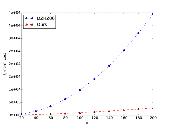
Figure 1: The $x$-axis is $n$ where $A\in\mathbb{R}^{n\times n}$, and the $y$-axis is $\|A^{\prime}-A\|_{1}$ where $\operatorname{rank}(A^{\prime})=k$. This figure shows the performance of both our algorithm and [DZHZ06] on input matrix $A$ defined as Equation (43).

The goal is to find a rank $k=1$ approximation for matrix $A$. For any $\epsilon\in[0,0.5)$, we define $A\in\mathbb{R}^{n\times n}$ as

$$A=\begin{bmatrix}n^{1.5+\epsilon}&0\\ 0&0\end{bmatrix}+\begin{bmatrix}0&0\\ 0&B\end{bmatrix},$$ (43)

where $B\in\mathbb{R}^{(n-1)\times(n-1)}$ is all $1$s matrix. It is immediate that the optimal cost is at most $n^{1.5+\epsilon}$. However, using the algorithm in [DZHZ06], the cost is at least $\Omega(n^{2})$. Thus, we can conclude, using algorithm [DZHZ06] to solve $\ell_{1}$ low rank approximation problem on $A$ cannot achieve an approximation ratio better than $n^{0.5-\epsilon}$.

L.3 Counterexample for [BDB13]

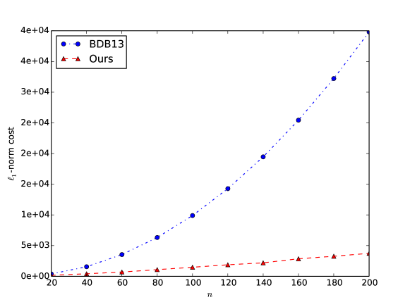
Figure 2: The $x$-axis is $n$ where $A\in\mathbb{R}^{n\times n}$, and the $y$-axis is $\|A^{\prime}-A\|_{1}$ where $\operatorname{rank}(A^{\prime})=k$. This figure shows the performance of both our algorithm and [BDB13] on input matrix $A$ defined as Equation (44).

The goal is to find a rank $k=1$ approximation for matrix $A$. The input matrix $A\in\mathbb{R}^{d\times d}$ for algorithm [BDB13] is defined to be,

$$A=\begin{bmatrix}n^{1.5}&0\\ 0&0\end{bmatrix}+\begin{bmatrix}0&0\\ 0&B\end{bmatrix},$$ (44)

where $B\in\mathbb{R}^{(n-1)\times(n-1)}$ is an all $1$s matrix. It is immediate that the optimal cost is at most $n^{1.5}$. Now, let us look at the procedure of [BDB13]. Basically, the algorithm described in [BDB13] is that they first find a rank $n-1$ approximation via a best $\ell_{1}$-fit hyperplane algorithm, then they rotate it based on the right singular vectors of the rank $n-1$ approximation matrix, and next they recursively do the same thing for the rotated matrix which has only $n-1$ columns.

When running their algorithm on $A$, they will fit an arbitrary column except the first column of $A$. Without loss of generality, it just fits the last column of $A$. After the rotation, the matrix will be an $n\times(n-1)$ matrix:

$$\begin{bmatrix}n^{1.5}&0&0&\cdots&0\\ 0&\sqrt{n-2}&0&\cdots&0\\ 0&\sqrt{n-2}&0&\cdots&0\\ \cdots&\cdots&\cdots&\cdots&\cdots\\ 0&\sqrt{n-2}&0&\cdots&0\end{bmatrix}.$$

Then, after the $t^{\text{th}}$ iteration for $t<(n-1)$, they will get an $n\times(n-t)$ matrix:

$$\begin{bmatrix}n^{1.5}&0&0&\cdots&0\\ 0&\sqrt{n-2}&0&\cdots&0\\ 0&\sqrt{n-2}&0&\cdots&0\\ \cdots&\cdots&\cdots&\cdots&\cdots\\ 0&\sqrt{n-2}&0&\cdots&0\end{bmatrix}.$$

This means that their algorithm will run on an $n\times 2$ matrix:

$$\begin{bmatrix}n^{1.5}&0\\ 0&\sqrt{n-2}\\ 0&\sqrt{n-2}\\ \cdots&\cdots\\ 0&\sqrt{n-2}\end{bmatrix},$$

in the last iteration. Notice that $n\times\sqrt{n-2}<n^{1.5}$. This means that their algorithm will fit the first column which implies that their algorithm will output a rank-$1$ approximation to $A$ by just fitting the first column of $A$. But the cost of this rank-$1$ solution is $(n-1)^{2}$. Since the optimal cost is at most $n^{1.5}$, their algorithm cannot achieve an approximation ratio better than $n^{0.5}$.

L.4 Counterexample for [Kwa08]

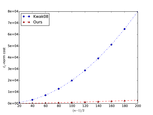
Figure 3: The $x$-axis is $n$ where $A\in\mathbb{R}^{n\times n}$, and the $y$-axis is $\|A^{\prime}-A\|_{1}$ where $\operatorname{rank}(A^{\prime})=k$. This figure shows the performance of both our algorithm and [Kwa08] on input matrix $A$ defined as Equation (45). Algorithm [Kwa08] has two ways of initialization, which have similar performance on matrix $A$.

We show that the algorithm [Kwa08] cannot achieve an approximation ratio better than $\Theta(n)$ on the matrix $A\in\mathbb{R}^{(2n+1)\times(2n+1)}$ defined as,

$$A=\begin{bmatrix}n^{1.5}&0&0\\ 0&B&0\\ 0&0&B\end{bmatrix},$$ (45)

where $B$ is an $n\times n$ matrix that contains all $1$s. We consider the rank-2 approximation problem for this input matrix $A$. The optimal cost is at most $n^{1.5}$.

We run their algorithm. Let $x_{0}$ denote the initial random unit vector. Consider the sign vector $s\in\{\pm 1\}^{2n+1}$ where each entry is the sign of the inner product between $x_{0}$ and each column of $A$. There are only three possibilities,

$$s=\begin{cases}(1,\{1\}^{n},\{1\}^{n})\\ (1,\{1\}^{n},\{-1\}^{n})\\ (1,\{-1\}^{n},\{1\}^{n})\\ \end{cases}.$$

Case i@, $s=(1,\{1\}^{n},\{1\}^{n})$. Define $\widehat{u}=\sum_{i=1}^{2n+1}s_{i}\cdot A_{i}=(n^{1.5},n,\cdots,n)$. Let $u=\widehat{u}/\|u\|_{2}=\widehat{u}/(\sqrt{3}n^{1.5})=(1/\sqrt{3},1/\sqrt{3n},\cdots,1/\sqrt{3n})$. Define matrix $D$ to be $A-uu^{\top}A$. Then, we can compute $D$,

$$D= \leavevmode\nobreak\ A-uu^{\top}A$$

$$= \leavevmode\nobreak\ A-\begin{bmatrix}1/3&\frac{1}{3\sqrt{n}}{\bf 1}^{\top}&\frac{1}{3\sqrt{n}}{\bf 1}^{\top}\\ \frac{1}{3\sqrt{n}}{\bf 1}&\frac{1}{3n}B&\frac{1}{3n}B\\ \frac{1}{3\sqrt{n}}{\bf 1}&\frac{1}{3n}B&\frac{1}{3n}B\end{bmatrix}A$$

$$= \begin{bmatrix}n^{1.5}&0&0\\ 0&B&0\\ 0&0&B\end{bmatrix}-\begin{bmatrix}\frac{n^{1.5}}{3}&\frac{\sqrt{n}}{3}{\bf 1}^{\top}&\frac{\sqrt{n}}{3}{\bf 1}^{\top}\\ \frac{n}{3}{\bf 1}&\frac{1}{3}B&\frac{1}{3}B\\ \frac{n}{3}{\bf 1}&\frac{1}{3}B&\frac{1}{3}B\\ \end{bmatrix}$$

$$= \begin{bmatrix}2n^{1.5}/3&-\frac{\sqrt{n}}{3}{\bf 1}^{\top}&-\frac{\sqrt{n}}{3}{\bf 1}^{\top}\\ -\frac{n}{3}{\bf 1}&\frac{2}{3}B&-\frac{1}{3}B\\ -\frac{n}{3}{\bf 1}&-\frac{1}{3}B&\frac{2}{3}B\\ \end{bmatrix}.$$

Now we need to take the linear combination of columns $D=A-uu^{\top}A$. Let $w$ denote another sign vector $\{-1,+1\}^{2n+1}$. Then let $v$ denote the basis vector, $v=\sum_{i=1}^{2n+1}D_{i}$. There are three possibilities, Case I(a), if $w=(1,\{1\}^{n},\{1\}^{n})$, then $v$ is the all $0$ vector. Using vector $v$ to interpolate each column of $D$, the cost we obtain is at least $2n^{2}$. Case I(b), if $w=(1,\{1\}^{n},\{-1\}^{n})$, then $v=(2n^{1.5}/3,\{2/3\}^{n},\{-4/3\}^{n})$. We also obtain at least $2n^{2}$ cost if we use that $v$ to interpolate each column of $D$. Case I(c), if $w=(1,\{-1\}^{n},\{-1\}^{n})$, then $v=(0,\{-2/3\}^{n},\{-2/3\}^{n})$. The cost is also at least $2n^{2}$.

Case ii@, $s=(1,\{1\}^{n},\{-1\}^{n})$. Define ${\bf 1}$ to be a length $n$ all $1$s column vector. Define $\widehat{u}=\sum_{i=1}^{2n+1}s_{i}\cdot A_{i}=(n^{1.5},\{n\}^{n},\{-n\}^{n})$. Let $u=\widehat{u}/\|u\|_{2}=\widehat{u}/(\sqrt{3}n^{1.5})=(1/\sqrt{3},\{1/\sqrt{3n}\}^{n},\{-1/\sqrt{3n}\}^{n})$. Define $(2n+1)\times(2n+1)$ matrix $D$ to be $A-uu^{\top}A$. Then, we can compute $D$,

$$D= \leavevmode\nobreak\ A-uu^{\top}A$$

$$= \leavevmode\nobreak\ A-\begin{bmatrix}1/3&\frac{1}{3\sqrt{n}}{\bf 1}^{\top}&-\frac{1}{3\sqrt{n}}{\bf 1}^{\top}\\ \frac{1}{3\sqrt{n}}{\bf 1}&\frac{1}{3n}B&-\frac{1}{3n}B\\ -\frac{1}{3\sqrt{n}}{\bf 1}&-\frac{1}{3n}B&\frac{1}{3n}B\\ \end{bmatrix}A$$

$$= \begin{bmatrix}n^{1.5}&0&0\\ 0&B&0\\ 0&0&B\end{bmatrix}-\begin{bmatrix}n^{1.5}/3&\frac{\sqrt{n}}{3}{\bf 1}^{\top}&-\frac{\sqrt{n}}{3}{\bf 1}^{\top}\\ \frac{n}{3}{\bf 1}&\frac{1}{3}B&-\frac{1}{3}B\\ -\frac{n}{3}{\bf 1}&-\frac{1}{3}B&\frac{1}{3}B\\ \end{bmatrix}$$

$$= \begin{bmatrix}2n^{1.5}/3&-\frac{\sqrt{n}}{3}{\bf 1}^{\top}&\frac{\sqrt{n}}{3}{\bf 1}^{\top}\\ -\frac{n}{3}{\bf 1}&\frac{2}{3}B&\frac{1}{3}B\\ \frac{n}{3}{\bf 1}&\frac{1}{3}B&\frac{2}{3}B\\ \end{bmatrix}.$$

Similarly to the previous case, we can also discuss three cases.

Case iii@, $s=(1,\{1\}^{n},\{-1\}^{n})$. Define ${\bf 1}$ to be a length $n$ all $1$s column vector. Define $\widehat{u}=\sum_{i=1}^{2n+1}s_{i}\cdot A_{i}=(n^{1.5},\{-n\}^{n},\{-n\}^{n})$. Let $u=\widehat{u}/\|u\|_{2}=\widehat{u}/(\sqrt{3}n^{1.5})=(1/\sqrt{3},\{-1/\sqrt{3n}\}^{n},\{-1/\sqrt{3n}\}^{n})$. Define matrix $D$ to be $A-uu^{\top}A$. Then, we can compute $D$,

$$D= \leavevmode\nobreak\ A-uu^{\top}A$$

$$= \leavevmode\nobreak\ A-\begin{bmatrix}1/3&-\frac{1}{3\sqrt{n}}){\bf 1}^{\top}&-\frac{1}{3\sqrt{n}}{\bf 1}^{\top}\\ -\frac{1}{3\sqrt{n}}{\bf 1}&\frac{1}{3n}B&\frac{1}{3n}B\\ -\frac{1}{3\sqrt{n}}{\bf 1}&\frac{1}{3n}B&\frac{1}{3n}B\\ \end{bmatrix}A$$

$$= \begin{bmatrix}n^{1.5}&0&0\\ 0&B&0\\ 0&0&B\end{bmatrix}-\begin{bmatrix}n^{1.5}/3&-\frac{\sqrt{n}}{3}{\bf 1}^{\top}&-\frac{\sqrt{n}}{3}{\bf 1}^{\top}\\ -\frac{n}{3}{\bf 1}&\frac{1}{3}B&\frac{1}{3}B\\ -\frac{n}{3}{\bf 1}&\frac{1}{3}B&\frac{1}{3}B\\ \end{bmatrix}$$

$$= \begin{bmatrix}2n^{1.5}/3&\frac{\sqrt{n}}{3}{\bf 1}^{\top}&\frac{\sqrt{n}}{3}{\bf 1}^{\top}\\ \frac{n}{3}{\bf 1}&\frac{2}{3}B&\frac{1}{3}B\\ \frac{n}{3}{\bf 1}&\frac{1}{3}B&\frac{2}{3}B\\ \end{bmatrix}.$$

Similarly to the previous case, we can also discuss three cases.

L.5 Counterexample for [KK05]

We show that there exist matrices such that the algorithm of [KK05] cannot achieve an approximation ratio better than $\Theta(n)$. Their algorithm has two different ways of initialization. We provide counterexamples for each of the initialization separately.

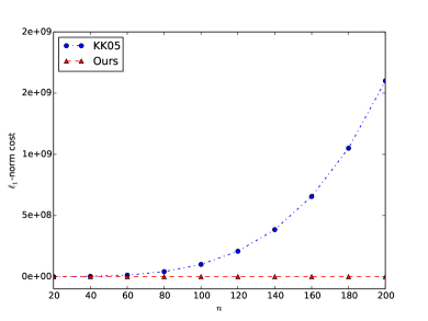
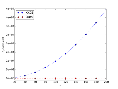
Figure 4: The $x$-axis is $n$ where $A\in\mathbb{R}^{n\times n}$, and the $y$-axis is $\|A^{\prime}-A\|_{1}$ where $\operatorname{rank}(A^{\prime})=k$. Algorithm [KK05] has two ways of initialization. The left figure shows the performance of both our algorithm and [KK05] with random vector initialization on input matrix $A$ defined as Equation (46). The right figure shows the performance of both our algorithm and [KK05] with top singular vector initialization on input matrix $A$ defined as Equation (48).

Random vector initialization

We provide a counterexample matrix $A\in\mathbb{R}^{n\times n}$ defined as,

$$A=\begin{bmatrix}n^{c}&0&\cdots&0\\ 0&0&\cdots&0\\ \cdots&\cdots&\cdots&\cdots\\ 0&0&\cdots&0\end{bmatrix}+I,$$ (46)

where $c\geq 2$. Consider the rank-1 approximation problem for this matrix $A$. The optimal cost is at most $n-1$.

Run their algorithm. The starting vectors are $u(0)\sim N(0,I)$ and $v(0)\sim N(0,1)$. We define two properties for a given vector $y\in\mathbb{R}^{n}$. Property i@ is for all $i\in[n]$, $|y_{i}|\leq n/8$, and Property ii@ is there exist half of the $i$ such that $|y_{i}|\geq 1/2$. We can show that with probability $1-2^{-\Omega(n)}$, both $u(0)$ and $v(0)$ satisfy Property i@ and ii@. After $1$ iteration, we can show that $u(1)_{1}=v(1)_{1}=0$

Now let us use column vector $u(0)\in\mathbb{R}^{n}$ to interpolate the first column of matrix $A$. We simplify $u(0)$ to be $u$. Let $u_{i}$ denote the $i$-th coordinate of vector $u$, $\forall i\in[n]$. Let $A_{1}$ denote the first column of matrix $A$. We define $\alpha=v(1)_{1}=\arg\min_{\alpha}\|\alpha u(0)-A_{1}\|_{1}$. For any scalar $\alpha$, the cost we pay on the first column of matrix $A$ is,

$$\leavevmode\nobreak\ |\alpha\cdot u_{1}-n^{c}|+\sum_{i=2}^{n}|\alpha u_{i}|\geq\leavevmode\nobreak\ |\alpha\cdot u_{1}-n^{c}|+\frac{n}{2}|\alpha\cdot\frac{1}{2}|\geq\leavevmode\nobreak\ |\alpha\cdot u_{1}-n^{c}|+\frac{n}{4}|\alpha|.$$ (47)

Notice that $c\geq 2$. Then $|\alpha\cdot u_{1}-n^{c}|+\frac{n}{4}|\alpha|\geq|\alpha\cdot\frac{n}{8}-n^{c}|+\frac{n}{4}|\alpha|$. If $\alpha\leq 0$, then the cost is minimized when $\alpha=0$. If $\alpha\in[0,8n^{c-1}]$, the cost is minimized when $\alpha=0$. If $\alpha\geq 8n^{c-1}$, the cost is minimized when $\alpha=8n^{c-1}$. Putting it all together, to achieve the minimum cost, there is only one choice for $\alpha$, which is $\alpha=0$. The optimal cost is at least $n^{c}$.

Then after $T$ iterations(for any $T\geq 1$), $u(T)_{1}=v(T)_{1}=0$. Thus, we always pay at least $n^{c}$ cost on the first entry.

Therefore, their algorithm cannot achieve any approximation ratio better than $n^{c-1}$. Because $c\geq 2$, we complete the proof.

Top singular vector initialization

The counterexample input matrix $A\in\mathbb{R}^{n\times n}$ is defined as,

$$A=\begin{bmatrix}n&0\\ 0&B\\ \end{bmatrix},$$ (48)

where matrix $B\in\mathbb{R}^{(n-1)\times(n-1)}$ contains all $1$s. Consider the rank-1 approximation problem for this matrix $A$. The optimal cost is at most $n$. Run their algorithm. The starting vectors $u(0)$ and $v(0)$ will be set to $(1,0,\cdots,0)\in\mathbb{R}^{n}$. After $T$ iterations(for any $T>0$), the support of $u(T)$(resp. $v(T)$) is the same as $u(0)$(resp. $v(T)$). Thus, the cost is at least $\|B\|_{1}=(n-1)^{2}$. Therefore, we can conclude that their algorithm cannot achieve any approximation ratio better than $(n-1)^{2}/n=\Theta(n)$.

L.6 Counterexample for all

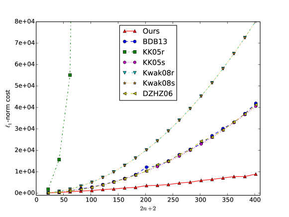
(a)

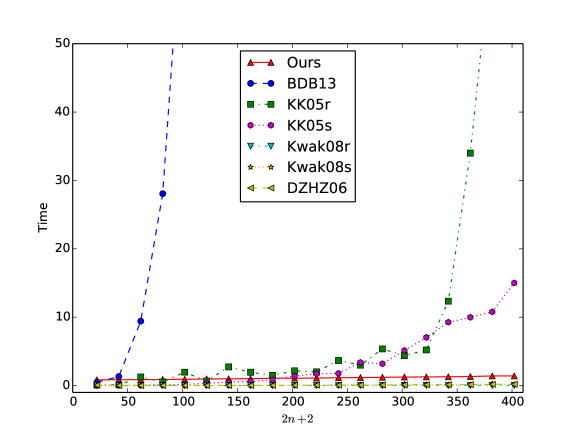
(b)

Figure 5: Let $A$ be $(2n+2)\times(2n+2)$ input matirx. (a) shows the performance of all the algorithms when the matrix dimension is growing. The $x$-axis is $n$, and the $y$-axis is $\|A^{\prime}-A\|_{1}$ where $A^{\prime}$ is the rank-$3$ solution output by all the heuristic algorithms and also ours. The $\ell_{1}$ residual cost of all the other algorithms is growing much faster than ours, which is consistent with our theoretical results. (b) shows the running time (in seconds) of all the algorithms when the matrix dimension $n$ is growing. The $x$-axis is $n$ and the $y$-axis is time (seconds). The running time of some of the algorithms is longer than $3$ seconds. For most of the algorithms (including ours), the running time is always less than $3$ seconds.

For any $\epsilon\in(0,0.5)$ and $\gamma>0$, we construct the input matrix $A\in\mathbb{R}^{(2n+2)\times(2n+2)}$ as follows

$$A=\begin{bmatrix}n^{2+\gamma}&0&0&0\\ 0&n^{1.5+\epsilon}&0&0\\ 0&0&B&0\\ 0&0&0&B\end{bmatrix},$$

where $B$ is $n\times n$ all $1$s matrix. We want to find a rank $k=3$ solution for $A$. Then any of those four heuristic algorithms [KK05, DZHZ06, Kwa08, BDB13] is not able to achieve better than $n^{\min(\gamma,0.5-\epsilon)}$ approximation ratio. We present our main experimental results in Figure 5. Both [KK05] and [Kwa08] have two different ways of initialization. In Figure 5 we use KK05r(resp. Kwak08r) to denote the way that uses random vector as initialization, and use KK05s(resp. Kwak08s) to denote the way that uses top singular vector as initialization. Figure 5(a) shows the performance of all the algorithms and Figure 5(b) presents the running time. The $\ell_{1}$ residual cost of all the other algorithm is growing much faster than our algorithm. Most of the algorithms (including ours) are pretty efficient, i.e., the running time is always below $3$ seconds. The running time of [BDB13, KK05] is increasing very fast when the matrix dimension $n$ is growing.

In Figure 5(a), the cost of KK05r at $\{82,\cdots,142\}$ is in $[10^{5},10^{6}]$, at $\{162,\cdots,302\}$ is in $[10^{6},10^{7}]$, and at $\{322,\cdots,402\}$ is in $[10^{7},10^{8}]$. In Figure 5(b), the time of KK05r at $\{382,482\}$ is $64$s and $160$s. The running time of BDB13 at $\{82,\cdots,222\}$ is between $1$ minute and $1$ hour. The running time of BDB13 at $\{242,\cdots,322\}$ is between $1$ hour and $20$ hours. The running time of BDB13 at $\{342,\cdots,402\}$ is more than $20$ hours.

L.7 Discussion for Robust PCA [CLMW11]

A popular method is robust PCA [CLMW11], which given a matrix $A$, tries to find a matrix $L$ for which $\lambda\|A-L\|_{1}+\|L\|_{*}$ is minimized, where $\lambda>0$ is a tuning parameter and $\|L\|_{*}$ is the nuclear norm of $L$. This is a convex program, but it need not return a low rank matrix $L$ with relative error. As a simple example, suppose $\lambda=1$, and the $n\times n$ matrix $A$ is a block-diagonal matrix of rank $k$ and $n=\frac{k}{2}(b+1)$. Further, the first $k/2$ blocks are $b\times b$ matrices of all $1$s, while the next $k/2$ blocks are just a single value $b$ on the diagonal.

Then the solution to the above problem may return $L$ to be the first $k/2$ blocks of $A$. The total cost of $\lambda\|A-L\|_{1}+\|L\|_{*}$is $(k/2)b+(k/2)b=kb$.

Also, the solution to the above problem may return $L$ to be $A$, which has cost $0+\|A\|_{*}=kb$. Because this solution has the same cost, it means that their algorithm might output a rank-$k$ solution, and also might output a rank-$k/2$ solution.

Therefore, the relative error of the output matrix may be arbitrarily bad for $\ell_{1}$-low rank approximation.

We also consider the following example. Suppose $\lambda=1/\sqrt{n}$, and let $n\times n$ matrix $A$ denote the Hadamard matrix $H_{n}$. Recall that the Hadamard matrix $H_{p}$ of size $p\times p$ is defined recursively : $\begin{bmatrix}H_{p/2}&H_{p/2}\\ H_{p/2}&-H_{p/2}\end{bmatrix}$ with $H_{2}=\begin{bmatrix}+1&+1\\ +1&-1\end{bmatrix}$. Notice that every singular values of $A$ is $\sqrt{n}$. We consider the objective function $\lambda\|A-L\|_{1}+\|L\|_{*}$.

Then the solution to the above problem may return $L$ to be the first $n/2$ rows of $A$. The total cost of $\lambda\|A-L\|_{1}+\|L\|_{*}$ is $(1/\sqrt{n})n^{2}/2+(n/2)\sqrt{n}=n^{1.5}$. Also, the solution to the above problem may return $L$ to be $A$, which has cost $0+\|A\|_{*}=n\sqrt{n}=n^{1.5}$. For any $i$, if the solution takes $i$ rows of $A$, the cost is $(1/\sqrt{n})(n-i)n+i\sqrt{n}=n^{1.5}$. Because this solution has the same cost, it means that their algorithm might output a rank-$n$ solution, and also might output a rank-$n/2$ solution. Therefore, the relative error of the output matrix may be arbitrarily bad for $\ell_{1}$-low rank approximation.

Appendix M Acknowledgments

The authors would like to thank Alexandr Andoni, Saugata Basu, Cho-Jui Hsieh, Daniel Hsu, Chi Jin, Fu Li, Ankur Moitra, Cameron Musco, Richard Peng, Eric Price, Govind Ramnarayan, James Renegar, and Clifford Stein for useful discussions. The authors also thank Jiyan Yang, Yinlam Chow, Christopher Ré, and Michael Mahoney for sharing the code.

References

- [AB09] Sanjeev Arora and Boaz Barak. Computational complexity: a modern approach. Cambridge University Press, 2009.
- [ABIW09] Alexandr Andoni, Khanh Do Ba, Piotr Indyk, and David P Woodruff. Efficient sketches for earth-mover distance, with applications. In 50th Annual IEEE Symposium on Foundations of Computer Science, pages 324–330, 2009.
- [AGKM12] Sanjeev Arora, Rong Ge, Ravindran Kannan, and Ankur Moitra. Computing a nonnegative matrix factorization - provably. In Proceedings of the 44th Symposium on Theory of Computing Conference, STOC 2012, New York, NY, USA, May 19 - 22, 2012, pages 145–162, 2012.
- [AIK08] Alexandr Andoni, Piotr Indyk, and Robert Krauthgamer. Earth mover distance over high-dimensional spaces. In Proceedings of the nineteenth annual ACM-SIAM symposium on Discrete algorithms, pages 343–352. Society for Industrial and Applied Mathematics, 2008.
- [Bas14] Saugata Basu. Algorithms in real algebraic geometry: a survey. arXiv preprint arXiv:1409.1534, 2014.
- [BCL05] Zheng-Jian Bai, Raymond H Chan, and Franklin T Luk. Principal component analysis for distributed data sets with updating. In Advanced Parallel Processing Technologies, pages 471–483. Springer, 2005.
- [BD13] J. Paul Brooks and José H. Dulá. The -norm best-fit hyperplane problem. Appl. Math. Lett., 26(1):51–55, 2013.
- [BDB13] J. Paul Brooks, José H. Dulá, and Edward L Boone. A pure -norm principal component analysis. Computational statistics & data analysis, 61:83–98, 2013.
- [BDL16] Amitabh Basu, Michael Dinitz, and Xin Li. Computing approximate PSD factorizations. CoRR, abs/1602.07351, 2016.
- [BDM11] Christos Boutsidis, Petros Drineas, and Malik Magdon-Ismail. Near optimal column-based matrix reconstruction. In IEEE 52nd Annual Symposium on Foundations of Computer Science, FOCS 2011, Palm Springs, CA, USA, October 22-25, 2011, pages 305–314, 2011.
- [BDN15] Jean Bourgain, Sjoerd Dirksen, and Jelani Nelson. Toward a unified theory of sparse dimensionality reduction in euclidean space. In Proceedings of the Forty-Seventh Annual ACM on Symposium on Theory of Computing, STOC 2015, Portland, OR, USA, June 14-17, 2015, pages 499–508, 2015.
- [BGS98] Mihir Bellare, Oded Goldreich, and Madhu Sudan. Free bits, pcps, and nonapproximability—towards tight results. SIAM Journal on Computing, 27(3):804–915, 1998.
- [BIRW16] Arturs Backurs, Piotr Indyk, Ilya Razenshteyn, and David P Woodruff. Nearly-optimal bounds for sparse recovery in generic norms, with applications to k-median sketching. In Proceedings of the Twenty-Seventh Annual ACM-SIAM Symposium on Discrete Algorithms, pages 318–337. SIAM, 2016.
- [BJ12] J. Paul Brooks and Sapan Jot. Pcal1: An implementation in r of three methods for -norm principal component analysis. Optimization Online preprint, 2012.
- [BKLW14] Maria-Florina Balcan, Vandana Kanchanapally, Yingyu Liang, and David Woodruff. Improved distributed principal component analysis. NIPS, 2014.
- [BLS+16] Maria-Florina Balcan, Yingyu Liang, Le Song, David Woodruff, and Bo Xie. Distributed kernel principal component analysis. KDD, 2016.
- [BMD09] Christos Boutsidis, Michael W Mahoney, and Petros Drineas. An improved approximation algorithm for the column subset selection problem. In Proceedings of the twentieth Annual ACM-SIAM Symposium on Discrete Algorithms, pages 968–977. Society for Industrial and Applied Mathematics, 2009.
- [BPR96] Saugata Basu, Richard Pollack, and Marie-Françoise Roy. On the combinatorial and algebraic complexity of quantifier elimination. J. ACM, 43(6):1002–1045, 1996.
- [BPR05] Saugata Basu, Richard Pollack, and Marie-Francoise Roy. Algorithms in real algebraic geometry, volume 20033. Springer, 2005.
- [BRB08] Yann-Ael Le Borgne, Sylvain Raybaud, and Gianluca Bontempi. Distributed principal component analysis for wireless sensor networks. Sensors, 2008.
- [BW14] Christos Boutsidis and David P Woodruff. Optimal cur matrix decompositions. In Proceedings of the 46th Annual ACM Symposium on Theory of Computing, pages 353–362. ACM, 2014.
- [BWZ16] Christos Boutsidis, David P Woodruff, and Peilin Zhong. Optimal principal component analysis in distributed and streaming models. In Proceedings of the 48th Annual ACM SIGACT Symposium on Theory of Computing, pages 236–249. ACM, 2016.
- [CDMI+13] Kenneth L Clarkson, Petros Drineas, Malik Magdon-Ismail, Michael W Mahoney, Xiangrui Meng, and David P Woodruff. The fast cauchy transform and faster robust linear regression. In Proceedings of the Twenty-Fourth Annual ACM-SIAM Symposium on Discrete Algorithms, pages 466–477. Society for Industrial and Applied Mathematics, 2013.
- [CGK+16] Flavio Chierichetti, Sreenivas Gollapudi, Ravi Kumar, Silvio Lattanzi, and Rina Panigrahy. On robust low-rank approximation. ArXiv e-prints, 2016.
- [CHD16] Kai-Yang Chiang, Cho-Jui Hsieh, and Inderjit S Dhillon. Robust principal component analysis with side information. In Proceedings of The 33rd International Conference on Machine Learning, pages 2291–2299, 2016.
- [CK11] Imre Csiszar and János Körner. Information theory: coding theorems for discrete memoryless systems. Cambridge University Press, 2011.
- [Cla05] Kenneth L Clarkson. Subgradient and sampling algorithms for regression. In Proceedings of the sixteenth annual ACM-SIAM symposium on Discrete algorithms, pages 257–266, 2005.
- [CLM+15] Michael B Cohen, Yin Tat Lee, Cameron Musco, Christopher Musco, Richard Peng, and Aaron Sidford. Uniform sampling for matrix approximation. In Proceedings of the 2015 Conference on Innovations in Theoretical Computer Science, pages 181–190. ACM, 2015.
- [CLMW11] Emmanuel J Candès, Xiaodong Li, Yi Ma, and John Wright. Robust principal component analysis? Journal of the ACM (JACM), 58(3):11, 2011.
- [Coh16] Michael B. Cohen. Nearly tight oblivious subspace embeddings by trace inequalities. In Proceedings of the Twenty-Seventh Annual ACM-SIAM Symposium on Discrete Algorithms, SODA 2016, Arlington, VA, USA, January 10-12, 2016, pages 278–287, 2016.
- [CP15] Michael B. Cohen and Richard Peng. row sampling by lewis weights. In Proceedings of the Forty-Seventh Annual ACM on Symposium on Theory of Computing, STOC ’15, pages 183–192, New York, NY, USA, 2015. ACM.
- [CW87] Don Coppersmith and Shmuel Winograd. Matrix multiplication via arithmetic progressions. In Proceedings of the nineteenth annual ACM symposium on Theory of computing, pages 1–6. ACM, 1987.
- [CW09] Kenneth L. Clarkson and David P. Woodruff. Numerical linear algebra in the streaming model. In Proceedings of the 41st Annual ACM Symposium on Theory of Computing, STOC 2009, Bethesda, MD, USA, May 31 - June 2, 2009, pages 205–214, 2009.
- [CW13] Kenneth L. Clarkson and David P. Woodruff. Low rank approximation and regression in input sparsity time. In Symposium on Theory of Computing Conference, STOC’13, Palo Alto, CA, USA, June 1-4, 2013, pages 81–90, 2013.
- [CW15a] Kenneth L Clarkson and David P Woodruff. Input sparsity and hardness for robust subspace approximation. In Foundations of Computer Science (FOCS), 2015 IEEE 56th Annual Symposium on, pages 310–329. IEEE, 2015.
- [CW15b] Kenneth L Clarkson and David P Woodruff. Sketching for m-estimators: A unified approach to robust regression. In Proceedings of the Twenty-Sixth Annual ACM-SIAM Symposium on Discrete Algorithms, pages 921–939. SIAM, 2015.
- [DDH+09] Anirban Dasgupta, Petros Drineas, Boulos Harb, Ravi Kumar, and Michael W Mahoney. Sampling algorithms and coresets for regression. SIAM Journal on Computing, 38(5):2060–2078, 2009.
- [DMM06a] Petros Drineas, Michael W. Mahoney, and S. Muthukrishnan. Subspace sampling and relative-error matrix approximation: Column-based methods. In Approximation, Randomization, and Combinatorial Optimization. Algorithms and Techniques, 9th International Workshop on Approximation Algorithms for Combinatorial Optimization Problems, APPROX 2006 and 10th International Workshop on Randomization and Computation, RANDOM 2006, Barcelona, Spain, August 28-30 2006, Proceedings, pages 316–326, 2006.
- [DMM06b] Petros Drineas, Michael W. Mahoney, and S. Muthukrishnan. Subspace sampling and relative-error matrix approximation: Column-row-based methods. In Algorithms - ESA 2006, 14th Annual European Symposium, Zurich, Switzerland, September 11-13, 2006, Proceedings, pages 304–314, 2006.
- [DMM08] Petros Drineas, Michael W. Mahoney, and S. Muthukrishnan. Relative-error CUR matrix decompositions. SIAM J. Matrix Analysis Applications, 30(2):844–881, 2008.
- [DR10] Amit Deshpande and Luis Rademacher. Efficient volume sampling for row/column subset selection. In Foundations of Computer Science (FOCS), 2010 51st Annual IEEE Symposium on, pages 329–338. IEEE, 2010.
- [DV07] Amit Deshpande and Kasturi R. Varadarajan. Sampling-based dimension reduction for subspace approximation. In Proceedings of the 39th Annual ACM Symposium on Theory of Computing, San Diego, California, USA, June 11-13, 2007, pages 641–650, 2007.
- [DZHZ06] Chris Ding, Ding Zhou, Xiaofeng He, and Hongyuan Zha. R1-pca: rotational invariant -norm principal component analysis for robust subspace factorization. In Proceedings of the 23rd international conference on Machine learning, pages 281–288. ACM, 2006.
- [Exc13] Stack Exchange. Low-rank matrix approximation in terms of entry-wise norm, 2013.
- [FEGK13] Ahmed K Farahat, Ahmed Elgohary, Ali Ghodsi, and Mohamed S Kamel. Distributed column subset selection on mapreduce. In Data Mining (ICDM), 2013 IEEE 13th International Conference on, pages 171–180. IEEE, 2013.
- [FL11] Dan Feldman and Michael Langberg. A unified framework for approximating and clustering data. In Proceedings of the 43rd ACM Symposium on Theory of Computing, STOC 2011, San Jose, CA, USA, 6-8 June 2011, pages 569–578, 2011.
- [FLP15] Dimitris Fotakis, Michael Lampis, and Vangelis Th Paschos. Sub-exponential approximation schemes for csps: From dense to almost sparse. arXiv preprint arXiv:1507.04391, 2015.
- [FMSW10] Dan Feldman, Morteza Monemizadeh, Christian Sohler, and David P. Woodruff. Coresets and sketches for high dimensional subspace approximation problems. In Proceedings of the Twenty-First Annual ACM-SIAM Symposium on Discrete Algorithms, SODA 2010, Austin, Texas, USA, January 17-19, 2010, pages 630–649, 2010.
- [FT07] Shmuel Friedland and Anatoli Torokhti. Generalized rank-constrained matrix approximations. SIAM Journal on Matrix Analysis and Applications, 29(2):656–659, 2007.
- [Gao08] Junbin Gao. Robust principal component analysis and its bayesian variational inference. Neural computation, 20(2):555–572, 2008.
- [GP13] M. Ghashami and J.M. Phillips. Relative errors for deterministic low-rank matrix approximations. In SODA, 2013.
- [GV15] Nicolas Gillis and Stephen A Vavasis. On the complexity of robust pca and -norm low-rank matrix approximation. arXiv preprint arXiv:1509.09236, 2015.
- [GW95] Michel X Goemans and David P Williamson. Improved approximation algorithms for maximum cut and satisfiability problems using semidefinite programming. Journal of the ACM (JACM), 42(6):1115–1145, 1995.
- [Hås01] Johan Håstad. Some optimal inapproximability results. Journal of the ACM (JACM), 48(4):798–859, 2001.
- [Ind06] Piotr Indyk. Stable distributions, pseudorandom generators, embeddings, and data stream computation. Journal of the ACM (JACM), 53(3):307–323, 2006.
- [IP11] Piotr Indyk and Eric Price. K-median clustering, model-based compressive sensing, and sparse recovery for earth mover distance. In Proceedings of the forty-third annual ACM symposium on Theory of computing, pages 627–636. ACM, 2011.
- [IPZ98] Russell Impagliazzo, Ramamohan Paturi, and Francis Zane. Which problems have strongly exponential complexity? In Foundations of Computer Science, 1998. Proceedings. 39th Annual Symposium on, pages 653–662. IEEE, 1998.
- [IT03] Piotr Indyk and Nitin Thaper. Fast image retrieval via embeddings. In Workshop on Statistical and Computational Theories of Vision (at ICCV), 2003.
- [KAC+08] Fredrik Kahl, Sameer Agarwal, Manmohan Krishna Chandraker, David Kriegman, and Serge Belongie. Practical global optimization for multiview geometry. International Journal of Computer Vision, 79(3):271–284, 2008.
- [KK03] Qifa Ke and Takeo Kanade. Robust subspace computation using norm. Technical Report CMU-CS-03-172, Carnegie Mellon University, Pittsburgh, PA., 2003.
- [KK05] Qifa Ke and Takeo Kanade. Robust norm factorization in the presence of outliers and missing data by alternative convex programming. In 2005 IEEE Computer Society Conference on Computer Vision and Pattern Recognition (CVPR’05), volume 1, pages 739–746. IEEE, 2005.
- [KKMO07] Subhash Khot, Guy Kindler, Elchanan Mossel, and Ryan O’Donnell. Optimal inapproximability results for max-cut and other 2-variable csps? SIAM Journal on Computing, 37(1):319–357, 2007.
- [KL11] J. Kelner and A. Levin. Spectral sparsification in the semi-streaming setting. In Symposium on Theoretical Aspects of Computer Science (STACS), 2011.
- [KLC+15] Eunwoo Kim, Minsik Lee, Chong-Ho Choi, Nojun Kwak, and Songhwai Oh. Efficient-norm-based low-rank matrix approximations for large-scale problems using alternating rectified gradient method. IEEE transactions on neural networks and learning systems, 26(2):237–251, 2015.
- [KLM+14] Michael Kapralov, Yin Tat Lee, Cameron Musco, Christopher Musco, and Aaron Sidford. Single pass spectral sparsification in dynamic streams. In Foundations of Computer Science (FOCS), 2014 IEEE 55th Annual Symposium on, pages 561–570. IEEE, 2014.
- [KNW10] Daniel M Kane, Jelani Nelson, and David P Woodruff. On the exact space complexity of sketching and streaming small norms. In Proceedings of the twenty-first annual ACM-SIAM symposium on Discrete Algorithms, pages 1161–1178. Society for Industrial and Applied Mathematics, 2010.
- [KV09] Ravi Kannan and Santosh Vempala. Spectral algorithms. Foundations and Trends in Theoretical Computer Science, 4(3-4):157–288, 2009.
- [KVW14] Ravindran Kannan, Santosh S Vempala, and David P Woodruff. Principal component analysis and higher correlations for distributed data. In Proceedings of The 27th Conference on Learning Theory, pages 1040–1057, 2014.
- [Kwa08] Nojun Kwak. Principal component analysis based on -norm maximization. IEEE transactions on pattern analysis and machine intelligence, 30(9):1672–1680, 2008.
- [Lib13] Edo Liberty. Simple and deterministic matrix sketching. In KDD, pages 581–588. ACM, 2013.
- [LMP13] Mu Li, Gary L. Miller, and Richard Peng. Iterative row sampling. In 54th Annual IEEE Symposium on Foundations of Computer Science, FOCS 2013, 26-29 October, 2013, Berkeley, CA, USA, pages 127–136, 2013.
- [LOG16] Wuchen Li, Stanley Osher, and Wilfrid Gangbo. Fast algorithm for earth mover’s distance based on optimal transport and type regularization i. arXiv preprint arXiv:1609.07092, 2016.
- [LPW09] David Asher Levin, Yuval Peres, and Elizabeth Lee Wilmer. Markov chains and mixing times. American Mathematical Soc., 2009.
- [MBZ10] Sergio V Macua, Pavle Belanovic, and Santiago Zazo. Consensus-based distributed principal component analysis in wireless sensor networks. In Signal Processing Advances in Wireless Communications (SPAWC), 2010 IEEE Eleventh International Workshop on, pages 1–5. IEEE, 2010.
- [McG06] Andrew McGregor. Open problems in data streams and related topics. In IITK Workshop on Algorithms For Data Streams, 2006.
- [MKCP16] P. P. Markopoulos, S. Kundu, S. Chamadia, and D. A. Pados. Efficient -Norm Principal-Component Analysis via Bit Flipping. ArXiv e-prints, 2016.
- [MKP13] Panos P. Markopoulos, George N. Karystinos, and Dimitrios A. Pados. Some options for -subspace signal processing. In ISWCS 2013, The Tenth International Symposium on Wireless Communication Systems, Ilmenau, TU Ilmenau, Germany, August 27-30, 2013, pages 1–5, 2013.
- [MKP14] Panos P. Markopoulos, George N. Karystinos, and Dimitrios A. Pados. Optimal algorithms for -subspace signal processing. IEEE Trans. Signal Processing, 62(19):5046–5058, 2014.
- [MM13] Xiangrui Meng and Michael W Mahoney. Low-distortion subspace embeddings in input-sparsity time and applications to robust linear regression. In Proceedings of the forty-fifth annual ACM symposium on Theory of computing, pages 91–100. ACM, 2013.
- [Moi13] Ankur Moitra. An almost optimal algorithm for computing nonnegative rank. In Proceedings of the Twenty-Fourth Annual ACM-SIAM Symposium on Discrete Algorithms, SODA 2013, New Orleans, Louisiana, USA, January 6-8, 2013, pages 1454–1464, 2013.
- [Mut05] S. Muthukrishnan. Data Streams: Algorithms and Applications. Foundations and Trends in Theoretical Computer Science, 1(2):117–236, 2005.
- [MXZZ13] Deyu Meng, Zongben Xu, Lei Zhang, and Ji Zhao. A cyclic weighted median method for low-rank matrix factorization with missing entries. In AAAI, volume 4, page 6, 2013.
- [NN13] Jelani Nelson and Huy L Nguyên. Osnap: Faster numerical linear algebra algorithms via sparser subspace embeddings. In Foundations of Computer Science (FOCS), 2013 IEEE 54th Annual Symposium on, pages 117–126. IEEE, 2013.
- [NN14] Jelani Nelson and Huy L Nguyên. Lower bounds for oblivious subspace embeddings. In International Colloquium on Automata, Languages, and Programming, pages 883–894. Springer, 2014.
- [NNS+14] Praneeth Netrapalli, UN Niranjan, Sujay Sanghavi, Animashree Anandkumar, and Prateek Jain. Non-convex robust pca. In Advances in Neural Information Processing Systems, pages 1107–1115, 2014.
- [NYH14] Feiping Nie, Jianjun Yuan, and Heng Huang. Optimal mean robust principal component analysis. In Proceedings of the 31st International Conference on Machine Learning (ICML-14), pages 1062–1070, 2014.
- [Pin60] Mark S Pinsker. Information and information stability of random variables and processes. San Francisco: Holden-Day, 1964, originally published in Russian in 1960, 1960.
- [PK16] Young Woong Park and Diego Klabjan. Iteratively reweighted least squares algorithms for -norm principal component analysis. arXiv preprint arXiv:1609.02997, 2016.
- [PMvdG+13] Jack Poulson, Bryan Marker, Robert A van de Geijn, Jeff R Hammond, and Nichols A Romero. Elemental: A new framework for distributed memory dense matrix computations. ACM Transactions on Mathematical Software (TOMS), 39(2):13, 2013.
- [PP+08] Kaare Brandt Petersen, Michael Syskind Pedersen, et al. The matrix cookbook. Technical University of Denmark, 7:15, 2008.
- [PSW16] Eric Price, Zhao Song, and David P. Woodruff. Fast regression with an guarantee. manuscript, 2016.
- [QOSG02] Yongming Qu, George Ostrouchov, Nagiza Samatova, and Al Geist. Principal component analysis for dimension reduction in massive distributed data sets. In Proceedings of IEEE International Conference on Data Mining (ICDM), 2002.
- [Ren92a] James Renegar. On the computational complexity and geometry of the first-order theory of the reals, part I: introduction. preliminaries. the geometry of semi-algebraic sets. the decision problem for the existential theory of the reals. J. Symb. Comput., 13(3):255–300, 1992.
- [Ren92b] James Renegar. On the computational complexity and geometry of the first-order theory of the reals, part II: the general decision problem. preliminaries for quantifier elimination. J. Symb. Comput., 13(3):301–328, 1992.
- [RSW16] Ilya Razenshteyn, Zhao Song, and David P Woodruff. Weighted low rank approximations with provable guarantees. In Proceedings of the 48th Annual Symposium on the Theory of Computing, 2016.
- [RV10] Mark Rudelson and Roman Vershynin. Non-asymptotic theory of random matrices: extreme singular values. arXiv preprint arXiv:1003.2990, 2010.
- [Sar06] Tamás Sarlós. Improved approximation algorithms for large matrices via random projections. In 47th Annual IEEE Symposium on Foundations of Computer Science (FOCS 2006), 21-24 October 2006, Berkeley, California, USA, Proceedings, pages 143–152, 2006.
- [SL09] Roman Sandler and Michael Lindenbaum. Nonnegative matrix factorization with earth mover’s distance metric. In Computer Vision and Pattern Recognition, 2009. CVPR 2009. IEEE Conference on, pages 1873–1880. IEEE, 2009.
- [Str69] Volker Strassen. Gaussian elimination is not optimal. Numerische Mathematik, 13(4):354–356, 1969.
- [SV12] Nariankadu D. Shyamalkumar and Kasturi R. Varadarajan. Efficient subspace approximation algorithms. Discrete & Computational Geometry, 47(1):44–63, 2012.
- [SW11] Christian Sohler and David P Woodruff. Subspace embeddings for the -norm with applications. In Proceedings of the forty-third annual ACM symposium on Theory of computing, pages 755–764. ACM, 2011.
- [TD99] Françoise Tisseur and Jack Dongarra. A parallel divide and conquer algorithm for the symmetric eigenvalue problem on distributed memory architectures. SIAM Journal on Scientific Computing, 20(6):2223–2236, 1999.
- [TSSW00] Luca Trevisan, Gregory B Sorkin, Madhu Sudan, and David P Williamson. Gadgets, approximation, and linear programming. SIAM Journal on Computing, 29(6):2074–2097, 2000.
- [Tsy09] Alexandre B Tsybakov. Introduction to nonparametric estimation. revised and extended from the 2004 french original. translated by vladimir zaiats, 2009.
- [Ver14] Sergio Verdú. Total variation distance and the distribution of relative information. In ITA, pages 1–3. Citeseer, 2014.
- [VT01] H. L. Van Trees. Detection, estimation, and modulation theory. Wiley, 1 edition, September 2001.
- [WGR+09] John Wright, Arvind Ganesh, Shankar Rao, Yigang Peng, and Yi Ma. Robust principal component analysis: Exact recovery of corrupted low-rank matrices via convex optimization. In Advances in neural information processing systems, pages 2080–2088, 2009.
- [Wil12] Virginia Vassilevska Williams. Multiplying matrices faster than coppersmith-winograd. In Proceedings of the forty-fourth annual ACM symposium on Theory of computing, pages 887–898. ACM, 2012.
- [Woo14a] David P Woodruff. Low rank approximation lower bounds in row-update streams. In Advances in Neural Information Processing Systems, pages 1781–1789, 2014.
- [Woo14b] David P. Woodruff. Sketching as a tool for numerical linear algebra. Foundations and Trends in Theoretical Computer Science, 10(1-2):1–157, 2014.
- [WZ13] David P. Woodruff and Qin Zhang. Subspace embeddings and -regression using exponential random variables. In COLT 2013 - The 26th Annual Conference on Learning Theory, June 12-14, 2013, Princeton University, NJ, USA, pages 546–567, 2013.
- [WZ16] David P Woodruff and Peilin Zhong. Distributed low rank approximation of implicit functions of a matrix. In ICDE, 2016.
- [Yao77] Andrew Chi-Chin Yao. Probabilistic computations: Toward a unified measure of complexity. In Foundations of Computer Science, 1977., 18th Annual Symposium on, pages 222–227. IEEE, 1977.
- [YZD12] Linbin Yu, Miao Zhang, and Chris Ding. An efficient algorithm for -norm principal component analysis. In 2012 IEEE International Conference on Acoustics, Speech and Signal Processing (ICASSP), pages 1377–1380. IEEE, 2012.
- [ZLS+12] Yinqiang Zheng, Guangcan Liu, Shigeki Sugimoto, Shuicheng Yan, and Masatoshi Okutomi. Practical low-rank matrix approximation under robust -norm. In 2012 IEEE Conference on Computer Vision and Pattern Recognition, Providence, RI, USA, June 16-21, 2012, pages 1410–1417, 2012.
- [ZZL15] Huishuai Zhang, Yi Zhou, and Yingbin Liang. Analysis of robust pca via local incoherence. In Advances in Neural Information Processing Systems, pages 1819–1827, 2015.