de Broglie-Proca and Bopp-Podolsky massive photon gases in cosmology

Abstract

We investigate the influence of massive photons on the evolution of the expanding universe. Two particular models for generalized electrodynamics are considered, namely de Broglie-Proca and Bopp-Podolsky electrodynamics. We obtain the equation of state (EOS) $P=P(\varepsilon)$ for each case using dispersion relations derived from both theories. The EOS are inputted into the Friedmann equations of a homogeneous and isotropic space-time to determine the cosmic scale factor $a(t)$. It is shown that the photon non-null mass does not significantly alter the result $a\propto t^{1/2}$ valid for a massless photon gas; this is true either in de Broglie-Proca’s case (where the photon mass $m$ is extremely small) or in Bopp-Podolsky theory (for which $m$ is extremely large).

I Introduction

Physical cosmology assumes a homogeneous and isotropic universe in very large scales Ryden . These symmetry requirements lead to major simplifications on Einstein’s equations of general relativity DeSabbata , which reduce to the so-called Friedmann and conservation equations

$$\left(\frac{\dot{a}}{a}\right)^{2} = \frac{8\pi G}{3}\varepsilon\,,$$ (1)

$$\frac{d\varepsilon}{da}+\frac{3}{a}(P+\varepsilon)=0\,,$$ (2)

where $a=a(t)$ is the scale factor, a function of cosmic time $t$ related to distances in the cosmos. (The dot on top of variables denotes a time derivative.) We are neglecting the cosmological constant ($\Lambda=0$), the spatial section of space-time is taken as flat (the curvature parameter is taken as null, $\kappa=0$) and $G$ stands for Newtonian gravitational constant. $\varepsilon$ is the energy density associated with the matter-energy content assumed to fill the universe.

Baryonic matter is usually described as an incoherent set of particles respecting the dust-like equation of state (EOS), with null pressure: $P=0$. Radiation is treated as a thermalized massless photon gas in accordance with Maxwell electrodynamics; then, blackbody statistical mechanics Pathria2011 gives $P=\varepsilon/3$ for the EOS of the radiation content. Substitution of these two EOS into (2) leads to $\varepsilon\propto a^{-3}$ and $\varepsilon\propto a^{-4}$ for matter and radiation respectively. Inserting these formulas of $\varepsilon=\varepsilon(a)$ into (1) results the dynamics $a\propto t^{2/3}$ for dust and $a\propto t^{1/2}$ in the case of radiation. This means in an expanding universe, the contribution from radiation is energetically more relevant in the early universe whereas baryonic matter is comparatively more important to cosmic dynamics (i.e. the time evolution of the scale factor) at later times. One might ask how this whole picture would change if, instead of being massless as in Maxwell electrodynamics, the photon had a mass. The present paper is an attempt to address this point.

Naturally, the relevance of this question is deeply connected to the importance one gives alternatives to the standard theory of electromagnetism. Maxwell’s theory has been remarkably well tested through a plethora of experiments and observations Tu ; Goldhaber2010 . Modifications to Maxwellian electromagnetism, such as de Broglie-Proca deBroglie1922 ; deBroglie1923 ; deBroglie ; Proca and Bopp-Podolsky Bopp ; Podolsky ; Lande theories, introduce a non-null mass for the photon . Should this mass have consequences for cosmic dynamics which are detectable, then cosmological observations could be an instrument to set constraints on the value of the photon mass and, at the same time, serve as a testing ground for the standard and alternative theories of electromagnetism.

de Broglie-Proca field equations are the simplest relativistic way to introduce mass in electromagnetism Tu since the vector potential $A_{\mu}(x)$ respects a Klein-Gordon equation; moreover, the Wentzel-Pauli Lagrangian Aldrovandi ; B-Field leading to de Broglie-Proca electromagnetism presents no additional derivative terms on $A_{\mu}$ besides those making up the field strength $F^{\mu\nu}$ – see Sect. “de Broglie-Proca cosmology” below. Experimental constraints on the mass of the de Broglie-Proca photon are very restrictive; they are given in Tu ; Goldhaber2010 ; Ryutov2007 ; PDG2016 ; Bonetti2016 and demand it to be extremely small. The Stueckelberg field Stueckelberg ; Ruegg does not bear higher-order derivative terms in its field equations and has the additional feature of preserving gauge invariance; however one pays the price of introducing an extra scalar field $B(x)$. Generalizations of de Broglie-Proca’s and Stueckelberg’s approaches are available today; see e.g. Allys and references therein.

Podolsky’s Generalized Electrodynamics Podolsky ; PodolskySchwed differs from the previous cases by exhibiting derivative couplings. Bopp-Podolsky action includes derivatives of $F^{\mu\nu}$, a fact that leads to field equations for the vector potential with order higher than two – cf. Sect. “Bopp-Podolsky cosmology”. These additional terms were introduced to make the resulting generalized quantum electrodynamics (GQED) regular in the first order PodolskySchwed . Moreover, in Bopp-Podolsky the extra term generates a massive mode which preserves the $U(1)$ gauge invariance without the necessity of introducing new fields. Literature offers references with classical AcciolyMukai and quantum Bufalo2011 ; Bufalo2013 ; Bufalo2014 developments of Bopp-Podolsky’s proposal; some of those works impose bounds on the massive Bopp-Podolsky photon ProbePodolsky ; Bonin2009 ; Bufalo2012 .

The above generalizations of Maxwell electromagnetism may be classified as linear theories. Conversely, there are non-linear electrodynamics (NLED) Plebanski1968 coming from Euler-Heisenberg EH1936 ; Holger2000 and Born-Infeld BI1934a ; BI1934b Lagrangians. NLED are a clear example of how important modifications to Maxwell electromagnetism can be to cosmology: they may offer an explanation to accelerating universe NoveloSalim ; Krulov , generate bouncing NovelloSalimLorenci and produce cyclic universes CyclicUniverse ; Leo2012 .

Some attempts have been made to investigate the influence of massive photons in cosmology in the context of the generalized Proca electrodynamics MassPhoDE ; EleCosmScal ; CosmGenProca and Bopp-Podolsky theory Haghani ; however, these approaches were implemented via field theory. As far as these authors are aware, none of the mentioned works address this problem through a thermodynamical approach, using EOS built from the statistical treatment of the massive photon gas. That is what we perform in the following sections.

II de Broglie-Proca cosmology

The Lagrangian of de Broglie-Proca electrodynamics in vacuum is:

$${\cal L}=-\frac{1}{4}F^{\mu\nu}F_{\mu\nu}+\frac{1}{2}m^{2}A^{\mu}A_{\mu}\,,$$ (3)

where

$$F_{\mu\nu}=\partial_{\mu}A_{\nu}-\partial_{\nu}A_{\mu}\,.$$ (4)

The massive term in Eq. (3) violates gauge invariance which makes it arguably the introduction of the field strength (4) in a deductive way as done in Utyiama . Nevertheless, the photon mass $m$ is admittedly small so that de Broglie-Proca term is a correction to Maxwell’s theory; in fact, experimental constraints set Ryutov2007 ; PDG2016 :

$$m\leq 10^{-18}\mbox{eV}\qquad(\mbox{de Broglie-Proca})\,.$$ (5)

From the de Broglie-Proca Lagrangian we obtain the following vacuum field equations:

$$\partial_{\mu}F^{\mu\nu}+m^{2}A^{\nu}=0\,.$$ (6)

Applying $\partial_{\nu}$ to Eq. (6) and using the antisymmetry property of $F^{\mu\nu}$, one checks that de Broglie-Proca field satisfies

$$\partial_{\mu}A^{\mu}=0\,,$$ (7)

which is the ordinary Lorenz condition. This relation is a constraint reducing the degrees of freedom of the theory to three.

Using (7), the equations of motion (6) may be written in terms of the potential $A^{\mu}$:

$$\left(\square+m^{2}\right)A^{\mu}=0\,.$$ (8)

Then, by means of a Fourier transform,

$$A^{\mu}(x)=\frac{1}{(2\pi)^{4}}\int\bar{A}^{\mu}(k)e^{-ik_{\nu}x^{\nu}}d^{4}x\,,$$ (9)

one obtains the dispersion relation

$$k_{\mu}k^{\mu}=m^{2}\Rightarrow\omega^{2}=m^{2}+{\bf p}^{2}\,,$$ (10)

where $k^{0}=\omega$ and $p^{i}=k^{i}$ in units where $c=\hbar=1$.

The de Broglie-Proca field is a vector boson. Due to this nature, the canonical partition function associated with the massive photon gas is Pathria2011 :

$$\ln Z =-\frac{g}{(2\pi)^{3}}\int d^{3}{\bf x}\int d^{3}{\bf p}\ln\left(1-e^{-\beta\omega}\right)$$

$$=-\frac{g}{2}\frac{m^{2}}{\pi^{2}}V\sum_{k=1}^{\infty}\frac{K_{2}(k\beta m)}{k^{2}\beta}\,,$$ (11)

where $g$ is the number of internal degrees of freedom, parameter $\beta=\frac{1}{T}$ is the inverse of the temperature $T$ (in units of normalized Boltzmann constant, $k_{B}=1$), $K_{2}$ is the modified Bessel function of the second kind Gradshteyn and $V$ is the volume occupied by the gas.

The partition function $Z(\beta,V;m)$ is a key ingredient for obtaining the energy density $\varepsilon$ and the pressure $P$ of the massive photon gas Pathria2011 :

$$\varepsilon=-\frac{1}{V}\frac{\partial}{\partial\beta}\ln Z\text{ \ \ and \ \ }P=\frac{1}{\beta}\frac{\partial}{\partial V}\ln Z\,.$$ (12)

By substituting (11) into (12), one calculates:

$$P=\frac{g}{2}\frac{m^{4}}{\pi^{2}}\sum_{k=1}^{\infty}\frac{K_{2}(k\beta m)}{\left(k\beta m\right)^{2}}\,,$$ (13)

and

$$\varepsilon-3P=\frac{g}{2}\frac{m^{4}}{\pi^{2}}\sum_{k=1}^{\infty}\frac{K_{1}(k\beta m)}{\left(k\beta m\right)}\,.$$ (14)

Notice that $K_{1}(z)\simeq z^{-1}$ for $z\ll 1$. Therefore Eq. (14) leads to $P=\frac{1}{3}\varepsilon$ in the limit as $m\rightarrow 0$, which is the expected result for the blackbody radiation of a massless photon gas as in Maxwell electrodynamics.

Let us now turn to the study of the cosmic dynamics for a de Broglie-Proca photon gas.

In order to solve Eq. (2) one requires an equation of state. However, it is clear that we can not analytically invert Eq. (14) for obtaining $\beta=\beta(\varepsilon)$, which would be, in turn, substituted into (13) leading to $P=P(\varepsilon)$. Therefore, there is no analytical function $\varepsilon=\varepsilon(a)$ to be inserted into Friedmann equation (1) which would be integrated to give $a=a(t)$. Of course, we could solve the pair of equations for cosmology (1-2) along with the constitutive equations (13-14) for de Broglie-Proca electrodynamics numerically. Nevertheless, it is possible to obtain approximated analytic solutions in the limits as $\beta m\ll 1$ or $\beta m\gg 1$ which are physically meaningful.

The property

$$K_{2}(z)\simeq\frac{2}{z^{2}}-\frac{1}{2}\qquad(z\ll 1)$$ (15)

is useful to analyze the limit $\beta m\ll 1$. In this case, pressure and energy density for a de Broglie-Proca photon gas assume the following simple forms:

$$P\simeq\frac{1}{3}\left(\frac{\pi^{2}}{15}\frac{1}{\beta^{4}}\right)\frac{g}{2}\left(1-3\frac{5}{4}\frac{1}{\pi^{2}}\left(\beta m\right)^{2}\right)\,\,\,(\beta m\ll 1)\,,$$ (16)

$$\varepsilon\simeq\left(\frac{\pi^{2}}{15}\frac{1}{\beta^{4}}\right)\frac{g}{2}\left(1-\frac{5}{4}\frac{1}{\pi^{2}}\left(\beta m\right)^{2}\right)\qquad(\beta m\ll 1)\,.$$ (17)

Eq. (17) can be promptly inverted and substituted into (16) to give:

$$P\simeq\frac{\varepsilon}{3}\left(1-4\frac{M^{2}}{\sqrt{\varepsilon}}\right)\qquad(\beta m\ll 1)\,,$$ (18)

where

$$M^{2}=M^{2}(m)\equiv\frac{1}{6}\sqrt{\frac{15}{\pi^{2}}}\sqrt{\frac{g}{2}}\frac{m^{2}}{4}\qquad(\mbox{de Broglie-Proca})\,.$$ (19)

It is worth noting that $\frac{M^{2}}{\sqrt{\varepsilon}}\ll 1$ since $\beta m\ll 1$. By substituting (18) into (2), it results in:

$$\frac{d\varepsilon}{da}+\frac{4}{a}\varepsilon\left(1-\frac{M^{2}}{\sqrt{\varepsilon}}\right)=0\,,$$ (20)

which is immediately integrated to give:

$$\varepsilon(a)=\varepsilon_{0}\left(\frac{a_{0}}{a}\right)^{4}\left[1-\frac{M^{2}}{\sqrt{\varepsilon_{0}}}\left(1-\frac{a^{2}}{a_{0}^{2}}\right)\right]^{2}\qquad(\beta m\ll 1)\,,$$ (21)

under the integration condition $\varepsilon(a_{0})=\varepsilon_{0}$ and taking $a_{0}$ as an arbitrary fixed value of the scale factor, such as its present-day value. Eq. (21) is the same as expected for a radiation gas in standard cosmology plus a correction due to the (small) value of the de Broglie-Proca mass. The last step in the cosmological analysis is to substitute (21) in the Friedmann equation (1) and integrate the resulting differential equation. This leads to:

$$a\simeq a_{0}\left\{1+2H_{0}(t-t_{0})\left[1+\frac{M^{2}}{\sqrt{\varepsilon_{0}}}H_{0}(t-t_{0})\right]\right\}^{1/2}$$ (22)

$(\beta m\ll 1)$, with the initial condition $a(t_{0})=a_{0}$ and $H_{0}=\sqrt{8\pi G\varepsilon_{0}/3}$ is the Hubble function $H=\dot{a}/a$ calculated at the time $t=t_{0}$. Solution (22) is precisely the scale factor for the standard radiation era plus a small extra term which depends on $m$.

The maximum possible mass value for the photon in de Broglie-Proca theory allowed by experimental constraints is $m=10^{-18}\mbox{eV}$, cf. PDG2016 . This means that the condition $\beta m\ll 1$ is consistent with temperatures ranging from extremely high values till values of the order $T_{P}\sim 10^{-18}\mbox{eV}\sim 10^{-14}\mbox{K}$, corresponding to the distant future universe. In fact, the temperature and the scale factor are roughly inversely proportional, so that

$$\frac{a_{P}}{a_{0}}\sim\frac{T_{0}}{T_{P}}\Rightarrow a_{P}\sim 10^{14}a_{0}\,.$$ (23)

is the estimate for the scale factor above which the influence of de Broglie-Proca mass in cosmology is appreciable. ($T_{0}\simeq 2.73\mbox{K}$ is the cosmic microwave background radiation temperature today.) The bottom line is that the condition $\beta m\ll 1$ applies whenever $a\ll 10^{14}a_{0}$, i.e., for all values of $a$ less than $10^{14}$ the present day scale factor, the influence of de Broglie-Proca mass in cosmic dynamics is negligible: this encompasses all the period from the primeval universe up to the present and towards the distant future. This conclusion is confirmed by the study of the theory in the other limit for $\beta m$, below.

For the limit $\beta m\gg 1$, the convenient asymptotic form for the modified Bessel functions is:

$$K_{1}(z)\simeq K_{2}(z)\simeq\sqrt{\frac{\pi}{2z}}e^{-z}\qquad(z\gg 1)\,.$$ (24)

By substituting this result in Eqs. (13) and (14) and keeping only the first term in the sums over index $k$, one gets:

$$P\simeq\frac{g}{2}\frac{1}{\beta^{4}}\frac{(\beta m)^{3/2}}{\sqrt{2\pi^{3}}}e^{-\beta m}\qquad(\beta m\gg 1)\,,$$ (25)

$$\varepsilon\simeq\frac{g}{2}\frac{1}{\beta^{4}}\frac{(\beta m)^{5/2}}{\sqrt{2\pi^{3}}}e^{-\beta m}\qquad(\beta m\gg 1)\,,$$ (26)

so that the equation of state is:

$$\frac{P}{\varepsilon}\simeq\frac{1}{\beta m}\qquad(\beta m\gg 1)\,,$$ (27)

Therefore, $P\ll\varepsilon$ in the limit $\beta m\gg 1$ and one can adopt the dust approximation for incoherent particles: $P\simeq 0$. As a consequence, Eqs. (1, 2) lead to:

$$\varepsilon=\varepsilon_{0}\left(\frac{a_{0}}{a}\right)^{3}\text{ \ \ and \ \ }a\sim t^{2/3}\qquad(\beta m\gg 1)\,,$$ (28)

which are the equations for non-relativistic matter in cosmology.

Notice that the condition $\beta m\gg 1$ is violated for values of $\beta$ which can not compensate the extremely small value of $m$. Hence, the condition is consistent with high values of $\beta$, or conversely small values of $T$, namely $T\sim T_{P}$. Thus, in the limit $\beta m\gg 1$ we are dealing with the distant future universe, far larger than $a_{P}$.

From all the discussion above, we notice that the energy density of the massive photon in de Broglie-Proca theory is either practically the same as the massless photon of Maxwell theory ($\varepsilon\sim a^{-4}$) or it scales as the energy density of ordinary and dark matter ($\varepsilon\sim a^{-3}$). On the other hand, baryonic and dark matter are much more abundant than radiation today. Therefore the influence of de Broglie-Proca electrodynamics is negligible for the cosmic dynamics.

III Bopp-Podolsky cosmology

Podolsky’s Generalized Electrodynamics is derived from the Lagrangian

$${\cal L}=-\frac{1}{4}F_{\mu\nu}F^{\mu\nu}+\frac{a^{2}}{2}\partial_{\mu}F^{\mu\nu}\partial_{\rho}F_{\,\nu}^{\rho}\,,$$ (29)

where the field strength $F^{\mu\nu}$ is defined in (4). Unlike de Broglie-Proca’s case, this theory is completely consistent with Utiyama’s procedure for building a gauge theory from a symmetry requirement 2ndGaugeTheory .

The field equation in the absence of sources is:

$$\left(1+a^{2}\square\right)\partial_{\mu}F^{\mu\nu}=0\,.$$ (30)

When one writes (30) in terms of $A^{\mu}$ and uses the generalized Lorenz gauge condition PimentelGalvao

$$\left(1+a^{2}\square\right)\partial_{\mu}A^{\mu}=0\,,$$ (31)

it results in

$$\left(1+a^{2}\square\right)\square A^{\mu}=0\,.$$ (32)

The r.h.s. of this equation equals the four-current $j^{\mu}$ if there are sources. Using (9), Eq. (32) implies two independent dispersion relations for Bopp-Podolsky photon:

$$k^{\mu}k_{\mu}=0\Rightarrow\omega^{2}=p^{2}\,,$$ (33)

and

$$1-a^{2}k^{\mu}k_{\mu}=0\Rightarrow\omega^{2}=\frac{1}{a^{2}}+{\bf p}^{2}\,.$$ (34)

The first dispersion relation is the one typical of a massless photon and the second one is the same as (10) under the identification

$$m^{2}=\frac{1}{a^{2}}\,.$$ (35)

Eqs. (34-35) are the reason for attributing a non-zero mass to Bopp-Podolsky photon. In fact, if the Bopp-Podolsky term in the Lagrangian is supposed to represent only a correction to Maxwell electrodynamics, then the coupling constant $a$ should be very small, i.e., the Bopp-Podolsky photon mass $m$ should be very large. Consequently, one might expect a Bopp-Podolsky-type photon gas to be relevant for the cosmic dynamics of the early universe, when the mean energy is high enough to access the massive mode for the photon. One of the goals of this paper is to check this hypothesis.

Eqs. (33) and (34) also show the separation of Bopp-Podolsky theory into a massless mode (Maxwell) and massive mode (a de Broglie-Proca-type dispersion relation except for the hugeness of the mass). As a consequence, the partition function for a Bopp-Podolsky photon gas will bare two terms, each one related to a different mode:

$$\ln Z= -\frac{g_{M}V}{\left(2\pi\right)^{3}}\int d^{3}{\bf p}\ln\left(1-e^{-\beta{\bf p}}\right)$$

$$-\frac{gV}{\left(2\pi\right)^{3}}\int d^{3}{\bf p}\ln\left(1-e^{-\beta\sqrt{{\bf p}^{2}+m^{2}}}\right)\,.$$ (36)

The first term of the r.h.s. is the ordinary partition function for the massless photon of Maxwell electrodynamics with helicity two, meaning $g_{M}=2$ for the number of internal degrees of freedom. The second term of the r.h.s. of Eq. (36) is the de Broglie-Proca-like contribution $-$ compare with Eq. (11). In spite of the presence of a de Broglie-Proca-like term in the thermodynamics of Bopp-Podolsky massive photon gas, one should not expect the same consequences derived in the previous section to hold here. There is a crucial difference concerning the photon mass: for Bopp-Podolsky’s case $m\gg 1$, whilst in de Broglie-Proca’s case $m\ll 1$. Moreover, the assumption $g=3$ for the massive sector of Bopp-Podolsky theory is consistent with blackbody radiation measurements.

The first integral in Eq. (36) is found in standard text-books on statistical mechanics, see, e.g., Pathria2011 ; the second integral was solved in Sect. “de Broglie-Proca cosmology”. Hence, Bopp-Podolsky partition function is:

$$\ln Z=\frac{\pi^{2}}{45}\frac{V}{\beta^{3}}+\frac{g}{2}\frac{m^{3}}{\pi^{2}}V\left(\beta m\right)\sum_{k=1}^{\infty}\frac{K_{2}(k\beta m)}{\left(k\beta m\right)^{2}}\,.$$ (37)

Eqs. (12) and (37) lead to:

$$P=\frac{\pi^{2}}{45\beta^{4}}\left[1+45\frac{g}{2}\frac{\left(\beta m\right)^{4}}{\pi^{4}}\sum_{k=1}^{\infty}\frac{K_{2}(k\beta m)}{\left(k\beta m\right)^{2}}\right]\,,$$ (38)

and

$$\varepsilon-3P=\frac{g}{2}\frac{m^{4}}{\pi^{2}}\sum_{k=1}^{\infty}\frac{K_{1}(k\beta m)}{\left(k\beta m\right)}\,.$$ (39)

Notice that Eqs. (14) and (39) for the energy density of de Broglie-Proca and Bopp-Podolsky theories are formally the same. However, the values for $\varepsilon(\beta,m)$ will not be the same since the pressures in Eqs. (13) and (38) are different.

Eq. (39) may be written as:

$$\varepsilon=\varepsilon_{M}\left(1+\delta\varepsilon\right)\,,$$ (40)

where

$$\varepsilon_{M}=\frac{\pi^{2}}{15}\frac{1}{\beta^{4}}$$ (41)

is the energy density of a Maxwellian massless photon gas and

$$\delta\varepsilon=15\frac{g}{2}\frac{\left(\beta m\right)^{4}}{\pi^{4}}\sum_{k=1}^{\infty}\left[\frac{K_{1}(k\beta m)}{\left(k\beta m\right)}+3\frac{K_{2}(k\beta m)}{\left(k\beta m\right)^{2}}\right]$$ (42)

is the correction due to Bopp-Podolsky mass.

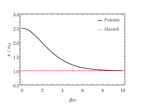
Figure 1: Plot of $\varepsilon/\varepsilon_{M}$ as a function of parameter $\beta m$. It is assumed that the degeneracy degree of Bopp-Podolsky radiation is $g=3$. The energy density of Bopp-Podolsky massive photon gas tends to the ordinary energy density of a massless photon gas as $\beta m$ assumes values larger than $\sim$10.

Fig. 1 shows the plot of $\varepsilon/\varepsilon_{M}$ as a function of the dimensionless parameter $\beta m$. It is assumed $g=3$ for Bopp-Podolsky photon gas. One notices that $\delta\varepsilon$ approaches $g/2$ as $\beta m$ approaches zero, so that $\lim_{\beta m\rightarrow 0}\left(\varepsilon/\varepsilon_{M}\right)=2.5$ $-$ see Eqs. (40) and (42). The same plot also shows that $\delta\varepsilon$ is negligible for large values of $\beta m$ once the curve for $\varepsilon/\varepsilon_{M}$ approaches $1$ from $\beta m\sim 10$ (a condition that is guaranteed for a temperature ten times smaller than the rest mass of the Bopp-Podolsky photon). Ref. Bufalo2012 sets the most restrictive limit for the mass of the photon in Podolsky Generalized Electrodynamics known today, namely

$$m\gtrsim 3.7\times 10^{10}\mbox{eV}\gtrsim 10^{14}\mbox{K}\qquad(\mbox{Bopp-Podolsky})\,;$$ (43)

this is the scale of energy where one expects $\delta\varepsilon$ being relevant. This energy scale corresponds to the early universe, way before the quark-gluon deconfinement. The primeval universe is consistent with the regime where $\beta m\ll 1$ in Bopp-Podolsky theory. This limit and its implication to cosmology are analyzed below.

Eq. (37) may be simplified in the limit $\beta m\ll 1$. The resulting expression for $\ln Z(V,\beta;m)$ is then substituted into Eq. (12) yielding:

$$P\simeq\frac{1}{3}\left(\frac{\pi^{2}}{15}\frac{1}{\beta^{4}}\right)\left[1+\frac{g}{2}\left(1-\frac{15}{4\pi^{2}}\left(\beta m\right)^{2}\right)\right]{\text{ \ \ }}(\beta m\ll 1)\,,$$ (44)

$$\varepsilon\simeq\left(\frac{\pi^{2}}{15}\frac{1}{\beta^{4}}\right)\left[1+\frac{g}{2}\left(1-\frac{5}{4\pi^{2}}\left(\beta m\right)^{2}\right)\right]\qquad(\beta m\ll 1)\,,$$ (45)

which are similar to but not equal to Eqs. (16,17) since they include the Maxwellian contribution to the terms coming from the massive photon.

By inverting Eq. (45) and substituting the result in (44), one gets:

$$P\simeq\frac{\varepsilon}{3}\left(1-4\frac{M^{2}}{\sqrt{\varepsilon}}\right)\qquad(\beta m\ll 1)\,,$$ (46)

if one defines

$$M^{2}=M^{2}(m)\equiv\frac{1}{6}\sqrt{\frac{15}{\pi^{2}}}\frac{\frac{g}{2}}{\sqrt{1+\frac{g}{2}}}\frac{m^{2}}{4}\,\,\,\,\,\,\,\,(\mbox{Bopp-Podolsky})\,.$$ (47)

Eq. (46) is formally the same as Eq. (18), the difference being the definition of parameter $M$: compare Eqs. (47) and (19) keeping in mind that $m$ is very large in Bopp-Podolsky electrodynamics while it is very small in Proca case. This fact guarantees that the steps to calculate $a(t)$ for Bopp-Podolsky radiation are the same as the ones previously followed in de Broglie-Proca’s case, cf. sentences containing Eqs. (20)-(22). Therefore, the scale factor for a Bopp-Podolsky photon gas in the high-energy regime is :

$$a(t)\simeq a_{0}\left\{1+2H_{0}(t-t_{0})\left[1+\frac{M^{2}}{\sqrt{\varepsilon_{0}}}H_{0}(t-t_{0})\right]\right\}^{1/2}$$ (48)

$(\beta m\ll 1)$, just like in de Broglie-Proca’s future universe $-$ see Eq. (22) and interpretation below it. Eq. (48) essentially means that Bopp-Podolsky massive photons may not produce sensible effects in cosmic dynamics. This will be confirmed in the following analysis of the non-approximate solution to Friedmann equations.

The ratio of Eqs. (38) and (39) lead to the parameter of the barotropic equation of state,

$$w=\frac{P}{\varepsilon}=\frac{1}{3}\frac{1}{(1+f)}\,,$$ (49)

where

$$f=f(\beta m)=\frac{\frac{g}{30}(\beta m)^{4}\sum_{k=1}^{\infty}\frac{K_{1}(k\beta m)}{k\beta m}}{1+\frac{g}{10}(\beta m)^{4}\sum_{k=1}^{\infty}\frac{K_{2}(k\beta m)}{(k\beta m)^{2}}}$$ (50)

is the function distinguishing the Maxwellian result ($P=\varepsilon/3$; $f=0$) from Bopp-Podolsky electrodynamics. Fig. 2 shows the plot for $w=w(\beta m)$.

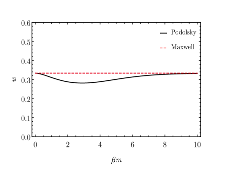
Figure 2: Plot of $w$ as a function of parameter $\beta m$. The dashed line corresponds to $w=1/3$ as expected for a massless photon gas. The continuous line exhibits the behavior of the EOS parameter $w$ for Bopp-Podolsky theory with $g=3$; in this case, $w$ is minimum for $\beta m$ equal to 2.899.

The Maxwell equation of state parameter $w=w_{M}=1/3$ is recovered for both $\beta m\rightarrow 0$ (i.e., $\beta m\ll 1$) and $\beta m\gg 1$; this means that the presence of the massive photon can not sensitively alter cosmic dynamics either in the distant past or in the present/future. In the distant past ($\beta m\ll 1$) the mean thermal energy of the universe is much greater than the rest energy of the massive photon, and the Bopp-Podolsky photon behaves as an ultra-relativistic particle. In the other limit, the condition $\beta m\gg 1$ is satisfied whenever the photon mass is much greater than the temperature $T=\beta^{-1}$; this is a condition fulfilled by the present-day universe whose temperature is $T_{0}\simeq 2.73\text{K}\simeq 2.35\times 10^{-4}\text{eV}$ while $m$ is $3.70\times 10^{10}\text{eV}$ at least $-$ Ref. Bufalo2012 . In spite of the equivalence Maxwell-Podolsky concerning the parameter $w$ in the limits $\beta m\ll 1$ and $\beta m\gg 1$, it is worth mentioning that this is not the case for the energy density: $\varepsilon\rightarrow\varepsilon_{M}$ when $\beta m\gg 1$, but $\varepsilon\rightarrow(5/2)\varepsilon_{M}$ if $\beta m\rightarrow 0$, cf. Fig. 1.

The maximum influence of Bopp-Podolsky massive photons to the equation of state corresponds to the minimum of the curve $w(\beta m)$ in Fig. 2: $w_{\text{min}}\simeq 0.282$ for $\beta m\simeq 2.899$, when the mass is about three times the value of the mean thermal energy of the universe. At this value of $\beta m$,

$$\frac{\Delta w}{w_{M}}=\frac{w_{M}-w_{\text{min}}}{w_{\text{min}}}\simeq 15.4\%$$

and the universe attains its minimum deceleration compared to the one achieved by a massless photon gas. This is true once $\ddot{a}/a\propto(1+3w)$, as one can easily show from Eqs. (1), (2) and $P=w\varepsilon$.

IV Final Remarks

This paper analyzes the effects that a massive photon accommodated by de Broglie-Proca and Bopp-Podolsky theories could produce on cosmic dynamics. The approach is based on the hypothesis of thermal equilibrium which allows the construction of an equation of state for the massive photon gas in each case. It was shown that a barotropic equation of state $P\neq\varepsilon/3$ is produced; this is true for both de Broglie-Proca and Bopp-Podolsky electrodynamics. (This is different from what happens for non-linear electrodynamics in a background field, where $P=\varepsilon/3$ is preserved Akmansoy2014 and no new cosmological phenomenon appears.) However, the departure of the EOS from a Maxwellian form does not guarantee a significant modification in the functional form of the scale factor $a\propto t^{1/2}$ typical of massless radiation.

In particular, the effect of a de Broglie-Proca photon mass is completely negligible for cosmic dynamics when one considers the more realistic context where dark matter and dark energy are present. In fact, as shown in Sect. “de Broglie-Proca cosmology”, from the early universe until a future where $a_{\text{future}}=10^{12}a_{0}$, de Broglie-Proca’s radiation behaves approximately as Maxwell’s: $\varepsilon\sim a^{-4}$. In addition, observations Planck show that the energy density of radiation ($\varepsilon_{\gamma}$) in the present-day universe is ten thousand times smaller then the matter energy density ($\varepsilon_{m}$) today, i.e., $\varepsilon_{\gamma 0}\sim 10^{-4}\varepsilon_{m0}$, regardless of the nature of the cosmic photon gas (either massive or massless). Thus, in a future where the scale factor amounts to $a_{\text{future}}$, one estimates $\varepsilon_{\gamma,\text{future}}\simeq 10^{-16}\varepsilon_{m,\text{future}}$ because $\varepsilon_{m}\sim a^{-3}$: this makes radiation dynamically irrelevant in the face of matter.

If one insists on advancing even further towards the future, considering $a>a_{\text{future}}$, the de Broglie-Proca mass begins to take its toll; $\varepsilon_{\gamma}$ slowly modifies its functional dependence on the scale factor, evolving from $a^{-4}$ to $a^{-3}$ in the future infinity. In this regime ($a\gg 10^{14}a_{0}$) radiation behaves as non-relativistic, but with an initial condition where the radiation energy density is 16 orders of magnitude smaller than matter energy density. Consequently, matter utterly dominates radiation. The situation is deeply aggravated in the presence of some type of dark energy (DE) scaling as $\varepsilon_{\text{DE}}\sim a^{-n}$ where $n<2$; then $\varepsilon_{\gamma,\text{future}}\ll 10^{-14}\varepsilon_{\text{DE,future}}$ rendering the de Broglie-Proca mass even more negligible compared to the dark component.

As seen in Sect. “Bopp-Podolsky cosmology”, Bopp-Podolsky electrodynamics differs from de Broglie-Proca’s in two fundamental ways: the mass of the photon is humongous (instead of been extremely small) and there are derivative terms in the field strength entering the Lagrangian (instead of quadratic terms involving $A^{\mu}$). Someone will argue that these derivative terms lead to the appearance of ghosts, that a theory with such a plague should be immediately discarded as inconsistent. However, some works analyze this issue – e.g., Ref. Kaparulin – and they point to a well-behaved type of ghosts. In fact, Ref. Kaparulin shows that Bopp-Podolsky electrodynamics belongs to a wide class of higher-derivative systems admitting a bounded integral of motion which makes them dynamically stable despite their canonical energy being unbounded. Thermodynamics of Bopp-Podolsky massive photon gas does affect cosmic dynamics, and this occurs for $0\leq\beta m\lesssim 8$ (see Fig. 2). However, this influence is not pronounced: The massive term is not able to produce any sensible deviation of cosmic dynamics from a massless photon gas in the radiation-dominated era. In particular, Bopp-Podolsky radiation can not produce an accelerated expansion in the early universe since its EOS parameter respects: $0.282<w<1/3$.

This paper shows that the maximum influence of Bopp-Podolsky theory on cosmic dynamics takes place for $\beta m\simeq 2.899$. If one chooses the minimum value $m=37\text{GeV}$ in accordance with Eq. (43), this corresponds to $kT\simeq 13\text{GeV}$; i.e., one order of magnitude below the energy scale of electro-weak unification. Notice that the cosmic dynamics for the Bopp-Podolsky radiation was determined at all times in terms of the product $\beta m$: it does not depend directly on the photon mass. In this sense, our work implies that the standard cosmological model does not rule out Bopp-Podolsky massive photon gas as a real possibility. This very fact, along with the success of predictions by generalized quantum electrodynamics Bufalo2011 ; Bufalo2013 ; Bufalo2014 ; Bufalo2012 , motivates the continuing study of Bopp-Podolsky theory. In addition, the massive mode of Bopp-Podolsky photon may interact with charged particles present in the cosmic soup . The resulting dynamics of this interaction is not trivial and a realistic model should take it into account; this might be a suitable subject for future investigation.

- (1) B. S. Ryden, Introduction to Cosmology (Addison-Wesley, 2003).
- (2) V. De Sabbata and M. Gasperini, Introduction to Gravitation (World Scientific, 1985).
- (3) R. K. Pathria and P. D. Beale, Statistical Mechanics, 3rd ed. (Academic Press, 2011).
- (4) L. Tu, J. Luo, and G. T. Gillies, Rep. Prog. Phys. 68, 130 (2004).
- (5) A.S. Goldhaber and M.M. Nieto, Rev. Mod. Phys. 82, 939 (2010).
- (6) L. de Broglie, J. Phys. Radium 3, 422 (1922).
- (7) L. de Broglie, Comptes Rendus Hebd. Séances Acad. Sc. Paris 177, 507 (1923).
- (8) L. de Broglie, La Mécanique Ondulatoire du Photon. Une Nouvelle Théorie de la Lumière (Hermann, 1940).
- (9) A. Proca, J. Phys. Radium 7, 347 (1936).
- (10) F. Bopp, Ann. Phys. (Berlin) 430, 345 (1940).
- (11) B. Podolsky, Phys. Rev. 62, 68 (1942).
- (12) A. Landé and L.H. Thomas, Phys. Rev. 65, 175 (1944).
- (13) R. Aldrovandi and J. G. Pereira, Notes for a course on classical fields (IFT-Unesp, 2012).
- (14) C. A. M. de Melo, B. M. Pimentel and P. J. Pompeia, Nuovo Cim. B 121, 193 (2006).
- (15) D.D. Ryutov, Plasma Phys. Contr. Fus. 40, B429 (2007).
- (16) C. Patrignani et al., Chin. Phys. C 40, 100001 (2016).
- (17) L. Bonetti et al., Phys. Lett. B 757, 548 (2016).
- (18) E. C. G. Stueckelberg, Helv. Phys. Acta 11, 299 (1938).
- (19) H. Ruegg and M. Ruiz-Altaba, Int. J. Mod. Phys. A 19, 3265 (2004).
- (20) E. Allys, P. Peter and Y. Rodríguez, JCAP 02, 004 (2016).
- (21) B. Podolsky and P. Schwed, Rev. Mod. Phys. 20, 40 (1948).
- (22) A. Accioly and H. Mukai, Braz. J. Phys. 28, 35 (1998).
- (23) R. Bufalo, B. M. Pimentel and G. E. R. Zambrano, Phys. Rev. D 83, 045007 (2011).
- (24) R. Bufalo and B. M. Pimentel, Phys. Rev. D 88, 065013 (2013).
- (25) R. Bufalo, B. M. Pimentel and D. E. Soto, Phys. Rev. D 90, 085012 (2014).
- (26) R. R. Cuzinatto et al., Int. J. Mod. Phys. A 26, 3641 (2011).
- (27) C. A. Bonin et al., Phys. Rev. D 81, 025003 (2010).
- (28) R. Bufalo, B. M. Pimentel and G. E. R. Zambrano, Phys. Rev. D 86, 125023 (2012).
- (29) J. Plebansky, Lectures on Non-Linear Electrodynamics (Ed. Nordita, 1968).
- (30) W. Heisenberg and H. Euler, Z. Phys. 98, 714 (1936).
- (31) W. Dittrich and H. Gies, Probing the Quantum Vacuum (Springer, 2000).
- (32) M. Born and L. Infeld, Proc. R. Soc. A 144, 425 (1934).
- (33) M. Born and L. Infeld, Proc. R. Soc. A 147, 522 (1934).
- (34) M. Novello, S. E. P. Bergliaffa and J. Salim, Phys. Rev. D 69, 127301 (2004).
- (35) S. I. Kruglov, Phys. Rev. D 92, 123523 (2015).
- (36) V. A. de Lorenci et al., Phys. Rev. D 65, 063501 (2002).
- (37) M. Novello, A. N. Araujo and J. M. Salim, Int. J. Mod. Phys. A 24, 5639 (2009).
- (38) L. G. Medeiros, Int. J. Mod. Phys. D 21, 1250073 (2012).
- (39) S. Kouwn, P. Oh, and C. Park, Phys. Rev. D 93, 083012 (2016).
- (40) L. Li, Gen. Relativ. Gravit. 48, 1 (2016).
- (41) A. de Felice et al., JCAP 06, 048 (2016).
- (42) Z. Haghani et al., Eur. Phys. J. C 77, 137 (2017).
- (43) R. Utiyama, Phys. Rev. 101, 1597 (1956).
- (44) A. Retinò, A.D.A.M. Spallicci and A. Vaivads, Astropart. Phys. 82, 49 (2016).
- (45) I. S. Gradshteyn and I. M. Ryzhik, Table of Integrals, Series, and Products (Academic Press, 2014).
- (46) R. R. Cuzinatto, C. A. M. de Melo and P. J. Pompeia, Ann. Phys. 322, 1211 (2007).
- (47) C. A. P. Galvao and B. M. Pimentel, Can. J. Phys. 66, 460 (1988).
- (48) P. N. Akmansoy and L. G. Medeiros, Phys. Lett. B 738, 317 (2014).
- (49) Planck Collaboration, Astron. Astrophys. 594, A13 (2015).
- (50) D. S. Kaparulin, S. L. Lyakhovich and A. A. Sharapov, Eur. Phys. J. C 74, 1 (2014).