Developments in maximum likelihood unit root tests

Abstract

The exact maximum likelihood estimate (MLE) provides a test statistic for the unit root test that is more powerful (Fuller, 1996, p. 577) than the usual least squares approach. In this paper a new derivation is given for the asymptotic distribution of this test statistic that is simpler and more direct than the previous method. The response surface regression method is used to obtain a fast algorithm that computes accurate finite-sample critical values. This algorithm is available in the R package mleur that is available on CRAN. The empirical power of the new test is shown to be much better than the usual test not only in the normal case but also for innovations generated from an infinite variance stable distribution as well as for innovations generated from a GARCH$(1,1)$ process.

Keywords: Exact maximum likelihood estimator; Response surface regression; Robust unit root test; Symbolic computation.

1 Introduction

The AR$(1)$ model is widely used in many applications as well as in unit root testing. Modern approaches to the unit root testing problem emphasize the importance of model selection (Pfaff, 2006; Enders, 2010; Patterson, 2010). This paper focuses on testing the null model known as random walk,

$$\nabla z_{t}=a_{t},\quad t=1,2,...,$$ (1)

where $\nabla z_{t}=z_{t}-z_{t-1}$ and $a_{t}$ are independent and normally distributed with mean zero and variance $\sigma^{2}_{a}$. The alternative is assumed to be the stationary AR$(1)$ model with intercept term $\beta$,

$$z_{t}=\beta+\rho z_{t-1}+a_{t},\quad t=1,2,...,$$ (2)

where $|\rho|<1$.

Sometimes it is assumed that $\beta=0$ is known. This case corresponds to the zero-mean AR$(1)$ processes. Both of these models were discussed in the original formulation of the unit root testing problem by Dickey and Fuller (1979) but using the least-squares estimates (LSE) instead of the MLE. The random walk model and the stationary AR$(1)$ alternative provide a suitable family of models for many financial and economic time series. However, as is discussed in §6, other methods are needed if the diagnostic checks reveal that further lagged values need to be included in the model.

Fuller (1996, p. 577) indicates that if the objective is to test the hypothesis of a unit root against the alternative of a stationary process with an unknown mean, the test statistics associated with the exact MLE are more powerful than that with the LSE. The exact MLE referred to is the MLE in the stationary case that corresponds to the alternative hypothesis in the unit root test. Empirical power comparisons among various unit root tests showed that the MLE based tests had much higher power than the Dickey-Fuller (DF) tests (Pantula et al., 1994). Extensions of the MLE method to the ARMA$(1,1)$ and other ARMA processes were discussed by Shin and Fuller (1998).

Fuller (1996, §10.1.3) and Gonzalez-Farias and Dickey (1999) derive the limiting distributions of normalized statistics associated with the exact MLE unit root test under eqns. (1) and (2). This approach is indirect whereas our new derivation in §3 is essentially simpler and more direct. Our method using the Taylor series linearization of the test statistic is carried out through symbolic computer algebra. The exact MLE itself is also derived symbolically through the solution of a cubic equation in §2. The usual approach to the exact MLE using a numerical optimization technique can occasionally have convergence problems. This more direct approach using a symbolic Taylor series linearization is easier to generalize to other problems as well. It is known that computer algebra may handle complicated statistical inference problems (Andrews and Stafford, 2000). There are several examples in time series analysis. Smith and Field (2001) show how a symbolic operator can be used to calculate the joint cumulants of the linear combinations of products of discrete Fourier transforms. Zhang and McLeod (2006) discuss a computer algebra approach to the asymptotic bias and variance coefficients to order $O(1/n)$ for linear estimators in stationary time series. Computer algebra no doubt has many more applications in statistics and time series analysis.

In §4, using response surface curves, we show that the critical values for the MLE test may be efficiently computed. With our fast algorithm, in §5, we demonstrate that the exact MLE test provides not only a sizeable increase in power but also the robustness against alternative specifications for the innovations such as an infinite variance stable distribution and a GARCH$(1,1)$ process. We illustrate how to implement the exact MLE unit root test with two real world examples in §6.

2 Exact MLE

The AR$(1)$ model (2) may also be written,

$$z_{t}-\mu=\rho(z_{t-1}-\mu)+a_{t},t=1,2,...,$$ (3)

where $E(z_{t})=\mu$ and $\beta=\mu(1-\rho)$. When $\mu$ is known, without loss of generality, it is assumed that $\mu=0$. The time series process is stationary if $|\rho|<1$. In the random walk case $\rho=1$ and the process is said to be unit root non-stationary. If $\rho>1$, the process is explosively non-stationary.

Most of unit root tests have been derived under the data generation model,

$$z_{t}-\mu=\rho(z_{t-1}-\mu)+a_{t},t=1,2,...,$$ (4)

where $z_{0}=\mu$ is a fixed value. The only difference between model (3) and (4) is the initial value. The time series represented by (4) is mostly same as that by (3), except that under (4) the process is asymptotically stationary when $|\rho|<1$ and the LSE is the maximum likelihood estimator of $\rho$ conditionally on the initial value.

First consider the zero-mean stationary time series under (3). Its initial value follows a normally distributed random variable with zero mean and a variance of $\sigma^{2}/(1-\rho^{2})$. The exact log-likelihood function of $n$ consecutive observations, $z_{t},t=1,...,n$, may be written as (Minozzo and Azzalini, 1993)

$$l(\sigma^{2},\rho)=-{n\over 2}\log(2\pi)-{n\over 2}\log(\sigma^{2})+{1\over 2}\log(1-\rho^{2})-{1\over 2\sigma^{2}}(a-2\rho b+\rho^{2}c)$$ (5)

where

$$a=\sum\limits_{t=1}^{n}{z_{t}}^{2},\ \ b=\sum\limits_{t=2}^{n}z_{t}z_{t-1},\ \ c=\sum\limits_{t=2}^{n-1}{z_{t}}^{2}.$$ (6)

Maximizing $l(\sigma^{2},\rho)$ in eqn.(5), White (1961), and Minozzo and Azzalini (1993) show that the exact MLE of $\rho$ is the unique real root of the following equation, whose absolute value is less than one.

$${{n-1}\over n}c\rho^{3}-{{n-2}\over n}b\rho^{2}-(c+{a\over n})\rho+b=0.$$ (7)

Dent and Min (1978), Hasza (1980), and Minozzo and Azzalini (1993) point out that the exact MLE may be written as

$$\hat{\rho}=2({{{d_{2}}^{2}-3d_{1}}\over 9})^{1/2}\cos({\theta\over 3}+{4\pi\over 3})-{d_{2}\over 3},$$ (8)

where

$$\theta={\cos^{-1}\{{{9d_{2}d_{1}-27d_{0}-2{d_{2}}^{3}}\over{2({d_{2}}^{2}-3d_{1})^{3/2}}}}\},$$

and

$$d_{2}=-{{n-2}\over{n-1}}{b\over c},\ \ d_{1}=-{n\over{n-1}}(1+{a\over{nc}}),\ \ d_{0}={n\over{n-1}}{b\over c}.$$

Using Mathematica (Wolfram, 1999), the cubic equation (7) is easily solved and the exact MLE $\hat{\rho}$ may be expressed as the ratio of complex polynomials,

$$\hat{\rho}= {(n-2)b}/3c(-1+n)+((1-i\sqrt{3})$$

$$(-b^{2}(-2+n)^{2}+3c(-1+n)(-a-cn)))/(32^{2/3}c(1-n)$$

$$(16b^{3}-18abc-24b^{3}n+27abcn+9bc^{2}n+12b^{3}n^{2}-9abcn^{2}$$

$$-27bc^{2}n^{2}-2b^{3}n^{3}+18bc^{2}n^{3}+(((16b^{3}-18abc-24b^{3}n+27abcn$$

$$+9bc^{2}n+12b^{3}n^{2}-9abcn^{2}-27bc^{2}n^{2}-2b^{3}n^{3}+18bc^{2}n^{3})^{2}+4(-b^{2}(-2+n)^{2}$$

$$+3c(-1+n)(-a-cn))^{3}))^{1/2})^{1/3})-1/(62^{1/3}c(1-n))$$

$$((1+i\sqrt{3})(16b^{3}-18abc-24b^{3}n+27abcn+9bc^{2}n+12b^{3}n^{2}$$

$$-9abcn^{2}-27bc^{2}n^{2}-2b^{3}n^{3}+18bc^{2}n^{3}+(((16b^{3}-18abc-$$

$$-24b^{3}n+27abcn+9bc^{2}n+12b^{3}n^{2}-9abcn^{2}-27bc^{2}n^{2}-2b^{3}n^{3}$$

$$+18bc^{2}n^{3})^{2}+4(-b^{2}(-2+n)^{2}+3c(-1+n)(-a-cn))^{3}))^{1/2})^{1/3})$$

where $i=\sqrt{-1}$, and $a$, $b$ and $c$ are defined in (6).

For a stationary AR(1) process with an unknown mean under (3), there are two mean correction methods: sample mean correction and the maximum likelihood mean estimation. It is well known that for ARMA$(p,q)$ model, the sample mean is asymptotically efficient (Brockwell and Davis, 1987, §7.1). The exact MLE for the $\mu$ may be obtained iteratively as in McLeod and Zhang (2008) but in the AR$(1)$ case the sample mean has close to 100% efficiency in finite samples (McLeod and Zhang, 2008, Table 3). For speed and convenience we may just consider the sample mean estimator in eqn. (3). That is, the exact MLE is the $\hat{\rho}$ described above with $z_{t}-{\overline{z}}_{n}$ ($t=1,...,n$) replacing $z_{t}$ where ${\overline{z}}_{n}$ is the sample mean, which is denoted as $\hat{\rho}_{\mu}$.

Under the stationary alternative, the exact MLE and the LSE have the same limiting distribution (Brockwell and Davis, 1987, §8) but this is not the case under the non-stationary null hypothesis eqn. (1). The next section provides a new derivation of this distribution.

3 Computer Algebra Derivations to Limiting Distributions

In the unit root case, $\rho=1$, we consider the random walk

$$z_{t}=z_{t-1}+a_{t},\quad t=1,2,...,$$ (9)

where $\{a_{t}\}$ is a sequence of IID random variables with mean 0 and finite variance $\sigma_{a}^{2}>0$.

Fixed $z_{0}=0$, the random walk process may be generated by

$$z_{t}=\sum\limits_{j=1}^{t}{a_{j}}.$$ (10)

For the zero-mean case, the normalized and pivotal type statistics may be written as

$$\hat{\delta}=n(\hat{\rho}-1)$$ (11)

where $\hat{\rho}$ is described in §2, and

$$\hat{\tau}={1\over{\hat{\sigma}}}(\sum\limits_{t=2}^{n}{z^{2}_{t-1}})^{1/2}(\hat{\rho}-1)$$ (12)

where

$$\hat{\sigma}^{2}=(n-2)^{-1}\sum\limits_{t=2}^{n}(z_{t}-\hat{\rho}z_{t-1})^{2}.$$

For the unknown mean case, the normalized statistic may be written as

$$\hat{\delta}_{\mu}=n(\hat{\rho}_{\mu}-1)$$ (13)

where $\hat{\rho}_{\mu}$ is described in §2, and the corresponding pivotal statistic may be written by

$$\hat{\tau}_{\mu}=\hat{\sigma}_{\mu}^{-1}(\sum\limits_{t=2}^{n}{(z_{t-1}-{\overline{z}}_{n})^{2}})^{1/2}(\hat{\rho}_{\mu}-1),$$ (14)

where

$$\hat{\sigma}_{\mu}^{2}=(n-3)^{-1}\sum\limits_{t=2}^{n}(z_{t}-{\overline{z}}_{n}-\hat{\rho}_{\mu}(z_{t-1}-{\overline{z}}_{n}))^{2}.$$

The limiting distributions of statistics in eqns. (11), (12), (13) (14) are given in Theorems 1 and 2 below.

Theorem 1.

Under a random walk (9),

$$n(\hat{\rho}_{\mu}-1)\stackrel{{\scriptstyle D}}{{\longrightarrow}}\frac{1}{2}\left(\mathfrak{C}_{\mu}-\sqrt{\mathfrak{C}_{\mu}^{2}-4\mathfrak{C}_{\mu}+2\mathfrak{B}_{\mu}}\right),$$ (15)

$$\hat{\tau}_{\mu}\stackrel{{\scriptstyle D}}{{\longrightarrow}}\frac{\sqrt{\mathfrak{A}_{\mu}}}{2}\left(\mathfrak{C}_{\mu}-\sqrt{\mathfrak{C}_{\mu}^{2}-4\mathfrak{C}_{\mu}+2\mathfrak{B}_{\mu}}\right),$$ (16)

where

$$\mathfrak{A}_{\mu}=\int_{0}^{1}W^{2}(t)\,dt-\left(\int_{0}^{1}W(t)\,dt\right)^{2},$$

$$\mathfrak{B}_{\mu}=\mathfrak{A}_{\mu}^{-1}\left(\left(\int_{0}^{1}W(t)\,dt\right)^{2}+\left(W(1)-\int_{0}^{1}W(t)\,dt\right)^{2}\right),$$

$$\mathfrak{C}_{\mu}=\mathfrak{A}_{\mu}^{-1}\left(\frac{1}{2}\left(W^{2}(1)-1\right)-W(1)\int_{0}^{1}W(t)\,dt+\left(\int_{0}^{1}W(t)\,dt\right)^{2}\right),$$

and $\{W(t),\ 0\leq t\leq 1\}$ is a standard Wiener process.

Theorem 2.

Under a random walk (9),

$$n(\hat{\rho}-1)\stackrel{{\scriptstyle D}}{{\longrightarrow}}\frac{1}{2}\left(\mathfrak{C}-\sqrt{\mathfrak{C}^{2}-4\mathfrak{C}+2\mathfrak{B}}\right),$$ (17)

$$\hat{\tau}\stackrel{{\scriptstyle D}}{{\longrightarrow}}\frac{\sqrt{\mathfrak{A}}}{2}\left(\mathfrak{C}-\sqrt{\mathfrak{C}^{2}-4\mathfrak{C}+2\mathfrak{B}}\right),$$ (18)

where

$$\mathfrak{A}=\int_{0}^{1}W(t)^{2}\,dt,$$

$$\mathfrak{B}=\mathfrak{A}^{-1}W(1)^{2},$$

$$\mathfrak{C}=\mathfrak{A}^{-1}{\frac{1}{2}\left(W^{2}(1)-1\right)}$$

and $\{W(t),\ 0\leq t\leq 1\}$ is a standard Wiener process.

To fix ideas, below is demonstrated how Mathematica helping to prove the limiting distribution of $n(\hat{\rho}_{\mu}-1)$, eqn. (15) in Theorem 1 .

$\hat{\rho}_{\mu}$ may be further simplified as follows:

$$\hat{\rho}_{\mu}=-\frac{(n-2)G}{3(1-n)}+\frac{(1-i\sqrt{3})u}{2^{2\over 3}3(1-n)(v+\sqrt{v^{2}+4u^{3}})^{1\over 3}}-{{(1+i\sqrt{3})(v+\sqrt{v^{2}+4u^{3}})^{1\over 3}}\over{2^{1\over 3}6}(1-n)}$$

where

$$u= -(n-2)^{2}G^{2}+3(1-n)(H+n),$$

$$v= 16G^{3}-18GH-24G^{3}n+27GHn+9Gn$$

$$+12G^{3}n^{2}-9GHn^{2}-27Gn^{2}-2G^{3}n^{3}+18Gn^{3}$$

where

$$G=b/c,\ \ H=a/c$$ (19)

where $a$, $b$ and $c$ are defined in (6) with $z_{t}-{\overline{z}}_{n}$ ($t=1,...,n$) replacing $z_{t}$. The limiting distributions of $G$ and $H$ are given in the following lemma.

Lemma 1.

Under a random walk (9),

$$(c/(\sigma^{2}n^{2}),n(H-1),n(G-1))\stackrel{{\scriptstyle D}}{{\longrightarrow}}(\mathfrak{A}_{\mu},\mathfrak{B}_{\mu},\mathfrak{C}_{\mu})$$ (20)

where $\mathfrak{A}_{\mu}$, $\mathfrak{B}_{\mu}$, $\mathfrak{C}_{\mu}$ are defined in Theorem 1.

A detailed proof of Lemma 1 can be found in Appendix 8.

Proof of eqn. (15) in Theorem 1.

Let $W=n(G-1)$ and $X=n(H-1)$. Lemma 1 implies that $W=O_{p}(1)$ and $X=O_{p}(1)$. $\hat{\rho}_{\mu}$ can be considered as a function of $1/n$ with $1+W/n$ and $1+X/n$ replacing $G$ and $H$. In order to obtain the limit distribution of $\hat{\rho}_{\mu}$, taking $\hat{\rho}_{\mu}$ with one-term Taylor expansion with respect to $1/n$ at zero,

$$\hat{\rho}_{\mu}=1+\frac{1}{2n}\left(W-\sqrt{W^{2}-4W+2X}\right)+\frac{1}{n^{2}}R_{n}(W,X).$$ (21)

where $\sup_{n\geq 1}|R_{n}(W,X)|\leq C(W,X)$ that is a continuous function of $W$ and $X$. Below is a Mathematica script and its output for deriving eqn (21).

In[1]:= u = -(n-2)^2G^2+3(1-n)(H+n);
In[2]:= v = 16 G^3-18 G H - 24 G^3 n+27 G H n + 9G n + 12 G^3 n^2
            -9 G H n^2-27 G n^2-2 G^3 n^3+18 G n^3;
In[3]:= rho = -(-2+n)G/(3(1-n))
        +((1-i Sqrt[3])(u))/(3 2^(2/3)(1-n)(v+Sqrt[v^2+4u^3])^(1/3))
        -1/(6 2^(1/3)(1-n))((1+i Sqrt[3])(v+Sqrt[v^2+4u^3])^(1/3));
In[4]:= G = 1 + W/n; H = 1 + X/n; n = 1/z;
        Simplify[Series[rho, {z, 0, 1}]]

and the output of the final input is

Out[4]= 1+1/2(W+i(4W-W^2-2X)^(1/2))z+O[z]^2

which leads to eqn. (21). Following the fact that $W=O_{p}(1)$, $X=O_{p}(1)$ and the continuity of $C(W,X)$,

$$\frac{1}{n}R_{n}(W,X)\stackrel{{\scriptstyle P}}{{\longrightarrow}}0.$$

By Lemma 1,

$$(W,X)\stackrel{{\scriptstyle D}}{{\longrightarrow}}(\mathfrak{C}_{\mu},\mathfrak{B}_{\mu}).$$

Thus applied the continuous mapping theorem described in Appendix 8 and the Slutsky’s theorem to eqn. (21), enq. (15) is obtained. ∎

The limiting distributions of $\hat{\tau}_{\mu}$, $\hat{\rho}$, and $\hat{\tau}$ in eqns. (16) - (18) can be very similarly derived.

Fuller (1996, Theorem 10.1.10 and Corollary 10.1.10) show that eqn. (15) and eqn. (17) hold, which indicates that the computer algebra derivations implemented here are appropriate. Other than the normalized statistics, eqns. (16) and (18) show the limiting distributions on the unit root boundary of pivotal statistics for both zero-mean and unknown mean cases.

4 Methods of Implementing the Test

The asymptotic distribution may be evaluated by computer simulation methods for Brownian motion. Such methods are discussed in the book by Iacus (2008). Then this asymptotic distribution could be used to obtain critical values and/or p-values for the test. As we will show below, this method will not work unless the series length is very long.

The simplest approach is to use a Monte-Carlo test. Under general conditions this approach provides an accurate test that can be efficiently computed using parallel processing capabilities found on many modern computer environments. For example, the necessary steps are outlined below for the normalized test:

1) simulate $M$ random walks under (1) with the length of $n$ and compute the simulated testing statistic sample, $n({\hat{\rho}}^{1}_{\mu}-1)$, $n({\hat{\rho}}^{2}_{\mu}-1)$, …, $n({\hat{\rho}}^{M}_{\mu}-1)$;
2) compute the observed testing statistic value for the given time series $\{z_{t}\}$, $n({\hat{\rho}}^{0}_{\mu}-1)$;
3) count the number of times $k$ that the simulated test statistic $n(\hat{\rho}^{i}_{\mu}-1)$ ($i=1,...,M$) is less than or equal to the observed test statistic $n({\hat{\rho}}^{0}_{\mu}-1)$;
4) compute the p-value as $(k+1)/(M+1)$.

Instead of using independent normal random variables to generate the random walks in Step 1), we could use a bootstrap sample of the residuals. This test has been implemented in the function mctest in our R package for MLE unit root tests (A. I. McLeod and Zhang, 2011).

An even more computationally efficient approach is to use response surface regression (MacKinnon, 2002) to estimate the quantile functions for the exact distribution. The response surface regressions are of the form,

$$Q^{\alpha}(n)=\theta_{\infty}+{\theta_{1}}/n+{\theta_{2}}/n^{2}+{\theta_{3}}/n^{3}+\epsilon,$$

where $Q^{\alpha}(n)$ is an $\alpha$ percentile of the finite sample distribution that is estimated using $N$ replications and $\epsilon$ is an error term. The curve was fit with the massive cluster computer SHARCNET utilizing 221 compute nodes for about ten hours. Thirty-six series lengths $n$ used were 20, (5), 100, (20), 300, (50), 500, (100), 1000. For each series length $N=200000$ replications were done and this as repeated $M=100$ times. From this the mean and variance of each percentile were estimated and used in a weighted least squares regression to obtain the final fitted regression. The weighted least squares approach is needed to account for heteroskedasticity in the error terms.

In the case of the model specified in eqns. (1) and (2), the critical values for the test statistic $\hat{\tau}_{\mu}$ given in eqn. (14) are:

$$\hat{Q}^{\alpha}(n)=\left\{\begin{array}[]{rl}-3.110-4.652/n-51.466/n^{2}&\mbox{1\% point}\\ -2.531-2.062/n-17.529/n^{2}&\mbox{5\% point}\\ -2.233-1.219/n-8.178/n^{2}&\mbox{10\% point}\end{array}\right.$$ (22)

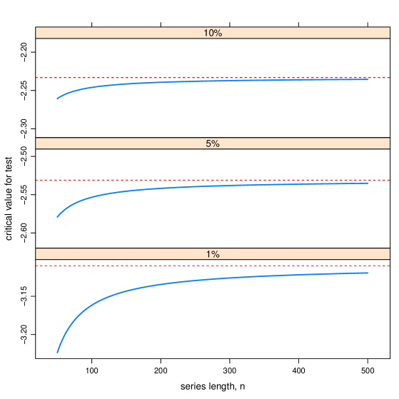
Figure 1: The 1%, 5% and 10% critical values for the MLE test statistic $\hat{\tau}_{\mu}$

Figure 1 below illustrates these curves for series lengths up to 500. The dashed line shows the critical point from the asymptotic distribution. It is seen that a reasonably large sample is needed to obtain accurate critical values using the asymptotic distribution. The y-axis each panel is scaled so scaling unit is the same. This scaling reveals the critical values corresponding 10% converge more quickly while the 1% critical values converge slowly.

Extensive simulation experiments were performed for a variety of series lengths, $n$, and parameters, $\rho$, to check that the p-values produced by the Monte-Carlo method agreed with that produced by the critical values from eqn. (22).

Implementing the explicit expression of the exact MLE derived in §2 and the critical value equations such as eqns. (22), our R function mleur for the MLE unit root tests is available in our R package mleur (A. I. McLeod and Zhang, 2011).

5 Power Comparisons

We investigated the power of the MLE unit root tests under various types of innovations in comparison with that of the standard Dickey-Fuller test. Under our null model (1), and alternative model (2) or (3), the unknown mean case is more realistic than the known mean case. Thus the MLE unit root test was implemented with the sample mean correction in the normalized form $n(\hat{\rho}_{\mu}-1)$ or the pivotal form $\hat{\tau}_{\mu}$, denoted by MLEn or MLEp respectively. In R the standard Dickey-Fuller test is implemented in several packages and usually the pivotal form of test statistic is used. We used the implementation of the Dickey-Fuller pivotal test for the same model as (1) and (2) with an unknown mean or interpret in the R package urca by Pfaff (2010), represented by DF in this paper. The function GetPower for making such power comparisons is given in our package (A. I. McLeod and Zhang, 2011)

In constructing critical value eqns. (22), the simulated series were assumed to be Gaussian. But since the asymptotic distribution only relies on the assumption that the innovations are independent with mean zero and finite variance $\sigma_{a}^{2}$, it is plausible that the critical values given in eqns. (22) may also be applicable for other non-normal distributions with finite variance. In fact, using our R function GetPower, we found no difference from the normal distribution results with Student-t on 5 degrees of freedom. A more challenging question is how well these results continue to hold when these assumptions are not met as in the case of infinite variance distributions, or series exhibiting conditional heteroscedasticity and non-linear dependence. To answer this question, a portion of our simulation results is shown in Table 1. $25,000$ replications were done for series of lengths $n=30,70,100,200$ and parameters $\rho=0.65,0.85,0.9,0.95,1.0$ for the innovations generated by a stable distribution and a GARCH model described in the following. With so many replications the 95% margin-of-error (MOE) was about 0.0062 or 0.62 in percentage terms. This computations took less than 3 hours on a multicore PC.

The random variable $Z$ has a stable distribution with index $\alpha$, scale $\sigma>0$, skewness $|\beta|<1$ and location $\mu\in{\cal R}$ if its characteristic function is given by,

$${{\rm~{}E\,}}(e^{itZ})=\left\{\begin{array}[]{cl}\exp\left\{-\sigma|t|^{\alpha}\,\left(1-i\beta\ \ \mbox{sgn}(t)\,\tan\frac{\pi\alpha}{2}\right)+\,i\mu t\right\}&\mbox{if}\ \alpha\neq 1\\ \\ \exp\left\{-\sigma|t|\,\left(1+i\beta\frac{2}{\pi}\ \ \mbox{sgn}(t)\,\log|t|\right)+\,i\mu t\right\}&\mbox{if}\ \alpha=1,\end{array}\right.$$

where

$$\mbox{sgn}(t)=\left\{\begin{array}[]{rl}1&\mbox{if}\quad t>0\\ 0&\mbox{if}\quad t=0\\ -1&\mbox{if}\quad t<0.\end{array}\right.$$

Since it has been suggested that many financial time series appear to have a stable distribution with $\alpha$ in the range $(1.35,1.75)$, $\alpha$ was set to $1.5$ for our simulations. Also, $\sigma=1$, $\beta=0$, and $\mu=0$.

A GARCH($1,1$) sequence $a_{t},t=\ldots,-1,0,1,\ldots$ is of the form

$$a_{t}=\sigma_{t}\epsilon_{t}$$

and

$$\sigma_{t}^{2}=\omega+\alpha_{1}a^{2}_{t-1}+\beta_{1}\sigma_{t-1}^{2},$$

where we took $\epsilon_{t}$ to be independent standard normal, $\omega=10^{-6},\alpha_{1}=0.2$ and $\beta_{1}=0.7$. The parameters were chosen to approximate models that have been used in actual applications.

Table 1 shows that there can be substantial difference in power between the MLE unit root test and the Dickey-Fuller tests not only in the normal case but also for innovations generated from an infinite variance stable distribution as well as for innovations generated from a GARCH(1,1) process. It is observed that the size of the test is slightly inflated for the non-normal case, so this needs to be taken into account in the power comparison. In general it appears that the pivotal form of the test statistic, MLEp, is preferable to the normalized form, MLEn. MLEp is just as robust as MLEn and has slightly better power.

Further empirical power analysis may easily be carried out similarly with our R function GetPower.

6 Illustrative Applications

In actual applications, it is recommended that diagnostic checks be done for residual autocorrelation. If there is significant autocorrelation in the residuals of the fitted AR(1) model then other methods such as the augmented Dickey-Fuller test must be used. The model building procedure needed for this Dickey-Fuller test family is discussed by Pfaff (2006) and is available in the R package urca (Pfaff, 2010). Our R package mleur (A. I. McLeod and Zhang, 2011) provides suitable model diagnostic checks for applying the MLE root test and is used in the applications discussed below. R scripts to generate the analyses reported below are available in our package documentation.

6.1 Velocity of money

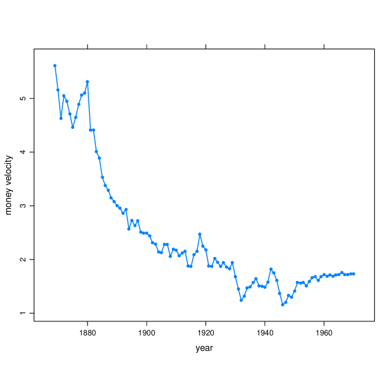
Figure 2: Time series plot for money velocity

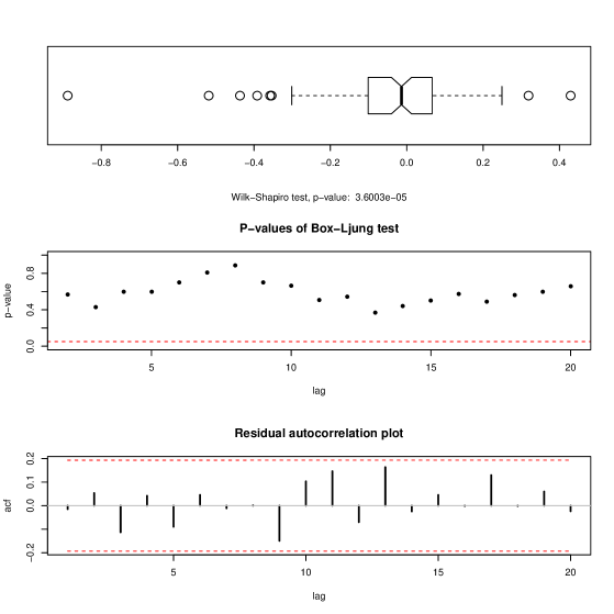
Figure 3: Diagnostic plots for money velocity time series

The time series plot for the velocity of money in the U.S. 1869-1970 is shown in Figure 2. From the plot we see the series has historically exhibited a strong stochastic trends characteristic of random walk behavior. No doubt with modern emphasis on fiscal policies to control inflation the series has stabilized. But just for a numerical illustration of the difference in the unit root tests we will compare the maximum likelihood and least squares or Dickey-Fuller tests. The first step in the analysis is the check that the fitted model is adequate and that no additional lags are required. Figure 3 shows the diagnostic checks for this data. The residuals appear non-normal but in view of the simulation results this is not a concern. Most importantly no evidence of residual autocorrelation is found in the fitted AR(1) model. Applied the unit root tests, the pivotal test statistics for the MLE and DF tests were respectively $-0.26$ and $-3.28$. The MLE test is not even close to being significant at the 10% level while the DF test has a p-value between 5% and 1%. The MLE unit root test gives a result that appears to be more in line with the overall impression of strong stochastic trends exhibited in Figure 2. Even though the length of the series was $102$, there is a considerable difference in the conclusion between the two methods.

6.2 Bond yield differences

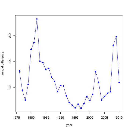
Figure 4: Time series plot of difference in bond yields

The annual difference in Mood’s BAA and AAA corporate bond yields from 1976 to 2010 is shown in Figure 4. From the diagnostic check plots, we conclude that there is no significant autocorrelation in the residuals and so the AR(1) may be fit. The DF test is not significant at 10% whereas the MLE test does reject at the 10% level. This is not surprising in view of the empirical power computations.

7 Summary

In this paper we presented a new derivation of the asymptotic distribution for the MLE unit root test utilizing computer algebra to obtain an explicit expression for the MLE and a Taylor series linearization for the test statistic. This technique is no doubt applicable in other situations where the manual derivation is difficult.

An efficient computational method based on the response surface curves has been implemented to obtain critical values of the MLE test statistics. An empirical power study has demonstrated that not only does the MLE procedure outperform the LSE in the Gaussian case but also for fat-tailed distributions, infinite variance distributions, and for weak dependence as exhibited in a GARCH$(1,1)$ process. The R package mleur based on the developments in this paper is available on CRAN.

Two illustrative applications of the test demonstrate that unit root testing also requires diagnostic checking. It is important for proper applications that there be no residual autocorrelation present in the fitted AR$(1)$ model.

ACKNOWLEDGEMENTS

The authors would like to thank the Editor for his encouragement and also two referees for their helpful suggestions and comments. The authors research was supported by Natural Sciences and Engineering Research Council of Canada (NSERC).

8 Appendix

First we state the Donsker’s theorem (Billingsley, 1999). Let $\{a_{t}\}$ be a sequence of IID random variables with mean 0 and finite variance $\sigma^{2}>0$, $z_{t}=\sum_{j=1}^{t}a_{j}$ and $z_{0}=0$. Then

$$\left\{\frac{z_{[nt]}}{\sqrt{n}\sigma},\ 0\leq t\leq 1\right\}\stackrel{{\scriptstyle D}}{{\longrightarrow}}\{W(t),\ 0\leq t\leq 1\}$$

in the Skorokhod space $D[0,\ 1]$ with $J_{1}$ topology, where $[x]$ denotes the integer part of $x$. One of the important applications of the Donker’s theorem is the following continuous mapping theorem. If $f(\cdot)$ is a continuous functional on $[0,\ 1]$, then

$$f\left(\frac{z_{[nt]}}{\sqrt{n}\sigma}\right)\stackrel{{\scriptstyle D}}{{\longrightarrow}}f(W(t)).$$

Proof of Lemma 1.

We have

$$\frac{\bar{z}_{n}}{\sqrt{n}}=\int_{0}^{1}\frac{z_{[nt]}}{\sqrt{n}}\,dt+\frac{z_{n}}{n\sqrt{n}}.$$

By the Donsker’s theorem

$$\frac{\bar{z}_{n}}{\sqrt{n}}\stackrel{{\scriptstyle D}}{{\longrightarrow}}\sigma\int_{0}^{1}W(t)\,dt.$$

Similarly,

$$\frac{1}{n^{2}}\sum_{t=1}^{n-1}z_{t}^{2}=\int_{0}^{1}\left(\frac{z_{[nt]}}{\sqrt{n}}\right)^{2}\,dt\stackrel{{\scriptstyle D}}{{\longrightarrow}}\sigma^{2}\int_{0}^{1}W^{2}(t)\,dt.$$

It can be shown that

$$c=\sum_{t=2}^{n-1}\left(z_{t}-\bar{z}_{n}\right)^{2}=\sum_{t=1}^{n-1}z_{t}^{2}-z_{1}^{2}-(n+2)\bar{z}_{n}^{2}+2\bar{z}_{n}(z_{1}+z_{n}).$$ (23)

By some simple algebra steps,

$$b-c = \sum_{t=1}^{n-1}(z_{t+1}-z_{t})(z_{t}-\bar{z}_{n})+(z_{1}-\bar{z}_{n})^{2}$$

$$= \frac{1}{2}z_{n}^{2}-\frac{1}{2}\sum_{t=1}^{n}a_{t}^{2}-\bar{z}_{n}\sum_{t=2}^{n}a_{t}+(z_{1}-\bar{z}_{n})^{2},$$

that is,

$$\frac{b-c}{n}=\frac{1}{2}\left(\frac{z_{n}}{\sqrt{n}}\right)^{2}-\frac{1}{2n}\sum_{t=1}^{n}a_{t}^{2}-\frac{\bar{z}_{n}}{\sqrt{n}}\frac{z_{n}}{\sqrt{n}}+\frac{\bar{z}_{n}}{\sqrt{n}}\frac{a_{1}}{\sqrt{n}}+\left(\frac{z_{1}}{\sqrt{n}}-\frac{\bar{z}_{n}}{\sqrt{n}}\right)^{2}.$$ (24)

Moreover

$$\frac{a-c}{n}=\left(\frac{z_{1}}{\sqrt{n}}-\frac{\bar{z}_{n}}{\sqrt{n}}\right)^{2}+\left(\frac{z_{n}}{\sqrt{n}}-\frac{\bar{z}_{n}}{\sqrt{n}}\right)^{2}.$$ (25)

Since

$$\frac{b-c}{n}=n(G-1)(\frac{c}{n^{2}})$$

and

$$\frac{a-c}{n}=n(H-1)(\frac{c}{n^{2}}),$$

where $G$ and $H$ are defined in eqn (19). Eqns. (23), (24), and (25) imply that

$$(\frac{c}{\sigma^{2}n^{2}},n(H-1),n(G-1))=f(\frac{z_{[nt]}}{\sqrt{n}\sigma})+o_{p}(1),$$

where $f$ is a functional. Hence by the continuous mapping theorem described above and Slutsky’s theorem,

$$(\frac{c}{\sigma^{2}n^{2}},n(H-1),n(G-1))\stackrel{{\scriptstyle D}}{{\longrightarrow}}f(W(t)).$$

Applied the Cramer-Rao device, we find the marginal distributions as

$$\frac{c}{\sigma^{2}n^{2}}\stackrel{{\scriptstyle D}}{{\longrightarrow}}\int_{0}^{1}W^{2}(t)\,dt-\left(\int_{0}^{1}W(t)\,dt\right)^{2}=\mathfrak{A}_{\mu},$$

$$n(G-1)\stackrel{{\scriptstyle D}}{{\longrightarrow}}\mathfrak{A}_{\mu}^{-1}\left(\frac{1}{2}\left(W^{2}(1)-1\right)-W(1)\int_{0}^{1}W(t)\,dt+\left(\int_{0}^{1}W(t)\,dt\right)^{2}\right)=\mathfrak{C}_{\mu},$$

and

$$n(H-1)\stackrel{{\scriptstyle D}}{{\longrightarrow}}\mathfrak{A}_{\mu}^{-1}\left(\left(\int_{0}^{1}W(t)\,dt\right)^{2}+\left(W(1)-\int_{0}^{1}W(t)\,dt\right)^{2}\right)=\mathfrak{B}_{\mu}.$$

∎

		normal			stable			GARCH(1,1)
$n$	$\rho$	DF	MLEn	MLEp	DF	MLEn	MLEp	DF	MLEn	MLEp
30	0.65	39.8	56.5	59.6	36.5	55.7	59.4	42.0	56.2	59.0
70	0.65	97.6	99.8	99.7	97.7	98.6	98.1	95.6	98.9	98.8
100	0.65	100.0	100.0	100.0	99.7	99.3	99.1	99.7	100.0	99.9
200	0.65	100.0	100.0	100.0	99.9	99.7	99.6	100.0	100.0	100.0
30	0.85	12.1	16.6	18.3	11.6	12.5	13.6	14.1	18.3	20.0
70	0.85	37.4	55.1	57.4	33.6	53.9	57.0	39.7	55.9	57.8
100	0.85	63.2	83.2	84.2	65.2	84.3	84.6	64.5	81.4	82.1
200	0.85	99.6	100.0	100.0	99.4	98.9	98.4	98.7	99.7	99.6
30	0.90	8.4	10.7	11.9	8.9	8.3	8.9	9.8	11.8	13.1
70	0.90	19.4	29.8	31.4	17.4	24.6	26.8	22.0	32.0	33.7
100	0.90	33.3	51.0	52.8	29.7	49.4	52.8	36.3	51.9	53.5
200	0.90	86.8	97.2	97.0	89.3	95.7	94.8	84.3	94.7	94.7
30	0.95	6.7	7.6	8.3	6.5	5.5	5.7	7.8	8.1	9.1
70	0.95	9.2	12.5	13.3	9.0	9.5	9.9	11.0	14.7	15.4
100	0.95	12.5	19.0	19.8	11.8	14.2	15.1	14.6	21.2	22.0
200	0.95	32.5	51.1	52.5	28.9	47.7	50.7	36.0	52.6	53.9
30	1.00	5.5	4.9	5.5	6.3	4.3	4.4	7.0	6.1	6.7
70	1.00	5.2	5.1	5.3	6.0	3.7	3.7	7.0	6.1	6.4
100	1.00	5.0	5.3	5.6	6.0	3.9	3.8	6.7	6.3	6.3
200	1.00	4.9	4.8	4.9	5.9	3.8	3.8	6.2	6.2	6.3

Table 1: Empirical power of 5% unit root tests based on 25,000 simulations using innovations from various distributions. Tests were Dickey-Fuller (DF), MLE normalized (MLEn), and MLE pivotal (MLEp). The distributions used were standard normal, stable distribution with index parameter 1.5, and a GARCH$(1,1)$ process. The 0.95 level MOE for the table percentage is 0.62

References

- A. I. McLeod and Zhang (2011) A. I. McLeod, H. Y. and Y. Zhang (2011). Fmleur: Maximum Likelihood Unit Root Test. R package version 1.0-1.
- Andrews and Stafford (2000) Andrews, D. F. and J. E. Stafford (2000). Symbolic Computation for Statistical Inference. Oxford.
- Billingsley (1999) Billingsley, P. (1999). Convergence of Probability Measures. New York: John Wiley & Sons, Inc.
- Brockwell and Davis (1987) Brockwell, P. J. and R. A. Davis (1987). Time Series: Theory and Methods. New York: Springer-Verlag.
- Dent and Min (1978) Dent, W. and A. S. Min (1978). A monto carlo study of autoregressive integrated moving average processes. Journal of Econometrics 7, 23–55.
- Dickey and Fuller (1979) Dickey, A. D. and W. A. Fuller (1979). Distribution of the estimators for autoregressive time series with a unit root. Journal of the American Statistical Assiciation 74, 427–431.
- Enders (2010) Enders, W. (2010). Applied Econometric Time Series (3rd ed.). New York: John Wiley and Sons.
- Fuller (1996) Fuller, W. A. (1996). Introduction to Statistical Time Series. New York: Wiley.
- Gonzalez-Farias and Dickey (1999) Gonzalez-Farias, G. M. and D. A. Dickey (1999). Unit root test: An unconditional maximum likelihood approach. Boletin de la Sociedad Matematica Mexicana 5, 199–221.
- Hasza (1980) Hasza, D. P. (1980). A note on the maximum likelihood estimation for the first-order autoregressive processes. ommunications in Statistics: Theory and Methods 13, 1411–15.
- Iacus (2008) Iacus, S. M. (2008). Simulation and Inference for Stochastic Differential Equations: With R Examples. New York: Springer Science+Business Media, LLC.
- MacKinnon (2002) MacKinnon, J. (2002). The International Series in Engineering and Computer Science, Volume 541, Chapter Computing Numerical Distribution Functions in Econometrics, pp. 455–471. Springer-Verlag.
- McLeod and Zhang (2008) McLeod, A. and Y. Zhang (2008). Faster arma maximum likelihood estimation. Computational Statistics and Data Analysis 52(4), 2166–2176.
- Minozzo and Azzalini (1993) Minozzo, M. and A. Azzalini (1993). On the unimodality of the exact likelihood function for normal ar(2) series. Journal of Time Series Analysis 14, 497–510.
- Pantula et al. (1994) Pantula, S. G., G. Gonzalez-Farias, and W. A. Fuller (1994). A comparison of unit-root test criteria. Journal of Business & Economic Statistics 12(4), 449–459.
- Patterson (2010) Patterson, K. (2010). A Primer for Unit Root Testing. London: Palgrave.
- Pfaff (2006) Pfaff, B. (2006). Analysis of Integrated and Cointegrated Time Series with R. New York: Springer.
- Pfaff (2010) Pfaff, B. (2010). urca: Unit root and cointegration tests for time series data. R package version 1.2-5.
- Shin and Fuller (1998) Shin, D. W. and W. Fuller (1998). Unit root tests based on unconditional maximum likelihood estimation for the autoregressive moving average. Journal of Time Series Analysis 19(5), 591 –599.
- Smith and Field (2001) Smith, B. and C. Field (2001). Symbolic cumulant calculations for frequency domain time series. Statistics and Computing 11, 75–82.
- White (1961) White, J. S. (1961). Asymptotic expansions for the mean and variance of the serial correlation coefficient. Biometrika 48, 85–94.
- Wolfram (1999) Wolfram, S. (1999). The Mathematica Book. Cambridge: Cambridge University Press.
- Zhang and McLeod (2006) Zhang, Y. and A. I. McLeod (2006). Computer algebra derivation of the bias of linear estimators of autoregressive models. Journal of Time Series Analysis 27, 157–165.