Constructing Tight Gabor Frames Using CAZAC sequences

Abstract.

The construction of finite tight Gabor frames plays an important role in many applications. These applications include significant ones in signal and image processing. We explore when constant amplitude zero autocorrelation (CAZAC) sequences can be used to generate tight Gabor frames. The main theorem uses Janssen’s representation and the zeros of the discrete periodic ambiguity function to give necessary and sufficient conditions for determining whether any Gabor frame is tight. The relevance of the theorem depends significantly on the construction of examples. These examples are necessarily intricate, and to a large extent, depend on CAZAC sequences. Finally, we present an alternative method for determining whether a Gabor system yields a tight frame. This alternative method does not prove tightness using the main theorem, but instead uses the Gram matrix of the Gabor system.

1. Introduction

1.1. Background

Frames were introduced in 1952 by Duffin and Schaeffer [19] in their research on nonharmonic Fourier series. They used frames to compute the coefficients of a linear combination of vectors which were linearly dependent and spanned its Hilbert space. Since then, frames have been used in applications such as the analysis of wavelets, and in signal and image processing [17][32][34][38][39]. Frames can be viewed as a generalization of orthonormal bases for Hilbert spaces. Like bases, frames still span the Hilbert space, but unlike bases they are allowed to be linearly dependent. In the context of signal processing, the primary advantage of frames is that they provide stable representations of signals which are robust in the presense of erasures and noise [26][27]. Frames for finite vector spaces, i.e., finite frames, are of particular interest for engineering or computational applications, and as such there has been significant research conducted on finite frames [1][2][14][15].

Let $\mathcal{H}$ be a separable Hilbert space over the complex field $\mathbb{C}$. A sequence $\mathcal{F}=\{v_{i}\}\subseteq\mathcal{H}$ is a frame for $\mathcal{H}$ if there exist $A,B>0$ such that

$$\forall x\in\mathcal{H},\text{ }A\|x\|_{2}^{2}\leq\sum_{v_{i}\in\mathcal{F}}|\langle x,v_{i}\rangle|^{2}\leq B\|x\|_{2}^{2}.$$ (1.1)

Since we want to view frames as a generalization of orthonormal bases, we want to be able to write any vector $x\in\mathcal{H}$ in terms of $v_{i}\in\mathcal{F}$. If $\mathcal{F}$ is a frame, then we can write any $x\in\mathcal{H}$ as the linear combination,

$$x=\sum_{v_{i}\in\mathcal{F}}\langle x,v_{i}\rangle S^{-1}v_{i},$$ (1.2)

where $S$ is a well-defined linear operator associated with $\mathcal{F}$ known as the frame operator of $\mathcal{F}$. In general, it is non-trivial to compute the invese of the frame operator. However, if is possible to have $A=B$, then we have the special case of a tight frame. In this case, $S=A\,I\!d$, and (1.2) can be re-written as

$$x=\frac{1}{A}\sum_{v_{i}\in\mathcal{F}}\langle x,v_{i}\rangle v_{i}.$$ (1.3)

This makes tight frames particularly desirable since (1.3) is computationally easier than (1.2). This has motivated research into the discovery and construction of tight frames [7][13][18][40][41], as well as the transformation of frames into tight frames [28].

Finite frames are sometimes studied in the context of time-frequency analysis. The beginnings of time-frequency analysis go back to Gabor’s paper on communication theory [21], where he used time-frequency rectangles to simultaenously analyze the time and frequency content of Gaussian functions. These methods are restricted by the Heisenberg uncertainty principle, which essentially states that no function can be simultaneously well concentrated in both time and frequency [3][20]. It is this limitation that makes the mathematical theory of time-frequency analysis both difficult and interesting, and there is significant research in the area of time-frequency analysis [8][16][29][36][37].

In particular, systems which consist of translations and modulations of a generating function are called Gabor systems. To ensure any signal (function) can be constructed from a Gabor system, one would like to show that the system forms an orthonormal basis, or more generally, a frame. Gabor’s original suggestion was to use Gaussian functions as the generator. His suggestion did not generate a Riesz basis for $L^{2}(\mathbb{R})$ [24], the space of square integrable functions, but a minor alteration to his suggestion does make the system into a frame for $L^{2}(\mathbb{R})$ [31]. This example motivates studying when Gabor systems generated by other functions are tight frames. An excellent reference and exposition on time-frequency analysis is [22].

Constant amplitude zero autocorrelation (CAZAC) sequences are often used in radar and communication theory for various applications [30] such as error-correcting codes. The zero autocorrelation property gives that CAZAC sequences and their translates are orthogonal. One might hope similar sparsity properties extend off the zero time axis. This is the motivation which suggests that CAZAC sequences may be suitable for generating tight Gabor frames.

1.2. Theme

The central idea is to use CAZAC sequences to generate tight Gabor frames. The motivation is based on the following train of thought. Frames are useful for computational purposes since they are often stable representations which are robust in the presence of erasures and noise. Tight frames are even more computationally convenient because reconstruction avoids the need of computing the inverse of the frame operator. Finite tight frames are then considered since computers can ultimately only do finite computations. Finite tight Gabor frames are used to see the role of time and frequency in signals we would like to represent with tight frames. Finally, CAZACs are used in radar and communication theory, and so it is natural to consider the role of CAZACs in the context of Gabor frames.

One of the main themes is constructing Gabor frames using subgroups of the time-frequency group. The idea is that tight Gabor frames using subgroups would have fewer coefficients and require less computation while maintaining group structure. In this context, our optimal theoretical result is aptightframe. Because of the intricacies involved in quantifying aptightframe, we construct nontrivial examples of aptightframe.

Of comparable relevance are CAZAC sequences. aptightframe requires suitable sparsity in the ambiguity function of the generating sequence. Several CAZAC sequences can be shown to have the required sparsity in their amibguity function in several cases. As such, we leverage this sparsity and use these CAZAC sequences to construct nontrivial examples of aptightframe. This prompts the question of whether CAZACs are always suitable for constructing tight Gabor frames, and if not, which ones are suitable.

1.3. Outline

In Section 2 we give a necessary and sufficient condition for proving a Gabor system in $\mathbb{C}^{N}$ is a tight frame. This is accomplished through Janssen’s representation and by showing sufficient sparsity in the discrete periodic ambiguity function. In Section 3, we give a brief overview on constant amplitude zero autocorrelation (CAZAC) sequences and define the CAZAC sequences used in the examples: Chu, P4, Wiener, square length Björck-Saffari, and Milewski sequences. We also provide two alternative formulations of the question of constructing new CAZAC sequences.

In Section 4, we compute the discrete periodic ambiguity functions for the CAZAC sequences we use in the examples. These sequences are the Chu, P4, Wiener, square length Björck-Saffari, and Milewski sequences. Some details on the Chu, P4, and Wiener sequences can be found in [9]. Details on the square length Björck-Saffari sequence, as well as some generalizations of the sequence, can be found in [11]. Details on the Milewski sequence and a detailed computation of its discrete periodic ambiguity function can be found in [6] or [33]. Section 5 constructs several examples which utilize the sequences from Section 4 and aptightframe.

We begin Section 6 by computing the Gram matrix of a Gabor system in terms of the discrete periodic ambiguity function of the generating sequence. We then use the results of Section 4 in order to write the Gram matrices of Gabor systems generated by the Chu, P4, and Wiener sequences. Section 7 is focused on an alternative method for proving Gabor systems are tight frames. This method proves tightness by showing the Gram matrix has sufficient rank and that the nonzero eigenvalues of the Gram matrix are the same. Section 7 begins with the P4 and Chu cases and is followed up with how to make the necessary adjustments for the Wiener sequence case.

1.4. Notation

Let $\varphi\in\mathbb{C}^{N}$. We denote translation by $k\in(\mathbb{Z}/N\mathbb{Z})$ as $\tau_{k}$ and modulation by $\ell\in(\mathbb{Z}/N\mathbb{Z})$ as $e_{\ell}$, and define them by

$$\tau_{k}(\varphi)[j]=\varphi[j-k]\text{ and }e_{\ell}(\varphi)[j]=e^{2\pi ij\ell/N}\varphi[j].$$ (1.4)

The Discrete Fourier Transform (DFT), $\widehat{\varphi}\in\mathbb{C}^{N}$, of $\varphi\in\mathbb{C}^{N}$ is defined by

$$\forall\ell\in(\mathbb{Z}/N\mathbb{Z}),\text{ }\widehat{\varphi}[\ell]=\sum_{k=0}^{N-1}\varphi[k]e^{-2\pi ik\ell/N}.$$ (1.5)

In particular, (1.5) is the non-normalized version of the DFT, and so the inverse is given by

$$\varphi[k]=\frac{1}{N}\sum_{\ell=0}^{N-1}\widehat{\varphi}[\ell]e^{2\pi ik\ell/N}.$$ (1.6)

$\Lambda$ denotes a subgroup of the time-frequency lattice $(\mathbb{Z}/N\mathbb{Z})\times(\mathbb{Z}/N\mathbb{Z})^{\widehat{}}$, where $(\mathbb{Z}/N\mathbb{Z})^{\widehat{}}=\{e^{2\pi i\ell(\cdot)/N}:\ell\in(\mathbb{Z}/N\mathbb{Z})\}$ is the group of unimodular characters on $(\mathbb{Z}/N\mathbb{Z})$. We choose this notation to emphasize that $(\mathbb{Z}/N\mathbb{Z})^{\widehat{}}$ is indeed the character group even though $(\mathbb{Z}/N\mathbb{Z})^{\widehat{}}$ can be identified with the group $(\mathbb{Z}/N\mathbb{Z})$. In practice, we shall use the identification of $(\mathbb{Z}/N\mathbb{Z})^{\widehat{}}$ with $(\mathbb{Z}/N\mathbb{Z})$ and simply write $(k,\ell)\in(\mathbb{Z}/N\mathbb{Z})\times(\mathbb{Z}/N\mathbb{Z})^{\widehat{}}$.

2. Tight frames from sparse discrete periodic ambiguity functions

In this section we give a necessary and sufficient condition for determining when the Gabor system generated by $\varphi\in\mathbb{C}^{N}\setminus\{0\}$ and $\Lambda\subseteq(\mathbb{Z}/N\mathbb{Z})\times(\mathbb{Z}/N\mathbb{Z})^{\widehat{}}$ will be a tight frame. The major theme will be: Gabor systems are tight frames if the discrete periodic ambiguity functions of their generating functions are sufficently sparse. The discrete periodic ambiguity function is a tool that is often used in radar and communications theory [30], and we will show that it is closely linked to the short-time Fourier transform. We will use Janssen’s representation to utilize the discrete periodic ambiguity function. Janssen’s representation allows us to write the frame operator as a linear combination of time-frequency operators whose coefficients can be computed without knowing the input of the frame operator, cf. Walnut’s representation [35][42]. To begin, we review finite Gabor systems, the short-time Fourier transform, and the fact that full Gabor systems always generate tight frames. For more details on frame theory, [15] is a valuable resource.

Gabor systems in $\mathbb{C}^{N}$ are families of vectors which are generated by a vector $\varphi\in\mathbb{C}^{N}\setminus\{0\}$ and translations and modulations of $\varphi$. Specifically, let $\varphi\in\mathbb{C}^{N}\setminus\{0\}$ and let $\Lambda\subseteq\mathbb{Z}/N\mathbb{Z}\times(\mathbb{Z}/N\mathbb{Z})^{\widehat{}}$. The family of vectors

$$(\varphi,\Lambda)=\{e_{\ell}\tau_{k}\varphi:(k,\ell)\in\Lambda\}$$

is the Gabor system generated by $\varphi$ and $\Lambda$. If there exist $A,B>0$ such that the sequence $\mathcal{F}=\{v_{i}\}_{i=1}^{M}\subseteq\mathbb{C}^{N}$ satisfy

$$\forall x\in\mathbb{C}^{N},\text{ }A\|x\|_{2}^{2}\leq\sum_{i=1}^{M}|\langle x,v_{i}\rangle|^{2}\leq B\|x\|_{2}^{2},$$ (2.1)

then $\mathcal{F}$ is said to be a frame for $\mathbb{C}^{N}$. Note that $A>0$ guarantees that $\{v_{i}\}_{i=1}^{M}$ spans $\mathbb{C}^{N}$ and $M\geq N$. In fact, $\{v_{i}\}_{i=1}^{M}$ spanning $\mathbb{C}^{N}$ is a necessary and sufficient condition in finite dimensional Hilbert spaces [15]. This allows us to think of frames as a generalization of bases. If $A=B$ is possible in (2.1), then $\mathcal{F}$ is said to be a tight frame. If a Gabor system $(\varphi,\Lambda)$ satisfies (2.1), then the Gabor system is said to be a Gabor frame. If, in addition, $A=B$ is possible in (2.1), we call $(\varphi,\Lambda)$ a tight Gabor frame.

Let $\mathcal{F}=\{v_{i}\}_{i=1}^{M}$ be a frame for $\mathbb{C}^{N}$. The frame operator of $\mathcal{F}$, $S:\mathbb{C}^{N}\to\mathbb{C}^{N}$, is defined by

$$\forall x\in\mathbb{C}^{N},\text{ }S(x)=\sum_{i=1}^{M}\langle x,v_{i}\rangle v_{i}.$$ (2.2)

We can reconstruct any vector $x\in\mathbb{C}^{N}$ with the following formula(s),

$$\forall x\in\mathbb{C}^{N},\text{ }x=\sum_{i=1}^{M}\langle x,v_{i}\rangle S^{-1}v_{i}=\sum_{i=1}^{M}\langle x,S^{-1}v_{i}\rangle v_{i}.$$ (2.3)

$\mathcal{F}$ is a tight frame if and only if $S=A\,I\!d$ where $A$ is the frame bound. This allows for easy reconstruction of any $x\in\mathbb{C}^{N}$ and also a sufficient condition for showing a sequence of vectors in $\mathbb{C}^{N}$ is a tight frame.

Definition 2.1.

Let $\varphi\in\mathbb{C}^{N}$. The discrete short-time Fourier transform of $\varphi$ with respect to $\psi\in\mathbb{C}^{N}$ is defined by

$$V_{\psi}(\varphi)[m,n]=\langle\varphi,e_{n}\tau_{m}\psi\rangle=\sum_{k=0}^{N-1}\varphi[k]\overline{\psi[k-m]}e^{-2\pi ink/N}=(\varphi\tau_{m}(\overline{\psi}))^{\widehat{}}\,[n].$$

The inversion formula is given by

$$\varphi[k]=\frac{1}{N\|\psi\|_{2}^{2}}\sum_{n=0}^{N-1}\sum_{m=0}^{N-1}V_{\psi}(\varphi)[m,n]e_{n}\tau_{m}\psi.$$

The following theorem shows that full Gabor systems, or Gabor systems generated by $\Lambda=(\mathbb{Z}/N\mathbb{Z})\times(\mathbb{Z}/N\mathbb{Z})^{\widehat{}}$, are always tight frames, regardless of the choice of $\varphi$.

Theorem 2.2.

fullgabor Let $\varphi\in\mathbb{C}^{N}\setminus\{0\}$ and let $\Lambda=(\mathbb{Z}/N\mathbb{Z})\times(\mathbb{Z}/N\mathbb{Z})^{\widehat{}}$. Then, the Gabor system $(\varphi,\Lambda)$ is a tight frame with frame bound $N\|\varphi\|_{2}^{2}$.

Proof.

For every $x\in\mathbb{C}^{N}$ we compute $S(x)$,

$$S(x)=\sum_{n=0}^{N-1}\sum_{m=0}^{N-1}\langle x,e_{n}\tau_{m}\varphi\rangle e_{n}\tau_{m}\varphi=\sum_{n=0}^{N-1}\sum_{m=0}^{N-1}V_{\varphi}(x)[m,n]e_{n}\tau_{m}\varphi=N\|\varphi\|_{2}^{2}x.\blacksquare$$

In light of fullgabor, we only want to analyze Gabor systems where $\Lambda$ is a proper subgroup of $(\mathbb{Z}/N\mathbb{Z})\times(\mathbb{Z}/N\mathbb{Z})^{\widehat{}}$ since the tightness of the Gabor frame $(\varphi,\Lambda)$ is completely independent of the choice of $\varphi$ if $\Lambda=(\mathbb{Z}/N\mathbb{Z})\times(\mathbb{Z}/N\mathbb{Z})^{\widehat{}}$.

The primary tool in our analysis will be Janssen’s representation. Part of Janssen’s representation includes the adjoint subgroup of the subgroup $\Lambda\subseteq(\mathbb{Z}/N\mathbb{Z})\times(\mathbb{Z}/N\mathbb{Z})^{\widehat{}}$, whose definition is given below.

Definition 2.3.

adjointdef Let $\Lambda$ be a subgroup of $(\mathbb{Z}/N\mathbb{Z})\times(\mathbb{Z}/N\mathbb{Z})^{\widehat{}}$. The adjoint subgroup, $\Lambda^{\circ}$, is defined by

$$\Lambda^{\circ}=\{(m,n)\in(\mathbb{Z}/N\mathbb{Z})\times(\mathbb{Z}/N\mathbb{Z})^{\widehat{}}:e_{n}\tau_{m}e_{\ell}\tau_{k}=e_{\ell}\tau_{k}e_{n}\tau_{m},\forall(k,\ell)\in\Lambda\}.$$

In other words, $\Lambda^{\circ}$ consists of the time-frequency operators which commute with all time-frequency operators in $\Lambda$. The following form of Janssen’s representation is less general than what is usually known as Janssen’s representation, but we choose to use this form because it is adjusted for use in our main theorem. A more general version is proved in [35].

Theorem 2.4.

Janssen Let $\Lambda$ be a subgroup of $(\mathbb{Z}/N\mathbb{Z})\times(\mathbb{Z}/N\mathbb{Z})^{\widehat{}}$ and $\Lambda^{\circ}$ be the adjoint subgroup of $\Lambda$. Let $\varphi\in\mathbb{C}^{N}\setminus\{0\}$. Then, the Gabor frame operator of the Gabor system $(\varphi,\Lambda)$ can be written as

$$S=\frac{|\Lambda|}{N}\sum_{(m,n)\in\Lambda^{\circ}}\langle e_{n}\tau_{m}\varphi,\varphi\rangle e_{n}\tau_{m}.$$

Definition 2.5.

Let $\varphi\in\mathbb{C}^{N}$. The discrete periodic ambiguity function (DPAF) of $\varphi$ is the function $A_{p}(\varphi):(\mathbb{Z}/N\mathbb{Z})\times(\mathbb{Z}/N\mathbb{Z})^{\widehat{}}\to\mathbb{C}$ defined by

$$A_{p}(\varphi)[m,n]=\frac{1}{N}\sum_{k=0}^{N-1}\varphi[k+m]\overline{\varphi[k]}e^{-2\pi ink/N}=\frac{1}{N}\langle\tau_{-m}\varphi,e_{n}\varphi\rangle.$$ (2.4)

It should be noted that the discrete periodic ambiguity function is essentially the same as the short-time Fourier transform of $\varphi$ with $\varphi$ itself as the window function, and thus can be thought of as essentially interchangable. The computation in (2.5) demonstrates this idea.

$$A_{p}(\varphi)[m,n]=\frac{1}{N}\langle\tau_{-m}\varphi,e_{n}\varphi\rangle=\frac{e^{2\pi imn/N}}{N}\langle\varphi,e_{n}\tau_{m}\varphi\rangle=\frac{e^{2\pi imn/N}}{N}V_{\varphi}(\varphi)[m,n].$$ (2.5)

Definition 2.6.

apsparse Let $\varphi\in\mathbb{C}^{N}\setminus\{0\}$ and let $\Lambda\subseteq\mathbb{Z}/N\mathbb{Z}\times(\mathbb{Z}/N\mathbb{Z})^{\widehat{}}$ be a subgroup. Let $\Lambda^{\circ}$ be the adjoint subgroup of $\Lambda$. $A_{p}(\varphi)$ is $\Lambda^{\circ}$-sparse if for every $(m,n)\in\Lambda^{\circ}\setminus\{(0,0)\}$ we have that $A_{p}(\varphi)[m,n]=0$.

We shall prove that $\Lambda^{\circ}$-sparsity is a necessary and sufficient condition for determining whether or not a given Gabor system is a tight frame. To accomplish this we need one more theorem. Recall that the space of linear operators on $\mathbb{C}^{N}$ forms an $N^{2}$-dimensional space. Moreover, given any orthonormal basis $\{e_{i}\}_{i=1}^{N}$, we can define the Hilbert-Schmidt inner product of two linear operators $A,B$ by

$$\langle A,B\rangle_{HS}=\sum_{i=1}^{N}\sum_{j=1}^{N}\langle Ae_{i},e_{j}\rangle\langle Be_{i},e_{j}\rangle.$$ (2.6)

The Hilbert-Schimdt inner product is independent of choice of orthonormal basis. We call the space of linear operators on $\mathbb{C}^{N}$ equipped with the Hilbert-Schmidt inner product the Hilbert-Schmidt space. linindop is given without proof, but a proof can be found in [35].

Theorem 2.7.

linindop The set of normalized time frequency translates $\{\frac{1}{\sqrt{N}}e_{\ell}\tau_{k}:(k,\ell)\in(\mathbb{Z}/N\mathbb{Z})\times(\mathbb{Z}/N\mathbb{Z})^{\widehat{}}\,\}$ forms an orthonormal basis for the $N^{2}$-dimensional Hilbert-Schmidt space of linear operators on $\mathbb{C}^{N}$.

With Janssen, linindop, and apsparse we are ready to present the main theoretical result.

Theorem 2.8.

aptightframe Let $\varphi\in\mathbb{C}^{N}\setminus\{0\}$ and let $\Lambda\subseteq\mathbb{Z}/N\mathbb{Z}\times(\mathbb{Z}/N\mathbb{Z})^{\widehat{}}$. $(\varphi,\Lambda)$ is a tight frame if and only if $A_{p}(\varphi)$ is $\Lambda^{\circ}$-sparse. Moreover, the frame bound is given by $|\Lambda|A_{p}(\varphi)[0,0]$.

Proof.

By Janssen’s representation and using the definition of $A_{p}(\varphi)$ we have

$$S=\frac{|\Lambda|}{N}\sum_{(k,\ell)\in\Lambda^{\circ}}\langle e_{\ell}\tau_{k}\varphi,\varphi\rangle e_{\ell}\tau_{k}=\frac{|\Lambda|}{N}\sum_{(k,\ell)\in\Lambda^{\circ}}\langle\tau_{k}\varphi,e_{-\ell}\varphi\rangle e_{\ell}\tau_{k}$$

$$=|\Lambda|\sum_{(k,\ell)\in\Lambda^{\circ}}A_{p}(\varphi)[-k,-\ell]e_{\ell}\tau_{k}=|\Lambda|\sum_{(k,\ell)\in\Lambda^{\circ}}A_{p}(\varphi)[k,\ell]e_{\ell}\tau_{k}$$ (2.7)

where the last equality comes from the fact that $\Lambda^{\circ}$ is a subgroup of $(\mathbb{Z}/N\mathbb{Z})\times(\mathbb{Z}/N\mathbb{Z})^{\widehat{}}$. Clearly, if $A_{p}(\varphi)$ is $\Lambda^{\circ}$-sparse, then by (2.7) the frame operator will be $|\Lambda|A_{p}(\varphi)[0,0]$ times the identity. It remains to show that $A_{p}(\varphi)$ is a necessary condition. For $S$ to be tight we need

$$S=|\Lambda|\sum_{(k,\ell)\in\Lambda^{\circ}}A_{p}(\varphi)[k,\ell]e_{\ell}\tau_{k}=A\,I\!d.$$ (2.8)

In particular, we can rewrite (2.8) to

$$\sum_{(k,\ell)\in\Lambda^{\circ}\setminus\{(0,0)\}}|\Lambda|A_{p}(\varphi)[k,\ell]e_{\ell}\tau_{k}+(|\Lambda|A_{p}(\varphi)[0,0]-A)I\!d=0.$$

By linindop, the set of linear operators $\{e_{\ell}\tau_{k}:(k,\ell)\in\Lambda^{\circ}\}$ is linearly independent. Thus, $A_{p}(\varphi)[k,\ell]=0$ for every $(k,\ell)\in\Lambda^{\circ}\setminus\{(0,0)\}$ and $A=|\Lambda|A_{p}(\varphi)[0,0]$. We conclude that, $A_{p}(\varphi)$ is $\Lambda^{\circ}$-sparse and the frame has the desired frame bound. $\blacksquare$

aptightframe is closely connected to the Wexler-Raz criterion. The Wexler-Raz criterion checks whether a Gabor system $(\tilde{\varphi},\Lambda)$ is a dual frame to $(\varphi,\Lambda)$. In particular, if $S$ is the frame operator of $(\varphi,\Lambda)$, then $S^{-1}\varphi$ is the canonical dual frame of $(\varphi,\Lambda)$. aptightframe is a special case of Wexler-Raz which confirms that the canonical dual frame associated with tight frames indeed satisfies the Wexler-Raz criterion. Again, a proof is not given but can be found in [35].

Theorem 2.9.

wexraz Let $\Lambda$ be a subgroup of $(\mathbb{Z}/N\mathbb{Z})\times(\mathbb{Z}/N\mathbb{Z})^{\widehat{}}$. For Gabor systems $(\varphi,\Lambda)$ and $(\tilde{\varphi},\Lambda)$ we have

$$x=\sum_{(k,\ell)\in\Lambda}\langle x,e_{\ell}\tau_{k}\tilde{\varphi}\rangle e_{\ell}\tau_{k}\varphi,\hskip 14.22636ptx\in\mathbb{C}^{N},$$ (2.9)

if and only if

$$\langle\varphi,e_{\ell}\tau_{k}\tilde{\varphi}\rangle=\frac{N}{|\Lambda|}\delta_{(k,\ell),(0,0)},\hskip 14.22636pt(k,\ell)\in\Lambda^{\circ}.$$ (2.10)

If $(\varphi,\Lambda)$ is a tight frame, then the cannonical dual frame to $(\varphi,\Lambda)$ is $(A^{-1}\varphi,\Lambda)$, since $S^{-1}=A^{-1}I\!d$. If we use the Wexler-Raz criteron to verify if $(A^{-1}\varphi,\Lambda)$ is a dual frame and use $A=|\Lambda|A_{p}(\varphi)[0,0]$ as in aptightframe, then (2.9) holds if and only if,

$$\frac{1}{|\Lambda|A_{p}(\varphi)[0,0]}\langle\varphi,e_{\ell}\tau_{k}\varphi\rangle=\frac{N}{|\Lambda|}=\delta_{(k,\ell),(0,0)},\hskip 14.22636pt(k,\ell)\in\Lambda^{\circ}.$$

This can be rewritten as

$$A_{p}(\varphi)[k,\ell]=A_{p}(\varphi)[0,0]\delta_{(k,\ell),(0,0)}\hskip 14.22636pt(k,\ell)\in\Lambda^{\circ}.$$

This is the same condition as $A_{p}(\varphi)$ being $\Lambda^{\circ}$-sparse.

We close this section with a few operations on $\varphi$ which preservere the $\Lambda^{\circ}$-sparsity of the ambiguity function.

Proposition 2.10.

apsparseprop Let $\varphi\in\mathbb{C}^{N}\setminus\{0\}$ and let $\Lambda\subseteq\mathbb{Z}/N\mathbb{Z}\times(\mathbb{Z}/N\mathbb{Z})^{\widehat{}}$ be a subgroup. Suppose that $A_{p}(\varphi)$ is $\Lambda^{\circ}$-sparse. Then the following are also $\Lambda^{\circ}$- sparse:

• $\forall k\in\mathbb{Z}/N\mathbb{Z}$, $A_{p}(\tau_{k}\varphi)$

• $\forall\ell\in(\mathbb{Z}/N\mathbb{Z})^{\widehat{}}$, $A_{p}(e_{\ell}\varphi)$

• $\forall c\in\mathbb{C}\setminus\{0\}$, $A_{p}(c\varphi)$

• $A_{p}(\overline{\varphi})$.

Proof.

Each part follows from direct computation which is shown below:

• Let $k\in(\mathbb{Z}/N\mathbb{Z})$. Then,

  $$A_{p}(\tau_{k}\varphi)[m,n]=\frac{1}{N}\sum_{j=0}^{N-1}\varphi[j-k+m]\overline{\varphi[j-k]}e^{-2\pi inj/N}$$

  $$=\frac{1}{N}\sum_{j^{\prime}=-k}^{N-k-1}\varphi[j^{\prime}+m]\overline{\varphi[j^{\prime}]}e^{-2\pi in(j^{\prime}+k)/N}=e^{-2\pi ink/N}\frac{1}{N}\sum_{j^{\prime}=0}^{N-1}\varphi[j^{\prime}+m]\overline{\varphi[j^{\prime}]}e^{-2\pi inj^{\prime}/N}$$

  $$=e^{-2\pi ink/N}A_{p}(\varphi)[m,n]=0$$

  if $A_{p}(\varphi)[m,n]=0$.

• Let $\ell\in(\mathbb{Z}/N\mathbb{Z})^{\widehat{}}$. Then,

  $$A_{p}(e_{\ell}\varphi)[m,n]=\frac{1}{N}\sum_{j=0}^{N-1}e^{2\pi i\ell(j+m)/N}\varphi[j+m]e^{-2\pi i\ell j/N}\overline{\varphi[j]}e^{-2\pi inj/N}$$

  $$=e^{2\pi i\ell m/N}\frac{1}{N}\sum_{j=0}^{N-1}\varphi[j+m]\overline{\varphi[j]}e^{-2\pi inj/N}=e^{2\pi i\ell m/N}A_{p}(\varphi)[m,n]=0$$

  if $A_{p}(\varphi)[m,n]=0$.

• Let $c\in\mathbb{C}\setminus\{0\}$. Then,

  $$A_{p}(c\varphi)[m,n]=\frac{1}{N}\sum_{j=0}^{N-1}c\varphi[j+m]\overline{c}\overline{\varphi[j]}e^{-2\pi inj/N}a=|c|^{2}A_{p}(\varphi)[m,n]=0$$

  if $A_{p}(\varphi)[m,n]=0$.

• By direct computation,

  $$A_{p}(\overline{\varphi})[m,n]=\frac{1}{N}\sum_{j=0}^{N-1}\overline{\varphi[j+m]}\varphi[j]e^{-2\pi inj/N}=\frac{1}{N}\sum_{j^{\prime}=m}^{N+m-1}\varphi[j^{\prime}]\overline{\varphi[j^{\prime}+m]}e^{-2\pi in(j^{\prime}-m)/N}$$

  $$=e^{2\pi inm/N}\frac{1}{N}\sum_{j^{\prime}=0}^{N-1}\varphi[j^{\prime}+m]\overline{\varphi[j^{\prime}]}e^{-2\pi inj^{\prime}/N}$$

  $$=e^{2\pi inm/N}A_{p}(\varphi)[m,n]=0$$

  if $A_{p}(\varphi)[m,n]=0$. $\blacksquare$

3. CAZAC Sequences

Since the goal is to analyze which CAZACs are suitable for genetating tight Gabor frames, we briefly discuss the background of CAZAC sequences. A more detailed exposition on CAZACs can be found in [5]. CAZAC is an acronym which stands for Constant Amplitude and Zero Autocorrelation. These sequences have applications in areas such as coding theory [30] and have several interesting mathematical properties as well as problems. First, we begin with the definition of a CAZAC sequence.

Definition 3.1.

cazacdef $\varphi\in\mathbb{C}^{N}$ is a CAZAC sequence if the following two properties hold:

$$|\varphi[k]|=1,\hskip 14.22636pt\forall k\in(\mathbb{Z}/N\mathbb{Z})$$ (CA)

and

$$\sum_{k=0}^{N-1}\varphi[k+m]\overline{\varphi[k]}=0,\hskip 14.22636pt\forall m\in(\mathbb{Z}/N\mathbb{Z})\setminus\{0\}.$$ (ZAC)

An equivalent definition of CAZAC sequences are sequences where both $\varphi$ and $\widehat{\varphi}$ satisfiy (CA). As such, CAZAC sequences are sometiems refered to biunimodular sequences. This idea is made clearer by cazacprop. There are seven CAZAC sequences which shall be used in the examples: Chu, P4, Wiener, square-length Björck-Saffari, Milewski, and Bjorck sequences. We shall define these sequences now and leave the analysis of their DPAFs to Section 4.

Definition 3.2.

Let $\varphi\in\mathbb{C}^{N}$ be of the form

$$\varphi[k]=e^{\pi ip[k]/N},$$

where $p[k]$ is a polynomial. Then we can define the Chu, P4, and Wiener CAZAC sequences with,

• Chu: $p[k]=k(k-1)$ if $N$ is odd.

• P4: $p[k]=k(k-N)$ for any $N$.

• Wiener (odd length): $p[k]=sk^{2}$, if $N$ is odd and gcd$(s,N)=1$.

• Wiener (even length): $p[k]=sk^{2}/2$, if $N$ is even and gcd$(s,2N)=1$.

All three of these sequences belong to a class of sequences known as chirp sequences. Chirp sequences are sequence whose frequency change linearly in time. They are also known as quadratic phase sequences. Some additional exposition about these sequences can be found in [9].

Definition 3.3.

Let $c\in\mathbb{C}^{N}$ be unimodular, $v\in\mathbb{C}^{M}$ be CAZAC, and $\sigma$ be any permutation of the set $\{0,1,\cdots,N-1\}$. Then,

• The square length Björck-Saffari CAZAC sequence, $\varphi\in\mathbb{C}^{N^{2}}$, is defined by,

  $$\forall r\in(\mathbb{Z}/N\mathbb{Z}),h\in(\mathbb{Z}/N\mathbb{Z}),\varphi[aN+b]=c[h]e^{2\pi ir\sigma(h)/N}.$$

• The Milewski CAZAC sequence, $\varphi\in\mathbb{C}^{MN^{2}}$ is defined by,

  $$\forall a\in(\mathbb{Z}/MN\mathbb{Z}),b\in(\mathbb{Z}/N\mathbb{Z}),\varphi[aN+b]=v[a]e^{2\pi iab/MN}.$$

The square-length Björck-Saffari sequences were defined by Björck and Saffari as a building block to a more general class of CAZAC sequences whose length were not necessarily a perfect square [11]. The Milewski sequence was first defined by Milewski in [33] as a way to construct more CAZAC sequences out of already existing ones.

Definition 3.4.

Let $p$ be prime. The Legendre symbol is defined by

$$\left(\frac{k}{p}\right)=\begin{cases}0,&\text{if }k\equiv 0\mod p\\ 1,&\text{if }k\equiv n^{2}\mod p\text{ for some }n\in(\mathbb{Z}/p\mathbb{Z})\setminus\{0\}\\ -1,&\text{otherwise.}\end{cases}$$

Definition 3.5.

bjodef Let $p$ be prime and let $\varphi\in\mathbb{C}^{p}$ be of the following form,

$$\varphi[k]=e^{i\theta[k]}.$$ (3.1)

We define the Björck sequence by letting $\theta[k]$ in (3.1) be as follows,

• If $p\equiv 1\mod 4$ then,

  $$\theta[k]=\left(\frac{k}{p}\right)\text{arccos}\left(\frac{1}{1+\sqrt{p}}\right).$$

• If $p\equiv-1\mod 4$ then,

  $$\theta[k]=\begin{cases}\text{arccos}\left(\frac{1-p}{1+p}\right),&\text{if }\left(\frac{k}{p}\right)=-1\\ 0&\text{otherwise.}\end{cases}$$

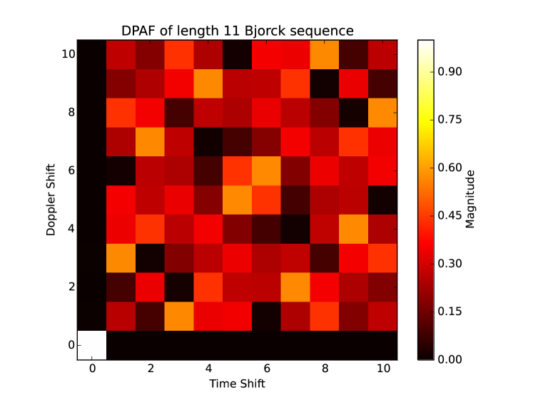
Figure 3.1. DPAF of length 11 Björck sequence.

Figure 3.1 shows that the length 11 Björck sequence is indeed a CAZAC sequence. In fact, all sequences generated by bjodef are CAZAC [10]. In this particular example, one can see that the discrete periodic ambiguity function of the length 11 Björck sequence is almost always nonzero, except for on $A_{p}(\varphi)[\cdot,0]$ and $A_{p}(\varphi)[0,\cdot]$. These properties hold true for any Björck sequence of any prime length. In light of aptightframe, we can see that Björck sequences are ill-suited to the construction of tight frames, despite being CAZAC. We shall explore this idea more in Section 5. More detailed exploration on the behavior of the DPAF of the Björck sequence can be found in [4] and [25]. For completeness, the length 11 Björck sequence is listed out below,

$$\varphi=(1,1,e^{i\theta_{11}},1,1,1,e^{i\theta_{11}},e^{i\theta_{11}},e^{i\theta_{11}},1,e^{i\theta_{11}}),$$

where $\theta_{11}=\text{arccos}(-10/11)$.

Proposition 3.6.

cazacprop Let $\varphi\in\mathbb{C}^{N}$ and let $c\in\mathbb{C}$ be such that $|c|=1$. Then,

• If $\varphi$ is CA, then $\widehat{\varphi}$ is ZAC.

• If $\varphi$ is CAZAC, then $\widehat{\varphi}$ is also CAZAC.

• If $\varphi$ is CA, then $\widehat{\varphi}$ can have zeros.

• If $\varphi$ is CAZAC, then $c\varphi$ is also CAZAC.

Property (iv) allows us to say two CAZACs are equivalent if they are complex rotations of each other. We can assume that the representative CAZAC in each equivalence class is the sequence whose first entry is 1. Given this, a natural question is as follows: For each $N$, how many CAZACs are there of length $N$? If $N$ is a prime number, then there are only finitely many classes of CAZAC sequences [23]. On the other hand, if $N$ is composite and is not square-free, then there are infinitely many classes of CAZAC sequences [11]. If $N$ is composite and square-free, it is unknown whether the number of equivalence classes is finite or infinite. Another question is, what other CAZACs can we construct besides the Chu, P4, etc.? The discovery of other CAZAC sequences can be transformed into two different problems in very different areas of mathematics. We shall explore these two other equivalent problems: The first involves circulant Hadamard matrices and the second is with cyclic n-roots.

Definition 3.7.

hadacircdef Let $H\in\mathbb{C}^{N\times N}$.

• $H$ is a Hadamard matrix if for every $(i,j)$, $|H_{i,j}|=1$ and $HH^{*}=NI\!d$.

• $H$ is a circulant matrix if for each $i$, the $i$-th row is a circular shift of the first row by $i-1$ entries to the right.

One can construct a circulant Hadamard matrix by making the first row a CAZAC sequence and each row after a shift of the previous row to the right. It is clear that this construction leads to a circulant matrix, and the ZAC property will guarantee that $HH^{*}=NI\!d$. Thus, given a CAZAC, we can generate a Hadamard matrix, and even better, we have the following theorem [9].

Theorem 3.8.

hadacirc $\varphi\in\mathbb{C}^{N\times N}$ if and only if the circulant matrix generated by $\varphi$ is a Hadamard matrix.

In particular, hadacirc gives a one-to-one correspondence between circulant $N\times N$ Hadamard matrices whose diagonal consists of ones and the equivalence classes of CAZAC sequences of length $N$. Therefore, an equiavlent problem to the discovery of additional CAZAC sequences is the computation of circulant Hadamard matrices. There is a significant amount of research and interest in Hadamard matrices, even outside of the context of CAZACs. A catalogue of complex Hadamard matrices with relevant citations can be found online at [12].

Definition 3.9.

$(z_{0},z_{1},\cdots,z_{N-1})\in\mathbb{C}^{N}$ is a cylclic N-root if it satisfies the following system of equations,

$$\begin{cases}z_{0}+z_{1}+\cdots+z_{N-1}=0\\ z_{0}z_{1}+z_{1}z_{2}+\cdots+z_{N-1}z_{0}=0\\ z_{0}z_{1}z_{2}+z_{1}z_{2}z_{3}+\cdots+z_{N-1}z_{0}z_{1}=0\\ \cdots\cdots\\ z_{0}z_{1}z_{2}\cdots z_{N-1}=1\end{cases}.$$ (3.2)

Let $\varphi\in\mathbb{C}^{N}$ be CAZAC with $\varphi[0]=1$. Let us emphasize the sequence nature of $\varphi\in\mathbb{C}^{N}$ and write $\varphi[k]=\varphi_{k}$. Then,

$$(z_{0},z_{1},\cdots,z_{N-1}):=\left(\frac{\varphi_{1}}{\varphi_{0}},\frac{\varphi_{2}}{\varphi_{1}},\cdots,\frac{\varphi_{0}}{\varphi_{N-1}}\right)$$ (3.3)

is a cylcic n-root. In fact, there is a one-to-one correspondence between cyclic n-roots and CAZAC sequences whose first entry is one [23]. In the same manner as circulant Hadamard matrices, finding cyclic N-roots is equivalent to finding CAZAC sequences of length $N$. In particular, using (3.3) we can see that we can construct CAZAC sequences by the following (recursive) formula:

$$\forall k\in\{1,2,\cdots,N-1\},\text{ }\varphi_{0}=1,\text{ }\varphi_{k}=\varphi_{k-1}z_{k-1}.$$ (3.4)

Cyclic $n$-roots can be used to show that the number of prime length CAZACs is finite. This was proved by Haagerup [23], but a summary, along with more results on CAZACs, can be found in [5].

It is still unclear what the exact role of CAZACs is in the generation of tight frames. Many of the known CAZAC sequences are suitable for generating tight Gabor frames, as we shall see in Section 5. On the other hand, the Björck sequence is also CAZAC but is very ill-suited for generating tight Gabor frames. Part of the difficulty is that although there are results quantifying the number of CAZAC sequences for given length $N$, very few of them have been explicitly written out. Many of the ones which are known are generated by roots of unity. The Björck sequence is the exception to this and is also the one that is ill-suited for generating tight Gabor frames. One could perhaps show that all CAZAC sequences generated by roots of unity (eg. Chu, P4, Wiener, roots of unity generated Milewski) will have sparse discrete periodic ambiguity functions. Hopefully, the eventual discovery of more CAZAC sequences will help further clarify the usability of CAZAC sequences to generate tight Gabor frames.

4. Discrete periodic ambiguity functions of selected sequences

The following two sections will be devoted to examples of aptightframe using the CAZAC sequences from Section 3 and various time-frequency subgroups. In this section we will compute the DPAFs for five classes of sequences: Chu, P4, Wiener, Square-length Björck-Saffari, and Milewski sequences.

4.1. Chu Sequence

The computation of the DPAF of the Chu sequence is as follows,

$$A_{p}(\varphi)[m,n]=\frac{1}{N}\sum_{k=0}^{N-1}e^{\pi i(k+m)(k+m-1)/N}e^{-\pi ik(k-1)/N}e^{-2\pi ink/N}=\frac{1}{N}\sum_{k=0}^{N-1}e^{\pi i[(k+m)(k+m-1)-k(k-1)-2nk]/N}$$

$$=\frac{1}{N}\sum_{k=0}^{N-1}e^{\pi i(k^{2}+2km+m^{2}-k-m-k^{2}+k-2nk)/N}=\frac{1}{N}\sum_{k=0}^{N-1}e^{\pi i(2km+m^{2}-m-2nk)/N}$$

$$=\frac{1}{N}e^{\pi i(m^{2}-m)/N}\sum_{k=0}^{N-1}e^{2\pi ik(m-n)/N}$$

$$=\begin{cases}e^{\pi i(m^{2}-m)/N},&\text{if }m\equiv n\mod N\\ 0,&\text{otherwise.}\end{cases}$$

Note that in particular, everything off of the line $n=m$ returns a zero. We will leverage this fact in several of the examples in Section 5.

4.2. P4 Sequence

The computation of the DPAF of the P4 sequence is as follows,

$$A_{p}(\varphi)[m,n]=\frac{1}{N}\sum_{k=0}^{N-1}e^{\pi i(k+m)(k+m-N)/N}e^{-\pi ik(k-N)/N}e^{-2\pi ink/N}$$

$$=\frac{1}{N}\sum_{k=0}^{N-1}e^{\pi i[(k+m)(k+m-N)-k(k-N)-2nk]/N}=\frac{1}{N}\sum_{k=0}^{N-1}e^{\pi i(k^{2}+2km+m^{2}-Nk-Nm-k^{2}+Nk-2nk)/N}$$

$$=\frac{1}{N}\sum_{k=0}^{N-1}e^{\pi i(m^{2}-Nm+2mk-2nk)/N}=\frac{1}{N}(-1)^{m}e^{\pi im^{2}/N}\sum_{k=0}^{N-1}e^{2\pi i(m-n)k/N}$$

$$=\begin{cases}(-1)^{m}e^{\pi im^{2}/N},&\text{if }m\equiv n\mod N\\ 0,&\text{otherwise.}\end{cases}$$

Like the Chu sequence, the DPAF of the P4 sequence is also only nonzero on the diagonal $n=m$. Due to this fact, the Chu and P4 sequences will be used interchangably in the examples.

4.3. Wiener Sequences

We start with the case where $N$ is odd. In this case, $\varphi$ has the form

$$\forall k\in(\mathbb{Z}/N\mathbb{Z}),\text{ }\varphi[k]=e^{2\pi isk^{2}/N}$$

Then, the computation of the DPAF is as follows,

$$A_{p}(\varphi)[m,n]=\frac{1}{N}\sum_{k=0}^{N-1}e^{2\pi is(k+m)^{2}/N}e^{-2\pi isk^{2}/N}e^{-2\pi ink/N}=\frac{1}{N}\sum_{k=0}^{N-1}e^{2\pi i(sk^{2}+2skm+sm^{2}-sk^{2}-nk)/N}$$

$$=\frac{1}{N}\sum_{k=0}^{N-1}e^{2\pi i(sm^{2}+2skm-nk)/N}=\frac{1}{N}e^{2\pi ism^{2}/N}\sum_{k=0}^{N-1}e^{2\pi i(2sm-n)k/N}$$

$$=\begin{cases}e^{2\pi ism^{2}/N},&\text{if }2sm\equiv n\mod N\\ 0,&\text{otherwise.}\end{cases}$$

The second case is where $N$ is even. In this case, $\varphi$ has the form

$$\varphi[k]=e^{\pi isk^{2}/N},\hskip 8.53581ptk\in\{0,\cdots,N-1\}.$$

In this case, the computation of the DPAF is as follows,

$$A_{p}(\varphi)[m,n]=\frac{1}{N}\sum_{k=0}^{N-1}e^{\pi is(k+m)^{2}/N}e^{-\pi isk^{2}/N}e^{-2\pi ink/N}=\frac{1}{N}\sum_{k=0}^{N-1}e^{\pi i(sk^{2}+2skm+sm^{2}-sk^{2}-2nk)/N}$$

$$=\frac{1}{N}\sum_{k=0}^{N-1}e^{\pi i(sm^{2}+2skm-2kn)/N}=e^{\pi ism^{2}/N}\frac{1}{N}\sum_{k=0}^{N-1}e^{2\pi i(sm-n)k/N}$$

$$=\begin{cases}e^{\pi ism^{2}/N},&\text{if }sm\equiv n\mod N\\ 0,&\text{otherwise.}\end{cases}$$

4.4. Square Length Björck-Saffari Sequences

The computation for the DPAF of the square length Björck-Saffari sequences is as follows,

$$A_{p}(\varphi)[sN+t,kN+\ell]=\frac{1}{N^{2}}\sum_{r=0}^{N-1}\sum_{h=0}^{N-1}\varphi[(r+s)N+(h+t)]\overline{\varphi[rN+h]}e^{-2\pi i(kN+\ell)(rN+h)/N^{2}}$$

$$=\frac{1}{N^{2}}\sum_{r=0}^{N-1}\sum_{h=0}^{N-1}c[h+t]\overline{c[h]}e^{2\pi i(r+s+\lfloor\frac{(h+t)}{N}\rfloor)\sigma(h+t)/N}e^{-2\pi ir\sigma(h)/N}e^{-2\pi i[(kh+r\ell)N+\ell h]/N^{2}}$$

$$=\frac{1}{N^{2}}\sum_{h=0}^{N-1}c[h+t]\overline{c[h]}e^{2\pi i(s+\lfloor\frac{(h+t)}{N}\rfloor)\sigma(h+t)/N}e^{-2\pi i(khN+\ell h)/N^{2}}\sum_{r=0}^{N-1}e^{2\pi i(\sigma(h+t)-\sigma(h)-\ell)r/N}$$

$$=\frac{1}{N}\sum_{h=0}^{N-1}c[h+t]\overline{c[h]}e^{2\pi i(s+\lfloor\frac{(h+t)}{N}\rfloor)\sigma(h+t)/N}e^{-2\pi i(khN+\ell h)/N^{2}}$$

if $\sigma(h+t)-\sigma(h)-\ell\equiv 0\mod N$, and 0 otherwise. In particular, if $\sigma(h)=h$ for all $h$, then the above condition reduces to $t\equiv\ell\mod N$.

4.5. Milewski sequences

We shall write out the DPAF of the Milewski sequence without computation, but the computation can be found in [6]. The DPAF of the Milewski sequence is,

$$NA_{p}(\varphi)[kN+\ell,s]=\begin{cases}0,&\text{ if }m\not\equiv n\mod N\\ \sum_{j=0}^{N-1}e^{2\pi i\left(k+\lfloor\frac{j+\ell}{N}\rfloor-js\right)/MN}A_{p}(v)\left[k+\lfloor\frac{j+\ell}{N}\rfloor,\frac{s-\ell}{N}\right],&\text{ if }m\equiv n\mod N.\\ \end{cases}$$ (4.1)

5. Examples of tight Gabor frames generated by $\Lambda^{\circ}$-sparsity

For the first examples, we will use the following subgroup $\Lambda\subseteq(\mathbb{Z}/N\mathbb{Z})\times(\mathbb{Z}/N\mathbb{Z})^{\widehat{}}$: Let $K=\{0,a,\cdots,(bN^{\prime}-1)a\}$ and $L=\{0,b,\cdots,(aN^{\prime}-1)b\}$ where $N=abN^{\prime}$ and gcd$(a,b)=1$ and let $\Lambda=K\times L$. We first shall compute the adjoint subgroup of $\Lambda=K\times L$. This requires us to compute which time-frequency translates $(m,n)$ commute with every time-frequency translate in $K\times L$. To that end, let $(k,\ell)$ and $(m,n)$ be two time-frequency translates. We compute,

$$(e_{n}\tau_{m}e_{\ell}\tau_{k})\varphi[j]=(e_{n}\tau_{m})(e^{2\pi i\ell j/N}\varphi[j-k])=e^{2\pi inj/N}e^{2\pi i\ell(j-m)/N}\varphi[j-k-m]$$

$$=e^{-2\pi i\ell m/N}(e_{\ell+n}\tau_{k+m})\varphi[j]$$

and

$$(e_{\ell}\tau_{k}e_{n}\tau_{m})\varphi[j]=(e_{\ell}\tau_{k})(e^{2\pi inj/N}\varphi[j-m])=e^{2\pi i\ell j/N}e^{2\pi in(j-k)/N}\varphi[j-k-m]$$

$$=e^{-2\pi ink/N}(e_{\ell+n}\tau_{k+m})\varphi[j].$$

Thus, $(m,n)\in\Lambda^{\circ}$ if and only if

$$\ell m\equiv kn\mod N,\hskip 14.22636pt\forall(k,\ell)\in\Lambda.$$ (5.1)

Since $k\in K$ and $\ell\in L$ we can write $k=k^{\prime}a$ and $\ell=\ell^{\prime}b$ for some $k^{\prime}\in\{0,\cdots,bN^{\prime}-1\}$ and $\ell^{\prime}\in\{0,\cdots,aN^{\prime}-1\}$. Using this in (5.1) gives a new condition

$$\ell^{\prime}bm\equiv k^{\prime}an\mod N,\forall(k^{\prime},\ell^{\prime})\in\{0,\cdots,bN^{\prime}-1\}\times\{0,\cdots,aN^{\prime}-1\}.$$ (5.2)

Lemma 5.1.

72sol Let $N=abN^{\prime}$ where gcd$(a,b)=1$. $(m,n)$ is a solution to (5.2) if and only if $m$ is a multiple of $N^{\prime}a$ and $n$ is a multiple of $N^{\prime}b$. In particular, if $\Lambda=K\times L$ where $K=\{0,a,\cdots,(bN^{\prime}-1)a\}$ and $L=\{0,b,\cdots,(aN^{\prime}-1)b\}$, then $\Lambda^{\circ}=N^{\prime}K\times N^{\prime}L=\{0,N^{\prime}a,\cdots,(b-1)N^{\prime}a\}\times\{0,N^{\prime}b,\cdots,(a-1)N^{\prime}b\}$.

Proof.

First note that if $m=rN^{\prime}a$ and $n=sN^{\prime}b$ for some $r\in\{0,\cdots,b-1\}$ and $s\in\{0,\cdots,a-1\}$ then the left hand side of (5.2) becomes

$$\ell^{\prime}b(rN^{\prime}a)\equiv\ell^{\prime}r(abN^{\prime})\equiv 0\mod N.$$ (5.3)

The right hand side of (5.2) becomes

$$k^{\prime}a(sN^{\prime}b)\equiv k^{\prime}s(abN^{\prime})\equiv 0\mod N.$$ (5.4)

Since (5.3) and (5.4) are equal we have that $N^{\prime}K\times N^{\prime}L\subseteq\Lambda^{\circ}$. To show the converse, first note that since gcd$(a,b)=1$, $m$ must be a multiple of $a$ and $n$ must be a multiple of $b$. In other words, $\Lambda^{\circ}\subseteq K\times L$. Now, suppose $m=ra$ and $n=sb$. Then, condition (5.2) becomes

$$\ell^{\prime}rab\equiv k^{\prime}sab\mod N,\forall(k^{\prime},\ell^{\prime})\in\{0,\cdots,bN^{\prime}-1\}\times\{0,\cdots,aN^{\prime}-1\}.$$ (5.5)

If $N^{\prime}=1$, the above is always true since $N=abN^{\prime}=ab$ and thus $\Lambda^{\circ}=N^{\prime}K\times N^{\prime}L=K\times L$. Assume that $N^{\prime}>1$ and without loss of generality, assume $N^{\prime}\nmid r$. Then, choose $\ell^{\prime}=1$ and $k^{\prime}=0$ and it is clear that the right hand side is 0 while the left hand side cannot be a multiple of $N$ and so (5.5) cannot hold. Thus, $N^{\prime}\mid r$ and $N^{\prime}\mid s$ is necessary and we now get $\Lambda^{\circ}\subseteq N^{\prime}K\times N^{\prime}L$ which completes the proof. $\blacksquare$

For our first example, we will use the $K\times L$ setup as above and apply it to the Chu and P4 sequence. As seen in Section 4.1 and Section 4.2, $A_{p}(\varphi)[m,n]$ only has nonzero entries along the diagonal $m=n$ and we will leverage this fact for an easy proof of chup4ap. It should also be noted that some slight modifications can be made to easily extend chup4ap to Wiener sequences.

Proposition 5.2.

chup4ap Let $\varphi\in\mathbb{C}^{N}$ be either the Chu or P4 sequence and let $K=\{0,a,\cdots,(bN^{\prime}-1)\}$ and $L=\{0,b,\cdots,(aN^{\prime}-1)b\}$ with gcd$(a,b)=1$ and $N=abN^{\prime}$. Then, the Gabor system $(\varphi,K\times L)$ is a tight Gabor frame with frame bound $NN^{\prime}$.

Proof.

Using 72sol we have that $(m,n)\in(K\times L)^{\circ}$ if and only if $m=raN^{\prime}$ and $n=sbN^{\prime}$ for some $r\in\{0,1,\cdots,bN^{\prime}-1\}$ and $s\in\{0,1,\cdots,aN^{\prime}-1\}$. However, $A_{p}(\varphi)[m,n]\neq 0$ if and only if $m\equiv n\mod N$. Thus, $A_{p}(\varphi)[m,n]\neq 0$ if and only if $m,n\in N^{\prime}K\cap N^{\prime}L$. This intersection is generated by lcm$(N^{\prime}a,N^{\prime}b)=N^{\prime}$ lcm$(a,b)=abN^{\prime}=N$. From this we conclude that for $(m,n)\in(K\times L)^{\circ}$, $A_{p}(\varphi)[m,n]\neq 0$ if and only if $m=n=0$. Thus by aptightframe, we have that $(\varphi,K\times L)$ is a tight frame with frame bound $|\Lambda|=NN^{\prime}$. $\blacksquare$

It should be noted that other subgroups $\Lambda\subseteq(\mathbb{Z}/N\mathbb{Z})\times(\mathbb{Z}/N\mathbb{Z})^{\widehat{}}$ can be used in chup4ap to get the same result. In this case, it is only necessary that for every $(m,n)\in\Lambda^{\circ}$, $m\not\equiv n\mod N$ unless $(m,n)=(0,0)$. We demonstrate this idea with chugenframe.

Proposition 5.3.

chugenframe Let $\varphi\in\mathbb{C}^{N}$ be either the Chu or P4 sequence and let $\Lambda=\{(0,0),(a,b),\\ (2a,2b),\cdots,((N-1)a,(N-1)b)\}$ where $a\neq b$ and gcd$(a,N)=$ gcd$(b,N)=1$. Then, the Gabor system $(\varphi,\Lambda)$ is a tight Gabor frame with frame bound $N$.

Proof.

Suppose gcd$(a,b)=d$. Let $a=da^{\prime}$ and $b=db^{\prime}$. Since gcd$(a,N)=1$ and gcd$(b,N)=1$, the order of the cyclic subgroup $\Lambda$ is $N$ and in particular is the same subgroup as the one generated by $(a^{\prime},b^{\prime})$. Thus, without loss of generality, we can assume that gcd$(a,b)=1$. Then, by (5.1), we know that $(m,n)\in\Lambda^{\circ}$ if and only if

$$kn\equiv\ell m\mod N$$

which can be rewritten as

$$san\equiv sbm\mod N.$$

Letting $s=1$, we see that $an\equiv bm\mod N$ is a necessary condition and since gcd$(a,b)=1$ we need that $n$ is a multiple of $b$ and $m$ is a multiple of $a$. It is clear that multiples of $(a,b)$ also work for $s\neq 1$ and so we have that $\Lambda^{\circ}=\Lambda$. Since gcd$(a,b)=1$, we have that $m=n$ if and only if $m=n=0$ and so $A_{p}(\varphi)[m,n]=0$ for every $(m,n)\in\Lambda^{\circ}$ except at $(0,0)$. Since $|\Lambda|=N$, we have that $(\varphi,\Lambda)$ is a tight frame with frame bound $N$. $\blacksquare$

The next example utilizes the square length Björck-Saffari sequence. From Section 4.4, the DPAF of the square length Björck-Saffari sequence is still very sparse, and the nonzero entries have regular structure as long as we take the identity permutation $\sigma(m)=m$. We leverage this fact to prove sqlenframe and apply the same techniques as in chup4ap.

Proposition 5.4.

sqlenframe Let $c\in\mathbb{C}^{N}$ and let $\varphi\in\mathbb{C}^{N^{2}}$ be the square length Björck-Saffari sequence generated by $c$ and $\sigma(h)=h$. Let $K=\{0,a,\cdots,(bN^{\prime}-1)a\}$ and $L=\{0,b,\cdots,(aN^{\prime}-1)b\}$ with gcd$(a,b)=1$ and $N^{2}=abN^{\prime}$. Then, the Gabor system $(\varphi,K\times L)$ is a tight Gabor frame with frame bound $N^{2}N^{\prime}$.

Proof.

Using 72sol, $\sigma(h)=h$, and the results of Section 4.4, if $(rN^{\prime}a,sN^{\prime}b)\in N^{\prime}K\times N^{\prime}L$, then $A_{p}(\varphi)[rN^{\prime}a,sN^{\prime}b]$ can only be nonzero if

$$rN^{\prime}a\equiv sN^{\prime}b\mod N$$ (5.6)

for some $r,s\in(\mathbb{Z}/N\mathbb{Z})$. From the proof of chup4ap, we know that $N^{\prime}K\cap N^{\prime}L$ is generated by lcm$(aN^{\prime},bN^{\prime})$. We have that lcm$(N^{\prime}a,N^{\prime}b)=N^{\prime}$ lcm$(a,b)=abN^{\prime}=N^{2}$, and we have that $N^{2}\equiv 0\mod N$. Moreover, if $A_{p}(\varphi)[rN^{\prime}a,sN^{\prime}b]\neq 0$, then $r=s=0$. Appealing once again to aptightframe, we have that $(\varphi,K\times L)$ is a tight Gabor frame, and the frame bound is $|\Lambda|=N^{2}N^{\prime}$. $\blacksquare$

We now give an example utilizing aptightframe, but with the opposite theme: the discrete periodic amibguity function will be mostly nonzero except for the “right” spots. That is, $A_{p}(\varphi)[m,n]\neq 0$ for nearly every $(m,n)\not\in\Lambda^{\circ}$ but $A_{p}(\varphi)$ will still be $\Lambda^{\circ}$-sparse.

Proposition 5.5.

Let $u\in\mathbb{C}^{M}$ be unimodular and satisfy

$$\forall k\in(\mathbb{Z}/N\mathbb{Z}),k\neq 0,\text{ }\langle\tau_{-k}u,u\rangle=NA_{p}(u)[k,0]=0.$$ (5.7)

Furthermore, let $v\in\mathbb{C}^{N}$ be also unimodular and let $\varphi\in\mathbb{C}^{MN}$ be defined by

$$\varphi=u\otimes v$$

where $\otimes$ is the Kronecker product. Assume gcd$(M,N)=1$ and let $\Lambda=\{0,M,\cdots,(N-1)M\}\times\{0,N,\cdots,(M-1)N\}$. Then, $(\varphi,\Lambda)$ is a tight frame with frame bound $MN$.

Proof.

We can write the $(rN+s)$-th term of $\varphi$ as

$$\varphi[rN+s]=u[r]v[s]$$

where $r\in(\mathbb{Z}/M\mathbb{Z})$ and $s\in(\mathbb{Z}/N\mathbb{Z})$. We now compute the DPAF,

$$A_{p}(\varphi)[rN+s,\ell]=\frac{1}{MN}\sum_{j=0}^{M-1}\sum_{k=0}^{N-1}u\left[j+r+\left\lfloor\frac{s+k}{N}\right\rfloor\right]v[s+k]\overline{u[j]v[k]}e^{-2\pi i(jN+k)\ell/MN}$$

$$=\frac{1}{N}\sum_{k=0}^{N-1}v[s+k]\overline{v[k]}e^{-2\pi ik\ell/MN}\frac{1}{M}\sum_{j=0}^{M-1}u\left[j+r+\left\lfloor\frac{s+k}{N}\right\rfloor\right]\overline{u[j]}e^{-2\pi ij\ell/M}$$

$$=\frac{1}{N}\sum_{k=0}^{N-1}v[s+k]\overline{v[k]}e^{-2\pi ik\ell/MN}A_{p}(u)\left[r+\left\lfloor\frac{s+k}{N}\right\rfloor,\ell\right].$$ (5.8)

By 72sol we have that $\Lambda^{\circ}=\Lambda$. Using (5.8), we can see that for $(rN,\ell M)\in\Lambda^{\circ}\setminus\{(0,0)\}$ we have

$$A_{p}(\varphi)[rN,\ell M]=\frac{1}{N}\sum_{k=0}^{N-1}v[k]\overline{v[k]}e^{-2\pi ik\ell/N}A_{p}(u)[r,\ell M]=\frac{A_{p}(u)[r,0]}{N}\sum_{k=0}^{N-1}|v[k]|^{2}e^{-2\pi ik\ell/N}=0$$

since one of $r$ or $\ell$ is nonzero. Indeed, if $r$ is nonzero, then by (5.7) we have a multiplier of zero outside of the sum and if $r=0$ but $\ell\neq 0$ then the sum will add up to zero since $|v[k]|^{2}=1$ for every $k$. We now conclude by aptightframe that $(\varphi,\Lambda)$ is a tight frame with frame bound $MN$. $\blacksquare$

Although $A_{p}(\varphi)$ is $\Lambda^{\circ}$-sparse, (5.8) implies that most of the entries for $A_{p}(\varphi)$ are nonzero. This is illustrated by Figure 5.1. In Figure 5.1, $u$ is the Björck sequence which is defined in Section 3. The definition of the Björck sequence and some of its relevant properties are defined in can also be found in [9]. It should be noted that the Björck sequence is not the same as the square length Björck-Saffari sequences defined in Section 4.

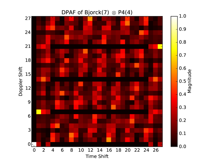
Figure 5.1. DPAF of $\varphi=u\otimes v$ where $u$ is the length 7 Björck sequence and $v$ is the length 4 P4 sequence.

Proposition 5.6.

Let $\varphi\in\mathbb{C}^{MN^{2}}$ be a Milewski sequence where the generating $v\in C^{M}$ is either the Chu or P4 sequence, and let $a,b,j,N^{\prime}$ be such that gcd$(a,b)=1$, $j\mid MN$, $N^{\prime}=jN$, and $abN^{\prime}=MN^{2}$. Let $\Lambda=K\times L$ where $K=\{0,a,\cdots,(bN^{\prime}-1)a\}$, and $L=\{0,b,\cdots,(aN^{\prime}-1)b\}$. Then, $(\varphi,\Lambda)$ is a tight frame with frame bound $jMN^{3}$.

Proof.

By 72sol, we have that $\Lambda^{\circ}=N^{\prime}K\times N^{\prime}L$. In particular, for every $(m,n)\in\Lambda^{\circ}$ we have that $m\equiv n\equiv 0\mod N$. Thus, using the second line of (4.1), for $(m,n)\in\Lambda^{\circ}$ we can write $A_{p}(\varphi)[m,n]$ in the form

$$NA_{p}(\varphi)[m,n]=\sum_{j=0}^{N-1}e^{\theta[j]}A_{p}(v)[m^{\prime},n^{\prime}]$$

where $m^{\prime}=m/N$ and $n^{\prime}=n/N$. Since $v$ is the Chu or P4 sequence, we have that $A_{p}(v)[m^{\prime},n^{\prime}]\neq 0$ if and only if $m^{\prime}\equiv n^{\prime}\mod M$. Furthermore, $\Lambda^{\circ}=\langle aN^{\prime}\rangle\times\langle bN^{\prime}\rangle=\langle ajN\rangle\times\langle bjN\rangle$ and so we have that $m^{\prime}\in\langle aj\rangle$ and $n^{\prime}\in\langle bj\rangle$. Thus, we have that $m^{\prime}\equiv n^{\prime}$ if and only if $m^{\prime},n^{\prime}\in\langle aj\rangle\cap\langle bj\rangle=\langle\text{lcm}(aj,bj)\rangle$. Since gcd$(a,b)=1$, we have that lcm$(aj,bj)=abj=MN$ since $abjN=abN^{\prime}=MN^{2}$. In particular, we want to view $\langle aj\rangle$ and $\langle bj\rangle$ as being subgroups of $(\mathbb{Z}/MN\mathbb{Z})$ and in light of this we have that $m^{\prime}\equiv n^{\prime}\mod MN$ if and only if $m^{\prime}\equiv n^{\prime}\equiv 0\mod MN$. Thus, we have that for $(m,n)\in\Lambda^{\circ}$, $A_{p}(\varphi)=0$ unless $(m,n)=(0,0)$. Using aptightframe, we finally conclude that $(\varphi,\Lambda)$ is a tight frame with frame bound $jMN^{3}$. $\blacksquare$

6. Gram matrices in terms of the discrete periodic ambiguity function

The last three sections are devoted to an alternative method for showing when Gabor systems are tight frames. The general framework is as follows: First, we explicitly compute the entries of the Gram matrix by using the discrete periodic ambiguity function. Then, we show that the first $N$ columns or rows happen to have disjoint supports. Last, we show that every other column or row is a constant multiple of one of the first $N$ rows or columns and use this to show that all $N$ nonzero eigenvalues are the same. This allows us to conclude that the Gabor system is indeed a tight frame. We begin by defining the frame operator and Gram operator and comparing the two.

6.1. Gram Operator and Frame Operator

Let $\mathcal{H}$ be an $N$-dimensional Hilbert space and let $\mathcal{F}=\{v_{i}\}_{i=1}^{M}\subseteq\mathcal{H}$ be a frame for $\mathcal{H}$, where $M\geq N$. We define the analysis operator $F:\mathcal{H}\to\mathbb{R}^{M}$ by

$$\forall x\in\mathcal{H},\text{ }F(x)=\{\langle x,v_{i}\rangle\}_{i=1}^{M}.$$ (6.1)

The adjoint of the analysis operator, $F^{*}:\mathbb{R}^{M}\to\mathcal{H}$, is called the synthesis operator and is given by

$$\forall\{c_{i}\}_{i=1}^{M}\in\mathbb{R}^{M},\text{ }F^{*}(\{c_{i}\}_{i=1}^{M})=\sum_{i=1}^{M}c_{i}v_{i}.$$ (6.2)

Given the analysis and the synthesis operator, we can now define the frame operator of the frame $\mathcal{F}$. The frame operator, $S:\mathcal{H}\to\mathcal{H}$, is defined by $S=F^{*}F$. We can write this explicitly as

$$\forall x\in\mathcal{H},\text{ }S(x)=\sum_{i=1}^{M}\langle x,v_{i}\rangle v_{i}.$$ (6.3)

Note that $S$ is a self-adjoint operator. Indeed, $S^{*}=(F^{*}F)^{*}=F^{*}F^{**}=F^{*}F=S$. We can define a second operator by reversing the order of the analysis and synthesis operator. That is, we apply the synthesis operator first and the analysis operator second. This new operator $G:\mathbb{R}^{M}\to\mathbb{R}^{M}$ is called the Gram operator and is defined by $G=FF^{*}$. We can write this explicitly as

$$\forall\{c_{i}\}_{i=1}^{M}\in\mathbb{R}^{M},\text{ }F(\{c_{i}\}_{i=1}^{M})=\left\{\left\langle\sum_{i=1}^{M}c_{i}v_{i},v_{j}\right\rangle\right\}_{j=1}^{M}.$$ (6.4)

(6.4) is unwieldy and so it is usually more convenient to write the Gram operator in matrix form. Once can see from (6.4) that we can write the $(i,j)$-th entry of the matrix form of $G$ as $G_{i,j}=\langle v_{i},v_{j}\rangle$. A detailed exposition on finite frames, the frame operator, and the Gram operator can be found in the first chapter of [15], but we will use the following fact in Section 7.

Theorem 6.1.

gramtightframes Let $\mathcal{H}$ be an $N$-dimensional Hilbert space and let $\mathcal{F}=\{v_{i}\}_{i=1}^{M}$ be a frame for $\mathcal{H}$. $\mathcal{F}$ is a tight frame if and only if rank$(G)=N$ and every nonzero eigenvalue of $G$ is equal.

6.2. Gram Matrix of Gabor Systems

In this section, we show that each entry of the Gram matrix of a Gabor system can be written in terms of the discrete periodic ambiguity function of the $\varphi\in\mathbb{C}^{N}\setminus\{0\}$ which generates the system. For all that follows let $\varphi\in\mathbb{C}^{N}\setminus\{0\}$ and let us write out the Gabor system as $\mathcal{F}=\{e_{\ell_{m}}\tau_{k_{m}}\varphi:m\in{0,\cdots,M}\}$. Then, we can compute the $(m,n)$-th entry of the Gram matrix:

$$G_{m,n}=\langle e_{\ell_{m}}\tau_{k_{m}}\varphi,\overline{e_{\ell_{n}}\tau_{k_{n}}\varphi}\rangle=\sum_{j=0}^{N}e^{2\pi i\ell_{m}j/N}\varphi[j-k_{m}]e^{-2\pi i\ell_{n}j/N}\overline{\varphi[j-k_{n}]}$$

$$=\sum_{j=0}^{N}e^{-2\pi i(\ell_{n}-\ell_{m})j/N}\varphi[j-k_{m}]\overline{\varphi[j-k_{n}]}=\sum_{j=0}^{N}e^{-2\pi i(\ell_{n}-\ell_{m})(j-k_{n}+k_{n})/N}\varphi[j-k_{n}+(k_{n}-k_{m})]\overline{\varphi[j-k_{n}]}$$

$$=e^{-2\pi ik_{n}(\ell_{n}-\ell_{m})/N}\sum_{j=0}^{N}\varphi[j+(k_{n}-k_{m})]\overline{\varphi[j]}e^{-2\pi i(\ell_{n}-\ell_{m})j/N}=Ne^{-2\pi ik_{n}(\ell_{n}-\ell_{m})/N}A_{p}(\varphi)[k_{n}-k_{m},\ell_{n}-\ell_{m}]$$

6.3. Gram Matrix for Chu Sequences

In the Chu sequence case, we have that $G_{m,n}\neq 0$ if and only if $(\ell_{n}-\ell_{m})\equiv(k_{n}-k_{m})\mod N$. For convenience, let us define $r_{mn}:\equiv k_{n}-k_{m}\equiv\ell_{n}-\ell_{m}\mod N$. Then, the Gram matrix for the Chu sequence is,

$$G_{mn}=\begin{cases}Ne^{-2\pi i[k_{n}r_{mn}-\frac{1}{2}(r_{mn}^{2}-r_{mn})]/N},&\text{if }(\ell_{n}-\ell_{m})\equiv(k_{n}-k_{m})\mod N\\ 0,&\text{otherwise.}\end{cases}$$ (6.5)

6.4. Gram Matrices for P4 Sequences

In the P4 sequence case, we also have that $G_{m,n}\neq 0$ if and only if $(\ell_{n}-\ell_{m})\equiv(k_{n}-k_{m})\mod N$. Again, let $r_{mn}:\equiv k_{n}-k_{m}\equiv\ell_{n}-\ell_{m}\mod N$. Then, the Gram matrix for the P4 sequence is,

$$G_{mn}=\begin{cases}N(-1)^{r_{mn}}e^{-2\pi i[k_{n}r_{mn}-\frac{1}{2}r_{mn}^{2}]/N},&\text{if }(k_{n}-k_{m})\equiv(\ell_{n}-\ell_{m})\mod N\\ 0,&\text{otherwise.}\end{cases}$$ (6.6)

6.5. Gram Matrices for Wiener Sequences

In the Wiener sequence case, we have the following formula for the Gram matrices. If $N$ is odd, then $G_{mn}\neq 0$ if and only if $2s(k_{n}-k_{m})\equiv(\ell_{n}-\ell_{m})\mod N$. Let $r_{mn}:\equiv(k_{n}-k_{m})\mod N$. Then we can write $G_{mn}$ as

$$G_{mn}=\begin{cases}Ne^{-4\pi isk_{n}r_{mn}/N}e^{2\pi isr_{mn}^{2}/N},&\text{ if }2s(k_{n}-k_{m})\equiv(\ell_{n}-\ell_{m})\mod N\\ 0,&\text{ otherwise.}\\ \end{cases}$$

If $N$ is even, then then $G_{mn}\neq 0$ if and only if $s(k_{n}-k_{m})\equiv(\ell_{n}-\ell_{m})\mod N$. Let $r_{mn}:\equiv(k_{n}-k_{m})\mod N$. Then we can write $G_{mn}$ as

$$G_{mn}=\begin{cases}Ne^{-2\pi isk_{n}r_{mn}/N}e^{\pi ism^{2}/N},&\text{ if }s(k_{n}-k_{m})\equiv(\ell_{n}-\ell_{m})\mod N\\ 0,&\text{ otherwise.}\\ \end{cases}$$

7. Gram matrix method

In this section, we begin by applying the method outlined in Section 6 and apply it to the Chu and P4 sequence. We treat these two cases simultaneously since both have the property that $A_{p}(\varphi)[m,n]=0$ if $m\neq n$, and are nonzero when $m=n$. The computation in chufnc will be different for the P4 case, but the same ideas can be applied to do the computation in the P4 case and achieve the same result. In the last part of this section we briefly discuss the Wiener sequence case. The Wiener case has direct analogues of the results in the Chu and P4 cases and we will only highlight the key differences in the proofs rather than reiterate all of the details. Before proceeding, we will need a useful fact about the Gram matrix which can easily be derived from the singular value decomposition of the analysis operator.

Lemma 7.1.

svdrank Let $F$ be an $m\times n$ complex-valued matrix and let $G:=FF^{*}$. Then, rank($G$) = rank($F$).

Proof.

First, we write $F$ in terms of its SVD: $F=UDV^{*}$ where $D$ is an $m\times n$ rectangular diagonal matrix and $U$ and $V$ are $m\times m$ and $n\times n$ unitary matrices, respectively. Note that $G=FF^{*}=UDV^{*}VD^{*}U^{*}=UDD^{*}U^{*}=UD^{2}U^{*}$. In particular, $D^{2}_{ij}=|D_{ij}|^{2}$ and from this we get that $\text{rank}(G)=\text{rank}(F)$. $\blacksquare$

For the following propostions, we shall use the following arrangement for the Gram matrix. Let $(\varphi,K\times L)$ be a Gabor system in $\mathbb{C}^{N}$. We shall iterate first by modulation, then iterate through translations. In other words, the analysis operator, $F$, will be a $|K||L|\times N$ matrix where the $m$-th row is given by $m=r|L|+s$, where $r\in\{0,\cdots,|K|-1\}$, $s=\{0,\cdots,|L|-1\}$, and the $m=r|L|+s$-th row corresponds to $e_{\ell_{s}}\tau_{k_{r}}\varphi$.

Proposition 7.2.

abframe Let $N=ab$ with gcd$(a,b)=1$ and let $\varphi\in\mathbb{C}^{N}$ be either the Chu or P4 sequence. Let $K=\{0,a,\cdots,(b-1)a\}$ and $L=\{0,b,\cdots,(a-1)b\}$. Then, the Gabor system $(\varphi,K\times L)$ is a tight frame with frame bound $N$.

Proof.

By construction, $|K|=b$, $|L|=a$ and so the Gabor system $(\varphi,K\times L)$ has $ab=N$ vectors. Since lcm$(a,b)=N$, we have that $K\cap L=\{0\}$. From Section 6.3, we have that $G_{m,n}\neq 0$ if and only if $(\ell_{n}-\ell_{m})=(k_{n}-k_{m})$. However, by design of $K$ and $L$, we have that $(\ell_{n}-\ell_{m})=jb$ and $(k_{n}-k_{m})=\tilde{j}a$ for some $j,\tilde{j}$. In particular, $(k_{n}-k_{m})\in K$ and $(\ell_{n}-\ell_{m})\in L$, and thus they are only equal if they both belong to $K\cap L$. From this we conclude that $G_{m,n}\neq 0$ if and only if $(\ell_{n}-\ell_{m})=(k_{n}-k_{m})=0$, i.e. $j=\tilde{j}=0$. We conclude that the nonzero entries lie only on the diagonal of $G$. Using formulas (6.5) and (6.6), we see that for each $n\in\{0,\cdots,N-1\}$, $G_{n,n}=N$ and $G=NI\!d_{N}$. Thus, the Gabor system $(\varphi,K\times L)$ is a tight frame with frame bound $N$. $\blacksquare$

Lemma 7.3.

chufnc Let $\varphi\in\mathbb{C}^{N}$ be either the Chu or P4 sequence and let $N=abN^{\prime}$ where gcd$(a,b)=1$. Suppose $G$ is the Gram matrix generated by the Gabor system $(\varphi,K\times L)$ where $K=\{0,a,\cdots,(bN^{\prime}-1)a\}$ and $L=\{0,b,\cdots,(aN^{\prime}-1)b\}$. Then, there exist functions $f,g:\mathbb{N}\cup\{0\}\to\mathbb{C}$ such that $G_{mn}/N=f(n)g(m)$ wherever $G_{mn}\neq 0$.

Proof.

We will only cover the case of the Chu sequence. The case of the P4 sequence follows by replacing $e^{-\pi ir_{mn}/N}$ with $(-1)^{r_{mn}}$ and carrying out the same computations. If $G_{mn}\neq 0$, then we have

$$G_{mn}/N=e^{-2\pi ik_{n}r_{mn}/N}e^{-\pi ir_{mn}/N}e^{\pi ir_{mn}^{2}/N}$$ (7.1)

where

$$r_{mn}=k_{n}-k_{m}=\ell_{n}-\ell_{m}=jab.$$ (7.2)

Note that $k_{n}=c_{n}ab+d_{n}a$ and $k_{m}=c_{m}ab+d_{m}a$ where $c_{n},c_{m}\in\{0,\cdots,N^{\prime}-1\},d_{n},d_{m}\in\{0,\cdots,b-1\}$. However, by (7.2), $j=c_{n}-c_{m}$ and $d_{n}=d_{m}$. Putting this back into (7.1) we have

$$G_{mn}/N=e^{-2\pi i(c_{n}ab+d_{n}a)(c_{n}-c_{m})ab/N}e^{-\pi i(c_{n}-c_{m})ab/N}e^{\pi i(c_{n}-c_{m})^{2}a^{2}b^{2}/N}$$

$$=e^{-2\pi ic_{n}ab(c_{n}-c_{m})/N^{\prime}}e^{-2\pi id_{n}a(c_{n}-c_{m})/N^{\prime}}e^{-\pi i(c_{n}-c_{m})/N^{\prime}}e^{\pi iab(c_{n}^{2}-2c_{n}c_{m}+c_{m}^{2})/N^{\prime}}$$

$$=e^{-2\pi ic_{n}^{2}ab/N^{\prime}}e^{2\pi ic_{n}c_{m}ab/N^{\prime}}e^{-2\pi id_{n}a(c_{n}-c_{m})/N^{\prime}}e^{-\pi i(c_{n}-c_{m})/N^{\prime}}e^{\pi iab(c_{n}^{2}+c_{m}^{2})/N^{\prime}}e^{-2\pi iabc_{n}c_{m}/N^{\prime}}$$

$$=e^{-\pi ic_{n}^{2}ab/N^{\prime}}e^{-2\pi id_{n}c_{n}a/N^{\prime}}e^{-\pi ic_{n}/N^{\prime}}e^{\pi ic_{m}^{2}ab/N^{\prime}}e^{2\pi id_{m}c_{m}a/N^{\prime}}e^{\pi ic_{m}/N^{\prime}}.$$

Here we have used the crucial fact that $d_{n}=d_{m}$. Thus, we can write nonzero entries of $G_{mn}$ as $f(n)g(m)$ where

$$f(n)=e^{-\pi ic_{n}^{2}ab/N^{\prime}}e^{-2\pi id_{n}c_{n}a/N^{\prime}}e^{-\pi ic_{n}/N^{\prime}}$$

and

$$g(m)=e^{\pi ic_{m}^{2}ab/N^{\prime}}e^{2\pi id_{m}c_{m}a/N^{\prime}}e^{\pi ic_{m}/N^{\prime}}.\blacksquare$$

Lemma 7.4.

chudisj Let $\varphi\in\mathbb{C}^{N}$ be either the Chu or P4 sequence and let $N=abN^{\prime}$ where gcd$(a,b)=1$. Suppose $G$ is the Gram matrix generated by the Gabor system $(\varphi,K\times L)$ where $K=\{0,a,\cdots,(bN^{\prime}-1)a\}$ and $L=\{0,b,\cdots,(aN^{\prime}-1)b\}$. Then, the support of the rows (or columns) of $G$ either completely coincide or are completely disjoint.

Proof.

Let us denote the $m$-th row of $G$ as $g_{m}$, and all indices are implictly taken modulo $N$. We shall show that if there is at least one index $n\in(\mathbb{Z}/N\mathbb{Z})$ such that $g_{m}[n]=g_{m^{\prime}}[n]\neq 0$, and $m\neq m^{\prime}$, then supp$(g_{m})=$ supp$(g_{m^{\prime}})$. Suppose that $g_{m}[n]=g_{m^{\prime}}[n]\neq 0$. Then, $k_{n}-k_{m}=\ell_{n}-\ell_{m}=jab$ and $k_{n}-k_{m^{\prime}}=\ell_{n}-\ell_{m^{\prime}}=j^{\prime}ab$. We can rearrange these two equations to obtain the following

$$k_{m}=k_{n}-jab$$ (7.3)

and

$$k_{n}=k_{m^{\prime}}+j^{\prime}ab.$$ (7.4)

Now suppose there is another $n^{\prime}\in(\mathbb{Z}/N\mathbb{Z})$ where $g_{m}[n^{\prime}]\neq 0$. Then, we have

$$k_{n^{\prime}}-k_{m}=\tilde{j}ab.$$ (7.5)

Substiuting (7.3) and (7.4) into (7.5), we have

$$\tilde{j}ab=k_{n^{\prime}}-k_{m}=k_{n^{\prime}}-k_{n}+jab=k_{n^{\prime}}-k_{m^{\prime}}-j^{\prime}ab+jab,$$

which can be rearranged to obtain

$$(j^{\prime}+\tilde{j}-j)ab=k_{n^{\prime}}-k_{m^{\prime}}.$$

Note that $(j^{\prime}+\tilde{j}-j)\in(\mathbb{Z}/N\mathbb{Z})$ and that these same computations can be done replacing $k$ with $\ell$. Thus, $g_{m^{\prime}}[n^{\prime}]\neq 0$ as well and the result is proved. $\blacksquare$

Remark 7.5.

Let gcd$(a,b)=1$, $N=abN^{\prime}$, $K=\{0,a,\cdots,(bN^{\prime}-1)a\}$, $L=\{0,b,\cdots,(aN^{\prime}-1)b\}$, $\varphi\in\mathbb{C}^{N}$ be the Chu and P4 sequence, and consider the system $(\varphi,K\times L)$. In light of chufnc and chudisj, if two rows of the Gram matrix $G$ have supports which coincide, they must be constant multiples of each other which has modulus 1. Indeed, if $g_{m}$ and $g_{m^{\prime}}$ have coinciding supports then for each $n$ where they are nonzero we have

$$\frac{G_{mn}}{G_{m^{\prime}n}}=\frac{Nf(n)g(m)}{Nf(n)g(m^{\prime})}=\frac{g(m)}{g(m^{\prime})}$$

which also gives us a formula for finding the constant multiple, should we desire it. This idea is illustrated with Figure 7.1, where two sets of rows with coinciding supports are highlighted in red and blue, respectively.

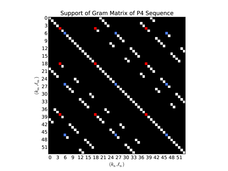
Figure 7.1. Support of $G$ in the case $N$ = 18, $\varphi$ is the P4 sequence, $a=2$, $b=3$, and $N^{\prime}=3$.

Theorem 7.6.

chuframe Let $K=\{0,a,\cdots,(b-1)a\}$, $L=\{0,b,\cdots,(a-1)b\}$, and $N=abN^{\prime}$ with gcd$(a,b)=1$. Furthermore, let $\varphi\in\mathbb{C}^{N}$ be either the Chu or P4 sequence. Then, the Gabor system $(\varphi,K\times L)$ has the following properties:

• rank$(G)=N$.

• The nonzero eigenvalues of $G$ are $NN^{\prime}$.

In particular, (i) and (ii) together imply that the Gabor system $(\varphi,K\times L)$ is a tight frame with frame bound $NN^{\prime}$.

Proof.

(i) We shall show that the first $N$ columns are disjoint, and then conclude that rank$(G)=N$. Note that $K$ and $L$ are subgroups of $(\mathbb{Z}/N\mathbb{Z})$ and that $K\cap L=\{0,ab,2ab,\cdots,(N^{\prime}-1)ab\}$. Moreover, $G_{mn}\neq 0$ if and only if $(\ell_{n}-\ell_{m})\equiv(k_{n}-k_{m})\mod N$. Since $K$ and $L$ are subgroups, this can only happen if the subtractions lie in the intersections of the two groups. That is, $G_{mn}\neq 0$ if and only if

$$(\ell_{n}-\ell_{m})\equiv(k_{n}-k_{m})\equiv jab\mod N$$ (7.6)

where $j\in\{0,\cdots,N^{\prime}-1\}$. Let $m\in(\mathbb{Z}/N\mathbb{Z})$. By $(\ref{condi})$, we have that for $G_{mn}\neq 0$ we must have that $k_{n}=(k_{m}+jab)$ for some $j$. Since $k_{m}\in K$, we have that

$$k_{n}=(j_{m}a+jab)=a(j_{m}+jb)$$ (7.7)

for some $j_{m}\in\{0,\cdots,bN^{\prime}-1\}$ and some $j\in\{0,\cdots,N^{\prime}-1\}$.

By the ordering we used for the columns of $G$, we can write the index for column $n$ in terms of $k_{n}$ and $\ell_{n}$ by

$$n=(k_{n}/a)aN^{\prime}+\ell_{n}/b=k_{n}N^{\prime}+\ell_{n}/b.$$ (7.8)

In particular, we would like $n\leq N$, and for that we need that $k_{n}<ab$. Looking at (7.7), we need $(j_{m}+jb)<b$. There is exactly 1 such $j\in\{0,\cdots N^{\prime}-1\}$ which can achieve this and it is obtained by setting $j=-\lfloor{j_{m}/b}\rfloor$. Thus, for each row $m$, there is exactly 1 column $n\leq N$ where $G_{mn}\neq 0$, and therefore the first $N$ columns of $G$ are linearly independent. Thus, we conclude $\text{rank}(G)\geq N$. By svdrank, we know that rank($G$) = rank($L$). Since $L$ is an $M\times N$ matrix, we have that $\text{rank}(G)\leq N$ and we have that $\text{rank}(G)=N$. We finally conclude the Gabor system in question forms a frame.

(ii) Let $g_{n}$ be the $n$-th column of $G$, with $n\leq N$. We wish to show that $Gg_{n}=NN^{\prime}g_{n}$. Note that $Gg_{n}[m]$ is given by the inner product of the $m$-th row and the $n$-th column of $G$. Furthermore, since $G$ is self-adjoint, the $n$-th column is also the conjugate of the $n$-th row. If $g_{n}[m]\neq 0$, then $G_{mn}\neq 0$ and $G_{nn}\neq 0$. Thus, by chudisj rows $m$ and $n$ have supports that coincide. By chufnc, $G_{m(\cdot)}=C_{m}g_{n}^{*}$, where $|C_{m}|=1$. Thus, $Gg_{n}[m]=C_{m}\|g_{n}\|_{2}^{2}=N^{2}N^{\prime}C_{m}$. It is easily computed that $G_{nn}=N$, so by chufnc, we have that $g_{n}[m]=NC_{m}$. In particular, we get $Gg_{n}[m]=(NN^{\prime})(NC_{m})$. Thus, the first $N$ columns of $G$ are eigenvectors of $G$ and they all have eigenvalue $NN^{\prime}$. It now follows that the system is a tight frame with frame bound $NN^{\prime}$. $\blacksquare$

Remark 7.7.

In general, if $\gcd(a,b)>1$, then the above result will not hold. Let $\varphi\in\mathbb{C}^{4}$ be the P4 sequence. That is, $\varphi=(1,-\sqrt{2}/2-i\sqrt{2}/2,-1,-\sqrt{2}/2-i\sqrt{2}/2)$. Let $K=\{0,2\}$ and $L=\{0,2\}$. Note that this would give $a=b=\gcd(a,b)=2$. The Gabor system $(\varphi,K\times L)$ is given by

$$(\varphi,K\times L)=\{\pi(0,0)\varphi,\pi(0,2)\varphi,\pi(2,0)\varphi,\pi(2,2)\varphi\}$$

$$=\left\{\begin{pmatrix}1\\ -\frac{\sqrt{2}}{2}-\frac{\sqrt{2}}{2}i\\ -1\\ -\frac{\sqrt{2}}{2}-\frac{\sqrt{2}}{2}i\end{pmatrix},\begin{pmatrix}1\\ \frac{\sqrt{2}}{2}+\frac{\sqrt{2}}{2}i\\ -1\\ \frac{\sqrt{2}}{2}+\frac{\sqrt{2}}{2}i\end{pmatrix},\begin{pmatrix}-1\\ -\frac{\sqrt{2}}{2}-\frac{\sqrt{2}}{2}i\\ 1\\ -\frac{\sqrt{2}}{2}-\frac{\sqrt{2}}{2}i\end{pmatrix},\begin{pmatrix}-1\\ \frac{\sqrt{2}}{2}+\frac{\sqrt{2}}{2}i\\ 1\\ \frac{\sqrt{2}}{2}+\frac{\sqrt{2}}{2}i\end{pmatrix},\right\}.$$

Note that the first and fourth vectors are multiples of each other, as well as the second and third vectors. Specifically,

$$\pi(0,0)\varphi=-\pi(2,2)\varphi\hskip 14.22636pt\text{ and }\hskip 14.22636pt\pi(0,2)\varphi=-\pi(2,0)\varphi.$$

We conclude from this that the dimension of the span of the Gabor system $(\varphi,K\times L)$ is only 2, and the Gabor system in question is not a frame.

We close this section with brief mentions about the proofs in the Wiener sequence case. To simplify further, we only mention the odd length case, but one can easily make the highlighted adjustments in the even case as well. The emphasis here is that the results and proofs in the Wiener cases are essentially the same.

Lemma 7.8.

wienerfnc Let $\varphi\in\mathbb{C}^{N}$ be a Wiener sequence of odd length and let $N=abN^{\prime}$ where gcd$(a,b)=1$. Suppose $G$ is the Gram matrix generated by the Gabor system $(\varphi,K\times L)$, where $K=\{0,a,\cdots,(bN^{\prime}-1)a\}$ and $L=\{0,b,\cdots,(aN^{\prime}-1)b\}$. Then, there exist functions $f,g:\mathbb{N}\cup\{0\}\to\mathbb{C}$ such that $G_{mn}/N=f(n)g(m)$ wherever $G_{mn}\neq 0$.

To prove wienerfnc, the same technique used in chufnc of writing $k_{n}=c_{n}ab+d_{n}a$ and $k_{m}=c_{m}ab+d_{m}a$ works here as well and the result follows from the same type of computations used in chufnc.

Lemma 7.9.

wienerdisj Let $\varphi\in\mathbb{C}^{N}$ be a Wiener sequence of odd length and let $N=abN^{\prime}$ where gcd$(a,b)=1$. Suppose $G$ is the Gram matrix generated by $(\varphi,K\times L)$, where $K=\{0,a,\cdots,(bN^{\prime}-1)a\}$ and $L=\{0,b,\cdots,(aN^{\prime}-a)b\}$. Then, the support of the rows (and columns) of $G$ either completely coincide or are completely disjoint.

To prove wienerdisj, one needs to replace $jab$, $j^{\prime}ab$, $\tilde{j}ab$ in chudisj with $2sjab$, $2sj^{\prime}ab$, and $2s\tilde{j}ab$, and the same result will hold.

Theorem 7.10.

wienerframe Let $K=\{0,a,\cdots,(b-1)a\}$, $L=\{0,b,\cdots,(a-1)b\}$, and $N=abN^{\prime}$ with gcd$(a,b)=1$. Furthermore, let $\varphi\in\mathbb{C}^{N}$ be a Wiener sequence of odd length. Then, the Gabor system $(\varphi,K\times L)$ has the following properties:

• rank$(G)=N$.

• The nonzero eigenvalues of $G$ are $NN^{\prime}$.

In particular, (i) and (ii) combined imply that the Gabor system $(\varphi,K\times L)$ is a tight frame with bound $NN^{\prime}$.

As with the modification used in wienerdisj, one only needs to change any instance of $jab$ in chuframe with $2sjab$ and apply the appropriate computations to prove wienerframe.

References

- [1] Radu Balan, Peter G. Casazza, Christopher Heil, and Zeph Landau. Density, overcompleteness, and localization of frames. I. Theory. Journal of Fourier Analysis and Applications, 12(2):105–143, 2006.
- [2] Radu Balan, Peter G. Casazza, Christopher Heil, and Zeph Landau. Density, overcompleteness, and localization of frames. II. Gabor systems. Journal of Fourier Analysis and Applications, 12(3):307–344, 2006.
- [3] John J. Benedetto. Frame decompositions, sampling, and uncertainty principle inequalities. In Wavelets: Mathematics and Applications, chapter 7, pages 247–304. CRC Press, 1993.
- [4] John J. Benedetto, Robert L. Benedetto, and Joseph T. Woodworth. Optimal ambiguity functions and Weil’s exponential sum bound. Journal of Fourier Analysis and Applications, 18(3):471–487, 2012.
- [5] John J. Benedetto, Katherine Cordwell, and Mark Magsino. CAZAC sequences and Haagerup’s characterization of cyclic n-roots. pre-print.
- [6] John J. Benedetto and Jeffrey J. Donatelli. Ambiguity function and frame-theoretic properties of periodic zero-autocorrelation waveforms. IEEE Journal of Selected Topics in Signal Processing, 1(1):6–20, 2007.
- [7] John J. Benedetto and Matthew Fickus. Finite normalized tight frames. Advances in Computational Mathematics, 18(2-4):357–385, 2003.
- [8] John J. Benedetto, Christopher Heil, and David F. Walnut. Gabor systems and the Balian-Low theorem. In Gabor Analysis and Algorithms, pages 85–122. Springer, 1998.
- [9] John J. Benedetto, Ioannis Konstantinidis, and Muralidhar Rangaswamy. Phase-coded waveforms and their design. IEEE Signal Processing Magazine, 26(1):22–33, 2009.
- [10] Göran Björck. Functions of modulus 1 on whose Fourier transforms have constant modulus and “cyclic -roots”. In Recent Advances in Fourier Analysis and its Applications, pages 131–140. Springer, 1990.
- [11] Göran Björck and Bahman Saffari. New classes of finite unimodular sequences with unimodular Fourier transforms. Circulant Hadamard matrices with complex entries. Comptes Rendus de l’Académie des Sciences. Série 1, Mathématique, 320(3):319–324, 1995.
- [12] Wojciech Bruzda, Wojciech Tadej, and Karol Życzkowski. Complex Hadamard matrices–a catalogue. http://chaos.if.uj.edu.pl/ karol/hadamard/?q=catalogue.
- [13] Peter G. Casazza and Jelena Kovačević. Equal-norm tight frames with erasures. Advances in Computational Mathematics, 18(2-4):387–430, 2003.
- [14] Peter G. Casazza and Gitta Kutyniok, editors. Finite Frames: Theory and Applications. Birkhäuser Basel, 2013.
- [15] Ole Christensen. Frames and Bases: An Introductory Course. Springer Science & Business Media, 2008.
- [16] Ingrid Daubechies. The wavelet transform, time-frequency localization and signal analysis. IEEE Transactions on Information Theory, 36(5):961–1005, 1990.
- [17] Ingrid Daubechies. Ten Lecutres on Wavelets, volume 61. SIAM, 1992.
- [18] Ingrid Daubechies, Bin Han, Amos Ron, and Zuowei Shen. Framelets: MRA-based constructions of wavelet frames. Applied and Computational Harmonic Analysis, 14(1):1–46, 2003.
- [19] Richard J. Duffin and Albert C. Schaeffer. A class of nonharmonic Fourier series. Transactions of the American Mathematics Society, 72(2):341–366, 1952.
- [20] Gerald Folland and Alladi Sitaram. The uncertainty principle: a mathematical survey. Journal of Fourier Analysis and Applications, 3(3):207–238, 1997.
- [21] Dennis Gabor. Theory of communication. part 1: Analysis of information. Electrical Engineers-Part III: Radio and Communiation Engineering, Journal of the Institution of, 93(26):429–441, 1946.
- [22] Karlheinz Gröchenig. Foundations of Time-Frequency Analysis. Springer Science & Business Media, 2013.
- [23] Uffe Haagerup. Cyclic p-roots of prime lengths and complex Hadamard matrices. arXiv preprint arXiv:0803.2629, 2008.
- [24] A.J.E.M. Janssen. Gabor representation of generalized functions. Journal of Mathematical Analysis and Applications, 83(2):377–394, 1981.
- [25] Andrew Kebo, Ioannis Konstantinidis, John J. Benedetto, Michael R. Dellomo, and Jeffrey M. Sieracki. Ambiguity and sidelobe behavior of CAZAC coded waveforms. In 2007 IEEE Radar Conference, pages 99–103. IEEE, 2007.
- [26] Jelena Kovačević and Amina Chebira. Life beyond bases: The advent of frames. IEEE Signal Processing Magazine, 2007.
- [27] Jelena Kovačević and Amina Chebira. Life beyond bases: The advent of frames (part ii). IEEE Signal Processing Magazine, 5(24):115–125, 2007.
- [28] Gitta Kutyniok, Kasso A. Okoudjou, Friedrich Philipp, and Elizabeth K. Tuley. Scalable frames. Linear Algebra and its Applications, 438(5):2225–2238, 2013.
- [29] Jim Lawrence, Götz Pfander, and David Walnut. Linear independence of Gabor systems in finite dimensional vector spaces. Journal of Fourier Analysis and Applications, 11(6):715–726, 2005.
- [30] Nadav Levanon and Eli Mozeson. Radar Signals. John Wiley & Sons, 2004.
- [31] Yurii Lyubarskii. Frames in the Bargmann space of entire functions. Entire and Subharmonic Functions, 11:167–180, 1992.
- [32] Stéphane Mallat. A Wavelet Tour of Signal Processing. Academic press, 1999.
- [33] Andrzej Milewski. Periodic sequences with optimal properties for channel estimation and fast start-up equalization. IBM Journal of Research and Development, 27(5):426–431, 1983.
- [34] Dustin Mixon. Sparse signal processing with frame theory. arXiv preprint arXiv:1204.5958, 2012.
- [35] Götz Pfander. Gabor frames in finite dimensions. In Finite Frames, pages 193–239. Springer, 2013.
- [36] Götz Pfander and Holger Rauhut. Sparsity in time-frequency representations. Journal of Fourier Analysis and Applications, 16(2):233–260, 2010.
- [37] Götz Pfander, Holger Rauhut, and Joel A. Tropp. The restricted isometry property for time-frequency structured random matrices. Probability Theory and Related Fields, 156(3-4):707–737, 2013.
- [38] Götz Pfander and David Walnut. Measurement of time-variant linear channels. IEEE Transactions on Information Theory, 52(11):4808–4820, 2006.
- [39] Thomas Strohmer. Approximation of dual Gabor frames, window decay, and wireless communications. Applied and Computational Harmonic Analysis, 11(2):243–262, 2001.
- [40] Richard Vale and Shayne Waldron. Tight frames and their symmetries. Constructive Approximation, 21(1):83–112, 2004.
- [41] Richard Vale and Shayne Waldron. Tight frames generated by finite nonabelian groups. Numerical Algorithms, 48(1-3):11–27, 2008.
- [42] David F. Walnut. Weyl-Heisenberg Wavelet Expansions: Existance and Stability in Weighted Spaces. PhD thesis, University of Maryland, 1989.