Cross-validation based Nonlinear Shrinkage

Abstract

Many machine learning algorithms require precise estimates of covariance matrices. The sample covariance matrix performs poorly in high-dimensional settings, which has stimulated the development of alternative methods, the majority based on factor models and shrinkage. Recent work of Ledoit and Wolf has extended the shrinkage framework to Nonlinear Shrinkage (NLS), a more powerful covariance estimator based on Random Matrix Theory.

Our contribution shows that, contrary to claims in the literature, cross-validation based covariance matrix estimation (CVC) yields comparable performance at strongly reduced complexity and runtime. On two real world data sets, we show that the CVC estimator yields superior results than competing shrinkage and factor based methods.

1 Introduction

Covariance matrices are an integral part of many algorithms in signal processing, machine learning and statistics. The standard estimator is the sample covariance matrix $\mathbf{S}$. It has excellent properties in the limit of large sample sizes $n$: its entries are unbiased and consistent. For sample sizes of the order of the dimensionality $p$ or even smaller, the estimation quality degrades, its entries have a high variance and the spectrum has a large systematic error. In particular, large eigenvalues are overestimated and small eigenvalues underestimated, the condition number is large and the matrix difficult to invert [16, 7].

Shrinkage of $\mathbf{S}$ towards a biased estimator with lower variance,

$$\mathbf{C}^{sh}:=(1-\lambda)\mathbf{S}+\lambda\mathbf{T},$$ (2)

improves performance in high-dimensional settings and is governed by a single regularization parameter [20]. A common choice for the shrinkage target is $\mathbf{T}=p^{-1}\text{trace}(\mathbf{S})\mathbf{I}$. Ledoit and Wolf proposed LW-Shrinkage, a fast, easy to implement and numerically robust method to estimate the optimal shrinkage intensity $\lambda$ [13] .

The downside of shrinkage is limited flexibility: shrinkage is not flexible enough to improve estimation in the low- and high-variance regions of the spectrum at the same time. In 1975, Stein already proposed a first algorithm which corrects each eigenvalue separately. Still, spectrum correction has found little application in practice, as the estimation of the large number of correction factors suffers from high variance.

The past few years have shown increased research on the Random Matrix Theory (RMT) of covariance matrix estimation. The standard problem of RMT is the derivation of the distribution of the sample eigenvalues from the distribution of the population eigenvalues. The relationship is governed by the Marčenko-Pastur law. In covariance matrix estimation the direction of inference is inverted: the sample eigenvalues are given and we are interested in the population covariance matrix. [6] and [11] discuss covariance estimation by inversion of the Marčenko-Pastur law, research which led to the state-of-the-art approach Nonlinear Shrinkage (NLS) [14].

In this article, we propose CVC, a cross-validation-based spectrum correction approach which estimates the corrected eigenvalues on hold-out sets. The CV-approach optimizes the same distance measure as NLS and has the advantage of conceptual simplicity, smaller runtime and higher numerical stability. Theoretical guarantees for cross-validation require hypothesis or error stability of the algorithm under consideration [22, 4, 9]. The algorithmic instability of the eigenvalue decomposition, which we illustrate in detail, makes it very hard to obtain theoretical guarantees for CVC, hence this is left for future work. This lack of a theoretical foundation is compensated by very strong empirical results: the evaluation of CVC on real world data sets from two domains shows that CVC is the best performing general purpose covariance estimator.

2 Improved estimation by spectrum correction

The sample covariance matrix is a symmetric matrix. It can be decomposed as

$$\widehat{\mathbf{S}}=\widehat{\mathbf{V}}\,\widehat{\boldsymbol{\Gamma}}\,\widehat{\mathbf{V}}^{\top}={\sum}_{i}{\hat{\gamma}}_{i}\widehat{\mathbf{v}}_{i}\widehat{\mathbf{v}}_{i}^{\top},$$

where $\widehat{\mathbf{V}}$ is a rotation matrix given by the eigenvectors $\widehat{\mathbf{v}}_{i}$ and $\widehat{\boldsymbol{\Gamma}}$ is the diagonal matrix of sample eigenvalues ${\hat{\gamma}}_{i}$. Shrinkage to the standard target [13] can also be seen as spectrum correction:

$${\hat{\gamma}}_{i}^{\mathrm{shr}}:=(1-\lambda){\hat{\gamma}}_{i}+\lambda p^{-1}{\sum}_{i}{\hat{\gamma}}_{i}.$$ (3)

The convex combination is governed by a single parameter. More flexible approaches modify each eigenvalue individually. The first one was proposed by Stein in his 1975 Rietz lecture, the mathematical formulation, extensions and alternative approaches can be found in [21, 5].

Spectrum correction has found little application in practice. Although the estimation of $p$ correction factors is very powerful, the increased flexibility comes at the cost of increased estimation errors. [13] show that Shrinkage with a single regularization parameter tends to yield better performance.

3 Random Matrix Theory (RMT) for spectrum correction

The field of RMT studies the theoretical properties of large random matrices [7]. The majority of the research focuses on the task of inferring the distribution of the sample eigenvalues from the distribution of the entries in a random matrix. For covariance matrices, this distribution is given by the Marčenko-Pastur law and its generalizations [16, 19]. Consequently, the first applications of RMT to covariance estimation only used the sample eigenvalue distribution to estimate the number of factors in a factor model [18, 10].

El Karoui [6] made the first real attempt to harness the possibilities of RMT. He numerically inverts the Marčenko-Pastur law, which describes the relationship between the distributions of population and sample eigenvalues, in order to estimate the population eigenvalues from the sample eigenvalues.

Stieltjes transforms and the MP-law

RMT is naturally formulated in terms of distributions: the population eigenvalues are not fixed, but drawn from a distribution. The distribution of the sample eigenvalues then depends on the distribution of population eigenvalues.

[6] considers asymptotics at fixed spectral distribution: the cumulative distribution function (cdf) of the population eigenvalues $H_{p}$ is kept constant: $H_{p}=H_{\infty},\,\forall\,p$. Then the empirical cdf $\widehat{F}_{p}$ of the sample eigenvalues is asymptotically non-random and the relation between $H_{\infty}$ and $F_{\infty}$ is given by the Marčenko-Pastur law.

Many derivations and proofs in RMT rely on the Stieltjes transform of the distribution of sample eigenvalues. This often simplifies the theoretical analysis. The Stieltjes transform of the cdf $\widehat{F}_{p}$ on $\mathbb{R}$ is a function with complex arguments given by

$$m_{\widehat{F}_{p}}(z):=\int\frac{d\widehat{F}_{p}(x)}{x-z},\quad\forall z\in\mathbb{C}^{+},\qquad\mathbb{C}^{+}:=\{z\in\mathbb{C}:\mathrm{Im}(z)>0\}$$ (4)

[6] analyzes $\widehat{G}_{p}$, the empirical spectral distribution of the $n\times n$-matrix $n^{-1}{\mathbf{X}}^{\top}{\mathbf{X}}$. In Machine Learning, this is called the linear kernel matrix. Its eigenvalues are, excluding zero eigenvalues, equal to the sample eigenvalues.

[19] derived the most general form of the Marčenko-Pastur law, which [6] uses to relate (the Stieltjes transform of) $\widehat{G}_{p}$ to the unknown distribution of population eigenvalues $H_{\infty}$:

$$m_{G_{\infty}}(z)=-\left(z-c\int\frac{\gamma dH_{\infty}(\gamma)}{1+\gamma m_{G_{\infty}}(z)}\right)^{-1},\qquad c:=\frac{n}{p}.$$ (5)

Solving for the distribution of population eigenvalues

To estimate the population eigenvalues, one has to find the $H_{\infty}$ which best satisfies eq. (5) for $m_{\widehat{G}_{p}}$, the Stieltjes transform of $\widehat{G}_{p}$. To make this feasible, [6] makes two approximations: (i) he approximates $dH_{\infty}(\gamma)$, the pdf of population eigenvalues, by a sum of delta peaks:

$$dH_{\infty}(\gamma)\approx{\sum}_{k=1}^{K}w_{k}\delta(t_{k}-\gamma),\qquad w_{k}\geq 0\;\mathrm{and}\;{\sum}_{k}w_{k}=1,$$ (6)

where the $t_{k}$ form a predefined grid. It is possible to use different or include additional basis functions. (ii) Instead of optimizing eq. (5) for all $z\in\mathbb{C}^{+}$, he only considers a discrete set of $J$ points $(z_{j},m_{G_{p}}(z_{j}))$.

Plugging the approximation eq. (6) into the MP-law eq. (5) leads to a set of $J$ complex errors

$$e_{j}:=\frac{1}{m_{\widehat{G}_{p}}(z_{j})}+z_{j}+\frac{p}{n}\sum_{k=1}^{K}w_{k}\frac{t_{k}}{1+m_{\widehat{G}_{p}}(z_{j})t_{k}},$$

which can be minimized by searching over the weights $w_{k}$. In the next step, the $p$ population eigenvalues are obtained by calculating the quantiles of $dH_{\infty}(\gamma)$.

Unfortunately, El Karoui’s approach has a set of drawbacks: (i) the largest eigenvalue of the covariance matrix is often isolated from the bulk. The discrete approximation of the population spectrum makes this case problematic. (ii) It is not clear how the choices of the set $(z_{j},m_{\widehat{G}_{p}}(z_{j}))$ and the grid $t_{k}$ affect the algorithm. (iii) The description of the algorithm is not clear. [14] state that they were not able to reproduce the results and that the original code is not available. (iv) Most importantly, for spectrum correction, the population eigenvalues are not optimal w.r.t. the expected squared error (ESE), because the sample eigenvectors differ from the population eigenvectors. Instead, the optimal corrected eigenvalues are given by the (spectrum) oracle ${\boldsymbol{\gamma}}^{\star}$.

$${\boldsymbol{\gamma}}^{\star}:=\operatorname*{arg\,min}_{\gamma}\left\|{\mathbf{C}}-{\sum}_{i}\gamma_{i}\widehat{\mathbf{v}}_{i}\widehat{\mathbf{v}}_{i}^{\top}\right\|^{2}\qquad\Longleftrightarrow\qquad\gamma^{\star}_{i}=\widehat{\mathbf{v}}_{i}^{\top}{\mathbf{C}}\widehat{\mathbf{v}}_{i}.$$ (7)

These four aspects make it difficult to apply the approach of El Karoui in practice: no publication reports a successful application to a real world data set.

3.1 Adapting RMT to the covariance estimation problem

Recently, [11] quantified the relationship between sample and population eigenvectors. Based on this relationship, they derived the distribution of the variances in the direction of the sample eigenvectors in eq. (7). This directly yields an estimator for the spectrum oracle ${\boldsymbol{\gamma}}^{\star}$ which [14] call Nonlinear Shrinkage (NLS):

$${\hat{\gamma}}_{i}^{\mathrm{NLS}}:={\hat{\gamma}}_{i}\left|1-c^{-1}-c^{-1}{\hat{\gamma}}_{i}\hat{m}_{F_{\infty}}({\hat{\gamma}}_{i})\right|^{-2},$$ (8)

where $\hat{m}_{F_{\infty}}(z)$ is an estimate of the Stieltjes transform of the limit distribution of the sample eigenvalues.

[14] obtain $\hat{m}_{F_{\infty}}(z)$ from the Marčenko-Pastur law and an estimate of the population eigenvalues. They propose an alternative to the inversion procedure presented in the last section which directly optimizes for the population eigenvalues.

The simulations in the next section use a different algorithm from the same authors which is more stable [15]. It is based on an alternative formulation of eq. (5) in [19]: for the limit distribution of sample eigenvalues $F_{\infty}(z)$, the MP-law is given by

$$m_{F_{\infty}}(z)=\int\frac{dH_{\infty}(\gamma)}{\gamma(1-c^{-1}-c^{-1}zm_{F_{\infty}}(z))-z}.$$ (9)

[15] discretize eq. (9) and derive a function $Q:[0,\infty)^{p}\rightarrow[0,\infty)^{p}$ which maps population eigenvalues to sample eigenvalues. The function $Q$ is used to formulate a (non-convex) optimization problem for the population eigenvalues, solvable by Sequential Linear Programming (SLP):

$$\widehat{\boldsymbol{\gamma}}^{\mathrm{pop.}}:=\operatorname*{arg\,min}_{\boldsymbol{\gamma}}\|Q({\boldsymbol{\gamma}})-\widehat{\boldsymbol{\gamma}}\|^{2}.$$

4 Using cross-validation for covariance estimation

[14] state that anonymous reviewers proposed to use leave-one-out (loo) cross-validation to estimate the variances in eq. (7). The loo-cross-validation covariance (CVC) estimator is defined by

$${\hat{\gamma}}_{i}^{\mathrm{loo-CVC}}:=n^{-1}{\sum}_{t=1}^{n}\left(\widehat{\mathbf{v}}^{\mathrm{loo}(t)}_{i}{}^{\top}{\mathbf{x}}_{t}\right)^{2},$$ (10)

where $\widehat{\mathbf{v}}^{\mathrm{loo}(t)}_{i}$ is the $i^{th}$ sample eigenvector of the sample covariance $\widehat{\mathbf{S}}^{\mathrm{loo}(t)}$, for which the $t^{th}$ data point has been removed from the data set. The vectors $\widehat{\mathbf{v}}^{\mathrm{loo}(t)}_{i}$ and ${\mathbf{x}}_{t}$ are independent, this makes ${\hat{\gamma}}_{i}^{\mathrm{loo-CVC}}$ an unbiased estimator of the variance in the directions $\widehat{\mathbf{v}}^{\mathrm{loo}(t)}_{i}$:

$$\mathbb{E}\left[{\hat{\gamma}}_{i}^{\mathrm{loo-CVC}}\right] =n^{-1}{\sum}_{t=1}^{n}\mathbb{E}\left[\widehat{\mathbf{v}}^{\mathrm{loo}(t)}_{i}{}^{\top}{\mathbf{x}}_{t}{\mathbf{x}}_{t}\widehat{\mathbf{v}}^{\mathrm{loo}(t)}_{i}\right]=\mathbb{E}\left[\widehat{\mathbf{v}}^{\mathrm{loo}(t)}_{i}{}^{\top}{\mathbf{C}}\widehat{\mathbf{v}}^{\mathrm{loo}(t)}_{i}\right].$$ (11)

[14] state that the CVC approach has the advantage of conceptual simplicity, while NLS has three clear advantages: (i) NLS can estimate any smooth function of the eigenvalues. In particular, it is possible to directly optimize for the precision matrix. (ii) NLS yields clearly smaller estimation error than CVC. (iii) NLS is faster than the CVC approach. CVC requires $n+1$ eigendecompositions of $p$-dimensional sample covariance matrices. For large $p$, this is very time consuming. The following paragraphs discuss these aspects.

Precision matrix estimation

Intriguingly, the optimal spectrum correction is different for covariance and precision matrix:

$${\boldsymbol{\gamma}}^{\diamond}:={\operatorname*{arg\,min}}_{\gamma}\left\|{\mathbf{C}}^{-1}-{\sum}_{i}\gamma_{i}^{-1}\widehat{\mathbf{v}}_{i}\widehat{\mathbf{v}}_{i}^{\top}\right\|^{2}\qquad\Longleftrightarrow\qquad{\gamma^{\diamond}_{i}}^{-1}=\widehat{\mathbf{v}}_{i}^{\top}{\mathbf{C}}^{-1}\widehat{\mathbf{v}}_{i}\neq{\gamma_{i}^{\star}}^{-1}.$$ (12)

In the following, ${\boldsymbol{\gamma}}^{\diamond}$ is called the precision oracle. Based on the results on the relationship between sample and population eigenvectors, [11] derive an estimator for ${\boldsymbol{\gamma}}^{\diamond}$:

$${\hat{\gamma}}_{i}^{\mathrm{NLS-precision}}:={\hat{\gamma}}_{i}\left(1-c^{-1}-2c^{-1}{\hat{\gamma}}_{i}\mathrm{Re}[\hat{m}_{F_{\infty}}({\hat{\gamma}}_{i})]\right)^{-1}.$$

Many algorithms require estimates of the precision matrix and hence it seems to be a good idea to use a covariance estimator with minimal ESE for the precision. One has to keep in mind that in a practical application, both definitions of estimation error only serve as proxies for the performance. It is not possible to say in general that one of the two will work better.

The main advantage of spectrum correction compared to standard Shrinkage, the individual optimization of eigenvalues, holds independently of the specific loss function: spectrum correction is flexible enough to precisely estimate low- and high-variance directions, while in LW-Shrinkage, strong directions dominate the loss function and large relative estimation errors in weak directions are neglected. The supplemental material provides simulations which compare LDA classification performances for $\gamma^{\star}$ and $\gamma^{\diamond}$. The results support the hypothesis that most applications will not display a pronounced performance difference between both estimators.

Estimation error of the CVC approach

[14] show that loo-CVC does not yield competitive results. In the following paragraphs, we (i) explain what makes the theoretical analysis difficult, (ii) illustrate why loo-CVC is not competitive and (iii) propose iso-loo-CVC, an improved CVC estimator.

The loo-CVC estimator yields unbiased estimates of the variance in the eigendirections for $n-1$ data points, as shown in eq. (11), and is therefore asymptotically unbiased. In general, convergence and the convergence rate of cross-validation depend on the algorithm under consideration [22, 4] and require some notion of algorithmic stability [9]: removing a single data point from the data set is assumed to have negligible influence on the obtained solution (hypothesis stability) or out-of-sample-error (error stability). The eigendecomposition is not algorithmically stable: the removal of a single data point can completely change the obtained eigendirections. In fact, the dependency between the loo-eigendirections $\widehat{\mathbf{v}}^{\mathrm{loo}(t)}_{i}$ causes a high estimation error in the loo-estimates of the variances (eq. (10)). A detailed theoretical analysis is left for future research.

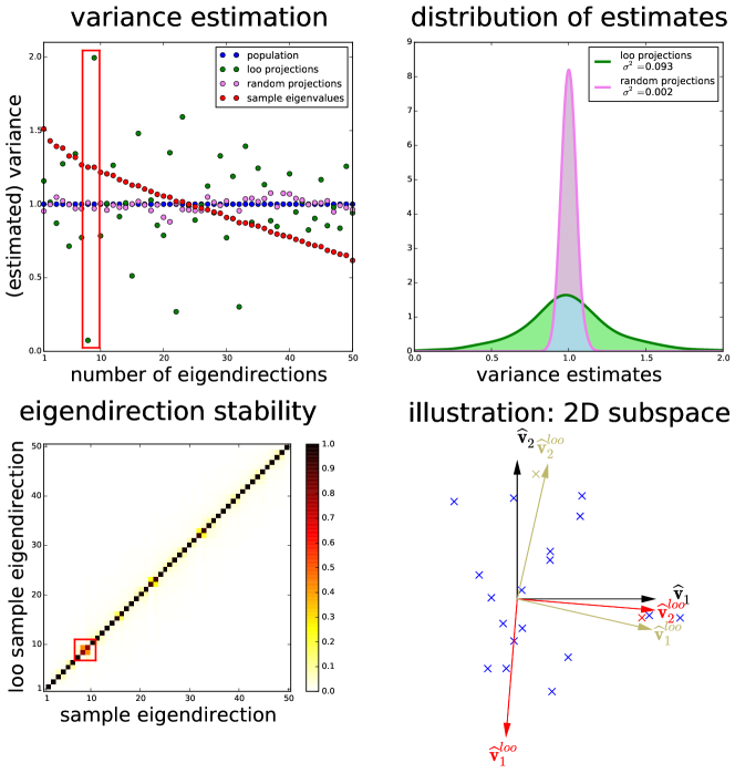
Figure 1: Illustration of the estimation error of loo-CVC.

Figure 1 illustrates the high estimation error of loo-CVC for Gaussian data with an identity population covariance ($p=50$, $n=1000$). For identity covariance, the loo-sample eigenvectors are random projections which are dependent over folds. To show the effect of this dependence, loo-sample eigenvectors are compared to projections which are entirely random.
The upper left plot shows (estimated) variances given by population and sample eigenvalues as well as estimates based on loo-CVC and random projection. It can be seen that the variance of the estimates based on loo-CVC estimates is huge compared to those based on random projections. The upper right plot shows the corresponding distributions of the variance estimates from loo-CVC and random projections (based on $R=100$ repetitions). The variances of the random projections follow a $\chi^{2}_{n}$ distribution (normalized by $n$) and hence have variance $2n^{-1}$. The variance of the loo-projections is far higher.
To explain this effect, the lower left plot shows the stability of the eigenvectors in the upper left plot, measured by the scalar product of sample eigenvectors and loo-sample eigenvectors (averaged over folds). One can see that there is a high instability of eigenvectors 8 and 9. The upper left plot shows that this is exactly where (i) the sample eigenvalues are very similar and (ii) the loo-CVC estimates deviate strongly from the population. To be precise, the loo-CVC corrections for the 8^th (larger) and 9^th (smaller) sample eigenvalues are under- and overestimated, respectively.
The plot to the lower right illustrates why this happens. It shows a subspace where both sample eigendirections $\widehat{\mathbf{v}}_{1}$ and $\widehat{\mathbf{v}}_{2}$ have very similar sample eigenvalues. Removing the yellow datapoint $\times$, with a high projection on $\widehat{\mathbf{v}}_{2}$, does not considerably change the eigendirections. We have

$$|\widehat{\mathbf{v}}_{1}^{\top}{\color[rgb]{0.7421875,0.71875,0.41796875}\widehat{\mathbf{x}}}|<|\widehat{\mathbf{v}}_{2}^{\top}{\color[rgb]{0.7421875,0.71875,0.41796875}\widehat{\mathbf{x}}}|\qquad\Rightarrow\qquad|{\color[rgb]{0.7421875,0.71875,0.41796875}\widehat{\mathbf{v}}^{\mathrm{loo}}_{1}}^{\top}{\color[rgb]{0.7421875,0.71875,0.41796875}\widehat{\mathbf{x}}}|<|{\color[rgb]{0.7421875,0.71875,0.41796875}\widehat{\mathbf{v}}^{\mathrm{loo}}_{2}}^{\top}{\color[rgb]{0.7421875,0.71875,0.41796875}\widehat{\mathbf{x}}}|.$$

Removing the red data point $$\times \widehat{\mathbf{v}}_{1} \widehat{\mathbf{v}}^{\mathrm{loo}}_{2} \times$$ with a high projection on , on the other hand, changes the eigendirections completely: now points in the direction of data point and we have

$$|\widehat{\mathbf{v}}_{2}^{\top}{\color[rgb]{1,0,0}\widehat{\mathbf{x}}}|<|\widehat{\mathbf{v}}_{1}^{\top}{\color[rgb]{1,0,0}\widehat{\mathbf{x}}}|\qquad\Rightarrow\qquad|{\color[rgb]{1,0,0}\widehat{\mathbf{v}}^{\mathrm{loo}}_{1}}^{\top}{\color[rgb]{1,0,0}\widehat{\mathbf{x}}}|<|{\color[rgb]{1,0,0}\widehat{\mathbf{v}}^{\mathrm{loo}}_{2}}^{\top}{\color[rgb]{1,0,0}\widehat{\mathbf{x}}}|.$$

It can be seen that no matter on which sample eigendirections the projection is higher, the projection on $\widehat{\mathbf{v}}^{\mathrm{loo}}_{2}$ is always higher than on $\widehat{\mathbf{v}}^{\mathrm{loo}}_{1}$. Therefore, the weaker direction has a strongly increased loo-CVC variance estimate.
A straightforward fix for this behavior is replacing loo-cross-validation by K-fold cross-validation. Using K-fold CV, it is highly unlikely that the entire set of hold-out data points has a high projection on the same eigendirection and is hence affected in the same way. This is shown in simulations after introducing isotonic regression.

loo-CVC yields eigenvalues which are not ordered. There is no reason to assume that a sample eigendirection with larger eigenvalue should have lower variance than one with smaller eigenvalue. We propose to apply isotonic regression [1]: isotonic regression searches for the decreasing sequence with minimum squared distance to the estimates:

$$({\hat{\gamma}}_{1}^{\mathrm{iso-loo-CVC}},\dots,{\hat{\gamma}}_{p}^{\mathrm{iso-loo-CVC}}) :={\operatorname*{arg\,min}}_{\mathbf{a}\in\mathbb{R}^{p}}{\sum}_{i=1}^{p}\left(a_{i}-{\hat{\gamma}}_{i}^{\mathrm{loo-CVC}}\right)^{2},$$ (13)

subject to $a_{i}>a_{i+1}$ and $\sum_{i}a_{i}=\sum_{i}{\hat{\gamma}}_{i}^{\mathrm{loo-CVC}}$. This quadratic program is reliably and quickly solved by freely available optimizers such as cvxopt, which was applied in the simulations and experiments below.

To compare CVC and NLS, the simulation shown in Figure 11 in [14] is repeated. 20%, 40% and 40% of the eigenvalues are set to 1, 3 and 10, respectively, the data is Gaussian and p/n = 1/3. Unfortunately, there is no publicly available code for NLS and we were not able to exactly reproduce the NLS performance of [14]. Our own implementation, using an open source implementation of Sequential Least Squares Programming [17, 8], is much slower and tends to get stuck in local optima. For precise estimation, it requires multiple initializations and obtained ESEs are slightly worse for large $p$.

Figure 2 compares covariance estimators $\widehat{\mathbf{C}}$ in terms of sample eigenbasis percentage improvement in average loss (SEPRIAL):

$$\text{SEPRIAL}\big{(}\widehat{\mathbf{C}}\big{)}:=100\cdot\frac{\mathbb{E}\|\widehat{\mathbf{S}}-\mathbf{S}^{\star}\|^{2}-\mathbb{E}\|\widehat{\mathbf{C}}-\mathbf{S}^{\star}\|^{2}}{\mathbb{E}\|\widehat{\mathbf{S}}-\mathbf{S}^{\star}\|^{2}}.$$

Here $\mathbf{S}^{\star}$ is the covariance matrix based on the spectrum oracle. The SEPRIAL is 100 for the spectrum oracle and zero for the sample covariance. The figure shows that loo-CVC yields very bad results, which is in line with the argumentation of the last two paragraphs. [14] reported much better results, which were only reproducable by incorporating a bug into the implementation of loo-CVC: the variance estimates of loo-CVC are calculated from projections ${\widehat{\mathbf{V}}^{\mathrm{loo}(t)}_{i}}{}^{\top}{\mathbf{x}}_{t}$ (see eq. (10)). Removing the transpose, ${\widehat{\mathbf{V}}^{\mathrm{loo}(t)}_{i}}{}{\mathbf{x}}_{t}$, defines buggy-loo-CVC which exactly yields the result reported by [14].

At first glance, it is surprising that buggy-loo-CVC is better than the correctly implemented loo-CVC. This is explained by the fact that the simulation of [14] is performed in the eigenbasis. In the eigenbasis, ${\mathbf{C}}$ is diagonal, $\widehat{\mathbf{V}}$ is approximately the identity and hence $\widehat{\mathbf{V}}^{\top}\approx\widehat{\mathbf{V}}$. Using $\widehat{\mathbf{V}}$ instead of $\widehat{\mathbf{V}}^{\top}$ has the advantage that the variance estimates do not suffer from the phenomenon illustrated in Figure 1. Randomly rotating the data before the analysis, buggy-loo-CVC breaks down completely and has much lower SEPRIAL than loo-CVC. All estimators besides buggy-loo-CVC are invariant w.r.t. the choice of basis.

The cross-validation with 10 folds in 10f-CVC yields much higher SEPRIALs than loo-CVC. Both CVC estimators profit from applying isotonic regression: iso-loo-CVC and iso-10f-CVC achieve competitive SEPRIALs compared to NLS. For a practical application, the small differences between NLS and iso-10f-CVC should be negligible.

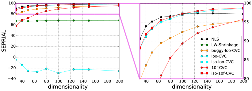
Figure 2: Estimation error of CVC estimators. Averaged over 50 repetitions.

Runtime comparison

In this section, the runtimes of CVC and NLS are compared. Both approaches are computationally more expensive than LW-Shrinkage: CVC requires multiple eigendecompositions, which are computationally expensive in high dimensions. NLS requires an expensive non-linear and non-convex optimization for the estimation of the population eigenvalues. [14] state that NLS is superior with respect to runtime, but they do not provide a numerical comparison.

To compare the runtimes of NLS and CVC, the runtimes for both iso-loo-CVC and iso-10f-CVC are measured in the same simulation setting which led to Figure 12 in [14]. As we could not obtain the original program code by Ledoit and Wolf and our implementation is much slower, a proper comparison of runtimes on the same machine is not possible. The NLS runtimes are taken from [14], the CVC results are calculated on a 2.3  GHz Intel i5 Macbook from 2011. The resulting runtimes should be roughly comparable.

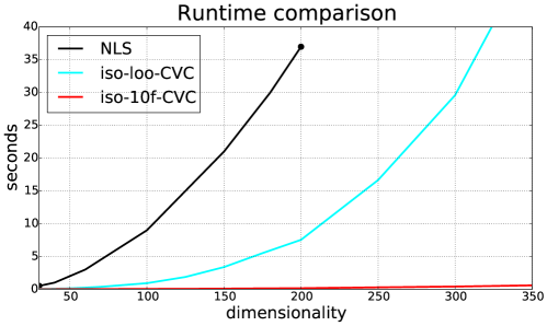
Figure 3: Runtime comparison of NLS and CVC.

Figure 3 shows that the runtime for NLS is higher than for the very slow iso-loo-CVC. The cost of iso-10f-CVC is negligible compared to the cost of NLS. Contrary to the hypothesis of Ledoit and Wolf, CVC is superior to NLS with respect to runtime.

5 Real world data

Table 1: CVC portfolio risk. Mean absolute deviations$\cdot 10^{3}$ (mean squared deviations$\cdot 10^{6}$) of the resulting portfolios for the different covariance estimators and markets. ${}^{\star}:=$ significantly better than the other models at the 5% level, tested by a randomization test.

	US	EU	HK
aoc-Shrinkage	5.41 (67.0)	3.83 (36.3)	6.11 (71.8)
DVA-FA	5.40 (66.7)	3.84 (36.0)	6.12 (71.7)
CVC	5.40 (66.7)	3.81⋆ (35.7⋆)	6.10 (71.8)

We repeat a portfolio optimization experiment from [2] and compare to DVA Factor Analysis, the covariance estimator with the best performance. In addition, we include aoc-Shrinkage, the best performing Shrinkage approach from [3]. Table 1 compares the results. Although the competing approaches explicitly model the factor structure in the data, the CVC estimator is on par for the US and HK market and even significantly reduces portfolio risk for the EU market.

As a second real world data experiment, we repeat a Neuro-Usability experiment from [3], where Linear Discriminant Analysis based on different covariance estimators is used to classify EEG recordings of noisy and noise-free phonemes. Artificial noise has been injected into one of the electrodes. In the experiment, aoc-Shrinkage outperformed other Shrinkage approaches. We include covariance matrices based on Probabilistic PCA, Factor Analysis and DVA Factor Analysis into the comparison. Table 2 shows that CVC significantly outperforms aoc-Shrinkage and the factor models. As aoc-Shrinkage, CVC is not affected by the injected noise. For the EEG data set, the factor models do not yield competitive performance: the data set does not have a pronounced factor structure.

We do not compare CVC to NLS on real world data because (i) the runtime of NLS is not feasible and (ii) the numerical stability of the optimization is not sufficient.

Table 2: CVC, Shrinkage and FM accuracies for classification tasks on the Neuro-Usability ERP-BCI data. Artificially injected noise in one electrode. ${}^{\star}:=$ significantly better than all other methods at the 5% level, tested by a randomization test.

$\sigma_{noise}$	0	10	30	100	300	1000
CVC-LDA	$\mathbf{93.74\%}^{\star}$	$\mathbf{93.73\%}^{\star}$	$\mathbf{93.73\%}^{\star}$	$\mathbf{93.73\%}^{\star}$	$\mathbf{93.73\%}^{\star}$	$\mathbf{93.73\%}^{\star}$
aoc-Shrinkage-LDA	${93.27\%}$	${93.27\%}$	${93.24\%}$	${92.88\%}$	${93.16\%}$	${93.19\%}$
PPCA-LDA	91.13%	91.15%	91.11%	91.13%	91.07%	90.85%
FA-LDA	91.61%	91.6%	91.46%	91.14%	90.4%	90.35%
DVA-FA-LDA	91.96%	91.93%	91.17%	89.44%	90.05%	89.71%

6 Summary

Spectrum correction methods keep the sample eigenvectors and only modify the eigenvalues. The state-of-the-art is Nonlinear Shrinkage (NLS), a highly complex method from Random Matrix Theory which minimizes the expected squared error. This article proposed a cross-validation-based covariance estimator (CVC) based on isotonic regression and 10-fold cross-validation which optimizes the same loss function. It yields competitive results at greatly reduced complexity and runtime.

Both NLS and CVC are computationally more complex than LW-Shrinkage. The non-linear and non-convex optimization required by NLS is very time-consuming. A comparison in the simulation setting considered by [14] showed that the cost of iso-loo-CVC is significantly smaller, although it requires $n+1$ eigendecompositions. Using ten cross-validation folds greatly reduces the computational cost and renders CVC applicable in practice. Simulations show that the estimation errors of CVC and NLS are on the same level.

On all data sets considered, the CVC estimator yields better or equal performance than state-of-the-art covariance estimators based on factor models or shrinkage. This shows that CVC is an excellent general purpose covariance estimator. The results are especially impressive as the competing methods are specifically tailored to the applications.

References

- BBBB [72] Richard E Barlow, David J Bartholomew, JM Bremner, and H Daniel Brunk. Statistical inference under order restrictions: the theory and application of isotonic regression. Wiley New York, 1972.
- BHH+ [13] Daniel Bartz, Kerr Hatrick, Christian W. Hesse, Klaus-Robert Müller, and Steven Lemm. Directional Variance Adjustment: Bias reduction in covariance matrices based on factor analysis with an application to portfolio optimization. PLoS ONE, 8(7):e67503, 07 2013.
- BM [13] Daniel Bartz and Klaus-Robert Müller. Generalizing analytic shrinkage for arbitrary covariance structures. In C.J.C. Burges, L. Bottou, M. Welling, Z. Ghahramani, and K.Q. Weinberger, editors, Advances in Neural Information Processing Systems 26, pages 1869–1877. Curran Associates, Inc., 2013.
- DGL [13] Luc Devroye, László Györfi, and Gábor Lugosi. A probabilistic theory of pattern recognition, volume 31. Springer Science & Business Media, 2013.
- DS [85] Dipak K Dey and C Srinivasan. Estimation of a covariance matrix under Stein’s loss. The Annals of Statistics, pages 1581–1591, 1985.
- EK [08] Noureddine El Karoui. Spectrum estimation for large dimensional covariance matrices using random matrix theory. Annals of Statistics, 36(6):2757–2790, 2008.
- ER [05] Alan Edelman and N. Raj Rao. Random matrix theory. Acta Numerica, 14:233–297, 2005.
- K+ [88] Dieter Kraft et al. A software package for sequential quadratic programming. DFVLR Obersfaffeuhofen, Germany, 1988.
- KR [99] Michael Kearns and Dana Ron. Algorithmic stability and sanity-check bounds for leave-one-out cross-validation. Neural Computation, 11(6):1427–1453, 1999.
- LCPB [00] Laurent Laloux, Pierre Cizeau, Marc Potters, and Jean-Phillipe Bouchaud. Random matrix theory and financial correlations. International Journal of Theoretical and Applied Finance, 3(3):391–397, 2000.
- LP [11] Olivier Ledoit and Sandrine Péché. Eigenvectors of some large sample covariance matrix ensembles. Probability Theory and Related Fields, 151(1-2):233–264, 2011.
- LW [03] Olivier Ledoit and Michael Wolf. Improved estimation of the covariance matrix of stock returns with an application to portfolio selection. Journal of Empirical Finance, 10:603–621, 2003.
- LW [04] Olivier Ledoit and Michael Wolf. A well-conditioned estimator for large-dimensional covariance matrices. Journal of Multivariate Analysis, 88(2):365–411, 2004.
- LW+ [12] Olivier Ledoit, Michael Wolf, et al. Nonlinear shrinkage estimation of large-dimensional covariance matrices. The Annals of Statistics, 40(2):1024–1060, 2012.
- LW [14] Olivier Ledoit and Michael Wolf. Spectrum estimation: A unified framework for covariance matrix estimation and pca in large dimensions. arXiv preprint arXiv:1406.6085, 2014.
- MP [67] Vladimir A. Marčenko and Leonid A. Pastur. Distribution of eigenvalues for some sets of random matrices. Mathematics of the USSR-Sbornik, 1(4):457, 1967.
- PJM [12] Ruben E Perez, Peter W Jansen, and Joaquim RRA Martins. pyopt: a python-based object-oriented framework for nonlinear constrained optimization. Structural and Multidisciplinary Optimization, 45(1):101–118, 2012.
- RPGS [02] B. Rosenow, V. Plerou, P. Gopikrishnan, and H. E. Stanley. Portfolio optimization and the random magnet problem. Europhysics Letters, 59(4):500–506, 2002.
- Sil [95] Jack W Silverstein. Strong convergence of the empirical distribution of eigenvalues of large dimensional random matrices. Journal of Multivariate Analysis, 55(2):331–339, 1995.
- Ste [56] Charles Stein. Inadmissibility of the usual estimator for the mean of a multivariate normal distribution. In Proc. 3rd Berkeley Sympos. Math. Statist. Probability, volume 1, pages 197–206, 1956.
- Ste [86] Charles Stein. Lectures on the theory of estimation of many parameters. Journal of Soviet Mathematics, 34(1):1373–1403, 1986.
- VK [82] Vladimir Naumovich Vapnik and Samuel Kotz. Estimation of dependences based on empirical data, volume 40. Springer-verlag New York, 1982.