Steady-state superradiance with Rydberg polaritons

Abstract

A steady-state superradiant laser can be used to generate ultranarrow-linewidth light, and thus has important applications in the fields of quantum information and precision metrology. However, the light produced by such a laser is still essentially classical. Here, we show that the introduction of a Rydberg medium into a cavity containing atoms with a narrow optical transition can lead to the steady-state superradiant emission of ultranarrow-linewidth non-classical light. The cavity nonlinearity induced by the Rydberg medium strongly modifies the superradiance threshold, and leads to a Mollow triplet in the cavity output spectrum—this behavior can be understood as an unusual analogue of resonance fluorescence. The cavity output spectrum has an extremely sharp central peak, with a linewidth that can be far narrower than that of a classical superradiant laser. This unprecedented spectral sharpness, together with the non-classical nature of the light, could lead to new applications in which spectrally pure quantum light is desired.

Highly stable optical frequency references play a crucial role in optical atomic clocks Hinkley et al. (2013); Bloom et al. (2014), gravitational wave detection Cagnoli et al. (2000), quantum computation Leibfried et al. (2003), and quantum optomechanics Marshall et al. (2003). Currently, the linewidth of lasers stabilized to optical reference cavities is limited by the Brownian thermomechanical noise in the cavity mirrors Numata et al. (2004); Kessler et al. (2012a, b). This fundamental thermal limit can be overcome by using a steady-state superradiant laser Haake et al. (1993); Maier et al. (2014) that works in the so-called “bad-cavity” limit, such that its lasing frequency is instead largely determined by an ultranarrow optical atomic transition Meiser et al. (2009); Bohnet et al. (2014). The insensitivity of the lasing frequency to thermal noise in the cavity mirrors allows for robust real-world applications, without the engineering of a low-vibration environment Leibrandt et al. (2011). Significant experimental progress in building superradiant lasers has recently been reported, including a proof-of-principle experiment using cold rubidium atoms Bohnet et al. (2012), and latest work using a mHz transition in cold strontium atoms Norcia and Thompson (2016); Norcia et al. (2016). These superradiant lasers all output approximately classical light.

Alternatively, nonclassical light, such as squeezed light, has found numerous applications in precision measurement Vahlbruch et al. (2016), quantum information O’Brien et al. (2009), and quantum simulation Aspuru-Guzik and Walther (2012). Here, we address the question of whether it is possible to generate nonclassical light and steady-state superradiance simultaneously, thereby achieving the benefits of both. The answer is not obvious for a number of reasons. First, a natural route towards generating non-classical light from a superradiant laser is to induce a strong nonlinearity in the cavity, which could be achieved by coupling a nonlinear medium (for example a single atom) strongly to the cavity Michler et al. (2000); Birnbaum et al. (2005). However, coupling a single atom to a cavity strongly enough can be antithetical to the bad-cavity limit required for steady-state superradiance. Second, suppose a large cavity nonlinearity has been achieved and is consistent with the bad-cavity limit. It is not a priori clear whether a strongly nonlinear cavity can support the phase synchronization of all atoms required for superradiance and spectral narrowing of the output light Xu and Holland (2015).

Remarkably, neither of these concerns turns out to pose a fundamental constraint; in this manuscript, we give a concrete example of a nonclassical (anti-bunched) light source with extremely narrow spectral linewidth, generated via steady-state superradiance. The first problem above is solved by using a Rydberg medium to generate the strong cavity nonlinearity Gorshkov et al. (2011); Peyronel et al. (2012); Firstenberg et al. (2013); Barredo et al. (2014). The major benefit of using a Rydberg medium is that one no longer requires a single atom to couple strongly to the cavity in order to generate a strong nonlinearity, making the generation of nonclassical light both more convenient and more consistent with the bad-cavity limit. The collective enhancement effect enables a sufficiently strong nonlinearity that, even for a bad cavity, the presence of more than one photon is completely blockaded; the cavity mode degenerates into a two-level system, describing the presence or absence of a single Rydberg polariton.

The second problem is addressed by a careful analysis of how superradiance works in a blockaded cavity. In a nutshell, the blockaded cavity can still synchronize the phases of the lasing atoms, although in a different parameter regime than that of a standard superradiant laser. The synchronized atoms act back on the two-level cavity as a strong and nearly coherent driving field, similar to the problem of resonance fluorescence but with the roles of atoms and light reversed [Fig. 1(a)]. An important consequence of this new physical picture is that the cavity output spectrum should consist of three peaks, the so-called Mollow triplet Mollow (1969). We verify this feature, and further demonstrate that the Mollow triplet is superimposed on an extremely sharp central peak. This peak is related to the narrow spectrum of a standard superradiant laser, but remarkably it has a quantum-limited linewidth that can be two orders of magnitude smaller for realistic experimental parameters.

Model and its implementation.—The setup we propose to achieve non-classical light from a superradiant laser is illustrated in Fig. 1(a). Two trapped ensembles of cold atoms are both coupled near-resonantly to a cavity; one serves as a Rydberg medium, and the other as a superradiant lasing medium. Experimentally, these two media can be two separately addressed parts of a single atomic ensemble.

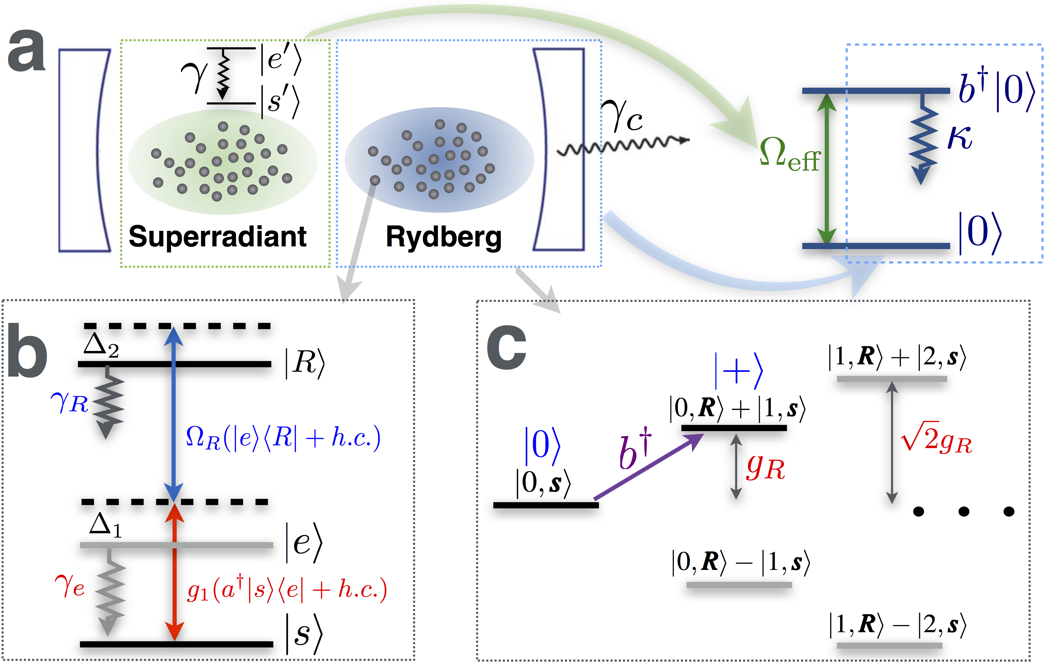
Figure 1: (Color online) (a) Schematic setup for steady-state superradiance with Rydberg polaritons. Two cold atomic ensembles are trapped inside a single-mode cavity, one used as a superradiant lasing medium and the other as a Rydberg medium. In the bad-cavity limit, a simple intuitive picture emerges in which a two-level cavity (linewidth $\kappa$) is driven near-coherently by the superradiant atoms (effective Rabi frequency $\Omega_{\text{eff}}$). $b^{\dagger}$ denotes the creation operator for the two-level cavity (or the Rydberg polariton) mode. (b) Level diagram of an atom in the Rydberg medium: $|s\rangle$, $|e\rangle$, and $|R\rangle$ denote the ground, intermediate, and Rydberg states, respectively. The $|s\rangle\leftrightarrow|e\rangle$ transition is coupled to the cavity mode $a$ with detuning $\Delta_{1}$ and coupling strength $g_{1}$. The $|e\rangle\leftrightarrow|R\rangle$ transition is driven by a laser with a two-photon detuning $\Delta_{2}$ and Rabi frequency $\Omega_{R}$. (b) Eigenstates of the Rydberg-cavity system form Jaynes-Cummings ladders. By setting the detuning of the superradiant atoms from the cavity to $g_{R}$, the superradiant atoms only couple to the $|0\rangle\leftrightarrow|+\rangle$ transition under the rotating wave approximation.

Atoms in the Rydberg medium have three relevant levels: a ground state $|s\rangle$, an excited state $|e\rangle$ (decay rate $\gamma_{e}$), and a long-lived Rydberg level $|R\rangle$ (decay rate $\gamma_{R}$), as shown in Fig. 1(b). We assume that the $|s\rangle\leftrightarrow|e\rangle$ transition is coupled to the cavity mode (decay rate $\gamma_{c}$) with uniform coupling $g_{1}$ and detuning $\Delta_{1}$, while the $|e\rangle\leftrightarrow|R\rangle$ transition is driven by a laser with Rabi frequency $\Omega_{R}$ and two-photon detuning $\Delta_{2}$. Assuming that the Rydberg state is sufficiently high-lying that all atoms are within the Rydberg blockade radius Saffman et al. (2010), only one atom can be in the state $|R\rangle$, and it is possible to reduce the Rydberg medium to a two-level super atom with a ground state $|\bm{s}\rangle=|s_{1}\cdots s_{N_{R}}\rangle$ and an excited state $|\bm{R}\rangle\equiv\frac{1}{\sqrt{N_{R}}}\sum_{i=1}^{N_{R}}|s_{1}\cdots R_{i}\cdots s_{N_{R}}\rangle$ ($N_{R}$ denotes the number of atoms in the Rydberg medium). Note that this reduction also relies on the adiabatic elimination of the intermediate state $|e_{i}\rangle$, which requires that there is much less than $1$ total atoms in state $|e\rangle$. A sufficient condition to assume is $\Delta_{1}\gg g_{1}\sqrt{N_{R}},\Omega_{R},\gamma_{R}$. With this condition met, and within the rotating wave approximation, the Rydberg-cavity system is described by the Hamiltonian $H_{R}=g_{R}(a^{\dagger}|\bm{s}\rangle\langle\bm{R}|+h.c.)$. Here $g_{R}=\sqrt{N_{R}}g_{1}\Omega_{R}/\Delta_{1}$ and $\Delta_{2}=\Omega_{R}^{2}/\Delta_{1}$ is chosen to cancel an AC stark shift, thereby bringing the cavity mode into two-photon Raman resonance with the $|\bm{s}\rangle\leftrightarrow|\bm{R}\rangle$ transition. Each eigenstate of $H_{R}$ is the superposition of state $|n,\bm{s}\rangle$ ($n$ cavity photons and no Rydberg excitation) with state $|n-1,\bm{R}\rangle$ ($n-1$ cavity photons and one Rydberg excitation), forming a Jaynes-Cummings ladder with energy shifts that increase with $n$ as $g_{R}$, $\sqrt{2}g_{R},\sqrt{3}g_{R}\cdots$ [Fig. 1(c)]. The nonlinearity in this spectrum is effectively strong if it is well resolved, requiring $g_{R}\gg\gamma_{R},\gamma_{c}$. Based on the value of $\Omega_{R}$ in existing Rydberg-EIT experiments Peyronel et al. (2012); Firstenberg et al. (2013), $g_{R}$ can be as large as a few MHz, far exceeding typical values of $\lesssim 100\>$kHz for $\gamma_{R}$ and $\gamma_{c}$ Norcia and Thompson (2016); Norcia et al. (2016).

Atoms in the superradiant medium couple to the cavity mode on a narrow-linewidth transition between ground state $|s^{\prime}\rangle$ and optically excited state $|e^{\prime}\rangle$ (decay rate $\gamma$), with uniform coupling $g_{2}$ and detuning $\delta$. The subsystem composed of the superradiant atoms and the cavity is described by the Hamiltonian $H_{S}=\frac{g_{2}}{2}\sum_{j=1}^{N}(\sigma_{j}^{+}a+\sigma_{j}^{-}a^{+})+\frac{\delta}{2}\sum_{j=1}^{N}\sigma_{j}^{z}$, where $\sigma_{j}^{+}\equiv|e^{\prime}\rangle\langle s^{\prime}|$ for the $j$th atom. By choosing $\delta=g_{R}$, the superradiant atoms only couple resonantly to the transition between the ground state $|0\rangle\equiv|0,\bm{s}\rangle$ and the Rydberg polariton state $|+\rangle\equiv(|0,\bm{R}\rangle+|1,\bm{s}\rangle)/\sqrt{2}$. Thus, under the strong-nonlinearity condition $g_{R}\gg\gamma_{c},\gamma_{R},g_{2}$, the subsystem composed of the Rydberg medium and cavity is restricted to the subspace spanned by $|0\rangle$ and $|+\rangle$. Making another rotating wave approximation, the combined system of superradiant atom, Rydberg medium, and cavity is therefore described by the effective Hamiltonian

$$H_{\text{eff}}=\frac{g}{2}\sum_{j=1}^{N}(\sigma_{j}^{-}b^{\dagger}+\sigma_{j}^{+}b).$$ (1)

Here, $g=g_{2}/\sqrt{2}$ and $b^{\dagger}\equiv|+\rangle\langle 0|$ creates a Rydberg polariton [Fig. 1(c)]. Thus we have achieved the desired model: the superradiant atoms couple to a blockaded cavity mode, or Rydberg polariton. The blockaded cavity mode contains a half photon and decays at a rate $\kappa=(\gamma_{c}+\gamma_{R})/2$, described by the Liouvillian $\mathcal{L}_{{\rm cav}}[\rho]=-\frac{\kappa}{2}(b^{\dagger}b\rho+\rho b^{\dagger}b-2b\rho b^{\dagger})$. Measurement of the mode $b$ can be carried out by directly measuring the output of the cavity mode $a$, since $a=b/\sqrt{2}$ in the subspace spanned by $|0\rangle$ and $|+\rangle$. Alternatively, one can measure $b$ by probing the Rydberg excitations inside the cavity.

Photon loss out of the cavity is countered by incoherently pumping the lasing atoms at a rate $w$, described by the Liouvillian $\mathcal{L}_{{\rm pump}}[\rho]=-\frac{w}{2}\sum_{j=1}^{N}(\sigma_{j}^{-}\sigma_{j}^{+}\rho+\rho\sigma_{j}^{-}\sigma_{j}^{+}-2\sigma_{j}^{+}\rho\sigma_{j}^{-})$. The superradiant atoms are also subject to spontaneous emission at rate $\gamma$ and dephasing at rate $\gamma_{{\rm d}}/2$. In the following analysis, we will ignore dephasing because it is not important to our main result foo , and will ignore spontaneous emission because it will be dominated by the incoherent pumping in typical experiments ($\gamma\ll w$), leading to a master equation for the full system

$$\frac{d\rho}{dt}=i[\rho,H_{\text{eff}}]+\mathcal{L}_{{\rm cav}}[\rho]+\mathcal{L}_{{\rm pump}}[\rho].$$ (2)

Similar to a standard superradiant laser, we want to operate in the bad-cavity limit where the cavity decay rate $\kappa$ is much larger than the collectively enhanced atomic decay rate $NC\gamma$ ($C\equiv g^{2}/(\kappa\gamma)$ is the single atom cooperativity) Meiser and Holland (2010a); Bohnet et al. (2012). In this limit, we will show that the cavity output inherits the narrow linewidth of the atomic transition, obtaining a frequency stability far beyond that of the cavity and the laser used to drive the Rydberg medium.

Methods of calculations.—Equation (S1) cannot be exactly solved analytically, and brute-force numerical simulation is limited to $N\lesssim 10$ atoms because the Liouville-space dimension scales as $4^{N}$. As we will show, the physics we are interested in requires large numbers of atoms, necessitating approximate analytical treatments and/or more sophisticated numerical methods. Fortunately, due to a permutation symmetry amongst the superradiant atoms, the dynamics is restricted to only a small corner of the full Liouville space, with dimension scaling only as $\sim N^{3}$ rather than $\sim 4^{N}$ Xu et al. (2013). Here, we also exploit an additional $U(1)$ phase symmetry of the coupled Rydberg-polariton and superradiant-atom system, allowing us to further reduce this scaling from $\sim N^{3}$ to $\sim N^{2}$, and thereby to perform calculations with $N$ up to several hundred. We defer the details of this new numerical algorithm to the supplemental material sup .

Since $N=10^{4}-10^{6}$ in typical experiments, we still require an approximate analytical treatment to better understand the large $N$ limit. To this end we perform a cumulant expansion, which takes into account correlations beyond mean-field theory that are crucial to the spectral properties of the cavity output Meiser et al. (2009); Meiser and Holland (2010a). The cumulant expansion is based on the intuition that, in the bad-cavity limit, higher-order correlations among the cavity and atoms are small. For example, a second-order cumulant expansion involves approximating $\langle b^{\dagger}\sigma_{1}^{-}\sigma_{2}^{z}\rangle$ by $\langle b^{\dagger}\sigma_{1}^{-}\rangle\langle\sigma_{2}^{z}\rangle$ and reduces Eq. (S1) to a closed set of coupled nonlinear equations that can be solved analytically. In the bad-cavity limit, we generally find good agreement between exact numerics performed for $N\sim 10^{2}$ and analytical solutions based on the cumulant expansion sup .

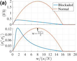
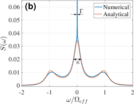
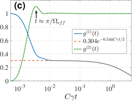
Figure 2: (Color online) (a) Comparison of the steady-state solutions for $\langle b^{\dagger}b\rangle$ and $\langle\sigma_{1}^{+}\sigma_{2}^{-}\rangle$ between the cases of a normal cavity (where $b$ is a bosonic mode) and a blockaded cavity (where $b$ is a Rydberg polariton mode). The solutions are obtained using a cumulant expansion for $N=10^{5}$ superradiant atoms and $\kappa=N^{2}C\gamma/16$ ($\tilde{\kappa}=0.25$). For the normal cavity, the superradiance peaks at $w\approx NC\gamma/2$, while for the blockaded cavity the superradiance peaks at $w\approx 1.6\kappa/N$. (b) The normalized power spectrum $S(\omega)$ of the Rydberg polariton mode from exact numerical calculations. The height of the sharp coherent scattering peak (linewidth $\Gamma$) at $\omega=0$ far exceeds the limit of the vertical axis. A Mollow triplet with splitting $\Omega_{\text{eff}}\approx Ng\langle\sigma_{1}^{+}\sigma_{2}^{-}\rangle^{1/2}$ and linewidth $\sim\kappa$ is clearly observed. The dotted line is from the analytical expression of the Mollow triplet assuming a two-level system with decay rate $\kappa$, driven with Rabi frequency $\Omega_{\text{eff}}$ by a laser (see Eq. 10.5.27 in Ref. Scully (1997)). Here $N=100$, $\kappa=NC\gamma$ and $w=2\kappa/N$. (c) Exact numerical calculations of $g^{(1)}(t)$ and $g^{(2)}(t)$ for $N=100$, $\kappa=10NC\gamma$ ($\tilde{\kappa}\approx 0.3$), and $w=1.05\kappa/N$. The long-time behavior of $g^{(1)}(t)$ matches well with the analytical expression $\langle 1-2b^{\dagger}b\rangle e^{-\Gamma t/2}$ in Eq. (4) (here $\langle 1-2b^{\dagger}b\rangle\approx 0.306$). From $g^{(2)}(t)$ we observe photon anti-bunching within a time $t\approx\pi/\Omega_{\text{eff}}$, which is the time needed to achieve a $\pi$-pulse on the two-level Rydberg polariton mode.

Superradiance in a blockaded cavity.—We define the occurrence of superradiance as when the atomic correlation function $\langle\sigma_{1}^{+}\sigma_{2}^{-}\rangle$ (equal to $\langle\sigma_{i}^{+}\sigma_{j}^{-}\rangle$ for any $i\neq j$ due to permutation symmetry) becomes finite in the large $N$ limit, thus signaling collective radiation. For a normal cavity, superradiance takes place when $w/(NC\gamma)\lesssim 1$ Meiser et al. (2009). To understand this result, we note that the cavity mode first synchronizes the phases of the atoms, creating a large collective atomic dipole. This dipole then drives photons into the cavity with an effective Rabi frequency $\Omega_{\text{eff}}\approx Ng\langle\sigma_{1}^{+}\sigma_{2}^{-}\rangle^{1/2}$, creating a photon flux $\kappa(\Omega_{\text{eff}}/\kappa)^{2}\approx N^{2}C\gamma\langle\sigma_{1}^{+}\sigma_{2}^{-}\rangle$. Because $H_{\text{eff}}$ conserves the total number of photons and atomic excitations, in steady state this photon flux should equal the single-atom pumping rate $w$ times the number of atoms in the ground state, $Nw\langle 1-\sigma_{1}^{z}\rangle/2$. It can be shown that the maximum value of $\langle\sigma_{1}^{+}\sigma_{2}^{-}\rangle$ is $1/8$ under incoherent pumping, with a corresponding $\langle\sigma_{1}^{z}\rangle=1/2$ Meiser and Holland (2010b). Thus $w=NC\gamma/2$ maximizes the collective radiation [see Fig. 2(a)].

If one operates very deeply in the bad-cavity limit, such that $\kappa\gg N^{2}C\gamma$, then $\langle b^{\dagger}b\rangle=N^{2}C\gamma\langle\sigma_{1}^{+}\sigma_{2}^{-}\rangle/\kappa\ll 1$ and the photon blockade becomes irrelevant. We are instead interested in the situation $NC\gamma\ll\kappa\ll N^{2}C\gamma$. This regime is readily achievable in current experiment Bohnet et al. (2012); Norcia and Thompson (2016); Norcia et al. (2016), and ensures both the bad-cavity limit and a strong blockade effect, since $\langle b^{\dagger}b\rangle\gg 1$ in the absence of a blockade. For convenience, we define a dimensionless parameter $\tilde{\kappa}\equiv[\kappa/(N^{2}C\gamma)]^{1/2}=\kappa/(Ng)$, and restrict our analysis to $1/\sqrt{N}\ll\tilde{\kappa}\ll 1$.

For a blockaded cavity, we find that superradiance instead takes place when $w\sim\kappa/N=g\tilde{\kappa}$ [Fig. 2(a)]; comparing to the result $w\sim NC\gamma=g/\tilde{\kappa}$ for a normal cavity, we see that superradiance now occurs at a much smaller pumping rate. This is because the collective dipole formed by the superradiant atoms is now driving a two-level cavity, which saturates ($\langle b^{\dagger}b\rangle\rightarrow 1/2$) when $\Omega_{\text{eff}}\gg\kappa$. As before, since $H_{\text{eff}}$ conserves the sum of photonic and atomic excitations, detailed balance requires $Nw\langle 1-\sigma_{1}^{z}\rangle/2=\kappa\langle b^{\dagger}b\rangle$; thus $w\approx 2\kappa/N$ is necessary to maximize the collective radiation. Formally, our analytical solution based on the cumulant expansion shows that in the large $N$ limit,

$$\langle b^{\dagger}b\rangle\approx\frac{1}{4}\Big{(}1+\tilde{w}-\sqrt{(1-\tilde{w})^{2}+4\tilde{w}^{2}\tilde{\kappa}^{2}}\,\,\Big{)}$$ (3)

with $\tilde{w}\equiv w(N/\kappa)$ defined as a dimensionless pumping rate. Thus the photon flux is maximized when $\tilde{w}\approx 2/(1+4\tilde{\kappa}^{2})\approx 2$, or $w\approx 2\kappa/N$, consistent with the above argument.

Next, we turn to the spectral properties of the cavity output. Figure 2(b) shows the results of a numerical calculation of the normalized power spectrum $S(\omega)=\frac{1}{2\pi}\int_{-\infty}^{\infty}g^{(1)}(t)e^{i\omega t}dt$, with $g^{(1)}(t)\equiv\langle b^{\dagger}(t)b(0)\rangle/\langle b^{\dagger}b\rangle$ (assuming steady state is reached at $t=0$). Remarkably, $S(\omega)$ is very similar to the resonance-fluorescence spectrum of a two-level atom with linewidth $\kappa$, driven by a laser with Rabi frequency $\Omega_{\text{eff}}$ and a small linewidth $\Gamma\ll\kappa$ Scully (1997). In particular, a Mollow triplet is observed with splittings of $\approx\Omega_{\text{eff}}$ between three peaks of width $\sim\kappa$. In addition, there is a sharp peak (linewidth $\Gamma\ll\kappa$) at $\omega=0$, arising from the coherent scattering of the collective atomic dipole off the blockaded cavity.

To determine $\Gamma$, we use the quantum regression theorem together with the cumulant expansion sup to analytically calculate $g^{(1)}(t)$ in the large $N$ limit, obtaining

$$g^{(1)}(t) \approx\langle 1-2b^{\dagger}b\rangle e^{-\Gamma t/2}+\langle 2b^{\dagger}b\rangle e^{-\kappa t/2},$$ (4)

$$\Gamma \approx C\gamma\sqrt{(1-\tilde{w})^{2}+4\tilde{w}^{2}\tilde{\kappa}^{2}}.$$ (5)

As shown in Fig. 2(c), the long-time behavior of $g^{(1)}(t)$ in the above solution agrees well with exact numerical calculations, allowing us to reliably extract $\Gamma$ from Eq. (5) for large $N$ (due to higher-order correlations ignored in the cumulant expansion, Eq. (4) is not accurate for $t\lesssim 1/\kappa$).

According to Eq. (5), $\Gamma$ is minimized at $\tilde{w}=1$, achieving $\Gamma_{\min}=2\tilde{\kappa}C\gamma$. This is a surprising and important result, because without photon blockade, the linewidth of the cavity output is at least $C\gamma$ Meiser et al. (2009). In fact, $C\gamma$ is the smallest energy scale in the full system, but the photon blockade effect has led to a new energy scale that is parametrically smaller in $\tilde{\kappa}$. Because $1/\sqrt{N}\ll\tilde{\kappa}\ll 1$, the central linewidth can be up to $100$ times smaller than that of a classical superradiant laser for $N=10^{6}$ lasing atoms. Meanwhile, the photon flux is nearly maximized ($\langle b^{\dagger}b\rangle\approx(1-\tilde{\kappa})/2\approx 1/2$), and the output light is nonclassical due to the nonlinearity of the cavity. In particular, clear anti-bunching can be seen by plotting $g^{(2)}(t)\equiv\langle b^{\dagger}(0)b^{\dagger}(t)b(t)b(0)\rangle/\langle b^{\dagger}b\rangle^{2}$ [see Fig. 2(c)], and occurs because a Rabi oscillation time $t\approx\pi/\Omega_{\text{eff}}$ is required to refill the blockaded cavity after photon emission.

One speculative explanation for the blockade-induced linewidth narrowing is as follows. For a normal cavity, $\Gamma=C\gamma=g^{2}/\kappa$ can be understood by adiabatically eliminating the cavity, which is well justified in the bad-cavity limit. For a blockaded cavity, this adiabatic elimination is not strictly justified, because it masks the correlations induced by the photon blockade. However, the blockade effect can be captured by renormalizing $C\gamma$ by a factor $\langle 1-2b^{\dagger}b\rangle$ originating from the commutation relation $[b,b^{\dagger}]=1-2b^{\dagger}b$ of the blockaded cavity mode $b$, in contrast to the $[a,a^{\dagger}]=1$ of the normal cavity mode $a$. Physically, this can be interpreted as a suppression of the cavity-mediated spontaneous emission by the blockade effect, which prohibits successive emissions. In the limit of a strong blockade effect, $\tilde{\kappa}\ll 1$, we indeed find that Eqs. (3) and (5) lead to $\Gamma\approx C\gamma\langle 1-2b^{\dagger}b\rangle$.

Finally, we note that the linewidth reduction attributable to the photon blockade comes with a tradeoff. The fraction of the power contained within the narrow-linewidth spectral component is also given by the small factor $\langle 1-2b^{\dagger}b\rangle$, as can be seen from Eq. (4). One can transfer this narrow but low-power spectral component to a high-power laser via a homodyne phase lock. However, the requirement to detect many photons within a time given by the inverse bandwidth of the phase-lock feedback loop makes the requirements on prestabilization of the high-power laser’s frequency more severe.

Outlook.—We envision a proof-of-principle experiment similar to Ref. Bohnet et al. (2012) in the near future where a Raman transition in cold Rb atoms is used to produce a tunable lasing transition linewidth $\gamma$, making the parameter regime required in our proposal more readily accessible. The photon blockade could be obtained by driving a Rydberg transition in a sub-ensemble of the Rb atoms Firstenberg et al. (2013). The modified superradiant threshold, narrower linewidth, and nonclassical character of the emitted light can be observed by measuring the photon flux, $g^{(1)}(t)$, and $g^{(2)}(t)$ at the cavity output. By tuning the strength and range of interactions among the Rydberg states, one may be able to engineer more general forms of nonclassical light (beyond simple anti-bunching), while maintaining the spectral sharpness by staying in the superradiant regime. We expect such nonclassical light to become useful in a variety of future applications, including sub shot-noise spectroscopy Kim et al. (2001); Teich and Saleh (1990), quantum networks of optical clocks Komar et al. (2014), and realizations of fractional quantum Hall states Hafezi et al. (2013); Kapit and Simon (2013).

Supplemental Material for “Steady-state superradiance with Rydberg polaritons”

This supplemental material provides technical details for the numerical and the cumulant expansion methods used in solving Eq. (2) of the main text. For completeness, we rewrite Eq. (2) of the main text, this time including terms associated with dephasing ($\mathcal{L}_{{\rm deph}}$) and spontaneous emission ($\mathcal{L}_{{\rm spont}}$) of the lasing atoms:

$$\frac{d\rho}{dt} =i[\rho,H_{\text{eff}}]+\mathcal{L}_{{\rm cav}}[\rho]+\mathcal{L}_{{\rm pump}}[\rho]+\mathcal{L}_{{\rm spont}}[\rho]+\mathcal{L}_{{\rm deph}}[\rho],$$ (S1)

$$H_{\text{eff}} =\frac{g}{2}\sum_{j=1}^{N}(\sigma_{j}^{+}b+\sigma_{j}^{-}b^{\dagger}),$$ (S2)

$$\mathcal{L}_{{\rm cav}}[\rho] =-\frac{\kappa}{2}(b^{\dagger}b\rho+\rho b^{\dagger}b-2b\rho b^{\dagger}),$$ (S3)

$$\mathcal{L}_{{\rm pump}}[\rho] =-\frac{w}{2}\sum_{j=1}^{N}(\sigma_{j}^{-}\sigma_{j}^{+}\rho+\rho\sigma_{j}^{-}\sigma_{j}^{+}-2\sigma_{j}^{+}\rho\sigma_{j}^{-}),$$ (S4)

$$\mathcal{L}_{{\rm spont}}[\rho] =-\frac{\gamma}{2}\sum_{j=1}^{N}(\sigma_{j}^{+}\sigma_{j}^{-}\rho+\rho\sigma_{j}^{+}\sigma_{j}^{-}-2\sigma_{j}^{-}\rho\sigma_{j}^{+}),$$ (S5)

$$\mathcal{L}_{{\rm deph}}[\rho] =-\frac{\gamma_{d}}{4}\sum_{j=1}^{N}(\rho-\sigma_{j}^{z}\rho\sigma_{j}^{z}),$$ (S6)

where $\sigma_{j}s$ are the Pauli matrices for the lasing atoms, and $b$ is the blockaded cavity mode.

Two important symmetries that can greatly simplify our calculations exist in the above master equation: The first is the permutation symmetry among all of the atoms, and the second is the $U(1)$ symmetry associated with invariance under the simultaneous transformations $\sigma_{j}^{-}\rightarrow\sigma_{j}^{-}e^{i\phi}$ (for all $j$s) and $b\rightarrow be^{i\phi}$. In a typical experiment, the initial state of the atoms and cavity breaks neither the permutation nor the $U(1)$ symmetry, thus at any time during the state evolution we will assume $\langle\sigma_{j}^{-}\rangle=0$ for all $j$s and $\langle b\rangle=0$.

I Cumulant expansion Method

The second-order cumulant expansion allows us to make the following approximations $\langle b^{\dagger}\sigma_{1}^{-}\sigma_{2}^{z}\rangle\approx\langle b^{\dagger}\sigma_{1}^{-}\rangle\langle\sigma_{2}^{z}\rangle$, $\langle\sigma_{1}^{-}\sigma_{2}^{+}b^{\dagger}b\rangle\approx\langle\sigma_{1}^{-}\sigma_{2}^{+}\rangle\langle b^{\dagger}b\rangle$, and $\langle b^{\dagger}b\sigma_{1}^{z}\rangle\approx\langle b^{\dagger}b\rangle\langle\sigma_{1}^{z}\rangle$. With these approximations, the equations of motion for $\langle\sigma_{1}^{z}\rangle$, $\langle\sigma_{1}^{+}\sigma_{2}^{-}\rangle$, $\langle b^{\dagger}b\rangle$, and $\langle b^{\dagger}\sigma_{1}^{-}\rangle$ form the following closed set:

$$\frac{d\langle\sigma_{1}^{z}\rangle}{dt} =i\left(\langle b^{\dagger}\sigma_{1}^{-}\rangle-\langle b\sigma_{1}^{+}\rangle\right)-(w+\gamma)\langle\sigma_{1}^{z}\rangle+(w-\gamma),$$ (S7)

$$\frac{d\langle\sigma_{1}^{+}\sigma_{2}^{-}\rangle}{dt} \approx\frac{g\langle\sigma_{1}^{z}\rangle}{2i}\left(\langle b^{\dagger}\sigma_{1}^{-}\rangle-\langle\sigma_{1}^{+}b\rangle\right)-(w+\gamma+\gamma_{d})\langle\sigma_{1}^{+}\sigma_{2}^{-}\rangle,$$ (S8)

$$\frac{d\langle b^{\dagger}b\rangle}{dt} =\frac{Ng}{2i}\left(\langle b^{\dagger}\sigma_{1}^{-}\rangle-\langle\sigma_{1}^{+}b\rangle\right)-\kappa\langle b^{\dagger}b\rangle,$$ (S9)

$$\frac{d\langle b^{\dagger}\sigma_{1}^{-}\rangle}{dt} \approx\frac{ig}{2}\left\{\left[(N-1)\langle\sigma_{1}^{-}\sigma_{2}^{+}\rangle+\frac{\langle\sigma_{z}\rangle+1}{2}\right]\langle 1-2b^{\dagger}b\rangle+\langle b^{\dagger}b\rangle\langle\sigma_{1}^{z}\rangle\right\}-\frac{w+\kappa+\gamma+\gamma_{d}}{2}\langle b^{\dagger}\sigma_{1}^{-}\rangle.$$ (S10)

Steady-state values of $\langle\sigma_{1}^{z}\rangle$, $\langle\sigma_{1}^{+}\sigma_{2}^{-}\rangle$, $\langle b^{\dagger}b\rangle$, and $\langle b^{\dagger}\sigma_{1}^{-}\rangle$ are obtained by setting the l.h.s. of Eqs. (S7-S10) to zero. To obtain the spectral properties of the cavity output, we use the quantum regression theorem Walls (2011) to calculate $\langle b^{\dagger}(t)b(0)\rangle$,

$$\frac{d}{dt}\begin{pmatrix}b^{\dagger}(t)b(0)\\ \sigma_{1}^{+}(t)b(0)\end{pmatrix}\approx\begin{pmatrix}-\frac{\kappa}{2}&\frac{iNg}{2}\langle 1-2b^{\dagger}b\rangle\\ -\frac{ig}{2}\langle\sigma_{1}^{z}\rangle&-\frac{w+\gamma+\gamma_{d}}{2}\end{pmatrix}\begin{pmatrix}b^{\dagger}(t)b(0)\\ \sigma_{1}^{+}(t)b(0)\end{pmatrix}.$$ (S11)

Here equal-time steady-state expectation values are implied unless two time arguments are explicitly shown. We have also made additional approximations based on the cumulant expansion, such as $\langle b^{\dagger}(t)b(0)\sigma_{1}^{z}\rangle\approx\langle b^{\dagger}(t)b(0)\rangle\langle\sigma_{1}^{z}\rangle$.

The approximations made above are justified by good agreement between the solutions of Eqs. (S7-S11) and exact numerical calculations of Eq. (S1) when $\kappa\gg NC\gamma$ (the bad-cavity limit) and $t\gg 1/\kappa$ in $\langle b^{\dagger}(t)b(0)\rangle$ (see Fig. S1).

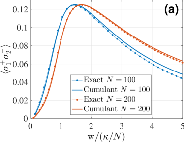
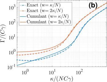
Figure S1: (Color online) Comparison between exact numerical calculations and analytical calculations using the second-order cumulant expansion. (a) The steady-state value of $\langle\sigma_{1}^{+}\sigma_{2}^{-}\rangle$ as a function of pumping rate $w$ for $\kappa=10NC\gamma$. Better agreement is observed for larger $N$. (b) The linewidth $\Gamma$ fitted from the long-time ($t\gg 1/\kappa$) exponential decay in $\langle b^{\dagger}(t)b(0)\rangle$ as a function of $\kappa$ for $N=100$. Good agreement is found for $\kappa\gg NC\gamma$.

II Numerical Method

We now present a highly efficient numerical method for solving Eq. (S1). Our numerical method can actually be applied to any cavity-QED master equation that has the aforementioned permutation symmetry and $U(1)$ symmetry. Thus in the following, we will assume a more general situation where the cavity mode has at most $M$ photons. The fully blockaded cavity can be studied by setting $M=1$, whereas a normal (harmonic) cavity mode or a cavity mode with a generic form of nonlinearity can be studied by assuming a sufficiently large $M$. To avoid confusion in notations, below we will call this general cavity mode $a$ as $b$ is reserved for the blockaded cavity mode.

In the presence of dissipative processes, exploiting either the permutation or the $U(1)$ symmetry numerically is nontrivial. For example, unlike in the case of coherent dynamics, permutation symmetry does not imply a restriction of dynamics to the well-known Dicke-state basis, because the Liouvillians Eqs. (S4-S6) can couple states within the Dicke-subspace to states outside of it Hartmann . In addition, although the aforementioned $U(1)$ symmetry guarantees that the Hamiltonian $H_{\text{eff}}$ conserves the total number of atomic and cavity excitations (i.e. $a^{\dagger}a+\sum_{j=1}^{N}\sigma_{j}^{z}$), this symmetry does not imply such a conservation law for dissipative dynamics. To correctly make use of both symmetries, we start by constructing the following basis states for the density matrix:

$$\rho_{(N_{+},N_{-},N_{Z},N_{a^{\dagger}},N_{a})} = \Big{(}\frac{1}{2^{N}N!}\text{$\sum$}_{\mathcal{P}}(\sigma_{1}^{+}\otimes\cdots\otimes\sigma_{N_{+}}^{+}\otimes\sigma_{N_{+}+1}^{-}\otimes\cdots\otimes\sigma_{N_{+}+N_{-}}^{-}$$ (S13)

$$\otimes\sigma_{N_{+}+N_{-}+1}^{z}\otimes\cdots\sigma_{N_{+}+N_{-}+N_{Z}}^{z}\otimes I_{N_{+}+N_{-}+N_{Z}+1}\otimes\cdots\otimes I_{N}\Big{)}\otimes(a^{\dagger})^{N_{a^{\dagger}}}a^{N_{a}},$$

where the notation $\sum_{\mathcal{P}}$ denotes the summation over all permutations of the atomic indices $1,2,\cdots N$. The indices $(N_{+},N_{-},N_{Z},N_{a^{\dagger}},N_{a})$ specify how many $(\sigma_{i}^{+},\sigma_{i}^{-},\sigma_{i}^{z},a^{\dagger},a)$ appear in the above basis state. Assuming that the initial state of the atoms is invariant under permutations, then at any time $t$, we can express $\rho(t)$ as

$$\rho(t)=\sum_{N_{+},N_{-},N_{Z},N_{a},N_{a^{\dagger}}}c_{(N_{+},N_{-},N_{Z},N_{a^{\dagger}},N_{a})}(t)\rho_{(N_{+},N_{-},N_{Z},N_{a^{\dagger}},N_{a})}.$$ (S14)

This choice of basis states allows us to exploit the $U(1)$ symmetry easily, because the invariance of $\rho(t)$ under the transformation $\sigma_{j}^{+}\rightarrow\sigma_{j}^{+}e^{i\phi}$ and $a^{\dagger}\rightarrow a^{\dagger}e^{i\phi}$ implies that

$$\delta N=N_{+}+N_{a^{\dagger}}-N_{-}-N_{a}$$ (S15)

is a conserved quantity. The physical meaning of this conserved quantity is that, although the environment can change the total number of atomic and photonic excitations, it cannot build up coherence among states with different total number of excitations. Since we assume an initial state with $\langle a\rangle=\langle\sigma_{j}^{-}\rangle=0$, $\rho(t)$ will be restricted to the $\delta N=0$ subspace.

Together with the natural constraint $N_{+}+N_{-}+N_{Z}\leq N$, $N_{a^{\dagger}},N_{a}\leq M$, we have reduced the Liouville-space dimension from $4^{N}(M+1)^{2}$ to only $\sim N^{2}(M+1)^{2}$, making efficient numerical calculations possible. To write down a numerical algorithm, we still need to find explicit representations of the initial state and the Liouvillian superoperators in this basis set.

II.1 Normalization and initial state

Because the Pauli matrices are traceless, only the basis states with $N_{+}=N_{-}=N_{Z}=0$ have nonzero trace with respect to the atomic Hilbert space, and the trace of such a state over the atomic Hilbert space is $1$ due to the normalization factor in Eq. (S13). In addition, only basis states with $N_{a}=N_{a^{\dagger}}$ have nonzero trace with respect to the photonic Hilbert space, and the trace for a basis state with $N_{a}=N_{a^{\dagger}}=m$ over the truncated photonic Hilbert space is given by

$$\text{Tr}[(a^{\dagger})^{m}a^{m}]=\sum_{n=m}^{M}\frac{n!}{(n-m)!}=(M+1)M\cdots(M+1-m)/(m+1)\equiv P_{m}.$$ (S16)

As a result, a normalized initial state must satisfy $\text{Tr}[\rho(t)]=\sum_{m=0}^{M}c_{(0,0,0,m,m)}(t)P_{m}=1.$ For simplicity, we will choose our initial state to be a completely mixed state proportional to an identity matrix: $\rho(0)=c_{(0,0,0,0,0)}(0)\rho_{(0,0,0,0,0)}$, with $c_{(0,0,0,0,0)}(0)=1/P_{0}=\frac{1}{M+1}$.

II.2 Matrix elements for cavity operators

We will now find the matrix elements for the cavity operators by writing down the rules for applying $a$ and $a^{\dagger}$ on the left or the right side of the basis state $\rho_{(N_{+},N_{-},N_{Z},N_{a^{\dagger}},N_{a})}$. For notational simplicity, we will ignore the $(N_{+},N_{-},N_{Z})$ indices here because the cavity operators cannot change them. Since $\rho_{(N_{a^{\dagger}},N_{a})}\equiv(a^{\dagger})^{N_{a^{\dagger}}}a^{N_{a}}$ is normal ordered, the operations that preserve the normal ordering are simple:

$$\rho_{(N_{a^{\dagger}},N_{a})}a =\rho_{(N_{a^{\dagger}},N_{a}+1)},$$ (S17)

$$a^{\dagger}\rho_{(N_{a^{\dagger}},N_{a})} =\rho_{(N_{a^{\dagger}}+1,N_{a})}.$$ (S18)

A complication arises when we need to bring $a\rho_{(N_{a^{\dagger}},N_{a})}=a(a^{\dagger})^{N_{a^{\dagger}}}a^{N_{a}}$ into the normal order, particularly since $[a,a^{\dagger}]\neq 1$ (because the cavity Hilbert space is truncated to a maximum of $M$ photons). Within the truncated Hilbert space, it can be shown that $[a,a^{\dagger}]=1-\frac{M+1}{M!}(a^{\dagger})^{M}a^{M}.$ Using this commutation relation repeatedly gives us

$$\rho_{(N_{a^{\dagger}},N_{a})}a^{\dagger} =\rho_{(N_{a^{\dagger}}+1,N_{a})}+N_{a}\rho_{(N_{a^{\dagger}},N_{a}-1)}-\frac{M+1}{(M-N_{a}+1)!}\rho_{(M+1+N_{a^{\dagger}}-N_{a},M)},$$ (S19)

$$a\rho_{(N_{a^{\dagger}},N_{a})} =\rho_{(N_{a^{\dagger}},N_{a}+1)}+N_{a^{\dagger}}\rho_{(N_{a^{\dagger}}-1,N_{a})}-\frac{M+1}{(M-N_{a^{\dagger}}+1)!}\rho_{(M,M+1+N_{a}-N_{a^{\dagger}})},$$ (S20)

where we implicitly assume (here and in everything that follows) that any indices $N_{a^{\dagger}},N_{a}$ in a basis state $\rho_{(N_{a^{\dagger}},N_{a})}$ should lie between $0$ and $M$, otherwise we need to drop such an “illegal” basis state because it will be annihilated by either $a$ or $a^{\dagger}$. Eqs. (S17-S20) will allow us to construct all terms in $\mathcal{L}_{{\rm cav}}[\rho]$.

II.3 Matrix elements for atomic operators

The matrix elements for the atomic operators can be determined in a similar manner. For simplicity, here we ignore the $(N_{a^{\dagger}},N_{a})$ indices in specifying the basis state $\rho_{(N_{+},N_{-},N_{Z},N_{a^{\dagger}},N_{a})}$ as the atomic operators cannot change the quantum numbers $N_{a}$ and $N_{a^{\dagger}}$. Let us start with the collective atomic operators $\sigma^{\pm}=\sum_{i}\sigma_{i}^{\pm}$ and $\sigma^{z}=\sum_{i}\sigma_{i}^{z}$, which obey

$$\sigma^{+}\rho_{(N_{+},N_{-},N_{Z})} =\frac{1}{2}N_{-}[\rho_{(N_{+},N_{-}-1,N_{Z})}+\rho_{(N_{+},N_{-}-1,N_{Z}+1)}]-N_{Z}\rho_{(N_{+}+1,N_{-},N_{Z}-1)}+N_{I}\rho_{(N_{+}+1,N_{-},N_{Z}),}$$ (S21)

$$\rho_{(N_{+},N_{-},N_{Z})}\sigma^{+} =\frac{1}{2}N_{-}[\rho_{(N_{+},N_{-}-1,N_{Z})}-\rho_{(N_{+},N_{-}-1,N_{Z}+1)}]+N_{Z}\rho_{(N_{+}+1,N_{-},N_{Z}-1)}+N_{I}\rho_{(N_{+}+1,N_{-},N_{Z})},$$ (S22)

$$\sigma^{-}\rho_{(N_{+},N_{-},N_{Z})} =\frac{1}{2}N_{+}[\rho_{(N_{+}-1,N_{-},N_{Z})}-\rho_{(N_{+}-1,N_{-},N_{Z}+1)}]+N_{Z}\rho_{(N_{+},N_{-}+1,N_{Z}-1)}+N_{I}\rho_{(N,N_{-}+1,N_{Z})},$$ (S23)

$$\rho_{(N_{+},N_{-},N_{Z})}\sigma^{-} =\frac{1}{2}N_{+}[\rho_{(N_{+}-1,N_{-},N_{Z})}+\rho_{(N_{+}-1,N_{-},N_{Z}+1)}]-N_{Z}\rho_{(N_{+},N_{-}+1,N_{Z}-1)}+N_{I}\rho_{(N,N_{-}+1,N_{Z})},$$ (S24)

$$\sigma^{z}\rho_{(N_{+},N_{-},N_{Z})} =(N_{+}-N_{-})\rho_{(N_{+},N_{-},N_{Z})}+N_{Z}\rho_{(N_{+},N_{-},N_{Z}-1)}+N_{I}\rho_{(N_{+},N_{-},N_{Z}+1)},$$ (S25)

$$\rho_{(N_{+},N_{-},N_{Z})}\sigma^{z} =(N_{-}-N_{+})\rho_{(N_{+},N_{-},N_{Z})}+N_{Z}\rho_{(N_{+},N_{-},N_{Z}-1)}+N_{I}\rho_{(N_{+},N_{-},N_{Z}+1)}.$$ (S26)

Again we have implicitly assumed that the indices $N_{+}$, $N_{-}$, and $N_{Z}$ in a basis state $\rho_{(N_{+},N_{-},N_{Z})}$ should lie between $0$ and $N$ and satisfy $N_{+}+N_{-}+N_{Z}\leq N$, otherwise we will drop the illegal basis state. The recycling terms in $\mathcal{L}_{{\rm spont}}$ and $\mathcal{L}_{{\rm pump}}$ cannot be written in terms of collective atomic operators, and must be treated separately; we find

$$2\sum_{j=1}^{N}\sigma_{j}^{-}\rho_{(N_{+},N_{-},N_{Z})}\sigma_{j}^{+} =(N_{I}-N_{Z})\rho_{(N_{+},N_{-},N_{Z})}+N_{Z}\rho_{(N_{+},N_{-},N_{Z}-1)}-N_{I}\rho_{(N_{+},N_{-},N_{Z}+1),}$$ (S27)

$$2\sum_{j=1}^{N}\sigma_{j}^{+}\rho_{(N_{+},N_{-},N_{Z})}\sigma_{j}^{-} =(N_{I}-N_{Z})\rho_{(N_{+},N_{-},N_{Z})}-N_{Z}\rho_{(N_{+},N_{-},N_{Z}-1)}+N_{I}\rho_{(N_{+},N_{-},N_{Z}+1)}.$$ (S28)

These rules enable us to construct the matrices for $\mathcal{L}_{{\rm spont}}[\rho]$, $\mathcal{L}_{{\rm pump}}[\rho]$, and $\mathcal{L}_{{\rm deph}}[\rho]$, and combined with the rules for application of cavity operators we can also construct the representation of $H_{\text{eff}}$.

II.4 Measurement

The expectation value of most observables we are interested in can be calculated very efficiently without the need of writing down the matrices for them. For example, to calculate $\langle\sigma^{z}\rangle$ we can use the rule in Eq. (S25) and the fact that only the $N_{+}=N_{-}=N_{Z}=0,\thinspace N_{a^{\dagger}}=N_{a}$ basis states have nonzero trace:

$$\text{Tr}[\sigma^{z}\rho(t)]=\sum_{m=0}^{M}c_{(0,0,1,m,m)}(t)P_{m}.$$ (S29)

Similarly, we can calculate $\langle\sigma_{i}^{+}\sigma_{j}^{-}\rangle$ and $\langle a^{\dagger}a\rangle$ using

$$\text{Tr}[\sigma_{i}^{+}\sigma_{j}^{-}\rho(t)] =\text{Tr}[\frac{\sigma^{+}\sigma^{-}-(1+\sigma^{z})/2}{N(N-1)}\rho(t)]=\sum_{m=0}^{N}c_{(1,1,0,m,m)}(t)P_{m}/[4N(N-1)],$$ (S30)

$$\text{Tr}[a^{\dagger}a\rho(t)] =\sum_{m=0}^{M}c_{(0,0,0,m,m)}(t)\text{Tr}[\rho_{(0,0,0,m+1,m+1)}+m\rho_{(0,0,0,m,m)}]=\sum_{m=0}^{M-1}c_{(0,0,0,m,m)}P_{m+1}+\sum_{m=0}^{M}c_{(0,0,0,m,m)}mP_{m}.$$ (S31)

The calculation of the two-time correlation $g^{(1)}(\tau)=\langle a^{\dagger}(t+\tau)a(t)\rangle/\langle a^{\dagger}(t)a(t)\rangle$ is more complicated. We need to first find $\rho^{\prime}(t)=a\rho(t)$, which is in the $\delta N=1$ subspace and requires a new set of basis states $\{\rho_{(N_{+},N_{-},N_{Z},N_{a^{\dagger}},N_{a})}\}$ with $\delta N=1$ to be represented. Next, we evolve the master equation [Eq. (S1)] for time $\tau$ using $\rho^{\prime}(t)$ as the initial state, and measure $a^{\dagger}(t+\tau)$:

$$\langle a^{\dagger}(t+\tau)a(t)\rangle=\text{Tr}[a^{\dagger}\rho^{\prime}(t+\tau)]=\sum_{m=0}^{M-1}c_{(0,0,0,m+1,m)}^{\prime}(t+\tau)P_{m+1}.$$ (S32)

References

Hinkley et al. (2013)N. Hinkley, J. A. Sherman, N. B. Phillips, M. Schioppo,
N. D. Lemke, K. Beloy, M. Pizzocaro, C. W. Oates, and A. D. Ludlow, Science 341, 1215
(2013).
Bloom et al. (2014)B. J. Bloom, T. L. Nicholson, J. R. Williams, S. L. Campbell, M. Bishof,
X. Zhang, W. Zhang, S. L. Bromley, and J. Ye, Nature 506, 71 (2014).
Cagnoli et al. (2000)G. Cagnoli, L. Gammaitoni,
J. Hough, J. Kovalik, S. McIntosh, M. Punturo, and S. Rowan, Phys. Rev. Lett. 85, 2442 (2000).
Kessler et al. (2012b)T. Kessler, C. Hagemann,
C. Grebing, T. Legero, U. Sterr, F. Riehle, M. J. Martin, L. Chen, and J. Ye, Nat. Photonics 6, 687 (2012b).
Peyronel et al. (2012)T. Peyronel, O. Firstenberg, Q.-Y. Liang, S. Hofferberth,
A. V. Gorshkov, T. Pohl, M. D. Lukin, and V. Vuletić, Nature 488, 57 (2012).
Firstenberg et al. (2013)O. Firstenberg, T. Peyronel, Q.-Y. Liang,
A. V. Gorshkov, M. D. Lukin, and V. Vuletić, Nature 502, 71 (2013).
Barredo et al. (2014)D. Barredo, S. Ravets,
H. Labuhn, L. Béguin, A. Vernier, F. Nogrette, T. Lahaye, and A. Browaeys, Phys. Rev. Lett. 112, 183002 (2014).
(29)Our analytical and numerical calculations
show that if dephasing is included, the minimum central linewidth of the
cavity output becomes
at
, which is a small modification for not much larger
than .