Supplementary material for: Experimental evidence for the importance of Hund’s exchange interaction for the incoherence of the charge carriers in iron-based superconductors

Abstract

In this Supplement we provide additional information on the evaluation of the ARPES spectra using a two-dimensional fit of the measured spectral function, depending on the energy and momentum.

ARPES measures the energy ($E$) and momentum ($\mathbf{k}$) dependent spectral function $A(E,\mathbf{k})$ multiplied by a transition matrix element, the Fermi function, and a resolution function Damascelli2003 . According to Mahan Mahan2000 the spectral function is given by

$$A(E,\mathbf{k})=-\frac{1}{\pi}\frac{\Im\Sigma(E,\mathbf{k})}{[E-\epsilon_{\mathbf{k}}-\Re\Sigma(E,\mathbf{k})]^{2}+\Im\Sigma(E,\mathbf{k})^{2}},$$ (1)

where $\epsilon_{\mathbf{k}}$ is the bare particle energy, $\Re\Sigma(E,\mathbf{k})$ is the real part and $\Im\Sigma(E,\mathbf{k})$ is the imaginary part of the self-energy.

For a weakly correlated electron liquid, i.e., when $\Im\Sigma(E,\mathbf{k})$ is much smaller compared to the binding energy, the maxima of the spectral function (the dispersion) are determined by the equation

$$E-\epsilon_{\mathbf{k}}-\Re\Sigma(E,\mathbf{k})=0.$$ (2)

In the case when $\Re\Sigma(E,\mathbf{k})=-\lambda E$ as in a Fermi liquid close to the chemical potential and when $\Re\Sigma(E,\mathbf{k})$ is independent of the momentum, the dispersion follows $E=\epsilon_{\mathbf{k}}/(1+\lambda)$. Introducing $Z=1/(1+\lambda)=m/m^{*}$, defines the renormalization constant Z, which is a measure of the the coherent fraction of the spectral function relative to the total spectral weight. This relation also determines the mass enhancement of the quasi-particles $m^{*}/m$. With increasing coupling constant $\lambda$ or with increasing effective mass enhancement the maximum of the spectral function is shifted to lower binding energy.

To determine the coherent part of the self-energy in weakly interacting systems, the bare particle energy is replaced by $v_{k}k$ where $v_{k}$ is the bare particle dispersion. In this way the spectral function at constant energy (which is called a momentum distribution curve MDC) is a Lorentzian and the maximum of this Lorentzian determines the renormalized dispersion $\epsilon^{*}=\epsilon/(1+\lambda)$. The full width at half maximum W multiplied by the bare particle velocity determines the life time broadening or the scattering rate $\Gamma=2\Im\Sigma$. This type of evaluation is strictly applicable only for weakly correlated systems and a linear bare particle dispersion. There are, however, numerous examples in the literature where this method was also applied for highly correlated materials and a non-linear dispersion.

In a second common evaluation method the MDCs are fitted by Lorentzians and $\Gamma(E)$ is derived by multiplying the width in momentum space with the renormalized velocity. We will show below that also this evaluation method is exact only in particular cases.

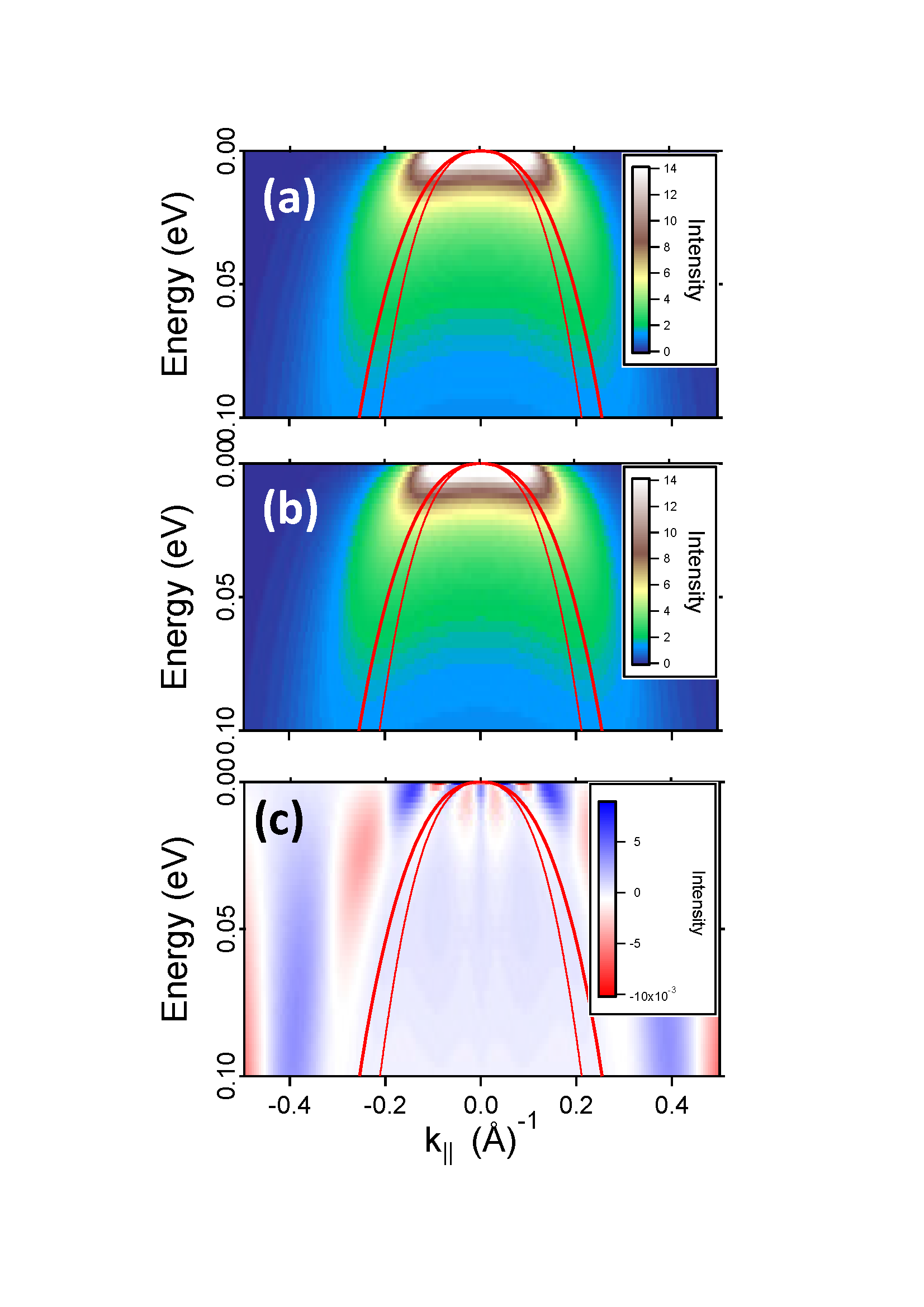
FIG. 1: (Color online) Spectral function for a marginal Fermi liquid with parameters given in the text. (a) calculated spectral function using Eq. (1). (b) Two-dimensional fit to the data in (a) using a variable renormalized dispersion and $\Im\Sigma$. (c) Difference between the calculated and the fitted spectral function. Note that the scale is reduced by a factor of 100 compared to (a) and (b). The solid red line depicts the fitted renormalized dispersion. The thin red line shows the dispersion derived from a fit of the MDCs with two Lorentzians.

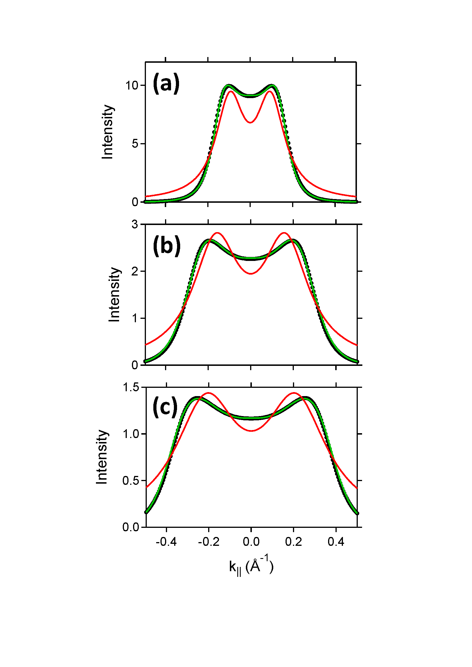
FIG. 2: (Color online) MDCs at various binding energies $E$. The black dots represent the calculated MDCs. The green curve is derived from the two dimensional fit of the spectral function. The red curve depicts a curve derived from a fit of a sum of two Lorentzians to the calculated spectral function. (a) $E=0.01$ meV. (b) $E=0.05$ eV. (c) $E=0.1$ eV.

In this section we develop a new method for the evaluation of the imaginary part of the self-energy for highly correlated systems and a non-linear dispersion. Furthermore we discuss the errors which may appear when the traditional methods are used. We propose to evaluate the measured spectrum by performing a two-dimensional fit using Eq (1). The fit parameters are the values of the imaginary part of the self-energy for the values of the binding energy used in the experiment and the renormalized dispersion as a function of energy $E$, approximated by a polynomial. The latter approximation is only useful for dispersions without kinks. In case of dispersions with kinks, a more complicated description of the dispersion is needed. Using the new method one can derive $\Im\Sigma$ also for highly correlated systems in which the spectral weight can no longer be separated into a coherent and an incoherent part. Moreover the method can also be applied for data in which a non-linear dispersion is detected. Furthermore this method can avoid the use of the not well defined bare particle dispersion, which is usually taken from DFT calculations.

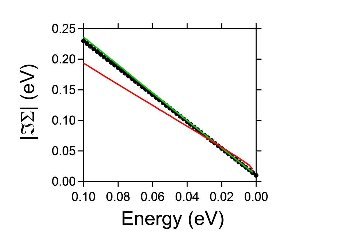
FIG. 3: (Color online) Black dots: calculated $\Im\Sigma$ using Eq. 3 with the parameters given in the text. Green line: $\Im\Sigma$ derived from the 2D fit to the calculated spectral function. Red line: $\Im\Sigma$ derived from the width of the Lorentzians multiplied by the velocity.

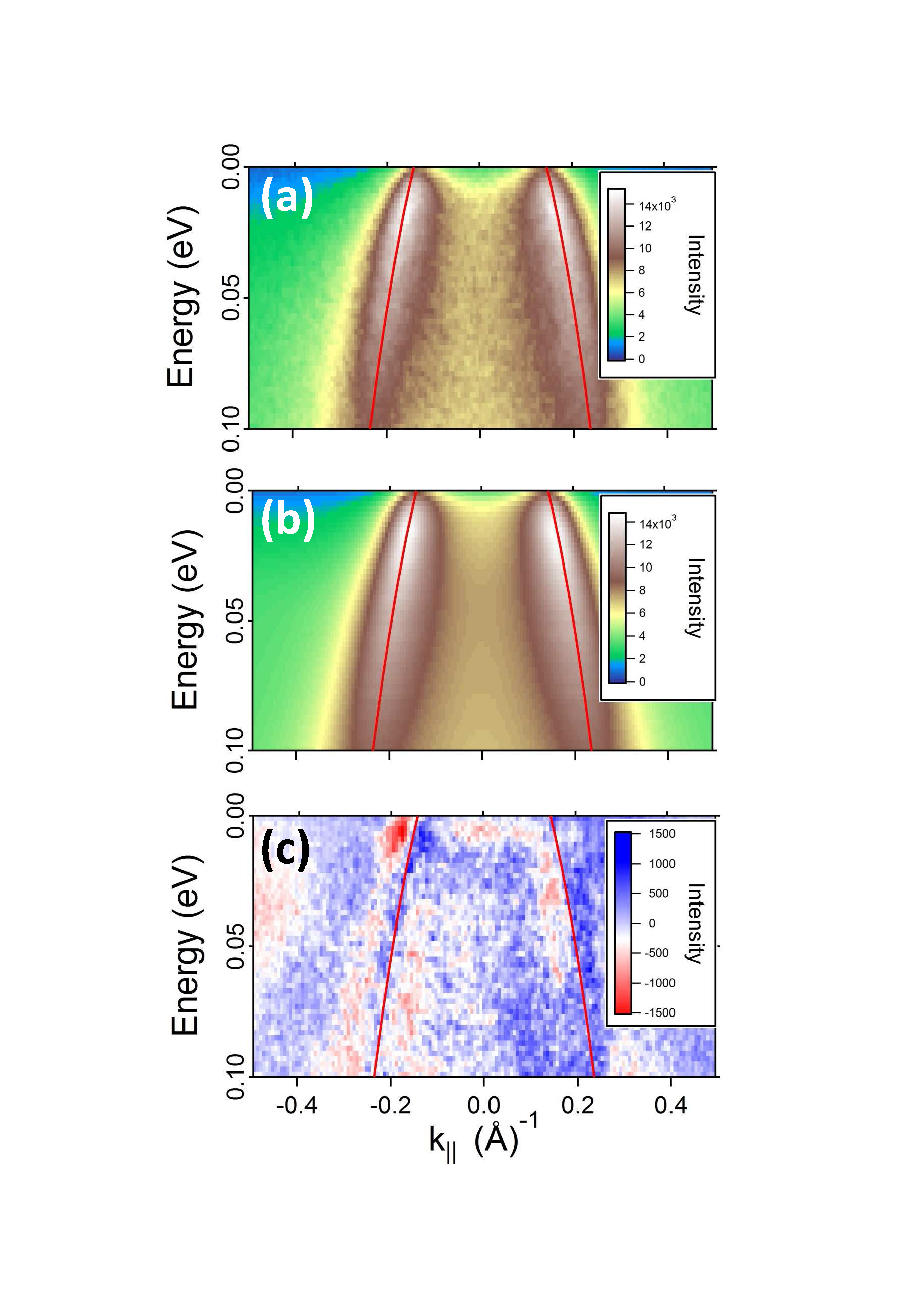
FIG. 4: (Color online) Analogous data as shown in Fig.1 but for real ARPES data of $\mathrm{K}_{x}\mathrm{Ba}_{1-x}\mathrm{Fe}_{2}\mathrm{As}_{2}$ .

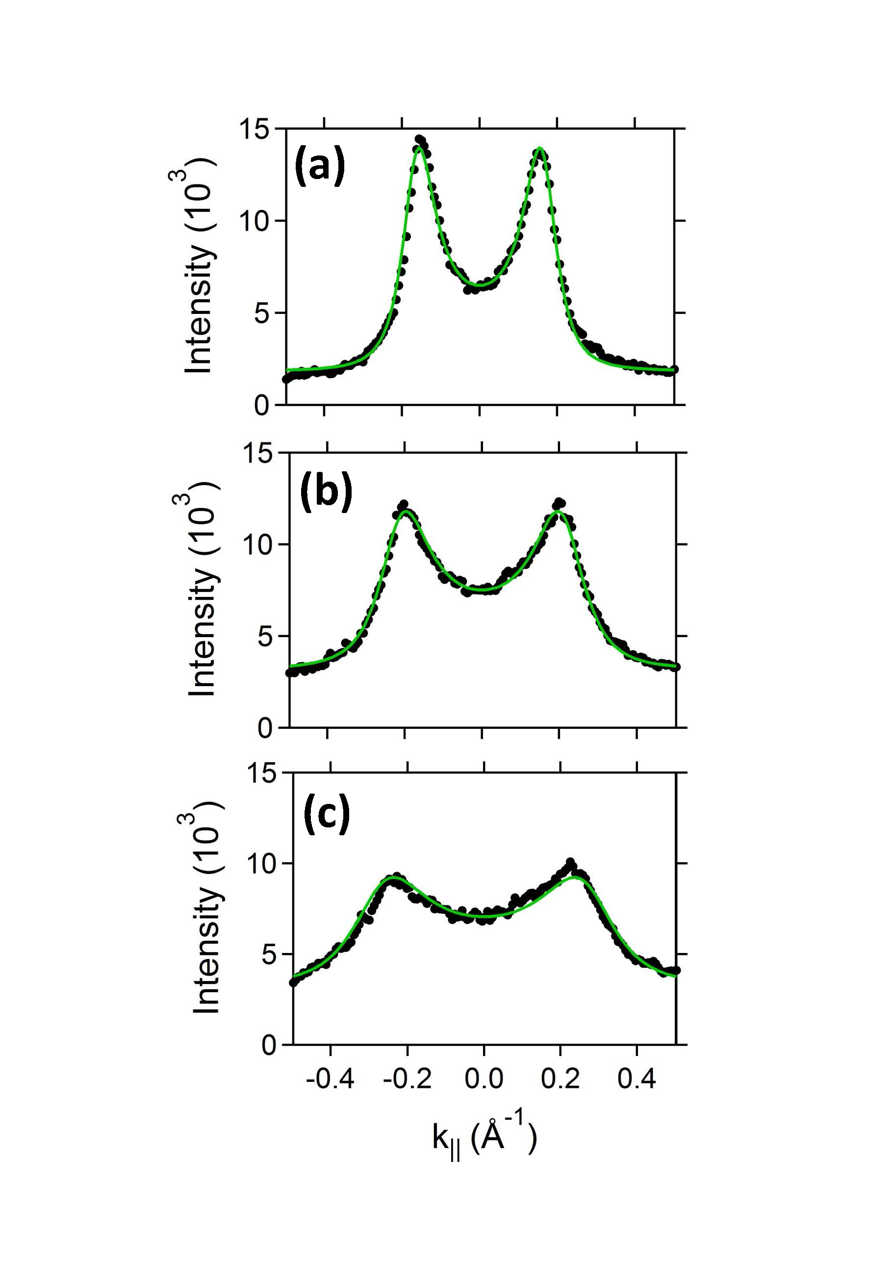
FIG. 5: (Color online) Analogous data as shown in Fig.2 but for real ARPES data of $\mathrm{K}_{x}\mathrm{Ba}_{1-x}\mathrm{Fe}_{2}\mathrm{As}_{2}$ $x=0.4$.

First we test the method using a calculated spectrum, using the self-energy function from a "marginal" Fermi liquid in which the coherent part of the spectral weight approaches zero ($Z=0$), a concept originally devised to phenomenologically describe the normal state of the cuprate superconductors. One assumes that the scattering rates at low energy are much higher compared to a normal Fermi liquid due to strong correlation effects and/or nesting. The self-energy is given by Varma2002

$$\Sigma=\frac{1}{2}\lambda_{MF}Eln\frac{E_{c}}{u}-i\frac{\pi}{2}\lambda_{MF}u,$$ (3)

where $u=max(|E|,kT)$, $kT$ is the thermal energy, $\lambda_{MF}$ is a coupling constant, and $E_{c}$ is an ultraviolet cutoff energy. At low temperatures the imaginary part of the self-energy is linear in energy. The $\Re\Sigma$ is no longer linear in energy as in a Fermi liquid and one has to solve Eq. (2) numerically to derive the dispersion. In the calculations we use the very high coupling constant $\lambda_{MF}=1.4$ corresponding to a slope $\beta=2.2$ of $\Im\Sigma(E)$ vs. $E$. The high coupling constant was used to demonstrate the difference between the new evaluation method and the standard evaluation method using the Lorentzian width and multiplying it with the renormalized velocity. In the calculation we also used a parabolic bare particle dispersion and a cutoff energy of $E_{c}=1.5$ eV. The calculated spectral function together with the dispersion derived from Eq. (2) and a dispersion derived from MDC fits with Lorentzians is shown in Fig. 1(a).

As shown previously Fink2015 for these high $\lambda$ values the renormalized dispersion at low energies is no longer parabolic due to the logarithmic term in Eq. (3). The spectral function derived from a 2D fit to the calculated spectral function is shown in Fig. 1(b). The difference between the calculated and the fitted spectral function is shown in Fig. 1(c).

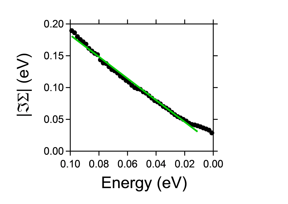
FIG. 6: (Color online) Analogous data as shown in Fig. 3 but for real ARPES data of $\mathrm{K}_{x}\mathrm{Ba}_{1-x}\mathrm{Fe}_{2}\mathrm{As}_{2}$ $x=0.4$.

As shown in Fig. 2 for various binding energies the MDCs of the calculated spectral function are no more a sum of two Lorentzians. Rather an asymmetric distribution determines the MDCs. An expansion of the dispersion about the $k_{M}$, the momentum at which the spectral function has a maximum, into a Taylor series and using a parabolic renormalized dispersion yields that the asymmetry is only zero when the renormalized velocity $v^{*}$ is much bigger than $\frac{\hbar}{m^{*}}\frac{W}{4}$. In addition one needs $\beta$ values which are much smaller than one to obtain a Lorentzian. Details of the new method will be published in a forthcoming publication. The derived deviations from a Lorentzian indicate that the standard evaluation of the lifetime broadening is not exactly working for data with a non-linear dispersion and/or with a slope of $\Im\Sigma$ which is not much smaller than one.

In Fig 3 we show $\Im\Sigma(E)$ calculated from Eq. (2), derived from the 2D fit, and derived from a fit of the MDCs by Lorentzians. While the 2D fit perfectly agrees with the calculated values, there is a difference of up to 17 % to the values derived from the fit with Lorentzians. The difference is reduced with increasing effective mass and decreasing coupling constant.

Next we illustrate the new method by showing the detailed evaluation of real ARPES data. We select the spectral function of the inner hole pocket of $\mathrm{K}_{x}\mathrm{Ba}_{1-x}\mathrm{Fe}_{2}\mathrm{As}_{2}$ $x=0.4$ shown in Fig. 1 of the main paper. In Fig. 4 we show the analogous data as in Fig. 1. In real ARPES data the amplitude of the spectral function is no more constant. Thus we have introduced an energy depending decrease of the amplitude in the fit, described by two fit parameters. Furthermore we have taken into account a k-independent background which slightly increases with increasing energy.

The fitted spectral function [see Fig 4(b)] is very close to the measured spectral function [see Fig 4(a)], which is also seen in the difference between the ARPES spectral function and the fitted spectral function [see Fig 4(c)]. The MDCs, presented in an analogous way as in Fig. 2 (see Fig. 5) are well described by the fitted MDCs. Finally, we present $\Im\Sigma$ derived from the fit in Fig. 6. Fitting the derived results by $\Im\Sigma=\alpha+\beta E$ yields $\alpha=0.01$ eV and $\beta=1.7$.

References

- (1) A. Damascelli, Z. Hussain, and Z.-X. Shen, Rev. Mod. Phys. 75, 473 (2003).
- (2) G. Mahan, Many-Particle Physics, Kluwer Academic, 2000.
- (3) C. Varma, Z. Nussinov, and W. van Saarloos, Physics Reports 361, 267 (2002).
- (4) J. Fink et al., Phys. Rev. B 92, 201106 (2015).