Thermodynamical String Fragmentation
Abstract
The observation of heavy-ion-like behaviour in pp collisions at the LHC suggests that more physics mechanisms are at play than traditionally assumed. The introduction e.g. of quark-gluon plasma or colour rope formation can describe several of the observations, but as of yet there is no established paradigm. In this article we study a few possible modifications to the Pythia event generator, which describes a wealth of data but fails for a number of recent observations. Firstly, we present a new model for generating the transverse momentum of hadrons during the string fragmentation process, inspired by thermodynamics, where heavier hadrons naturally are suppressed in rate but obtain a higher average transverse momentum. Secondly, close-packing of strings is taken into account by making the temperature or string tension environment-dependent. Thirdly, a simple model for hadron rescattering is added. The effect of these modifications is studied, individually and taken together, and compared with data mainly from the LHC. While some improvements can be noted, it turns out to be nontrivial to obtain effects as big as required, and further work is called for.
Keywords:
QCD Phenomenology, Phenomenological Models1 Introduction
QCD, the theory of strong interactions, is at the origin of a wide range of phenomena. In one extreme, progress on high-energy perturbative calculations offers an increasingly precise and successful description of hard processes, as a large community is steadily improving calculational techniques. NLO calculations, once rare, are now standard, NNLO is getting there, and even NNNLO is starting to appear (see e.g. Salam:2016lhcp and references therein). In another extreme, the nonperturbative aspects of low-energy interactions are less well understood. Lattice QCD can be used to calculate static hadron properties, but not (yet?) dynamical processes. Specifically, the description of hadronization, the step whereby partons turn into hadrons in high-energy collisions, cannot be derived directly from the QCD Lagrangian within any currently known formalism. Instead string Andersson:1983ia and cluster Field:1982dg ; Gottschalk:1983fm ; Webber:1983if models, developed in the early eighties, have been used almost unchanged from PETRA/LEP events to SS/Tevatron/LHC ones — the assumed ”jet universality”. Differences have been attributed to the quite disparate parton-level configurations that undergo hadronization: while involves only hard process and final-state radiation (FSR), pp adds aspects such as initial-state radiation (ISR), multiparton interactions (MPIs), beam remnants and colour reconnection (CR).
Cracks have started to appear in this picture as new LHC data have been presented. Specifically, several studies have shown how high-multiplicity pp events have properties similar to those observed in heavy-ion AA collisions. Some observations may have an explanation within the current framework, e.g. CR may give some flow-like patterns Ortiz:2013yxa , but others do not. An early example was the discovery of “the ridge”, an enhanced particle production around the azimuthal angle of a trigger jet, stretching away in (pseudo)rapidity Khachatryan:2010gv ; Aad:2015gqa ; Khachatryan:2016txc . A more recent example is the smoothly increasing fraction of strange baryon production with increasing charged multiplicity, a trend that lines up with pA data before levelling out at the AA results Adam:2016emw 111Note that in Cuautle:2016huw the authors obtain the same enhancement regardless of the system measured if the yield ratios are plotted against the estimated energy density.. Conventional wisdom holds that the formation of a quark–gluon plasma (QGP) requires a larger volume and longer time for thermalization than pp or pA systems can offer, so such trends are unexpected, see e.g. BraunMunzinger:2007zz .
It is therefore time to rethink the picture of hadronization in high-energy and high-multiplicity collisions. One possible approach is to imagine that a QGP is at least partly formed in pp collisions, such that individual colour fields (strings) cease to exist. Such a behaviour is already implemented in the EPOS model Pierog:2013ria . Another is to imagine that strings survive as a vehicle e.g. of short-range flavour correlations, but that their properties are modified. Colour ropes Biro:1984cf ; Bialas:1984ye ; Andersson:1991er is one such example, wherein several colour-triplet strings combine to a higher colour-representation field. A detailed implementation of rope dynamics is found in the DIPSY program Bierlich:2014xba . Both EPOS and DIPSY qualitatively describe several of the new key features, such as the increasing rate of strangeness production at higher multiplicities.
With the studies described in this article we want to add to the set of alternative models that can be used to compare with data. At best it may offer some new insights, at worst it will act as a straw man model. Firstly, rather than the particle-mass-independent Gaussian spectrum assumed in the standard string model, it introduces an exponential dependence, . This is split among possible flavours according to hadronic , . Such and shapes were used to describe early pp data, e.g. at the ISR Capiluppi:1973fz , and has some foundation in the Hagedorn temperature Hagedorn:1965st ; Hagedorn:1970gh ; Hagedorn:1983wk and in related Barshay:1972jy ideas. (Later powerlike ansätze Hagedorn:1983wk ; Tsallis:1987eu ; Cleymans:2016opp or two-component exponential + powerlike ones Bylinkin:2012bz can be viewed as a consequence of perturbative jet production, and is in our framework generated as such, in an earlier stage than the nonperturbative hadronization.) Secondly, it assumes that the close-packing of several strings leads to an increased effective temperature and thereby both a changed particle composition and changed spectra. In spirit this is close to the rope model, but it does not have to assume that the individual strings either fuse or melt away. Thirdly, if the fragmenting strings are close-packed this also implies the initial formation of a dense hadronic gas, wherein rescattering may lead to collective-flow effects. Such effects are simulated in a crude first approximation.
The impact of these mechanisms on experimental distributions is studied, in order to quantify their significance. As a prime example, consider the distribution, with a characteristic rising trend that has been proposed as a signal for colour reconnection Sjostrand:1987su . Alternative interpretations are now offered in terms of close-packing of strings and/or hadrons, and these are presented and compared with data individually. At the end of the day, we should expect the “true” nature of high-multiplicity collisions to contain many contributing mechanisms, however. To be more more specific, in quantum mechanics any process that is not explicitly forbidden by some selection rule is bound to occur, the question is only with what rate. The final task therefore is try to constrain the relative importance of the mechanisms, not to prove a specific one “right” or “wrong”.
The new model components are implemented as options in the standard Pythia event generator Sjostrand:2006za ; Sjostrand:2014zea , which makes it easily accessible for further experimental tests. They should be viewed as a first iteration. Should they prove useful there is room for further improvements, as we will indicate.
The article is organized as follows. Section 2 outlines relevant features of the existing Lund string model and introduces key observables, with emphasis on those new ones that are not well described by the current Pythia generator. Section 3 introduces the alternative approaches explored in this article, and presents some first toy studies for simplified string topologies. Comparisons with data are presented in section 4, highlighting what seems to work where and what not. Finally section 5 contains a summary and outlook.
2 Existing Models and Data
2.1 The Lund string model
The Lund string fragmentation model Andersson:1983ia is very successful in many respects, but more so for the overall longitudinal fragmentation structure than for its description of the particle composition.
The central assumption in the string model is that of linear confinement, , with a string tension GeV/fm. The word “string” should here not be taken literally; the physical object is a kind of flux tube stretched between the endpoints, with a typical transverse size of the order of the proton one, fm. The one-dimensional “mathematical” string should then be viewed as a description of the location of the center of the flux tube. By analogy with superconductivity the tube could be viewed as a vortex line like in a type II superconductor, alternatively as an elongated bag in a type I one.
In the case of a simple stable back-to-back system, with , quarks move with the speed of light in “yo-yo”-mode oscillations, as energy moves between being stored in the endpoint quarks and in the intermediate string. If creation of new pairs is allowed the original system can break up into smaller ones, each a colour singlet in its own right. Denoting the original pair , and ordering the new pairs from the quark end, results in the production of hadrons , , …, .
Aligning the axis with the string axis, the breakup vertices are characterized by their location . These vertices have a spacelike separation, and so have no unique time ordering. (Except for the original of course. But here it is actually the turning points of the and that define the vertices in eq. (1) below, and then spacelike separation is restored.) Two adjacent ones are correlated by the constraint that the hadron produced should have the correct mass :
| (1) |
If the vertices are assigned from the quark end, say, each new vertex therefore corresponds to one degree of freedom, which should be selected according to some probability function. Imposing consistency constraints, mainly that results should be the same (on the average) if fragmentation is instead considered from the antiquark end, gives the solution Andersson:1983ia
| (2) |
with and two free parameters, and where once transverse momentum is introduced. Here is the fraction of available lightcone momentum taken by a hadron, with the remainder retained by the string for subsequent particle production.
This ansatz leads to vertices having an equilibrium distribution (after having taken a few steps away from the endpoints)
| (3) |
with the same and as above. (For the special case this result agrees with the Artru-Mennessier model Artru:1974hr , which is based on constant decay probability per string area , without any mass constraint.) The associated probability for producing particles can be written as Andersson:1985qr
| (4) |
where is the total space–time area under the breakup vertices. The relation between and (at a reduced c.m. energy) is then given by the fragmentation function eq. (2), where it is easy to show that the exponentials match, and somewhat less trivial that a larger (i.e. larger weight for higher multiplicities) corresponds to a larger (i.e. less momentum taken away in each step).
The simple fragmentation picture can be extended to topologies if the gluon is viewed as having separate colour and anticolour indices, as in the limit 'tHooft:1973jz . Then one string piece is stretched between the quark and the gluon, and another between the gluon and the antiquark. The absence of a string piece stretched directly between the quark and antiquark leads to predicted asymmetries in the particle production Andersson:1980vk that rapidly were observed experimentally Bartel:1981kh . In general, a string can stretch from a quark end via a number of intermediate gluons to an antiquark end. Technically the motion and fragmentation of such a string system can become rather complicated Sjostrand:1984ic , but the fragmentation can be described without the introduction of any new principles or parameters. This is the most powerful and beautiful aspect of the string fragmentation framework. Note that the leading hadron in a gluon jet can take momentum from both the string pieces that attaches it to colour-adjacent partons. This is unlike cluster models, where gluons are forced to branch into pairs, such that smaller colour singlets are formed rather than one single string winding its way between the partons. The string model is easily extended to closed gluon loops and, with rather more effort Sjostrand:2002ip , to junction topologies, where three string pieces come together in a single vertex.
We now turn to the breakup mechanism. If a pair is massless and has no transverse momentum it can be produced on-shell, in a single vertex, and then the and can move apart, splitting the string into two in the process. But if the (and ) transverse mass this is no longer possible. By local flavour conservation the pair is still produced at a common vertex, but as virtual particles that each needs to tunnel out a distance . Using the WKB approximation Andersson:1983ia to calculate the tunneling probability for the pair gives a factor
| (5) |
where the Gaussian answer allows a convenient separation of the and dependencies (with implicit phase space ).
The latter is implemented by giving the and opposite and compensating kicks, with . A hadron receives its as the vector sum of it and constituent kicks, and thus . Empirically the tuned value comes out larger than this, actually closer to GeV. This implies that almost half of the kick is coming from other sources than tunneling. One source could be soft gluon radiation below the perturbative (parton shower) cutoff, where becomes so big that perturbation theory breaks down Andersson:1981xu . Effectively radiation near the perturbative/nonperturbative border is thus shoved into an artificially enhanced tunneling answer, with the further assumption that the Gaussian shape and the balancing inside each new pair still holds.
Uncertainties also arise in the interpretation of the mass suppression factor of eq. (5): what quark masses to use? If current quark masses then the and ones are negligible while the is below 0.2 GeV, predicting less strangeness suppression than observed, while with constituent masses GeV and GeV Close:1979bt too much suppression is predicted. Intermediate masses and suppression factors closer to data can be motivated e.g. by noting that an expanding string corresponds to confinement in the two transverse dimensions but not in the longitudinal one. In the end, however, the suppression is viewed as an empirical number to be tuned to data. Whichever values are used, and quark tunneling production is strongly suppressed, so this mechanism can be totally neglected relative to the perturbative ones.
Considering only mesons in radial and rotational ground states, i.e. only the pseudoscalar and vector multiplets, naive spin counting predicts relative rates , whereas data prefers values closer to , at least for . It is possible to explain a suppression of the vector mesons based on the difference in the hadronic wave functions, from the spin–spin interaction term Andersson:1983ia , but the amount has to be tuned to data. And further brute-force suppression factors are needed specifically for the and mesons, which have “unnaturally” large masses owing to the anomaly.
Baryon production can be introduced by allowing diquark–antidiquark breakups of the string Andersson:1981ce , to be viewed as occurring in two consecutive creation steps Andersson:1984af . A baryon and the matching antibaryon would normally be nearest neighbours along the string, but the “popcorn mechanism” also allows one (or more) mesons to be produced in between. Diquark masses can be used to derive approximate suppressions, but again free parameters are used, for , , and others. Unfortunately the tuned values do not always match so well with the tunneling-formula expectations.
In total parameters are used to describe the outcome of the string/tunneling mechanism for particle production. Notable is that the particle masses do not enter explicitly in these considerations. This is unlike cluster models, e.g., where hadron masses occur in the phase space available for different cluster decay channels. A fair overall description of the particle composition is then obtained with very few parameters Platzer:2011bc ; Richardson:2012bn . Note that while most fragmentation parameters in Herwig++ exist in different copies for light , , and quarks, the ones for heavy quarks have either been set equal to the values of those for light quarks Platzer:2011bc or have not been included in further tuning processes Richardson:2012bn .
The hadron masses can be explicitly introduced into the Lund framework by assuming that the integral , with given by eq. (2), provides the relative normalization of possible particle states. This concept has been developed successfully within the UCLA model Chun:1997bh ; Abachi:2006qf , in that particle rates come out quite reasonably with minimal further assumptions. There are some other issues with this approach, however, and we do not pursue it further here.
2.2 Key data
An immense number of studies have been published based on hadron collider data, and it is not the intention here to survey all of that. Instead we here bring up some of the key data and distributions that have prompted us to this study. Several of them will be shown repeatedly in the following. We note that all histograms we will present in this article are produced by utilizing Rivet Buckley:2010ar .
The list of key observables includes:
-
•
The change of flavour composition with event multiplicity. Specifically, high-multiplicity events have a higher fraction of heavier particles, meaning particles with a higher strangeness content Adam:2016emw . Pythia contains no mechanism to generate such a behaviour. On the contrary, within a single fixed-energy string a higher multiplicity means more lighter particles, for phase space reasons. In collisions a higher multiplicity is predominantly obtained by more MPIs, however, so the composition stays rather constant.
-
•
The average transverse momentum is larger for heavier particles, both at RHIC Abelev:2008ab and LHC Abelev:2014qqa . This is a behaviour that is present also in Pythia, and comes about quite naturally e.g. by lighter particles more often being decay products, with characteristic values smaller than the primary particles in the string fragmentation. The mass dependence is underestimated, however. That is, obtains a too large in Pythia and baryons a too small one. Recently has also been presented as a function of , inclusive Aad:2010ac and for different hadron species Bianchi:2016szl , providing a more differential information on this mismatch. In figure 1 we show these observables and compare default Pythia with data, with the above expected conclusions. Note that the data in figure 1 of Bianchi:2016szl is not (yet) publicly available. To obtain an estimate of the data that is comparable to MC predictions we used an estimate of the logarithmic fits shown in figure 1 of Bianchi:2016szl and used values on the axis rather than .
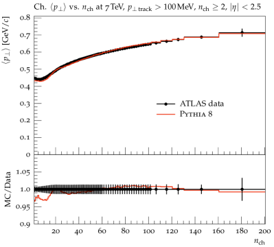
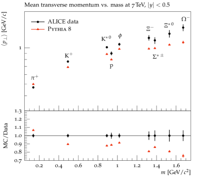


Figure 1: The mean transverse momentum as a function of the charged multiplicity (top left and the hadron mass (top right) and bottom). Predictions of default Pythia compared to ALICE Bianchi:2016szl ; Abelev:2014qqa and ATLAS Aad:2010ac data. The data in the bottom plots is taken to be an estimate of the logarithmic fits in Bianchi:2016szl and therefore no error bars are included. -
•
The charged particle spectrum is not correctly modelled at low scales, with Pythia producing too few particles at very low values Aad:2010ac ; Chatrchyan:2011av ; Adam:2015pza . Often tunes then compensate by producing a bit too many at intermediate scales. The issue shows up e.g. in minimum-bias distributions, where it is not possible to obtain a good description for data analyzed with GeV and GeV simultaneously.
-
•
In the spectra for identified particles Adam:2015qaa it turns out that the deficit at low is from too little production. This is not unexpected, given the previous two points, but stresses the need to revise the mass dependence of spectra.
-
•
The spectrum ratio, measured by CMS Khachatryan:2011tm , where Pythia is not able to reproduce the peak at GeV completely and overshoots the distribution for large- values.
-
•
The observation of a ridge in collisions was one of the major surprises in the 7 TeV data Khachatryan:2010gv , and has been reconfirmed in the 13 TeV one Aad:2015gqa ; Khachatryan:2016txc . The ridge is most clearly visible at the very highest multiplicities, but more careful analyses hints the effect is there, to a smaller extent, also at lower multiplicities. Like in heavy-ion collisions one may also seek a description in terms of correlation functions, , notably the coefficient, with a similar message. These phenomena are not at all described by Pythia: there is no mechanism that produces a ridge and, once the effects of back-to-back jet production have been subtracted, also no rise of .
There are also some other reference distributions that have to be checked. These are ones that already are reasonably well described, but that inevitably would be affected by the introduction of new mechanisms.
-
•
The charged particle multiplicity distribution is sensitive to all mechanisms in minimum-bias physics, but especially the MPI and CR modelling. A mismatch in is most easily compensated by modifying the scale of the MPI description. This parameter is used to tame the divergence of the QCD cross section to a finite shape. It can be viewed as the the inverse of the typical colour screening distance inside the proton. A mismatch in the width of the distribution can be compensated by a modified shape of the impact-parameter distribution of the two colliding protons. Specifically, a distribution more sharply peaked at gives a longer tail towards high multiplicities.
-
•
An increasing with was noted already by UA1 Albajar:1989an , and has remained at higher energies Aad:2010ac ; Bianchi:2016szl . It offers a key argument for introducing CR in collisions, as follows Sjostrand:1987su . The tail towards large is driven by events with more MPI activity, rather than e.g. by events with higher- jets. If each MPI subcollision produces particles essentially independently the would be rather flat. CR implies that fewer and fewer extra particles are produced for each further MPI, as the possibilities to reduce the total string length by CR increase the more partons are already present. The amount of from the MPIs thus increases faster than the , meaning more per particle. (To this comes the normal hadronization contribution, which raises the overall level but does not contribute to the slope.) The exact nature of CR is not known, meaning that many models have been developed Sjostrand:1987su ; Sjostrand:1993hi ; Christiansen:2015yqa . In most of them there is some overall CR strength parameter that can be adjusted to fit the slope.
-
•
A natural reference for hadronization properties always is data. The principle of jet universality — or, in our case, string universality — is deeply rooted, so it it useful to check that no changes of fundamental string properties have too adverse an impact on . There is also a possibility of improvements in some places, like the inclusive and spectra; unfortunately these are not available for identified particles.
3 The New Models
In this section we outline the basic ideas and implementations that we have developed to offer new options to the traditional Pythia hadronization framework. As we later compare with data we will have reason to go into more detail and discuss some variations.
3.1 Variations of the normal string model
As described above, the standard tunneling framework suggests a Gaussian suppression of the production of heavier quarks and diquarks, with a further suppression based on the hadronic spin state, but no obvious room for an explicit dependence on the hadron mass. It also provides a common Gaussian spectrum for all new pairs. We will study a few variations of this framework, mainly as a reference for the thermodynamical ansatz below.
Firstly, consider a Gaussian suppression associated with the masses of the produced hadrons rather than with the quarks. That is, let the relative production rate of different hadron species be given by a factor , which factorizes into a species-independent spectrum and an mass suppression. The question is then whether this would give the appropriate suppression for the production of heavier particles.
Secondly, the universal spectrum could be broken by assigning a larger width in string breakups of the and kinds, relative to the baseline and ones. The issue to understand here is how dramatic differences are required to get a better description of the individual , and spectra.
Thirdly, assume that more MPIs leads to a closer packing of strings in the event, but that each string “flux tube” remains as a separate entity. The transverse region of the string shrinks and, essentially by Heisenberg’s uncertainty relations, this should correspond to a higher energy, i.e. a larger string tension . (Such a relation comes out naturally e.g. for bag models of confinement Chodos:1974je .) Overall the dense-packing effect on and related parameters should scale as some power of , i.e. the number of MPIs in the current event. Since and are strongly correlated it is thus interesting to study how the particle composition and depend on . For a more differential picture it should be preferable to estimate the number of strings in the neighbourhood of each new hadron being produced.
This is done by making a reasonable guess for the momentum of the hadron that is the next to be produced on the current string. Using an average hadron mass and , defined in the frame of the parent string, and an average value of , the momentum of the “average expected” hadron is calculated. Using this information, we determine the number of strings that cross the rapidity of the expected hadron. For this purpose the rapidity range that a string will populate is defined by the rapidity of the endpoint partons of each string piece,
| (6) |
where has the purpose to protect against strings with low- endpoints from populating the full rapidity range. The rapidity-density measure is reasonable for low- hadroproduction, but does not reflect the phase space inside a high- jet, where close-packing of strings should be rare. Therefore the effective number of strings is calculated as
| (7) |
where is the physical hadron and is the MPI regularization parameter.
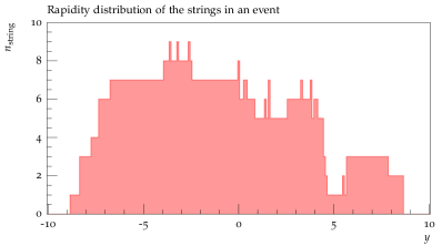
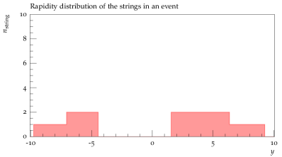
As two examples, the rapidity distribution of the strings in a typical QCD event and in a diffractive event are shown in figure 2. Using eq. (7), the string tension in eq. (5) is modified to be
| (8) |
where the exponent is a left as a free parameter, that can be used to tune the model to data. Note that while junctions222A junction topology corresponds to an Y arrangement of strings, i.e. where three string pieces have to be joined up in a common vertex. contribute to the calculation of by assuming one string stretched between the highest- and lowest-rapidity parton, their fragmentation does not make use of eq. (8). Junctions are rare in the models we study, so this is not a significant simplification.
The effect of modifying the string tension due to the local density has also been studied in other Monte Carlo programs, which are primarily for heavy-ion collisions. Some of them have hardly been used for pp physics as they miss out on other physics aspects such as QCD jet production. In the RQMD model Sorge:1989dy for studying relativistic nucleus-nucleus collisions, colour strings are allowed to fuse into ropes if they are overlapping, which weakens the suppression of strangeness and baryon production due to the increased string tension Sorge:1992ej . A similar model with string fusion into colour ropes is implemented in the DIPSY event generator Bierlich:2014xba and shows improvement in the description of identified particle spectra in pp minimum bias data. For the UrQMD model Bass:1998ca ; Bleicher:1999xi , used for relativistic heavy-ion and hadron-hadron collisions, the authors of Soff:2000ae show that a better description of particle yields is achieved with an enhanced string tension. The effect of an increased string tension in a densely populated environment on strangeness and diquark production, antibaryon-to-baryon ratios and other observables has been investigated in Soff:2002bn . In AMPT Zhang:1999bd ; Lin:2004en , a Monte Carlo transport model for heavy-ion collisions at relativistic energies, parameters in the Lund string fragmentation model have been modified, as the string tension is expected to be increased in the dense matter formed in heavy-ion collisions Lin:2000cx . In the PSM Amelin:1993cs ; Amelin:2001sk Monte Carlo model for simulating nuclear collisions, string fusion associated with high string densities is taken into account to reduce multiplicities and increase , baryon and strangeness production. Ref. Braun:1992ss presents a model which introduces the interaction between strings via their fusion and percolation analytically. The of the produced particles, and therefore also the string tension, depends on the string density and how much strings overlap Braun:1999hv ; Braun:2000hd ; Pajares:2005kk .
3.1.1 One-string toy model
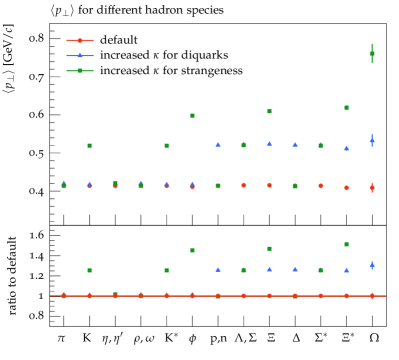
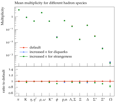
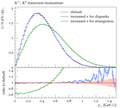
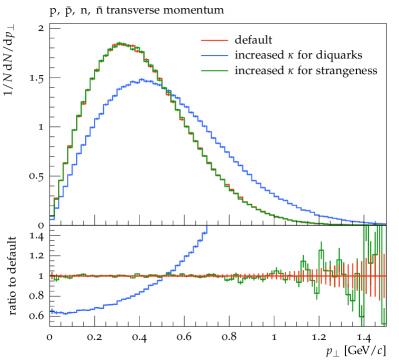
A very simple toy model is introduced to validate the modifications to the string tension in the conventional string model. A single string with energy is spanned along the axis. The flavour of the endpoint quarks is chosen random from the set . The study includes only primary produced hadrons, i.e. no hadron decays, and also excludes the hadrons containing the endpoint quarks. (Such hadrons would have lower since the endpoint quarks by definition have .)
The and the mean multiplicity for different hadron species are shown in figure 3. As expected, increasing the string tension either for quarks or for diquarks leads to an increased value for the hadrons concerned. Note that for the is only increased slightly due to the quark component being more frequently produced compared to . There is a slight reduction of the production probability for hadrons with quarks or diquarks, shown in the top right plot in figure 3, due to the increased string tension leading to fewer particles being produced in affected events. The bottom row of figure 3 shows the and spectra, shifted to larger values as the string tension for that hadron species is increased.
3.1.2 Multi-string toy model
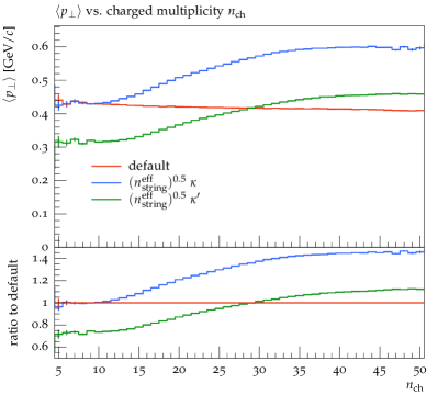
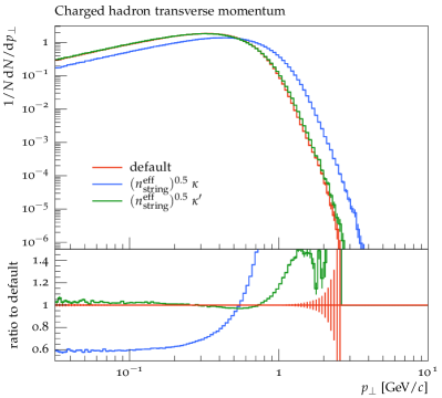
To investigate the effect of the close-packing of strings, as in eq. (8), the above toy model is extended to include several strings along the axis. The number of strings is picked randomly between two and eight and the string energies are chosen such that they sum up to . Figure 4 shows as a function of the number of charged particles and the distribution and compares the modified model to default Pythia. Two different choices for the baseline value for the string tension are made in case of taking the close-packing of strings into account. In the first case the tension is denoted with and its value is adjusted such that agrees with default Pythia for small values of . In the second case, where the string tension is denoted by the value is adjusted to obtain the same , averaged over all hadrons and charged multiplicities. The latter case serves as a cross check when investigating the influence on the spectrum of charged hadrons.
As expected the increases with the charged multiplicity, eventually flattening out at large multiplicities. The left histogram in figure 4 also nicely shows that the rise is independent of the baseline string tension value.
When fitting the string tension such that the same overall is reached as in the default model, the charged hadron spectrum exhibits only small changes; making the spectrum somewhat broader.
3.1.3 Gaussian suppression
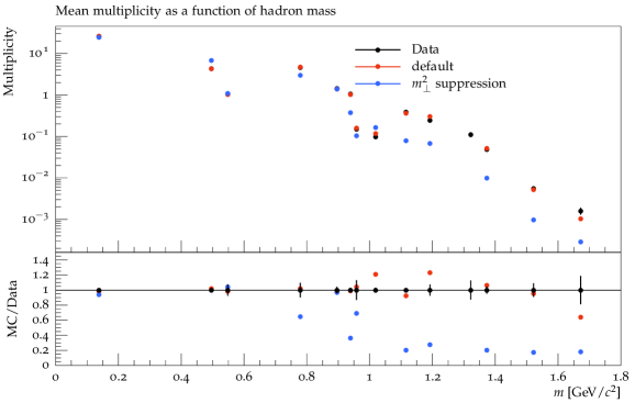
To test the applicability of the Gaussian transverse mass suppression, the quark is generated according to , see eq. (5), with the hadron flavour chosen based on . The additional factor of two arises from the hadron receiving contributions from two quarks. As the comparison to data is of interest here, realistic events with are investigated. In figure 5 the particle composition is shown as a function of mass. This clearly indicates that the suppression based on the transverse mass squared of the hadrons is suppressing heavier hadrons too much. We will therefore not consider this option further.
3.2 The thermodynamical string model
The most radical departure from standard Lund string principles that we explore in this article is to replace the Gaussian suppression factor in mass and by an exponential one. To be more explicit, instead of a quark-level suppression governed by eq. (5) there will be a hadron-level suppression
| (9) |
The inspiration clearly comes from a thermodynamical point of view, which is why we choose to associate the dimensional parameter with a temperature . This association should not be taken too literally, however; there are many differences relative to a purely thermal model. The main one is that we keep the longitudinal string fragmentation structure unchanged, which ensures local flavour conservation. Another is that e.g. the Hagedorn approach Hagedorn:1965st ; Hagedorn:1970gh is based on the assumption of a steeply increasing density of excited states as a function of mass, whereas we only include a few of the lowest multiplets. (By default only the ground states corresponding to no radial or orbital excitation, optionally also the lowest meson multiplets.) This means that, although our comes out to be a number of the order of the Hagedorn temperature, there is no exact correspondence between the two. Also, from dimensional considerations, so our could be viewed as a manifestation of the string energy per unit length, not directly linked to a temperature.
There is also an experimental historical background to the choice of an exponential shape, in that already fixed-target and ISR data showed that a distribution like offered a good fit to the inclusive spectrum, with Capiluppi:1973fz ; Alper:1975jm ; Guettler:1976fc ; Giacomelli:1979nu . With data split by particle type, a lower value is noted for kaons and protons than for pions, but with the modified form all the spectra can be described by almost the same value.
As an aside, the preference for an exponential shape was and is not a show-stopper for the Gaussian approach in the normal string fragmentation. At larger the spectrum is dominated by the fragmentation of (mini)jets, giving a larger rate than the nonperturbative hadronization one. And at smaller the pattern of decays makes the spectrum more steep than the Gaussian one of the primary hadrons. So at the end of the day a Gaussian ansatz lands not that far away from an exponential spectrum, although differences remain. See further section 3.4.1, in particular figure 9.
In more detail, our model is intended to give each new hadron in the string fragmentation a according to an exponential distribution. We want to preserve the concept of local conservation in each breakup vertex, so seek a distribution that convoluted with itself (in two transverse dimensions) gives an exponential,
| (10) |
Using Fourier transforms to turn the convolution into a product,
| (11) |
The transformation back of then gives Gradshteyn:1980
| (12) |
where , is a regular Bessel function of the first kind, and is the modified Bessel function of the second kind of order . An implementation of has been included in Pythia based on Abramowitz:1965 , using a power series for and an asymptotic expansion for .
Consider the fragmentation of a string, where the quark of one breakup has a certain . The transverse momentum of the (di)quark of the next breakup pair is constructed by picking its absolute value according to eq. (12) and a random azimuthal angle. The partner anti(di)quark must thus have due to local momentum conservation. The hadron transverse momentum is simply the sum of the of the two contributing quarks, . Having at hand we decide on the flavour of the breakup pair , and therefore also on the hadron species, as follows: calculate the transverse mass of all hadrons whose flavour content includes the incoming quark and determine the basic probability for each hadron as
| (13) |
Assuming the production of two hadrons with different masses and , then eq. (13) implies the same production rate for , but more suppression of the heavier hadron at low . Thus there is less production of heavier states, but they come with a larger .
As mentioned above, by default we only include the light-flavour meson and baryon multiplets without radial or orbital excitation 333Heavy flavour hadrons are of course included to handle the endpoint quarks of the strings, where needed.. However, if desired, more hadrons can be added to the procedure. Depending on the flavour content of the hadron, the probability in eq. (13) receives additional multiplicative factors:
-
Due to spin-counting arguments vector mesons receive a factor of and tensor mesons a factor of .
-
For same-flavour mesons we include the diagonal meson mixing factors, similar to what has been done previously in the conventional Lund string model.
-
Baryons receive a free overall normalization factor with respect to mesons, as well as an additional factor stemming from the symmetry factors, see Andersson:1981ce . The relative weight of spin baryons with respect to those with spin is , similar to the factors for mesons arising from the spin-counting arguments in point 1.
-
For the special case of octet baryons with three different flavours, e.g. and , their probability for different internal spin configurations is taken into account.
-
An extra suppression factor for hadrons with strange (di)quarks is included to get more control over the relative hadron production and thus a better description of data.
All probabilities are then rescaled to sum up to unity and the hadron species and therefore the flavour of the next (di)quark pair is chosen accordingly. Note that we have not (yet) implemented popcorn baryon production, i.e. no mesons are produced in between a baryon and its antibaryon partner.
Similar to eq. (8) the temperature can be modified as
| (14) |
with given in eq. (7) to take into account the effect of close-packed strings. Note that in DiasdeDeus:2006xk the temperature has been related to the density in the context of the percolation of color sources (the density is however defined differently).
3.2.1 Asymmetry in different flavour transitions
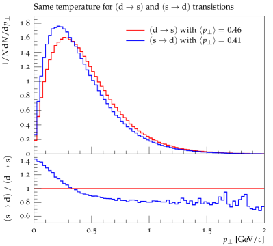
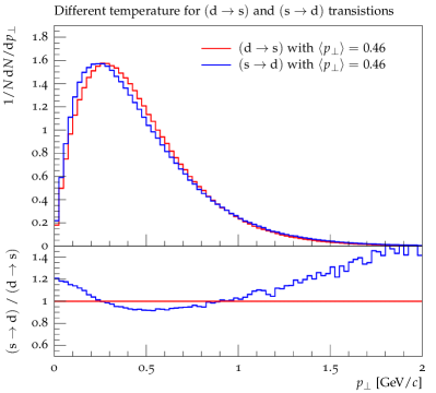
Consider a very simple model, where only string breaks with and quark pairs are allowed to produce only pseudoscalar mesons, and the mixing of diagonal mesons is ignored. Then it is rather easy to see that the spectra and of the hadrons produced in transitions is not the same as for transitions, due to the difference in competition. In the first instance competes with , and since the former produces the heavier meson it also obtains the higher . In the latter instance instead competes with and so gives the lighter meson and lower . Assuming that fragmentation is performed from the quark end inwards, would thus obtain a harder spectrum than , which should not be the case. A simple solution for obtaining the same for both and transitions is to adjust the temperature in eq. (13) in case of initial quarks such that and hadrons are produced with the same value, higher than , and becomes even higher than that.
In figure 6 we show the spectra for both types of transitions with the same temperature and with the adjusted temperature. Note that though both transitions end up with the same value, the shape of the distribution still differs somewhat.
Unfortunately this is a price to pay for working with a recursive model, where flavour is conserved locally. A traditional thermal model based on eq. (13) would not conserve flavour or momentum, however, so is not an option here.
3.3 The hadronic rescattering model
A close-packing of fragmenting strings also implies a close-packing of the produced primary hadrons, i.e. a dense hadronic gas. This gives the possibility for hadrons to rescatter on the way out, in particular at the earliest times after hadronization. A detailed simulation of this mechanism would require a knowledge of where in space–time each hadron is produced. For a single string, say stretched along the axis, it is straightforward to translate between the values of the primary hadrons and the coordinates of the string breakups. For the more realistic case, when a string is stretched between several partons and the string motion is considerably more complicated Sjostrand:1984ic , appropriate rules have not been worked out. To this should be added ambiguities in the transverse production coordinates, both as a consequence of the transverse distribution of the MPIs and of transverse fluctuations inside each string. The modelling of all of these aspects is an interesting task for the future. In addition, the cross section for the scattering of two hadrons against each other varies between hadron kinds, and depends on the relative energy of the two, adding a further layer of complexity.
Here we want to avoid such a detailed model, but still be able to explore whether hadronic rescattering effects could contribute to the resolution of some of the effects that we are attempting to explain. Collective flow — whether dictated by properties of the QGP or by hadronic rescattering — is well-established in heavy-ion collisions, see e.g. Gyulassy:2004zy ; Heinz:2013th ; Roland:2014jsa and references therein. In particular, a common average radial velocity means that heavier particles have a higher than lighter. Of course we do not expect as dramatic effects in , but they may still contribute to the same kind of separation as in the thermodynamic scenario above, so it should be interesting to compare the two possibilities.
The simple modelling we have in mind is applied to the primary hadrons produced directly from the string fragmentation, before secondary decays are considered. Furthermore, for strings stretched along the axis there is a strong correlation between the rapidity of a particle and its space–time production vertex. Therefore, for a given hadron, the density of other hadrons at around the same rapidity is a reasonable (and longitudinally boost invariant) measure of how close-packed particle production is. If there is a contribution from particles coming from the same simple string it has presumably already been absorbed in the tuned fragmentation parameters, so we should disregard such pairs. Unlike events, however, it is common with topologies where a string consists of pieces stretched back and forth across the same rapidity range, and then the above argument does not apply. In practice, it is therefore more relevant to exclude rescattering only between close neighbours in the fragmentation chains.
One should further note that the rapidity density of hadrons refers to low- particles. The hadronization of a scattered high- parton mainly occurs at larger scales, and these hadrons would be essentially unaffected.
The angular distribution of a rescattering, defined in the rest frame of the hadronic pair, should depend on the orbital angular momentum . For simplicity, we restrict to -wave isotropic scattering (i.e., ) by requiring that the classical value of angular momentum , where is the impact parameter and is the maximally allowed three-momentum of the hadrons in their rest frame, left as a (in principle) free parameter. We don’t have access to for each pair, but assume it is the same distribution for all combinations of hadron types. A common restriction on the three-momentum is thus introduced for all pairs, which is implemented as a cut on the invariant mass of the hadron pair,
| (15) |
with and being the masses of the hadrons and the physical invariant mass of the hadron pair. For all hadron pairs that are not excluded by eq. (15) we calculate the difference in rapidity, , and the rescattering probability. For hadrons that are not produced in the same string the latter is
| (16) |
where the maximum scattering probability and the maximum rapidity difference are left as free parameters. Eq. (16) simply means a probability of for zero rapidity difference of the hadron pair, linearly decreasing to zero at a rapidity difference of .
As an alternative to eq. (16), without the cut on the invariant mass in eq. (15), the probability can be chosen to be
| (17) |
with being the difference in azimuth of the hadron pair and the maximally allowed value of the radius .
For hadron pairs that are produced in the same string we introduce the difference in hadron index (called rank e.g. in Field:1977fa ), , to denote how close two hadrons are, i.e. two neighbours have , next-to-neighbours and so on. The scattering probability for same-string hadrons is
| (18) |
where is the minimum/maximum probability associated with the nearest/furthest neighbour, characterized by , with a linear behaviour of the probability in between; zero probability for hadrons closer than and maximum probability for those further apart than . All four are left as free parameters. In the case where eq. (17) is applied, in eq. (18) has to be replaced by .
3.3.1 Multi-string toy model
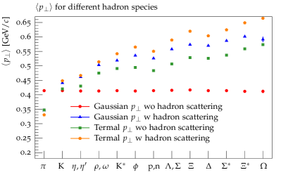


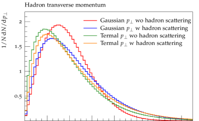
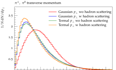


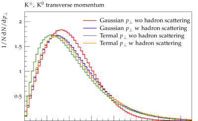
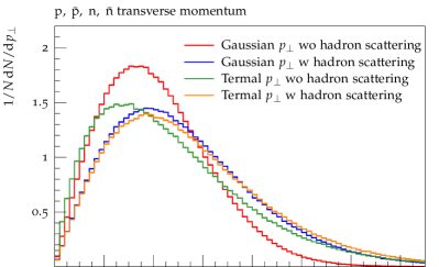


In order to test the hadron scattering a simple toy model is applied: five strings, each with energy , are constructed along the axis with different quark flavours for the endpoint quarks, and the primary produced hadrons are studied. As in section 3.1 the hadrons containing the endpoint quarks are excluded. The following plots are obtained by making use of eqs. (15) and (16); using eq. (17) instead leads to similar results, and thus the same conclusions.
Figure 7 shows the for different hadron species. For the Gaussian hadronic distribution without hadron scattering all hadrons receive the same spectrum. Including hadron scattering, the decreases for pions, the lightest hadrons, by about and increases for heavy hadrons by up more than . The same effect is present for the thermodynamical model, although changes only reach around , as the is higher for heavier hadrons already without hadron rescattering.
Figure 8 shows the normalized spectra for all hadrons and, to exemplify the difference between light and heavy hadrons, the spectrum for pions, kaons, and protons/neutrons. Comparing the inclusive spectrum for the Gaussian , we notice that the distribution gets broader with hadron scattering, i.e. we get more pions with small and more heavy hadrons with higher .
As the thermodynamical model without hadron rescattering comes with a different starting point, compared to the Gaussian model, the effect of the rescattering is not as large, and shifts the spectrum towards larger values. The exception is for pions only, where there is a slight broadening also towards smaller values.
3.4 Results
3.4.1 The Effect of Decays
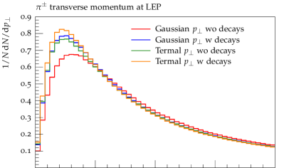
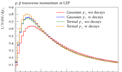


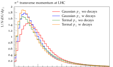
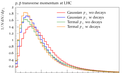


Hadron decays, such as or , influence the spectra of the final state hadrons. As the decays are mostly dictated by kinematics, they constitute a limiting factor on the possibilities of modifying for instance the pion spectrum during the fragmentation process. Even though the primary hadrons follow a Gaussian or exponential distribution, the spectra obtained after decays do not, and become more similar. In addition, in realistic events the effects of perturbative jet production leads to a broadening and the emergence of a powerlike high- tail.
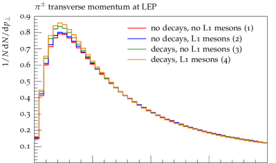
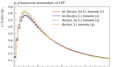
To investigate this smearing of the spectra, we consider realistic jets events and inelastic collisions, where the previously discussed effects of string density and hadron rescattering are not taken into account. The normalized transverse momentum distributions of and are shown in figure 9 for the Gaussian and the thermodynamical model. Comparing the spectra to the previous plots (note the different range of and axis) reveals how much the distributions have moved to higher values, as mentioned above. Four different ratio plots are included for each histogram to investigate different effects: the ratio of distributions after hadronic decays with respect to before, for both models, and the ratio of the thermodynamical with respect to the Gaussian model, with and without decays.
Decays shift the spectra towards smaller values, where the Gaussian model shows a larger change, compared to the thermodynamical model. For LEP the difference between the predictions with and without decays is limited to around at most, while for LHC the changes are rather large, especially for small and large values. Figure 9 also nicely shows that the differences between the Gaussian and thermodynamical model become more than a factor of two smaller when hadronic decays are included, where, as before, the differences are more pronounced for LHC events. Unfortunately, this will limit the impact of the modifications previously discussed in this section.
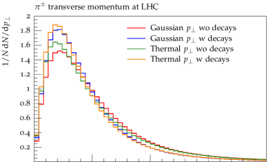
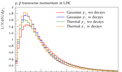


Another question is how much of the hadron rescattering effect on the primary hadrons survives the decays. Note that some of the primary hadrons, such as the meson, are so short-lived that some of their decay products could rescatter which would influence the spectra further. A realistic interleaving of rescattering and decays would require a detailed space–time picture, however, which is for the future.
In figure 10 the pion and proton spectra are shown again for LHC events with hadron rescattering. The same ratio plots as before are included. The ratio of predictions with to without hadron decays shows a similar behaviour as the plots before, where no rescattering was included. The difference between the two models without hadronic decays becomes smaller when hadron rescattering is included. This it not surprising since the effect of the rescattering, that of shuffling some from lighter to heavier hadrons, is smaller in the thermodynamical model where more massive hadrons obtain more already form the beginning. Including decays brings the predictions of the two models even closer together.
3.4.2 Adding more Hadrons
We now briefly investigate the effect of including additional hadrons in the flavour picking process in the thermodynamical model. jets events at are analyzed with the effects of string density and hadron rescattering not being used. As discussed in section 3.2, by default only hadrons with quarks and no radial or orbital excitation are included.
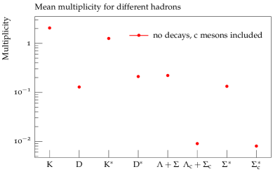
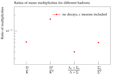
Firstly, consider including hadrons with charm quarks. To obtain a rough estimate of the suppression of production in string breaks, compared to that of quarks, the rates of and mesons and their ratios are analyzed; similar for vector mesons and baryons. The results in figure 11 show that the hadrons are suppressed by more than an order of magnitude compared to hadrons, although a bit less when only vector mesons are considered. In absolute numbers the amount of extra charm production is non-negligible, and probably inconsistent with both LEP and LHC observed rates. Recall that an additional suppression factor for quarks was introduced for the hadron rates in section 3.2; we would therefore expect that a similar, even stronger factor is needed when including quarks in the thermodynamical model. Given this, neither charm nor bottom production is included in the nonperturbative hadronization in the rest of our studies.
Secondly, consider excited mesons by including all of the following meson multiplets, where by default only the first two are present,
-
pseudoscalar multiplet with
-
vector multiplet with
-
pseudovector multiplet with
-
scalar multiplet with
-
pseudovector multiplet with
-
tensor multiplet with
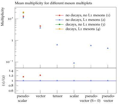
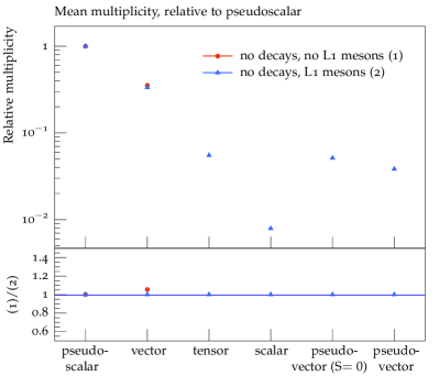
with denoting the sum of the spin and orbital angular momentum in the nonrelativistic approximation. In figure 12 the mean multiplicity of the different multiplets is shown, together with the spectra of pions and protons. Note that including excited mesons leads to an increase of the total meson multiplicity after decays. All multiplets are suppressed by more than an order of magnitude with respect to the pseudoscalar multiplet, with the scalar mesons being suppressed the most due the combination of them being the heaviest of the considered hadrons and their smaller spin-state weight . The normalized spectra exhibit slight shifts towards smaller values, as the now included heavier mesons decay to more lighter hadrons. The excited mesons combined constitute a fraction of roughly of the total meson multiplicity. Given that in addition those mesons and their decay channels are not very well understood, we consider it reasonable to not include those in further studies. In default Pythia the suppression of light vector mesons with respect to pseudoscalar mesons is . The thermodynamical naturally comes with a fairly similar value of .


4 Comparisons with Data
We now proceed to compare the models with data. Note that, in a first step, there is no ambition to obtain a better overall description than the one achieved in several of the standard tunes that come with Pythia. It is rather to explore how the modelling of the new mechanisms impacts selected distributions, notably the ones discussed in section 2.2. That is, whether the mechanisms have the potential to improve the agreement with data in some crucial respects. Only in a second step is there some attempt to combine the various mechanisms, but still without the ambition of a full-fledged tune. In section 4.1 we present a comparison of the different effects we have discussed so far, while section 4.2 gives an overview of the results obtained by combining the effects into a more complete picture. Note that the new mechanisms will be available in the next public Pythia release.
4.1 Impact of the Different Effects
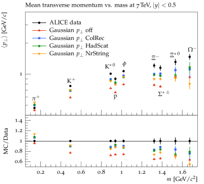
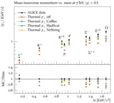
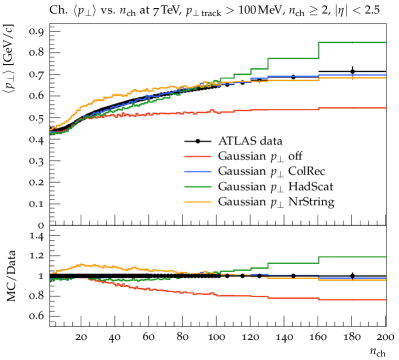
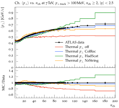
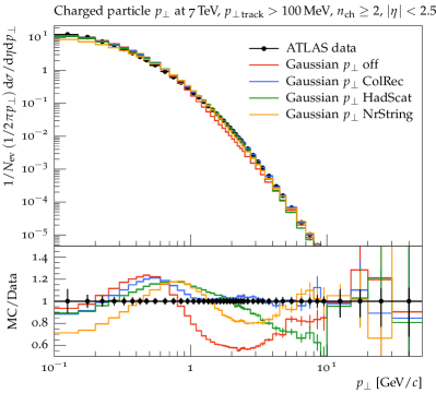
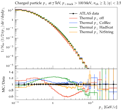
Based on a limited set of LHC observables, this section presents the impact of the new mechanisms outlined in section 3 on the description of data. The observables have been chosen to illustrate the effects of the change of the Gaussian width or temperature, respectively, depending on the close-packing of strings as in eqs. (8) and (14), of hadron rescattering, and of colour reconnection. The latter has been included as it serves a similar purpose and shows a somewhat comparable behaviour. The baseline prediction, which serves as the main comparison for both models, is obtained by switching off all of the aforementioned effects. For a clear picture of the influence of the individual mechanisms, only one of them is switched on at a time. Note that the prediction of the Gaussian model with colour reconnection, labelled “Gaussian ColRec” in the plots, corresponds to default Pythia 8. Recall that the results presented in this subsection are not obtained with parameter settings that optimize the data description but rather illustrate their general effect. The average transverse momentum as a function of the hadron mass and the charged multiplicity are shown in figure 13, together with the charged particle spectrum.
For both models, the description of as a function of mass improves for each of the different mechanisms, compared to the baseline prediction, as heavier hadrons obtain larger values. The thermodynamical model provides a somewhat better description of this observable, compared to the Gaussian model, which comes naturally due to the exponential hadronic transverse-mass suppression.
The baseline prediction for plateaus at small multiplicities, therefore underestimating for values . All of the effects investigated in this study have a somewhat similar effect, in the sense that they are able to push up the prediction, compared to the baseline settings. While including the -dependence significantly improves the description, it is still slightly worse than the prediction with colour reconnection. The hadron rescattering provides a fairly good description of for small values, but clearly overshoots the distribution at high multiplicities.
Similar to the previous observable, the -dependence and colour reconnection improve the description of the inclusive spectrum. The Gaussian model without additional effects switched on produces a bump at and a broad dip at . While colour reconnection removes the dip almost completely, the bump is still clearly visible. The -dependence somewhat reduces both bump and dip, but at the cost of introducing another dip towards very small values. The baseline prediction of the thermodynamical model, compared with the Gaussian one, has the same dip at , while the bump is much less visible. Both colour reconnection and the -dependence reduce the dip quite substantially and provide a very good description of the data. The hadron rescattering, while somewhat improving the description in the low- region, overestimates mid- values by around before undershooting the distribution.
4.2 Results
Using the information of the last subsection we adjust the parameters associated with the new mechanisms to obtain a good data description, with the main focus lying on spectra of pions, kaons, and protons. We begin with LHC data, as this is the motivation for the thermodynamical model, the -dependence, and the hadron rescattering, and continue with a cross-check of some LEP and SLC observables.
4.2.1 LHC
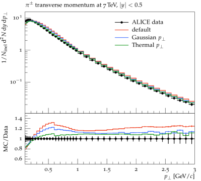
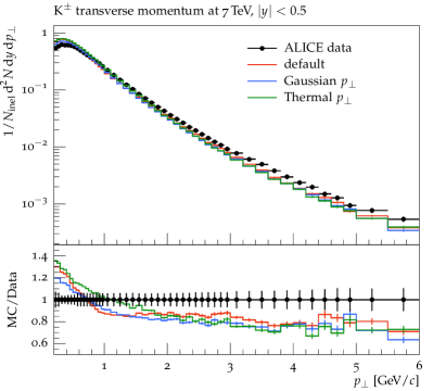
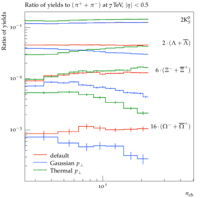
The new parameters are adjusted such that an improvement of the spectra of , and , measured with ALICE Adam:2015qaa , is achieved, while still giving a reasonable description of the charged particle distribution and as a function of the multiplicity, both measured with ATLAS Aad:2010ac . The corresponding settings and values can be found in appendix A. The LHC data set presented here includes the aforementioned spectra and the to ratio shown in figure 14, as a function of the hadron mass and the charged multiplicity, both inclusive and for different hadrons, shown in figure 15, and the ratio of yields with respect to as a function of the charged multiplicity for different hadrons, shown in figure 16. The predictions of default Pythia are compared to the Gaussian and thermodynamical model with the modifications outlined in section 3.
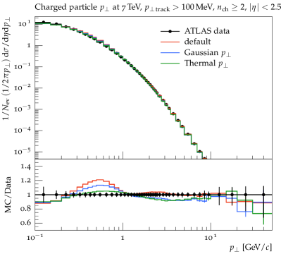
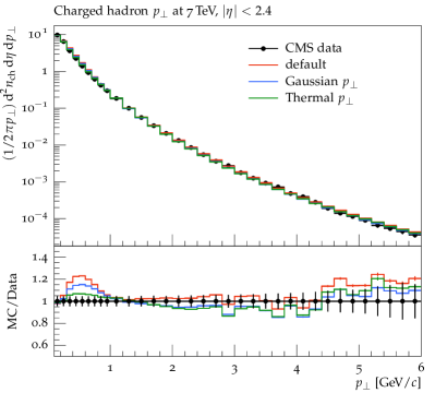
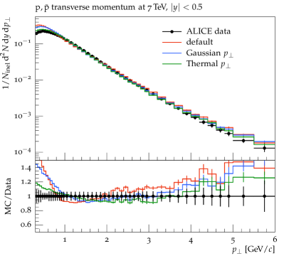




Default Pythia describes the ATLAS charged particle distribution very well for values of , but shows a bump at around . The Gaussian model with modifications gives a similar shape and reduces the bump somewhat, while undershooting the distribution large by a few . The thermodynamical model improves the description quite substantially, especially for low- values, where the aforementioned bump is almost gone. The predictions for the CMS charged hadron spectrum behave mostly similar, with the same bump visible for default Pythia and the Gaussian model.
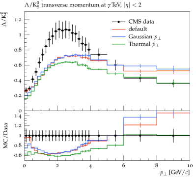
For default Pythia, pions obtain a too hard spectrum. The modifications to the Gaussian model improve the distribution slightly, but there is still no good overall description. With the thermodynamical model the spectrum improves for low- values quite a bit; however, it is still a bit too high in the large- region. The spectrum shows the opposite behaviour: too many soft and too few hard kaons. The Gaussian model with modifications improves the description in the soft region somewhat, compared to default Pythia. Both the Gaussian and thermodynamical model change the shape of the spectrum slightly, but do not provide a better overall description of the . The prediction of both models for the spectrum are better compared to default Pythia, where especially the thermodynamical model improves the low- region quite substantially.
While the prediction of the thermodynamical model for the ratio is somewhat flatter with respect to the data, especially in the low- region, the normalization is off by almost a factor of two due to the combination of producing slightly too many and not enough . The observable could be improved by adjusting the overall normalization factor of baryons with respect to mesons. The value of this parameter has been fixed using the proton spectrum, however.
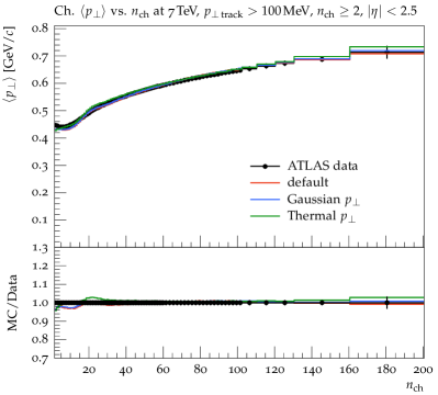
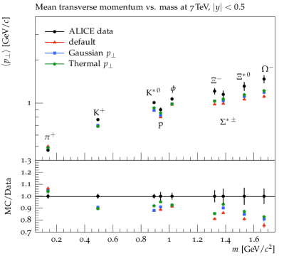
All models give very similar predictions for as a function of , with an extremely good description of the region , but too low for smaller multiplicities. It is quite obvious that the description of this observable could be further improved by choosing a larger value for the width or temperature respectively and simultaneously lowering the -dependence and hadron rescattering. This would however come hand in hand with worse descriptions of other observables. For default Pythia, pions obtain a too large and heavier hadrons a too small one. While the thermodynamical model improves the predictions for , there is still no full agreement with data. The Gaussian model lies in between default Pythia and the thermodynamical model. We observe a similar behaviour for the distribution for individual hadrons. The pion is described fairly well with a slope that is slightly too steep. The main difference of the other hadrons with respect to pions is that they obtain a too small over the whole range. As for pions, the slopes tend to be too steep.
ALICE Adam:2016emw found that the production of strange and multi-strange hadrons is enhanced with increasing multiplicity. While default Pythia is not able to reproduce such a behaviour, figure 16 shows that the thermodynamical model achieves an increase of strangeness with charged multiplicity for , , and , but not for . Except for the latter, we therefore expect the thermodynamical model to give an improved description of the data presented in Adam:2016emw . The Gaussian model with modifications shows the opposite effect, a decrease with growing multiplicity. These findings can be explained as follows: In default Pythia all (primary) hadrons are produced with a probability that is independent of the multiplicity or number of strings. In the thermodynamical model heavier hadrons are produced preferably at large values. Including the -dependence leads to potentially higher temperatures for events with large , where heavy hadrons have a higher probability to be produced, compared to low- events. With the modifications to the Gaussian model, all hadrons obtain more in events with large values of . Due to phase-space constraints heavier hadrons might be rejected more often compared to lower-mass hadrons, leading to the decrease with growing multiplicity. This might also be the reason for the slight drop towards large for in the thermodynamical model, as it eventually dominates over the effect of the -dependence.
4.2.2 LEP and SLC
While the main motivation for introducing the exponential distribution is arising from LHC data, the valid question of whether the same model is able to describe observables as well remains. The effect of the close-packing of strings and hadron rescattering are not included for data as we do not expect them to represent relevant physics here. Furthermore the string dependence relies on rapidity differences and an event axis aligned with the beam, which is not present in collisions.
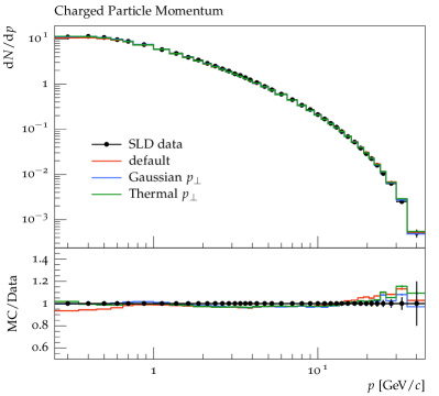
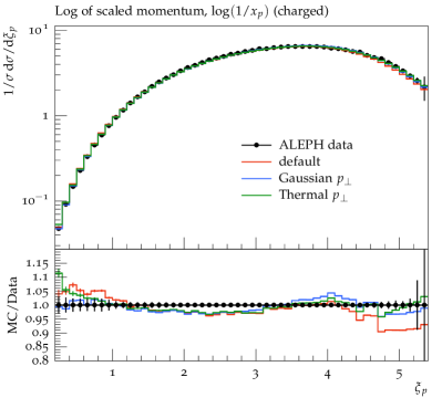
The parameters of the thermodynamical model are adjusted using the charged particle momentum spectrum as well as the scaled momenta of , and , measured with SLD Abe:2003iy , while the ALEPH event shapes Barate:1996fi served as cross checks. For the Gaussian model the width and prefactors for strange and diquarks have been adjusted such that the mean charged multiplicities agrees with the value obtained with the thermodynamical model. The corresponding settings and values can be found in appendix A. The data set presented here includes the aforementioned momenta and mean multiplicities for different hadrons shown in figure 17, as well as the charged multiplicity distribution, scaled momentum and the inclusive and spectra shown in figure 18. The predictions of default Pythia are compared to the Gaussian and thermodynamical model as described above.
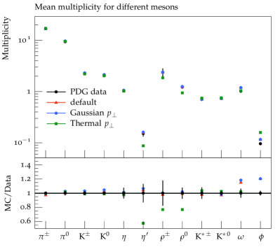
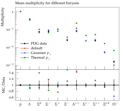
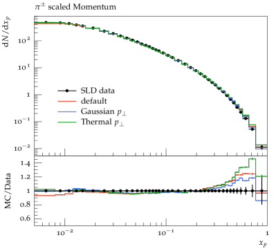
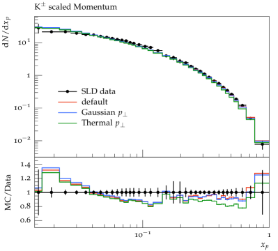
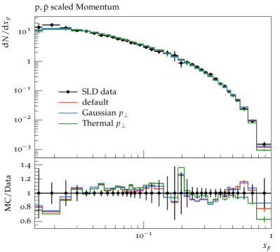
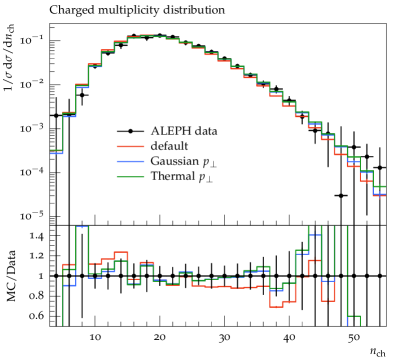
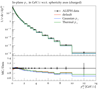
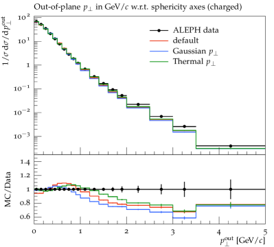
The only difference between default Pythia and the prediction labelled as “Gaussian ” is an adjusted value for the Gaussian width and its prefactors for and diquarks, i.e. there is no change of the flavour selection parameters. Therefore, the values of the mean multiplicities remain, leading to overlapping data and Monte Carlo histogram points in figure 17, which are thus not fully visible. With the thermodynamical model we obtain a fairly good description of most hadrons, with the notable exceptions of producing too many heavy baryons. Note however, that the Gaussian model comes with around 20 parameter for selecting the flavour of new hadrons, whereas the thermodynamical model makes use of only three parameters: the temperature, the overall normalization factor of baryons with respect to mesons, and the additional suppression factor for hadrons with strange quarks, see section 3.2. Hence, the result is fairly acceptable.
The predictions of the two models for the charged particle momentum agree very well with data in the soft region; there is only some small deviation for medium and large momenta, where especially the thermodynamical model predicts somewhat too many particles in the hard region. The same effect is even clearer visible in the scaled momentum spectrum of pions. For kaons and protons we observe the opposite effect: the new model predicts too few hadrons with large momenta.
Similar to the charged particle momentum, the predictions of both models for the logarithm of the scaled momentum agrees well with data, with some small deviation for medium and large values. However, the sudden drop in the ratio of the Monte Carlo prediction to data at around remains almost unchanged. The description of the charged multiplicity distribution improves slightly, compared to default Pythia, towards having less events with small multiplicities and more events with larger ones. This is due to having an increased mean charged multiplicity. While both models describe the low- region of the inclusive and spectra very well, they underestimate the amount of events with larger values. The thermodynamical model provides a better description of especially the spectrum, compared to the Gaussian model.
To summarize we note that the thermodynamical model is able to provide predictions for event shapes and momentum spectra in events that are of a similar quality as those by the Gaussian model. Nevertheless, the hadron decomposition is not described well, a price to pay for reducing the amount of flavour selection parameters.
5 Summary and Outlook
The understanding of soft hadronic physics is changing under the onslaught of LHC pp data. Of course, there has never been an approach that could describe all aspects of pp physics perfectly, but before LHC it was often assumed that all the basic concepts were in place, and that what remained was successive refinements. Now we see that there is still much left to learn. There have already been several surprises, and further data analyses may well produce more.
In view of this we have revisited some of the basic soft-physics assumptions of the Pythia event generator, which has been quite successful in predicting and describing many aspects of the data, but now starts to show cracks. New approaches have here been studied for some areas, to understand how much room for improvements there would be, without any claim that either of them would necessarily be the one and only right way to go.
A central pillar of Pythia has been the Lund string fragmentation model, where a tunneling mechanism for string breakups leads to a universal Gaussian spectrum. In this work a thermodynamical model is implemented as an alternative, where instead follows an exponential distribution. For an already selected , the hadron flavour is picked based on an exponential weight, with additional factors due to spin-counting rules and so on. This approach suppresses the production of heavier hadrons, and gives them a larger . Such a pattern is observed in data, and exists in the Gaussian approach mainly owing to particle decays, but there undershoots data.
Making the Gaussian width, or temperature in case of the thermodynamical model, dependent on the close-packing of strings allows for modelling the influence of strings on each other in a simple way. An effective number of density of strings is introduced for low ’s, while high- fragmentation tends to occur outside the close-packed string region and is left unaffected. Such a mechanism could e.g. be used to explain a changing flavour composition at high multiplicities.
Finally we implemented a simple model for hadronic rescattering, applied to the primary hadrons, before decays. The probability of two hadrons to rescatter is based on how close they are in phase space. By favouring a shift towards equal transverse velocities, it should also give higher for heavy hadrons and lower for pions.
Not surprisingly we found the hadronic decays to limit the hoped-for effects. Specifically, most pions come from decays of heavier hadrons, and so the mechanisms intended to give less to pions and more to kaons and protons are largely nullified. The mechanisms are also not simply additive; starting out from the thermodynamical model with its already-existing mass differentiation, the further effects of varying temperatures or hadronic rescattering are smaller than corresponding effects in the Gaussian approach.
Nevertheless the thermodynamical model is able to provide reasonable descriptions of observables such as the spectrum of charged hadrons, the average transverse momentum as a function of the hadron mass, or the recently measured enhanced production of strange and multi-strange hadrons with increasing multiplicity. These observables have so far been described rather poorly by Pythia. And, given the small number of flavour parameters in the thermodynamical model, it is able to describe a reasonable number of data rather well, even if it can not compete with the many-more-parameter tunes of default Pythia.
It should be noted that we have not compared with all relevant available data, by far. Notably, the ridge effect was not described by the existing Pythia model, and our current changes do not introduce any mechanism to induce it. The ridge was first observed in AA collisions Adams:2005ph ; Abelev:2009af ; Alver:2009id ; Chatrchyan:2011eka , where nuclear geometry and hydrodynamical expansion offer natural starting points Ollitrault:1992bk ; Voloshin:1994mz , although the range of detailed models is too vast to cover here Akiba:2015jwa . In the field of pp physics Li:2012hc , the EPOS model addresses the issue by having an inner core that can push strings in the outer corona Werner:2010ss , whereas a recent extension of DIPSY Bierlich:2016vgw provides a corresponding shove from the excess energy of central overlapping strings that form ropes. In a similar spirit, our higher string tension could introduce a push also without rope formation. A detailed modelling is not trivial, however, and we have not pursued it for now.
To advance to the next level of sophistication within the line of research advocated here, it would be necessary to do a microscopic tracing of the full space–time evolution of the event, both for partons and for hadrons, and including both production and decay vertices. This is nontrivial beyond the simple one-string picture, even in the cleaner events, and the further complications of MPIs and CR in hadronic events will make it even worse. What it would allow is a more detailed understanding of the close-packing both of strings and of hadrons. Combined with a more detailed modelling of hadronic rescattering, a more realistic picture may emerge.
Some of the limitations encountered here are likely still to remain, so further mechanisms may be at play, in addition to the ones studied here. This would not be the first time where a cocktail of smaller effects combine to give a significant signal. What is less likely is actually the opposite, that one single mechanism does it all. Specifically, whatever else may be going on, the close-packing of strings and hadrons appears unavoidable in high-multiplicity pp events, and collective-flow effects are here to stay. In sum, we have an interesting and challenging time ahead of us, where some of the most unexpected new LHC observations may well come in the low- region rather than the in high- one.
Acknowledgements
Helpful discussions with Peter Skands are gratefully acknowledged. Work supported by the MCnetITN FP7 Marie Curie Initial Training Network, contract PITN-GA-2012-315877. This project has also received funding in part by the Swedish Research Council, contract number 621-2013-4287, and in part from the European Research Council (ERC) under the European Union’s Horizon 2020 research and innovation programme (grant agreement No 668679).
Appendix A Settings
Table 1 gives a list of the settings that have been changed with respect to default Pythia to obtain the results presented in section 4.2.
| LHC | LEP and SLC | ||||
|---|---|---|---|---|---|
| Default | Gaussian | Thermal | Gaussian | Thermal | |
| Switch to thermal model? | |||||
| StringPT:thermalModel | off | off | on | off | on |
| Gaussian width | |||||
| StringPT:sigma | 0.335 | 0.33 | - | 0.295 | - |
| prefactor for quarks | |||||
| StringPT:widthPreStrange | 1.0 | 1.2 | - | 1.2 | - |
| prefactor for diquarks | |||||
| StringPT:widthPreDiquark | 1.0 | 1.2 | - | 1.2 | - |
| Fraction with enhanced | |||||
| StringPT:enhancedFraction | 0.01 | 0.0 | - | 0.0 | - |
| Temperature | |||||
| StringPT:temperature | - | - | 0.21 | - | 0.205 |
| Baryon normalization factor | |||||
| StringFlav:BtoMratio | - | - | 0.357 | - | 0.625 |
| Suppression factor for hadrons | |||||
| StringFlav:StrangeSuppression | - | - | 0.5 | - | 0.45 |
| parameter in eq. (8) or (14) | |||||
| StringPT:expNSP | 0.0 | 0.01 | 0.13 | 0.0 | 0.0 |
| Range of MPI-based CR scheme | |||||
| ColourReconnection:range | 1.8 | 1.8 | 1.1 | - | - |
| Hadron rescattering (HR) on? | |||||
| HadronLevel:HadronScatter | off | on | on | off | off |
| HR with eq. (15) and (16) | |||||
| HadronScatter:mode | - | 0 | 0 | - | - |
| parameter in eq. (16) | |||||
| HadronScatter:maxProbDS | - | 0.25 | 0.5 | - | - |
| MPI regularization parameter | |||||
| MultipartonInteractions:pT0Ref | 2.28 | 2.34 | 2.5 | - | - |
References
- (1) G. P. Salam, QCD Theory Overview — Towards Precision at LHC, 2016.
- (2) B. Andersson, G. Gustafson, G. Ingelman and T. Sjöstrand, Parton Fragmentation and String Dynamics, Phys. Rept. 97 (1983) 31–145.
- (3) R. D. Field and S. Wolfram, A QCD Model for Annihilation, Nucl. Phys. B213 (1983) 65.
- (4) T. D. Gottschalk, An improved description of hadronization in the QCD cluster model for annihilation, Nucl. Phys. B239 (1984) 349.
- (5) B. R. Webber, A QCD Model for Jet Fragmentation Including Soft Gluon Interference, Nucl. Phys. B238 (1984) 492.
- (6) A. Ortiz Velasquez, P. Christiansen, E. Cuautle Flores, I. Maldonado Cervantes and G. Paic, Color Reconnection and Flowlike Patterns in Collisions, Phys. Rev. Lett. 111 (2013) 042001, [1303.6326].
- (7) CMS collaboration, V. Khachatryan et al., Observation of Long-Range Near-Side Angular Correlations in Proton-Proton Collisions at the LHC, JHEP 09 (2010) 091, [1009.4122].
- (8) ATLAS collaboration, G. Aad et al., Observation of Long-Range Elliptic Azimuthal Anisotropies in 13 and 2.76 TeV Collisions with the ATLAS Detector, Phys. Rev. Lett. 116 (2016) 172301, [1509.4776].
- (9) CMS collaboration, V. Khachatryan et al., Evidence for collectivity in pp collisions at the LHC, 1606.6198.
- (10) ALICE collaboration, J. Adam et al., Multiplicity-dependent enhancement of strange and multi-strange hadron production in proton-proton collisions at TeV, 1606.7424.
- (11) E. Cuautle and G. Paic, The energy density representation of the strangeness enhancement from p+p to Pb+Pb, 1608.02101.
- (12) P. Braun-Munzinger and J. Stachel, The quest for the quark-gluon plasma, Nature 448 (2007) 302–309.
- (13) T. Pierog, I. Karpenko, J. M. Katzy, E. Yatsenko and K. Werner, EPOS LHC: Test of collective hadronization with data measured at the CERN Large Hadron Collider, Phys. Rev. C92 (2015) 034906, [1306.0121].
- (14) T. S. Biro, H. B. Nielsen and J. Knoll, Color Rope Model for Extreme Relativistic Heavy Ion Collisions, Nucl. Phys. B245 (1984) 449–468.
- (15) A. Bialas and W. Czyz, Chromoelectric Flux Tubes and the Transverse Momentum Distribution in High-energy Nucleus-nucleus Collisions, Phys. Rev. D31 (1985) 198.
- (16) B. Andersson and P. A. Henning, On the dynamics of a color rope: The Fragmentation of interacting strings and the longitudinal distributions, Nucl. Phys. B355 (1991) 82–105.
- (17) C. Bierlich, G. Gustafson, L. Lönnblad and A. Tarasov, Effects of Overlapping Strings in pp Collisions, JHEP 03 (2015) 148, [1412.6259].
- (18) P. Capiluppi, G. Giacomelli, A. M. Rossi, G. Vannini and A. Bussiere, Transverse momentum dependence in proton proton inclusive reactions at very high energies, Nucl. Phys. B70 (1974) 1–38.
- (19) R. Hagedorn, Statistical thermodynamics of strong interactions at high-energies, Nuovo Cim. Suppl. 3 (1965) 147–186.
- (20) R. Hagedorn, Remarks on the thermodynamical model of strong interactions, Nucl. Phys. B24 (1970) 93–139.
- (21) R. Hagedorn, Multiplicities, Distributions and the Expected Hadron Quark - Gluon Phase Transition, Riv. Nuovo Cim. 6N10 (1983) 1–50.
- (22) S. Barshay and Y. A. Chao, Longitudinal mass, inclusive transverse-momentum distributions, proton proton elastic diffraction slopes and the total cross-section, Phys. Lett. B38 (1972) 225–228.
- (23) C. Tsallis, Possible Generalization of Boltzmann-Gibbs Statistics, J. Statist. Phys. 52 (1988) 479–487.
- (24) J. Cleymans, On the Use of the Tsallis Distribution at LHC Energies, in 16th International Conference on Strangeness in Quark Matter (SQM 2016) Berkeley, California, United States, June 27-July 1, 2016, 2016. 1609.02289.
- (25) A. A. Bylinkin and A. A. Rostovtsev, Parametrization of the shape of hadron-production spectra in high-energy particle interactions, Phys. Atom. Nucl. 75 (2012) 999–1005.
- (26) T. Sjöstrand and M. van Zijl, A Multiple Interaction Model for the Event Structure in Hadron Collisions, Phys. Rev. D36 (1987) 2019.
- (27) T. Sjöstrand, S. Mrenna and P. Z. Skands, PYTHIA 6.4 Physics and Manual, JHEP 05 (2006) 026, [hep-ph/0603175].
- (28) T. Sjöstrand, S. Ask, J. R. Christiansen, R. Corke, N. Desai, P. Ilten et al., An Introduction to PYTHIA 8.2, Comput. Phys. Commun. 191 (2015) 159–177, [1410.3012].
- (29) X. Artru and G. Mennessier, String model and multiproduction, Nucl. Phys. B70 (1974) 93–115.
- (30) B. Andersson, G. Gustafson and B. Söderberg, A Probability Measure on Parton and String States, Nucl. Phys. B264 (1986) 29.
- (31) G. ’t Hooft, A planar diagram theory for strong interactions, Nucl. Phys. B72 (1974) 461.
- (32) B. Andersson, G. Gustafson and T. Sjöstrand, How to Find the Gluon Jets in e+ e- Annihilation, Phys. Lett. B94 (1980) 211–215.
- (33) JADE collaboration, W. Bartel et al., Experimental Study of Jets in electron - Positron Annihilation, Phys. Lett. B101 (1981) 129–134.
- (34) T. Sjöstrand, Jet fragmentation of nearby partons, Nucl. Phys. B248 (1984) 469.
- (35) T. Sjöstrand and P. Z. Skands, Baryon number violation and string topologies, Nucl. Phys. B659 (2003) 243, [hep-ph/0212264].
- (36) B. Andersson, G. Gustafson and T. Sjöstrand, On Soft Gluon Emission and the Transverse Momentum Properties of Final State Particles, Z. Phys. C12 (1982) 49.
- (37) F. E. Close, An Introduction to Quarks and Partons. 1979.
- (38) B. Andersson, G. Gustafson and T. Sjöstrand, A Model for Baryon Production in Quark and Gluon Jets, Nucl. Phys. B197 (1982) 45–54.
- (39) B. Andersson, G. Gustafson and T. Sjöstrand, Baryon Production in Jet Fragmentation and Upsilon-Decay, Phys. Scripta 32 (1985) 574.
- (40) S. Plätzer and S. Gieseke, Dipole Showers and Automated NLO Matching in Herwig++, Eur. Phys. J. C72 (2012) 2187, [1109.6256].
- (41) P. Richardson and D. Winn, Investigation of Monte Carlo Uncertainties on Higgs Boson searches using Jet Substructure, Eur. Phys. J. C72 (2012) 2178, [1207.0380].
- (42) S. Chun and C. Buchanan, A Simple plausible path from QCD to successful prediction of e+ e- hadronization data, Phys. Rept. 292 (1998) 239–317.
- (43) S. Abachi, C. Buchanan, A. Chien, S. Chun and B. Hartfiel, UCLA space-time area law model: A Persuasive foundation for hadronization, Eur. Phys. J. C49 (2007) 569–580, [hep-ph/0612103].
- (44) A. Buckley et al., Rivet user manual, 1003.0694.
- (45) STAR collaboration, B. I. Abelev et al., Systematic Measurements of Identified Particle Spectra in Au and Au+Au Collisions from STAR, Phys. Rev. C79 (2009) 034909, [0808.2041].
- (46) ALICE collaboration, B. B. Abelev et al., Production of and in proton-proton collisions at 7 TeV, Eur. Phys. J. C75 (2015) 1, [1406.3206].
- (47) ATLAS collaboration, G. Aad et al., Charged-particle multiplicities in pp interactions measured with the ATLAS detector at the LHC, New J. Phys. 13 (2011) 053033, [1012.5104].
- (48) ALICE collaboration, L. Bianchi, Strangeness production as a function of charged particle multiplicity in proton-proton collisions, 1604.6736.
- (49) CMS collaboration, S. Chatrchyan et al., Charged particle transverse momentum spectra in collisions at and 7 TeV, JHEP 08 (2011) 086, [1104.3547].
- (50) ALICE collaboration, J. Adam et al., Pseudorapidity and transverse-momentum distributions of charged particles in proton-proton collisions at 13 TeV, Phys. Lett. B753 (2016) 319–329, [1509.8734].
- (51) ALICE collaboration, J. Adam et al., Measurement of pion, kaon and proton production in proton-proton collisions at TeV, Eur. Phys. J. C75 (2015) 226, [1504.0024].
- (52) CMS collaboration, V. Khachatryan et al., Strange Particle Production in Collisions at and 7 TeV, JHEP 05 (2011) 064, [1102.4282].
- (53) UA1 collaboration, C. Albajar et al., A Study of the General Characteristics of Collisions at = 0.2-TeV to 0.9-TeV, Nucl. Phys. B335 (1990) 261–287.
- (54) T. Sjöstrand and V. A. Khoze, On Color rearrangement in hadronic events, Z. Phys. C62 (1994) 281–310, [hep-ph/9310242].
- (55) J. R. Christiansen and P. Z. Skands, String Formation Beyond Leading Colour, JHEP 08 (2015) 003, [1505.01681].
- (56) A. Chodos, R. L. Jaffe, K. Johnson, C. B. Thorn and V. F. Weisskopf, A New Extended Model of Hadrons, Phys. Rev. D9 (1974) 3471–3495.
- (57) H. Sorge, H. Stoecker and W. Greiner, Poincare Invariant Hamiltonian Dynamics: Modeling Multi - Hadronic Interactions in a Phase Space Approach, Annals Phys. 192 (1989) 266–306.
- (58) H. Sorge, M. Berenguer, H. Stoecker and W. Greiner, Color rope formation and strange baryon production in ultrarelativistic heavy ion collisions, Phys. Lett. B289 (1992) 6–11.
- (59) S. A. Bass et al., Microscopic models for ultrarelativistic heavy ion collisions, Prog. Part. Nucl. Phys. 41 (1998) 255–369, [nucl-th/9803035].
- (60) M. Bleicher et al., Relativistic hadron hadron collisions in the ultrarelativistic quantum molecular dynamics model, J. Phys. G25 (1999) 1859–1896, [hep-ph/9909407].
- (61) S. Soff, D. Zschiesche, M. Bleicher, C. Hartnack, M. Belkacem, L. Bravina et al., Enhanced strange particle yields - signal of a phase of massless particles?, J. Phys. G27 (2001) 449–458, [nucl-th/0010103].
- (62) S. Soff, J. Randrup, H. Stoecker and N. Xu, Effects of strong color fields on baryon dynamics, Phys. Lett. B551 (2003) 115–120, [nucl-th/0209093].
- (63) B. Zhang, C. M. Ko, B.-A. Li and Z.-w. Lin, A multiphase transport model for nuclear collisions at RHIC, Phys. Rev. C61 (2000) 067901, [nucl-th/9907017].
- (64) Z.-W. Lin, C. M. Ko, B.-A. Li, B. Zhang and S. Pal, A Multi-phase transport model for relativistic heavy ion collisions, Phys. Rev. C72 (2005) 064901, [nucl-th/0411110].
- (65) Z.-w. Lin, S. Pal, C. M. Ko, B.-A. Li and B. Zhang, Charged particle rapidity distributions at relativistic energies, Phys. Rev. C64 (2001) 011902, [nucl-th/0011059].
- (66) N. S. Amelin, M. A. Braun and C. Pajares, Multiple production in the Monte Carlo string fusion model, Phys. Lett. B306 (1993) 312–318.
- (67) N. S. Amelin, N. Armesto, C. Pajares and D. Sousa, Monte Carlo model for nuclear collisions from SPS to LHC energies, Eur. Phys. J. C22 (2001) 149–163, [hep-ph/0103060].
- (68) M. A. Braun and C. Pajares, Particle production in nuclear collisions and string interactions, Phys. Lett. B287 (1992) 154–158.
- (69) M. A. Braun and C. Pajares, Implications of percolation of color strings on multiplicities, correlations and the transverse momentum, Eur. Phys. J. C16 (2000) 349–359, [hep-ph/9907332].
- (70) M. A. Braun and C. Pajares, Transverse momentum distributions and their forward backward correlations in the percolating color string approach, Phys. Rev. Lett. 85 (2000) 4864–4867, [hep-ph/0007201].
- (71) C. Pajares, String and parton percolation, Eur. Phys. J. C43 (2005) 9–14, [hep-ph/0501125].
- (72) Particle Data Group collaboration, C. Amsler et al., Review of Particle Physics, Phys. Lett. B667 (2008) 1–1340.
- (73) British-Scandinavian collaboration, B. Alper et al., Production Spectra of pi+-, K+-, rho+- at Large Angles in Proton Proton Collisions in the CERN Intersecting Storage Rings, Nucl. Phys. B100 (1975) 237–290.
- (74) British-Scandinavian-MIT collaboration, K. Guettler et al., Inclusive Production of Low-Momentum Charged Pions at at the CERN Intersecting Storage Rings, Phys. Lett. B64 (1976) 111–116.
- (75) G. Giacomelli and M. Jacob, Physics at the CERN ISR, Phys. Rept. 55 (1979) 1–132.
- (76) I. S. Gradshteyn and I. M. Ryzhik, Table of Integrals, Series, and Products, Fourth Edition. Academic Press, London, 1980.
- (77) M. Abramowitz and I. Stegun, Handbook of Mathematical Functions with Formulas, Graphs, and Mathematical Tables. Dover Publications, New York, 1965.
- (78) J. Dias de Deus and C. Pajares, Percolation of color sources and critical temperature, Phys. Lett. B642 (2006) 455–458, [hep-ph/0607101].
- (79) M. Gyulassy and L. McLerran, New forms of QCD matter discovered at RHIC, Nucl. Phys. A750 (2005) 30–63, [nucl-th/0405013].
- (80) U. Heinz and R. Snellings, Collective flow and viscosity in relativistic heavy-ion collisions, Ann. Rev. Nucl. Part. Sci. 63 (2013) 123–151, [1301.2826].
- (81) G. Roland, K. Safarik and P. Steinberg, Heavy-ion collisions at the LHC, Prog. Part. Nucl. Phys. 77 (2014) 70–127.
- (82) R. D. Field and R. P. Feynman, A parametrization of the properties of quark jets, Nucl. Phys. B136 (1978) 1.
- (83) CMS collaboration, V. Khachatryan et al., Transverse-momentum and pseudorapidity distributions of charged hadrons in collisions at TeV, Phys. Rev. Lett. 105 (2010) 022002, [1005.3299].
- (84) SLD collaboration, K. Abe et al., Production of pi+, pi-, K+, K-, p and anti-p in light (uds), c and b jets from Z0 decays, Phys. Rev. D69 (2004) 072003, [hep-ex/0310017].
- (85) ALEPH collaboration, R. Barate et al., Studies of quantum chromodynamics with the ALEPH detector, Phys. Rept. 294 (1998) 1–165.
- (86) STAR collaboration, J. Adams et al., Distributions of charged hadrons associated with high transverse momentum particles in pp and Au + Au collisions at s(NN)**(1/2) = 200-GeV, Phys. Rev. Lett. 95 (2005) 152301, [nucl-ex/0501016].
- (87) STAR collaboration, B. I. Abelev et al., Long range rapidity correlations and jet production in high energy nuclear collisions, Phys. Rev. C80 (2009) 064912, [0909.0191].
- (88) PHOBOS collaboration, B. Alver et al., High transverse momentum triggered correlations over a large pseudorapidity acceptance in Au+Au collisions at s(NN)**1/2 = 200 GeV, Phys. Rev. Lett. 104 (2010) 062301, [0903.2811].
- (89) CMS collaboration, S. Chatrchyan et al., Long-range and short-range dihadron angular correlations in central PbPb collisions at a nucleon-nucleon center of mass energy of 2.76 TeV, JHEP 07 (2011) 076, [1105.2438].
- (90) J.-Y. Ollitrault, Anisotropy as a signature of transverse collective flow, Phys. Rev. D46 (1992) 229–245.
- (91) S. Voloshin and Y. Zhang, Flow study in relativistic nuclear collisions by Fourier expansion of Azimuthal particle distributions, Z. Phys. C70 (1996) 665–672, [hep-ph/9407282].
- (92) Y. Akiba et al., The Hot QCD White Paper: Exploring the Phases of QCD at RHIC and the LHC, 1502.02730.
- (93) W. Li, Observation of a ’Ridge’ correlation structure in high multiplicity proton-proton collisions: A brief review, Mod. Phys. Lett. A27 (2012) 1230018, [1206.0148].
- (94) K. Werner, I. Karpenko and T. Pierog, The ’Ridge’ in Proton-Proton Scattering at 7 TeV, Phys. Rev. Lett. 106 (2011) 122004, [1011.0375].
- (95) C. Bierlich, G. Gustafson and L. Lönnblad, A shoving model for collectivity in hadronic collisions, 1612.05132.