Robust Gait Recognition by Integrating Inertial and RGBD Sensors
Abstract
Gait has been considered as a promising and unique biometric for person identification. Traditionally, gait data are collected using either color sensors, such as a CCD camera, depth sensors, such as a Microsoft Kinect, or inertial sensors, such as an accelerometer. However, a single type of sensors may only capture part of the dynamic gait features and make the gait recognition sensitive to complex covariate conditions, leading to fragile gait-based person identification systems. In this paper, we propose to combine all three types of sensors for gait data collection and gait recognition, which can be used for important identification applications, such as identity recognition to access a restricted building or area. We propose two new algorithms, namely EigenGait and TrajGait, to extract gait features from the inertial data and the RGBD (color and depth) data, respectively. Specifically, EigenGait extracts general gait dynamics from the accelerometer readings in the eigenspace and TrajGait extracts more detailed sub-dynamics by analyzing 3D dense trajectories. Finally, both extracted features are fed into a supervised classifier for gait recognition and person identification. Experiments on 50 subjects, with comparisons to several other state-of-the-art gait-recognition approaches, show that the proposed approach can achieve higher recognition accuracy and robustness.
Index Terms:
Gait recognition, multi-sensor integration, person identification, dense trajectory, accelerometer.I Introduction
Using gait, or the manner of walking, for person identification has been drawing more and more attention in recent years [1, 2, 3], due to its capability to recognize a person at a longer distance than the traditional biometrics based on face, fingerprint and iris recognition. However, in practice gait biometrics usually suffer from two issues. First, the data collected by a single type of sensors, e.g., a CCD camera, may only capture part of the gait features and this may limit the gait recognition accuracy. Second, gait biometrics are usually sensitive to hard-covariate conditions, e.g., walking with hands in pocket or with loadings. In this paper, we propose to combine gait data collected by different types of sensors to promote the gait recognition accuracy and the robustness.
In the previous research, three types of sensors have been used for gait data collection and gait recognition – color sensors, depth sensors and inertial sensors. Using color sensors, e.g., CCD cameras, a walking person can be captured into a video, in which each frame is a 2D RGB (color) image of the person and the surrounding environment. Gait recognition on such a video is usually achieved by segmenting, tracking, and analyzing the silhouette of the walking person on each frame [4, 5, 6, 7, 8, 9, 10, 11]. The silhouette segmentation and tracking can be difficult when the color of the person is similar to the color of the surrounding environment in the video. In addition, color sensors generally capture the dynamic gait features in a 2D space.
Using depth sensors, such as the line-structure light devices, it is usually easier to segment a walking person from the surrounding environment, when there is no other moving objects around. In addition, from the depth data, 3D dynamic gait features can be derived for gait recognition [12, 13, 14]. However, in practice depth data may contain noise and errors, especially at the spots with strong reflectiveness, e.g., on a reflective clothing, where the depth value is totally invalid. Such errors may lead to incorrect gait features and gait recognition results.
Different from color and depth sensors, which are installed to capture the walking person at a distance to collect gait data, inertial sensors such as accelerometers and gyroscopes collect gait data by attaching to and moving with the person [15, 16, 17, 18, 19, 20, 21]. The inertial-sensor based gait recognition mainly benefits from the extensive use of smart phones – people always carry their smart phones and almost all the smart phones have integrated inertial sensors of accelerometers and gyroscopes. Considering the usability, the smart phone must be allowed to be placed in any pockets with different orientations when we use its inertial sensors for gait recognition. Such different placements and orientations of the sensors may vary the inertial data and affect the gait recognition accuracy [18].
In general, each type of the above-mentioned sensors can capture part of the gait features with different kinds of errors and incompleteness. For example, depth and inertial sensors capture 3D gait features and color sensors capture 2D gait features. Meanwhile, the inertial data, such as the accelerometer readings, portrait the motion pattern of the whole body and provide a general description to the gait dynamics, while the color and depth data can be used to infer the motion of many body parts and provide more detailed sub-dynamics of the gait. It is natural to assume that the gait features derived from different sensors can complement each other. This motivates the proposed approach to integrate the color, depth and inertial sensors for more accurate gait recognition.
Sensitivity to complex covariate conditions is another main issue in gait biometrics [6]. For example, gait data from a sensor may look different when the same person walks with hands in pocket or with loadings. Such a difference increases the variance of a person’s gait features and reduces the gait recognition accuracy. In this paper, through carefully designed experiments, we show that the proposed approach of integrating different sensors can also improve the robustness of gait recognition under complex covariate conditions.
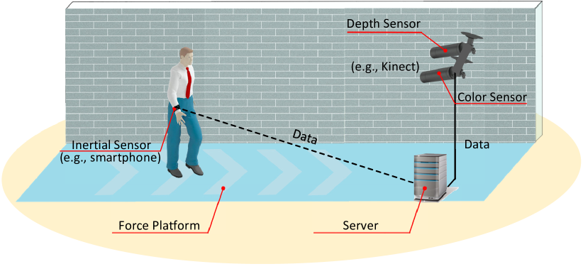
As a practical application scenario, the proposed approach of integrating different sensors for gait recognition can be used for person identification to access a restricted area or building. As illustrated in Fig. 1, at the entrance of a restricted area, a user simply walks on a force platform to get his identity verified. During his walk, a pre-installed client application in his smart phone sends real-time inertial-sensor readings to the server by wireless communication. At the same time, color and depth sensors, mounted over the ceiling and facing the platform, collect the RGBD (color and depth) data and send them to the server. In the server, the proposed approach can integrate all the data and perform gait recognition to identify whether he is an authorized user or not. Other than a higher gait recognition accuracy, such an identification system also has good security – even if the smart phone is hacked to send forged inertial data to the server, it is difficult to forge the RGBD data since color and depth sensors are not controlled by the user.
Following the scheme of identification illustrated in Fig. 1, in this paper we use accelerometer in the smart phone to collect inertial data and Microsoft Kinect to collect the RGBD (color and depth) data. We develop a new EigenGait algorithm to capture the general gait dynamics by analyzing the inertial data in the eigenspace and a new TrajGait algorithm to capture more detailed gait sub-dynamics based on the 3D trajectories extracted from the RGBD video. The extracted features on general dynamics and sub-dynamics of gait are then integrated and fed into a supervised classifier for gait recognition and person identification. In the experiments, we collect three sets of inertial and RGBD data from 50 subjects and evaluate the proposed approach under various covariate conditions. Comparison results with other approaches confirm that the gait recognition accuracy and robustness can be improved by integrating different types of sensors. The main contributions of this paper lie in four-fold.
-
First, a multi-sensor integration method is proposed for gait recognition, in which inertial sensor, color sensor and depth sensor are integrated to capture gait dynamics. The multi-sensor data fusion leads to more robust gait-recognition performance.
-
Second, an EigenGait algorithm is developed to describe the general gait dynamics by analyzing the time-series acceleration data in the eigenspace. The extracted features are more effective than that produced by Fast Fourier Transforms (FFT) or Wavelet Transforms.
-
Third, a TrajGait algorithm is proposed to describe the detailed sub-dynamics of gait by analyzing the RGBD videos. In TrajGait, 3D dense trajectories are derived from the RGBD videos and used for representing the gait features. We found that such gait features are more discriminative than the depth- or skeleton- based features in gait recognition.
-
Finally, three new datasets, with both RGBD and accelerometer data, are collected on 50 subjects. They can be used to quantitatively evaluate and compare the performance of different gait recognition methods.
The remainder of this paper is organized as follows. Section II reviews the related work. Section III introduces the proposed approach, including sensor setting, data collection, gait feature extraction, and integrated gait recognition. Section IV reports the experiments and results. Section V concludes our work and briefly discuss the possible future work.
II Related Work
The ideas and experiments of gait recognition can be traced back to Cutting and Kozlowski’s work [22], in which the manner of walking, i.e., the gait, was found to be possible to identify a person. Since then, gait-based person identification has attracted extensive attention in both academia and industry [23], and a number of gait recognition methods have been proposed. In these methods, three types of sensors are mainly used for gait data collection, namely the color sensor, the depth sensor, and the inertial sensor. Hence, the gait recognition methods can be classified into the color-based, the depth-based, and the inertia-based. In this section, we briefly overview them, as well as a brief overview to other action-based biometrics.
Color-based methods. The color-based methods had a rapid development in the early days [4, 24, 25, 5, 26, 6, 27, 28, 29, 30, 31]. These methods can be classified into the model-free methods and the model-based methods. In the model-free methods, gait features are often extracted by analyzing the shapes, or contours, of the silhouettes in successive frames. In addition, features on the velocity, texture and color are also examined. One important work among them is the GEI (gait energy image) method [5], which represents gait dynamics by an aligned and normalized silhouettes over a gait cycle. The GEI provides a compact representation of the spatial occupancy of a person over a gait cycle. However, partitioning gait cycles from a color video is rarely easy. In [25, 32], silhouettes were produced by background subtraction, and gait features were extracted by principal component analysis. In [33] and [34], statistic methods were employed to analyze the gait characteristics on a sequence of binary silhouettes images. Motion has been exploited for gait representation [35, 36, 37]. In [35], motion is described by local binary patterns, and HMM (Hidden Markov Model) is then applied to distinguish the gait dynamics of different persons. In [38], gait motions were encoded based on a set of spatio-temporal interest points from a raw gait video. These interest points were detected by using Harris corner detector from the regions with significant movements of human body in local video volumes. In [36], motions were computed based on a sequence of silhouette images. In [37], motions were computed on multi-view color videos, and the trajectories were encoded by Fisher vectors for gait representation. The model-based approaches commonly use a priori model to match the data extracted from a video [39, 40], and parameters of the model are then used for gait recognition. For example, in [40], a pendulum model is used to describe the leg movement of the body.
Similar to [37], in this paper, we also extract gait features from trajectories. However we develop a new algorithm that is totally different from [37], with availability of other sensors and a goal to extract more accurate gait dynamics. First, we segment the walking person from the background by using a depth sensor. This way, we can more accurately and reliably extract the human silhouette than many human detection algorithms [41], which only generate rectangular bounding boxes around the person. Second, we compute dense trajectories other than sparse interest points and the use of dense trajectories can encode more detailed gait dynamics.
Depth-based methods. With the development of depth sensors, e.g., Microsoft Kinect, it is easier to segment human body from the background and many depth-based gait recognition methods have been proposed recently [12, 42, 43, 44, 14]. Under the assumption that body movements can be described by the trajectories of body joints, Munsell et al [42] proposed a full-body motion-based method for person identification. It examines the motion of skeletons, i.e., a number of joints tracked by the Kinect, and constructs a position matrix based on the location of the joints. All the position matrices are then dealt with by an SVD (singular value decomposition) operation for feature extraction. Following the idea of GEI, Sivapalan et al [12] proposed the use of GEV (gait energy volume) to represent gait dynamics with a sequence of gait energy images, in which reasonably good recognition accuracy can be achieved based only on the frontal depth information of gait. However, these depth-based methods characterize the gait dynamics only using the depth information and neglect more detailed gait dynamics implied in the human appearance. In [14], PDV (pose depth volume) was used to improve GEV by extracting accurate human silhouettes, in which color information is used to improve the segmentation of human mask from the depth video. But PDV does not use color information for gait representation. In [45], depth features on body joints were obtained from Kinect depth camera, and the GEI features were extracted from color images. The combined RGBD features were then used for frontal gait recognition. Different from [45], the proposed method uses color images to compute the 2D dense trajectories, which are then combined to the depth data to build dense 3D trajectories for extracting more detailed gait sub-dynamics.
Inertia-based methods. Early researches on inertia-based gait recognition can be found in [15] and [16]. In [15], a portable tri-axial accelerometer device is used, and the gait is represented by the correlation of acceleration curves and the distribution of acceleration signals in the frequency domain. In [16], a template matching strategy is used for gait based person identification, in which the acceleration signals are divided by gait cycles, and then dynamic time warping is applied to check the similarity of two gait curves. In [46] and [47], gait cycles were detected and cycle matching were performed to improve the accuracy of gait recognition in the context of authentication or identification. In recent years, smart phones equipped with accelerometer and gyroscope have been widely used, which makes it easier and cheaper to conduct an inertia-based gait recognition [17, 48, 18, 21]. In [18], a Mexican-Hat wavelet transform is applied to the acceleration data to analyze the gait patterns, and most discriminative features are selected based on a Fisher-ratio value. In [49], large-scale data were collected for gait recognition, in which the accelerometer is fixed on the human body. In [50], to avoid the complications in gait-cycle detection, signature-meaningful points (SPs) on the acceleration curve were detected, and gait features extracted on SPs were used for gait recognition. In [21], the gyroscope is used to rectify the orientation of the accelerometer. The acceleration signals with orientations are calculated with autocorrelation, and converted into the frequency domain using FFT. However, the gyroscope commonly has a cumulative-error problem, which may lead to an unreliable rectification and the difficulty in determining the similarity of two gait curves. Another limitation is that the detection accuracy of previous approaches highly relies on the very accurate placement of the accelerometer sensor on the human body. This strict requirement would greatly affect the usability and flexibility of the identification system.
Other action-based biometrics. Also related to our work is the action- or activity- based person identification [51, 52, 53, 54, 55, 56, 57, 58, 59]. Besides gait, many other actions such as jump, run and skip are also found to be capable of identifying a person. Kobayashi and Otsu [51] proposed to identify persons from a sequence of motion images using an auto-correlation-based method. By incorporating more types of human actions, Gkalelis et al [52] presented a multi-modal method for person identification, and enhanced it by using a multi-camera setup to capture the human body from different viewing angles [53]. Recently, sparse-coding-based methods were developed for human identification based on the activities captured by videos [55, 56, 57]. In [55], a metric learning procedure was performed on the sparse-coded features to get discriminative features. In [56, 57], the discriminative power was further improved by performing a discriminative sparse projection and learning a low-dimensional subspace for feature quantization. In [58], multiple Kinects were found to improve the performance of gesture-based authentication. In [59], a generative model was presented to describe the action instance creation process and an MAP-based classifier was used for identity inference on 3D skeletal datasets captured by Kinect.
III Proposed Method
III-A System Overview
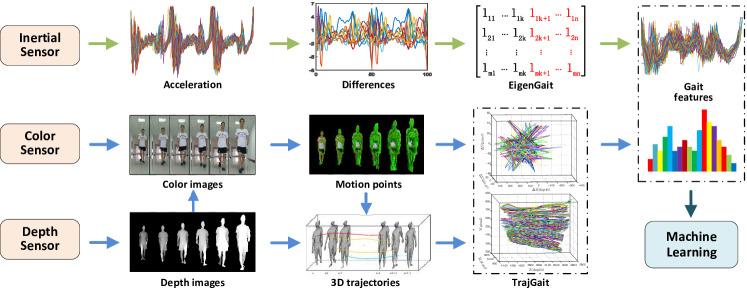
Following the application scenario of person identification shown in Fig. 1, we let the user walk straight along a corridor for gait feature collection. The inertial sensors are with the user while the color and depth sensors are placed at the end of the corridor. In this paper, we use accelerometer in the smart phone as inertial sensors and Microsoft Kinect as color and depth sensors. This way, we collect the accelerometer readings and RGBD data for gait feature extraction and gait recognition. Note that, the color (RGB) data and depth data collected by Kinect are temporally synchronized.
The flowchart of the proposed system is illustrated in Fig. 2. After data pre-processing, gait features are then extracted from the inertial data and RGBD data by using the proposed EigenGait and TrajGait algorithms, respectively. Finally, the gait features are combined as an input to the machine learning component for person identification. The proposed system can be installed at the entrance of any restricted area for person identification, such as banks, financial tower, and military base etc.
The proposed gait recognition combining multiple sensors is not fully non-invasive. The inertial sensors move with the user and send the accelerometer data to the server. Therefore, the user should be notified priorly and may need to show certain level of cooperation in data collection. But from the application perspective, most, if not all, existing person person-identification systems for accessing a restricted area cannot be fully non-invasive – many of them work as a verification system where the user needs to provide his identity to the server for verification at the entrance. For such a person-identification system, the goal is to achieve good usability instead of full non-invasiveness. For better usability, a person-identification system should require as fewer human interactions and less strict cooperations as possible. For the proposed system, with appropriate settings and client applications in each user’s smart phone, the data collection, including sending the inertial and RGBD data, and possibly the user’s identity, to the server, and the whole process are fully automatic without additional human interactions. In addition, as shown in the later experiments, by combining multiple sensors, the proposed system shows higher robustness against covariate conditions. This also improves the usability by requiring less strict cooperations from the user.
In the following, we first introduce the data collection and data pre-processing, and then elaborate on the EigenGait algorithm for inertia-based gait representation and the TrajGait algorithms for color- and depth-based gait representation.
III-B Data Collection and Pre-processing
In this paper, we use accelerometer to collect inertial data and Kinect to collect RGBD data.
III-B1 Acceleration data
We utilize a tri-axial accelerometer sensor in the smart phone to collect the acceleration data of a walking person. First, we build an application on the Android platform. Given the APIs provided by the Android SDK, we use the android.harware.SensorManager package and attached event listeners to the Sensor.Type_Accelerometer to collect acceleration data. The sensor is registered to the SensorManager.Sensor_Delay_Game and is set a sampling rate of 50Hz on each axis.
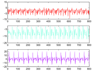
Considering the usability, in data collect we simply ask the user to put the smart phone, installed with our application, in his/her pocket with any orientation. Each user is required to walk in his/her normal pace and fast pace. Since the accelerometer is placed in the pocket with a random orientation, which varies over time during the walking, the acceleration values on each axis are collected in a time-varying direction. Therefore, the acceleration values along each axis are actually not comparable from time to time. To address this issue, we fuse the acceleration values on all three axes into one compound one. Let , and be the acceleration values on the X, Y, and Z axes, respectively, we compute the compound acceleration value by =, which is more robust against the pose change of the accelerometer over time.
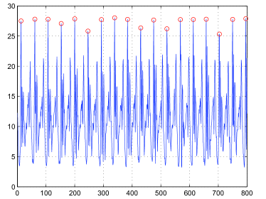
Figure 3 shows an acceleration data sample on the X, Y and Z axes collected by a smart phone – the periodical property of the acceleration data reflects the walking pace of the user. Figure 3 shows the compound acceleration curve, which has been partitioned at local maximum. Specifically, we sequentially consider a point as the partitioning point if it satisfies three conditions: 1) it is a local maximum (peak) along the curve, 2) its distance to the previous partitioning point is no less than 700ms, and 3) its value is greater than 4/.
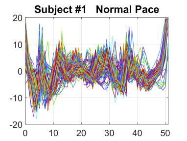
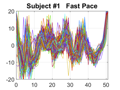
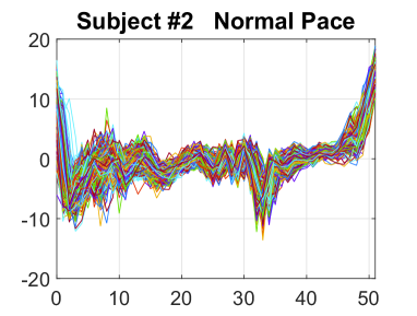
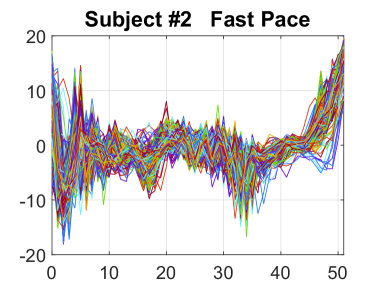
Each segment of the partitioning acceleration curve corresponds to one step in the walking. Note that, in our study, one step denotes a full step cycle consisting of a left-foot move and a right-foot move. Figures 4 (a) and (b) show 100 one-step acceleration-curve segments of an user, under normal pace and fast pace, respectively, and Figures 4 (c) and (d) show those of another user. We can see that, although the acceleration curves vary a lot between different users, the acceleration curves of the same user share similar shapes, even under different paces.
III-B2 Color and depth data
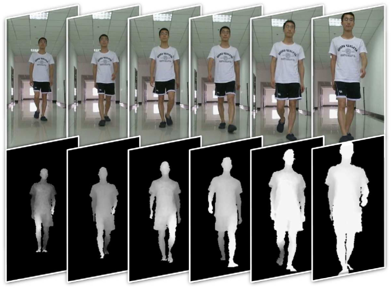

A Kinect 2.0 assisted with Kinect SDK v2.0111 http://www.microsoft.com/en-us/kinectforwindows/develop/downloads-docs.aspx is applied for color and depth data collection. The Kinect is placed about 0.5m up from the ground. The RGB video stream is in 24-bit true color format with a resolution of 12801024 pixels. The depth video stream is in VGA resolution of 640480 pixels, with 13-bit depth value. The depth sensor has a practical ranging limit of 1.2-3.5m distance when using the Kinect SDK. The sampling rate is 15 fps. Figure 5 shows a sequence of color images and depth images collected by the Kinect. The depth images shown in Fig. 5 have been normalized since a single VGA channel has only 8 bits to represent a pixel. For the computation in all the experiments, the original 13-bit depth value is used, which provides a high precision to describe the motion in the depth channel.
III-B3 Three datasets
Using the sensor settings as described above, we collect three datasets consisting of both RGBD data and accelerometer readings. We use these data for evaluating the performance of the proposed method, as well as the comparison methods, in the later experiments.
| Dataset name | Number of subjects |
|
RGBD data | Sub-datasets | Walking pace | Other information | |||||||||||||||
|---|---|---|---|---|---|---|---|---|---|---|---|---|---|---|---|---|---|---|---|---|---|
| Dataset #1 |
|
|
|
|
Normal, Fast |
|
|||||||||||||||
| Dataset #2 |
|
500 samples | 500 samples | 2-steps: 500 samples | Normal |
|
|||||||||||||||
| Dataset #3 |
|
|
|
2-steps: 2,400 samples | Normal, Fast |
|
-
Dataset #1. This dataset is collected on 10 subjects, containing 1,000 groups of acceleration data and 1000 groups of RGBD data – 100 groups of acceleration data and 100 groups of RGBD data are collected for each subject, with half in normal pace, and half in fast pace. The acceleration data and RGBD data are collected separately. In collecting acceleration data, each subject is required to walk along a hallway, with a length of about 60 feet. A group of acceleration data is defined as the sequence of acceleration values resulting from the entire walk from one end of the hallway to the other end. We partition the acceleration data into steps as illustrated in Fig. 3(b). For all the one-step acceleration data, we temporally interpolate them into a data sequence of length 50. Based on the temporally partitioning, we create 5 sub-datasets, containing one-, two-, three-, four- and five-step long data samples, respectively. In RGBD data collection, each subject is required to walk towards the Kinect 100 times, from about 5m away to 1m away to the Kinect. The sequences of frontal color and depth images of the subjects are captured. A group of RGBD data is defined as the sequence of RGBD images resulting from one full walk toward the Kinect.
-
Dataset #2. This dataset contains 500 data samples of 50 subjects, with 10 data samples for each subject. Each data sample consists of a sequence of acceleration data and a sequence of RGBD data, which are collected simultaneously for one full walk of a user. For each RGBD video, a frame is preserved only if the present person is recognized with all the body joints by the Kinect SDK. Each acceleration data covers about 2 steps or more. We uniformly partition each acceleration data and generate a two-step data sample.
-
Dataset #3. This dataset contains 2,400 data samples of 50 subjects, with 48 data samples for each subject. These data are collected under different covariate conditions. In particular, in collecting Dataset #3, each subject is required to walk under eight different conditions, i.e., natural walking, left hand in pocket, right hand in pocket, both hands in pocket, left hand holding a book, right hand holding a book, left hand with loadings, and right hand with loadings, as shown in Fig. 6. For each subject, 6 data samples are collected under each condition, with 3 in fast pace and 3 in normal pace. Acceleration data and RGBD data are collected simultaneously in each data sample. The information of the above three datasets is summarized in Table I.
III-C EigenGait: eigenspace feature extraction for gait representation
A sequence of (compound) acceleration values resulting from a walk can be plotted into a 2D curve, as illustrated in Fig. 4 and we call it a gait curve in this paper. Inspired by the Eigenface algorithm [60] used for image-based face recognition, we propose an EigenGait algorithm for gait recognition based on gait curves.
Let = = be a set of gait curves of subjects, denotes the gait curves collected for the th subject. Treating a gait curve as a vector, we can compute an average gait curve for the th subject as
| (1) |
where is the total number of gait curves collected for the th subject, and is the th gait curve of the th subject. Further, the overall average gait curve over all the subjects can be calculated by
| (2) |
Then, a gait-curve difference can be calculated by
| (3) |
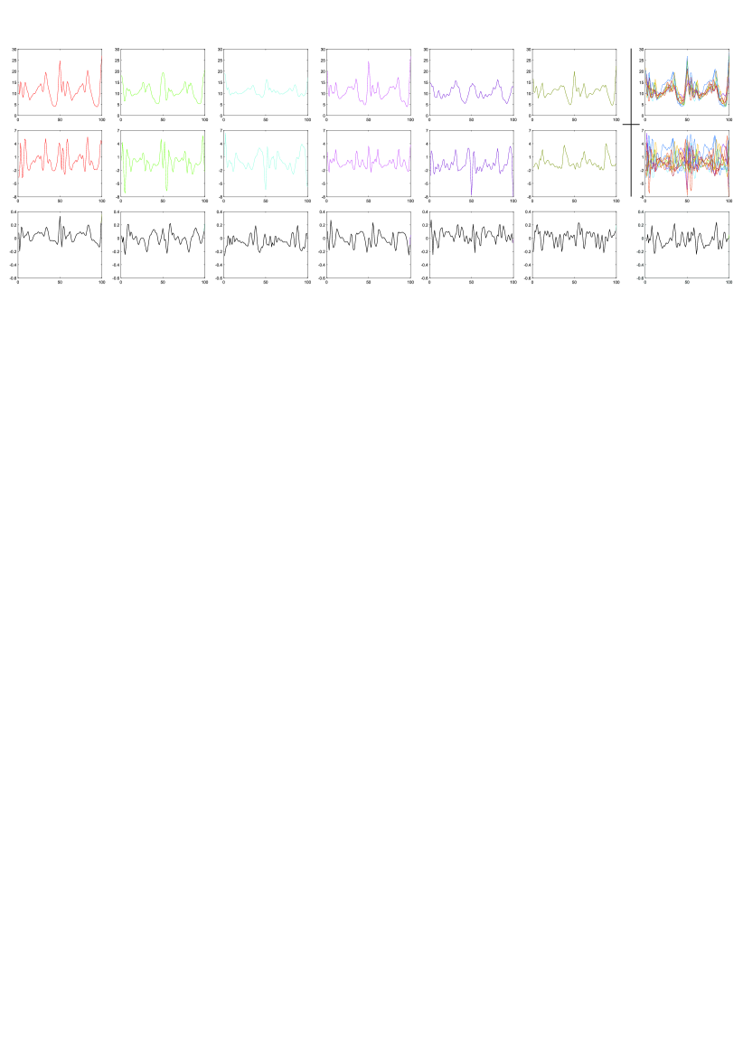
To better illustrate the meaning of , we compute them on real data. Without loss of generality, let us consider the 2-step acceleration data collected in Dataset #1. In Fig. 7, the last figure in the middle row shows the gait-curve differences of ten subjects in Dataset #1. It can be seen from Fig. 7 that, the gait-curve differences also preserve the periodic property of the original gait curve, as shown in the top row of Fig. 7, and different subjects have different gait-curve differences.
Then the covariance matrix can be calculated by
| (4) |
We can perform an eigen-decomposition as
| (5) |
where denotes the eigenvalues, and denotes the corresponding eigenvectors. Suppose the eigenvalues in have been sorted in descending order, we select the first elements that fulfill , and hence get corresponding eigenvectors . In the bottom row of Fig. 7, the seven curves show the top seven eigenvectors of the two-step sub-dataset in Dataset #1. It can be seen from Fig. 7 that, more distinctiveness can be observed in the gait-curve differences than in the original gait curves. We can also see that, these eigenvectors preserve the shape appearance of some of the original gait curves, as shown in the top row of Fig. 7 and we call them EigenGaits in this paper. When a new gait curve comes, we can project it into the eigenspace defined by the eigenvectors as
| (6) |
and obtain an EigenGait feature vector . As the acceleration data reflects the whole body motion in the walking, the extracted EigenGait features can capture the general gait dynamics.
III-D TrajGait: dense 3D trajectories based gait representation
The gait data captured by color sensor and depth sensor can be represented by a sequence of color images and depth images, respectively. These images provide useful information to describe the details of body movements, e.g., the movement of each body part. We combine the color and depth data and develop a TrajGait algorithm for extracting 3D dense trajectories and describing more detailed gait sub-dynamics.
TrajGait algorithm is summarized in Algorithm 1, which contains the following four key operations:
-
computMotion One each RGB color frame, we compute the dense optical flow by the algorithm proposed by Frneback [61]222 It is implemented and released by OpenCV 2.4.8 or above.. This algorithm makes a good compromise between accuracy and speed.
-
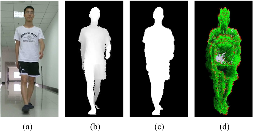
segmentMask To focus on the walking person, we segment the person from the background, and take it as a mask in later operations. Since the Kinect SDK has provided functions for efficient human detection and joints tracking [62], we apply these functions to extract a raw human mask in each frame, and then apply some image processing techniques, including hole filling and noise removal, to get the final mask. Figure 8(c) displays a human mask segmented from the depth image in Fig. 8(b). Note that, while segmenting persons from a confusing background can be very challenging on RGBD data, it is not a serious issue in the proposed application scenario of person identification – the environment is highly controlled (e.g., a hallway) and the sensors are well set, without any other moving objects around. In this paper, the following steps are taken to obtain the human mask: (i) produce human-oriented depth image using the body-segmentation function provided by Kinect SDK (i.e., IBodyIndexFrame::AccessUnderlyingBuffer), (ii) resize the depth image to the size of the color image and interpolate the resized image using bi-cubic interpolation, (iii) binarize the depth image with a threshold =113, and (iv) fill the holes and remove segments that are smaller than 1,000 pixels.
Algorithm 1 TrajGait algorithm 1:procedure TrajGait2: input:3: : RGB data collected for subjects,4: : the corresponding depth data,5: : the number of data samples in each set,6: : the number of centers in the K-means clustering,7: : the number of frames in a trajectory,8: output:9: : feature histograms for all RGBD10: videos, where .11:12: % Calculate the trajectories of all RGBD data:13: for (=1 to ) do14: for (=1 to ) do15: % Compute the motion on the color video :16: ;17: % Segment foreground (human) from the depth video:18: Mask;19: % Calculate 3D trajectories in the RGBD channel:20: Mask;21: ;22: end for23: end for24:25: % Put all trajectories together:26: ;27: % Compute a number of centers using Clustering:28: ;29:30: % Compute trajectory histogram for each RGBD data sequence:31: for (=1 to ) do32: for (=1 to ) do33: ;34: end for35: end for36:end procedure -
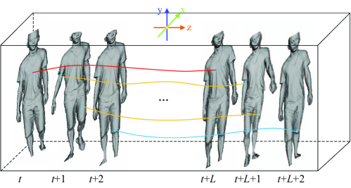
calcTrajectories Suppose is the coordinate of a point at a frame of the collected color data, is the depth value of that point in the depth video, then we can locate that point with a coordinate in the RGBD space. In this way, we can treat each point in the RGBD data as a 3D point. Figure 9 illustrates the trajectories in the 3D space. The shape of a trajectory encodes the local motion patterns, which we use for gait representation. Based on the 2D dense trajectories extracted by [63] in RGB channels, we can compute the corresponding 3D trajectories.
Let’s further suppose point at frame is tracked to frame +1 at the point , then, with a given trajectory length , we can describe its shape by a displacement vectors,
(7) where , and is empirically set as 15. Since the gait may be collected in various walking speed [64], the resulting vector has to be normalized to reduce deviations. As the metric in the color image is different from that in the depth image, we separately normalize them by their sums of the magnitudes of the displacement vectors. We take a normalized displacement vector as a 3D trajectory descriptor. An example of 3D trajectory descriptors derived from an RGBD data sequence is shown in Fig. 10.
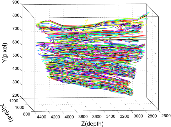
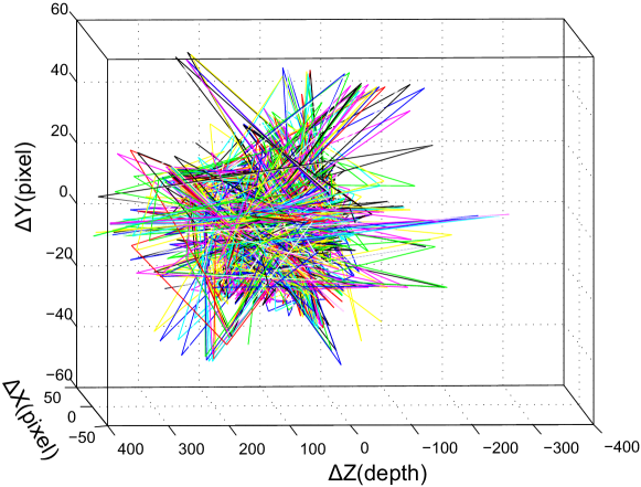
Figure 10: An example of the 3D trajectory descriptors. (a) 3D trajectories extracted from an RGBD data sequence, (b) the 3D trajectory displacements, i.e., 3D trajectory descriptors, computed on the trajectories in (a). -
histTrajectory We apply a bag-of-words strategy to encode the 3D trajectory descriptors. Specifically, we generate a codebook with a number of codes using a clustering technique. The standard K-means algorithm is employed here for clustering. To reduce the complexity, we cluster a subset of 1,000,000 randomly selected training samples. To increase the precision, we run K-means 10 times and keep the result with the lowest K-means clustering cost. For each RGBD sequence, the extracted 3D trajectory descriptors are quantized into a histogram by hard assignment. The resulting trajectory histograms are then used for gait representation.
III-E Gait Recognition
We achieve gait recognition using a supervised classifier. We combine the gait features extracted by EigenGait and TrajGait and feed them into a machine learning component for training and testing. The trained model can then be used to recognize new unseen data samples for gait recognition and person identification. For feature combination, we simply concatenate the EigenGait features and the TrajGait features into one single feature vector.
In the machine learning component, a multiclass Support Vector Machine (SVM) classifier implemented by libSVM333www.csie.ntu.edu.tw/ cjlin/libsvm/ is used for both training and testing [65]. A one-vs-all classification strategy is applied. To investigate the potential relation between classification accuracy and computation efficiency, we try both the linear and non-linear SVMs. For the soft-margin constant in SVM, we consistently set it 1,000 through all the experiments.
IV Experiments and Results
In this section, we use three datasets to evaluate the performance of the proposed method, as well as the comparison methods. First, we examine the effectiveness of the proposed EigenGait algorithm and the TrajGait algorithm using Dataset #1, separately. Then, we evaluate the performance of the proposed method, i.e., the one fusing EigenGait and TrajGait, on Dataset #2 by comparing its accuracy with several state-of-the-art gait recognition methods. Finally, we test the robustness of the proposed method on Dataset #3. In particular, we try to answer the following questions:
-
-
How effective are the EigenGait algorithm and the TrajGait algorithm for gait recognition? How do the parameters influence their performances?
-
-
What is the overall performance of the proposed method? Does it work better than the state-of-the-art color-based methods, depth-based methods, and inertia-based methods?
-
-
How robust is the proposed method in handling gait data collected under hard-covariate conditions?
In the experiments, we mainly evaluate gait recognition to address a classification problem. At the end of the section, we will also evaluate the proposed method to solve an identification problem. As a classification problem, we use the classification accuracy as a metric for performance evaluation. The classification accuracy is defined as
| (8) |
In the classification, each testing sample is classified by the pre-trained SVM and receives a score vector containing score values, where is the number of subjects in training the SVM. A score value in the score vector indicates the likelihood of this sample to be from a specific subject. The sample will be recognized as being from subject if the th element is the maximum in the score vector. Compared with the ground-truth subject for the test sample, we can decide whether it is correctly classified and compute the accuracy.
| Walking pace | Kernel | 1 step | 2 steps | 3 steps | 4 steps | 5 steps | 6 steps | 7 steps | 8 steps |
|---|---|---|---|---|---|---|---|---|---|
| Normal | KL1 | 0.9616 | 0.9616 | 0.9608 | 0.9659 | 0.9634 | 0.9626 | 0.9525 | 0.9606 |
| KCHI2 | 0.9522 | 0.9510 | 0.9471 | 0.9520 | 0.9449 | 0.9454 | 0.9393 | 0.9354 | |
| Fast | KL1 | 0.8948 | 0.9308 | 0.9515 | 0.9398 | 0.9467 | 0.9437 | 0.9387 | 0.9250 |
| KCHI2 | 0.8894 | 0.9208 | 0.9433 | 0.9292 | 0.9356 | 0.9244 | 0.9200 | 0.9018 | |
| Normal&Fast | KL1 | 0.8790 | 0.9048 | 0.9242 | 0.9183 | 0.9213 | 0.9247 | 0.9094 | 0.8977 |
| KCHI2 | 0.8785 | 0.8992 | 0.9156 | 0.9082 | 0.9219 | 0.9054 | 0.8913 | 0.8900 |
IV-A Effectiveness
We use Dataset #1 to evaluate the performance of the EigenGait algorithm and the TrajGait algorithm. Dataset #1 is collected for 10 subjects, including five sub-datasets of the acceleration data, and one sub-dataset of the RGBD data.
IV-A1 EigenGait
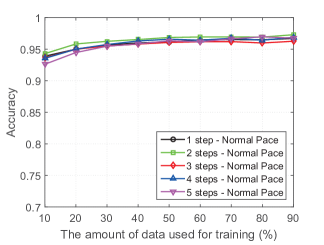
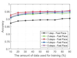
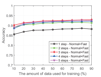
There are five acceleration sub-datasets, i.e., the one-, two-, three-, four- and five-step sub-datasets. Each sub-dataset contains 5,000 acceleration data sequences, with half in normal pace and half in fast pace. The resulting EigenGait features are of dimension 43, 85, 128, 170 and 213 for the one-, two-, three-, four- and five-step data, respectively. Note that, data in the same sub-dataset have no overlaps with each other. The EigenGait algorithm is evaluated under the normal pace, fast pace and two paces mixed, i.e., normal+fast, and the results are shown in Fig. 11(a)-(c), respectively. From Fig. 11(a)-(c), we can see that, EigenGait obtains good classification accuracy in all three cases, e.g., over 0.95 in normal pace, 0.92 in fast pace, and 0.90 in normal+fast, using 30% data for training. Moreover, EigenGait shows higher accuracy under normal pace than under fast pace. This is because, a large speed variation would occur when a person walks in a fast pace, which would increase the complexity of the gait data. Decreased performances of EigenGait can be observed in Fig. 11(c), because the mixed-pace data further increase the data complexity.
As can be seen from Fig. 11(b) and (c), on a dataset with large speed variations, e.g., in fast pace, or in normal+fast, EigenGait holds lower performances on the 1-step dataset than on two or more step dataset. This is because, a 1-step data is less capable of representing the gait than a 2 or more step data. Surprisingly, the EigenGait obtains comparable performances when varying the data length from 2 to 5 steps. Considering that a 2-step data can be easily captured and efficiently computed as comparing to longer data, in our later experiments, we always choose a length of 2 steps for EigenGait features, including the experiments on Dataset #2 and Dataset #3.
Further, we evaluate EigenGait’s performance using linear and non-linear SVMs. Typically, the ‘KL1’ and ‘KCHI2’ kernels are employed, respectively. Table II lists the classification accuracy under different walking paces and varied data lengths, where 50% data are used for training. It can be seen that, EigenGait generally shows higher performances using a linear SVM than using a non-linear one. This is because, the EigenGait extracts gait features in the eigenspace, which makes the feature more linearly classifiable.
IV-A2 TrajGait
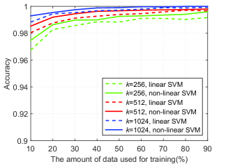
We use RGBD data in Dataset #1 to evaluate the TrajGait algorithm. Specifically, we evaluate the TrajGait under different for K-means clustering, and linear and non-linear SVMs. In K-means clustering, 1,000 trajectories are randomly selected for each training sample. In feature quantization, all trajectories of each data sample are used, which may span from about 8,000 to 15,000 in our experiments. Figure 11(d) shows the TrajGait accuracy when =256, 512 and 1024., respectively. We can see that the TrajGait achieves classification accuracies higher than 0.98 when using over 20% data for training. A higher performance can be achieved with a larger , i.e., the size of the codebook. It can also be observed that, under the same , a non-linear SVM produces a little higher accuracies than the linear one. Considering that linear SVM performs better in EigenGait and has lower computation cost, we choose the linear SVM in the proposed gait recognition by combining the EigenGait and TrajGait features.
IV-B Accuracy
We evaluate the overall performance of the proposed method, i.e., EigenGait+TrajGait, by comparing it with several other inertia-based methods, color and depth based methods. Specifically, the following methods are included in the comparison,
-
Acc_Fourier [21]: An autocorrelation operation is first applied to the acceleration data, which is then converted into the frequency domain using FFT. The top half of the coefficients are selected as the gait features.
-
Acc_Wavelet [18]: The Mexican Hat Wavelet transform is used to analyze the gait patterns from the acceleration data.
-
Acc_EigenGait: The proposed EigenGait algorithm handles the acceleration data.
-
D_Skeleton [42]: The position matrix on 20 joints are decomposed by SVD, and the resulting 220-dimensional vectors are used for gait representation.
-
D_GEV [12]: The GEV is computed on the human masks extracted from depth data. The principal component analysis is then performed the same way as in our EigenGait for gait features.
-
D_TrajGait: The displacement of a trajectory is calculated only on the depth channel, with a codebook size =1024.
-
RGB_TrajGait: The displacement of a trajectory is calculated on the RGB channels, with =1024.
-
RGBD_TrajGait: The full TrajGait algorithm, i.e., trajectories extracted from the RGBD channels, with =1024.
-
Acc_EigenGait+RGBD_TrajGait: The full version of the proposed method by combining EigenGait and TrajGait features. We normalize the EigenGait feature and TrajGait feature independently before concatenating them together. Afterwards, we normalize the concatenated feature as an input data for SVM. The normalization is performed using an L1-norm measure.
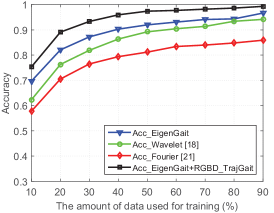
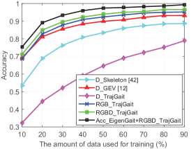
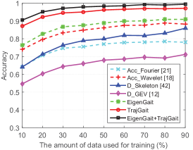
For clarity, we use Figs. 12(a) and (b) to show the results of the acceleration-based methods and the RGBD-based methods, respectively. In Fig. 12(a), the proposed EigenGait is observed with a clear higher performance than the wavelet-based or FFT-based methods, in handling acceleration data. In Fig. 12(b) we can see that, RGBD_TrajGait obtains an accuracy over 0.90 when using 30% data for training, which is much higher than that of D_Skeleton and D_GEV. The TrajGait has a higher performance on the RGB channels than on the depth channel, which indicates that the color is more effective than the depth in representing gait sub-dynamics. Meanwhile, RGBD_TrajGait outperforms RGB_TrajGait and D_TrajGait, which simply demonstrates that the color information and depth information can complement each other in characterizing the gait. It can also be seen from Fig. 12(b) that, a boosted performance can be achieved by fusing EigenGait (handling acceleration data) and TrajGait (handling RGBD data) features, i.e., EigenGait+TrajGait, which validates the effectiveness of the proposed multi-sensor data fusion strategy.
IV-C Robustness
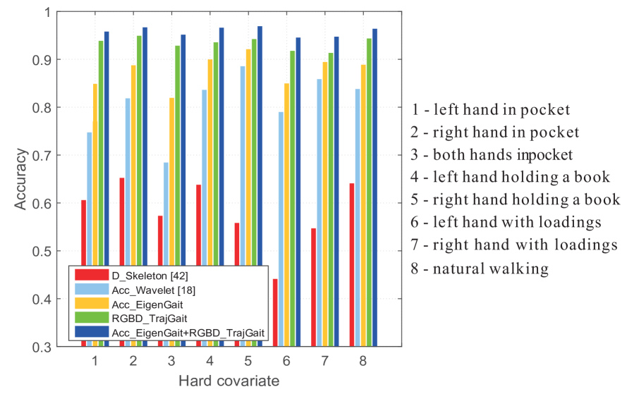
We evaluate the robustness of the proposed method with Dataset #3, which contains 2,400 data samples of 50 subjects, under 8 hard-covariate conditions, as introduced in Section III-B3. Figure 12(c) shows the results of the proposed method and the comparison methods. We can see that, the TrajGait+EigenGait, the TrajGait, and the EigenGait achieves the top three performances among all the methods. The proposed method, i.e., TrajGait+EigenGait, stably hold an classification accuracy over 0.90 when varying the amount of training data from 10% to 90%, which indicates the proposed method can better handle these hard covariates.
Moreover, we investigate the detailed performance of the proposed method by figuring out the classification accuracies on each kind of hard covariate. As shown in Fig. 13, for EigenGait, the hard covariate ‘both hands in pocket’ leads to the lowest accuracy. It is because that, the acceleration would heavily vary from normal when a person walks with both hands in the pockets. While for TrajGait, ‘a hand with loadings’ will increase the difficulty for gait recognition. This is because the loadings may bring unexpected motions in the color space, as well as in the depth space, e.g., a bag is used to carry the loadings in our case. For the skeleton-based and wavelet-based methods, the average classification accuracy is about 30% and 10% lower than the proposed method, respectively. Comparing with the turbulent performances of the comparison methods on different hard covariates, the proposed method performs rather stably.
IV-D Person-Identification Performance
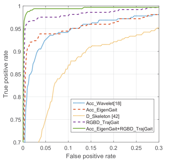
Finally, we evaluate the proposed method in the application scenario of person identification, as shown in Fig. 1. Half of the data samples in Dataset #3 are used for training, and the remaining half are used for querying and identification. The average ROC curve [66, 67] is employed for performance evaluation. For each subject, an ROC curve is computed on the results of a one-vs-all binary classification. The ROC curve is created by plotting the true positive rate (TPR) against the false positive rate (FPR) at varying threshold settings. The TPR and FPR are defined by
| (9) |
| (10) |
Then the average ROC curve is computed based on all ROC curves of 50 subjects. The larger the area under the ROC curve, the better the person-identification performance. The average ROC curves for the proposed method and the comparison methods are plotted in Fig. 14. We can see that, the proposed method by combining EigenGait and TrajGait achieves the best performance. In addition, the EigenGait and the Wavelet-based method produce competing performance, but the former achieves higher TPR than the later when the FPR is below 0.05. Thus, the EigenGait would outperform the Wavelet-based method since a lower FPR is often required in a strict identification system. It can also be observed from Fig. 14 that, the TrajGait uniformly outperforms the EigenGait which may simply indicate that the TrajGait features are more discriminative by describing the detailed gait sub-dynamics.
V Conclusion
In this paper, the inertia, color and depth sensors were integrated for accurate gait recognition and robust person identification. Specifically, the accelerometer of smart phone and the RGBD sensor of Kinect were employed for data collection. An EigenGait algorithm was proposed to process the acceleration data from inertial sensor in the eigenspace, and capture the general dynamics of the gait. A TrajGait algorithm was proposed to extract gait features on the dense 3D trajectories from the RGBD data, and capture the more detailed sub-dynamics. The extracted general dynamics and detailed sub-dynamics were fused and fed into a linear SVM for training and testing. Datasets collected from 50 subjects were used for experiments and the results showed the effectiveness of the proposed method against several existing state-of-the-art gait recognition methods.
In the experiments, there are several other interesting findings. First, for the acceleration-based gait recognition, the walking pace has a potential influence on accuracy of the system. Uniform walking pace under a normal speed produces better gait recognition than mixed walking paces. Second, for the RGBD-based gait recognition, motion can be better captured by wearing textured clothes, with which we can more accurately infer the detailed gait sub-dynamics for gait recognition. Third, the proposed construction and encoding of the 3D dense trajectories can provide more discriminative and robust gait features under different hard-covariate conditions than other sparse joint-based trajectories.
In the future, we plan to further enhance the gait recognition system by configuring more sensors and building more effective classifiers. For example, more Kinects may be installed to capture multiple views of a walking person. For the classifier, other proved techniques in classification, such as the fuzzy-reasoning strategies [68, 69, 70] may be integrated into SVM to improve the recognition accuracy and robustness.
References
- [1] M. Nixon, T. Tan, and R. Chellapppa, “Human identification based on gait,” Springer Science + Business Media Inc., 2006, ch. 1.
- [2] J. Zhang, J. Pu, C. Chen, and R. Fleischer, “Low-resolution gait recognition,” IEEE Transactions on Systems, Man, and Cybernetics, Part B: Cybernetics, vol. 40, no. 4, pp. 986–996, 2010.
- [3] M. Ding and G. Fan, “Multilayer joint gait-pose manifolds for human gait motion modeling,” IEEE Transactions on Cybernetics, vol. 45, no. 11, pp. 2413–2424, 2015.
- [4] A. Kale, A. Rajagopalan, N. Cuntoor, and V. Krueger, “Gait-based recognition of humans using continuous HMMs,” in International Conference on Automatic Face and Gesture Recognition, 2002, pp. 336–341.
- [5] J. Han and B. Bhanu, “Individual recognition using gait energy image,” in IEEE Conference on Computer Vision and Pattern Recognition, 2003, pp. 1–8.
- [6] Z. Liu and S. Sarkar, “Improved gait recognition by gait dynamics normalization,” IEEE Transactions on Pattern Analysis and Machine Intelligence, vol. 28, no. 6, pp. 863–876, 2006.
- [7] Y. Ran, Q. Zheng, R. Chellappa, and T. M. Strat, “Applications of a simple characterization of human gait in surveillance,” IEEE Transactions on Systems, Man, and Cybernetics, Part B: Cybernetics, vol. 40, no. 4, pp. 1009–1020, 2010.
- [8] J. Gu, X. Ding, S. Wang, and Y. Wu, “Action and gait recognition from recovered 3-d human joints,” IEEE Transactions on Systems, Man, and Cybernetics, Part B: Cybernetics, vol. 40, no. 4, pp. 1021–1033, 2010.
- [9] W. Kusakunniran, Q. Wu, J. Zhang, Y. Ma, and H. Li, “A new view-invariant feature for cross-view gait recognition,” IEEE Transactions on Information Forensics and Security, vol. 8, no. 10, pp. 1642–1653, 2013.
- [10] N. Boulgouris and X. Huang, “Gait recognition using HMMs and dual discriminative observations for sub-dynamics analysis,” IEEE Transactions on Image Processing, vol. 22, no. 9, pp. 3636–3647, 2013.
- [11] M. Goffredo, I. Bouchrika, J. N. Carter, and M. S. Nixon, “Self-calibrating view-invariant gait biometrics,” IEEE Transactions on Systems, Man, and Cybernetics, Part B: Cybernetics, vol. 40, no. 4, pp. 997–1008, 2010.
- [12] S. Sivapalan, D. Chen, S. Denman, S. Sridharan, and C. Fookes, “Gait energy volumes and frontal gait recognition using depth images,” in International Joint Conference on Biometrics, 2011.
- [13] V. John, G. Englebienne, and B. Krose, “Person re-identification using height-based gait in colour depth camera,” in International Conference on Image Processing, 2013, pp. 3345–3349.
- [14] P. Chattopadhyay, A. Roy, S. Sural, and J. Mukhopadhyay, “Pose depth volume extraction from rgb-d streams for frontal gait recognition,” Journal of Visual Communication and Image Representation, vol. 25, no. 1, pp. 53–63, 2014.
- [15] J. Mantyjarvi, M. Lindholm, E. Vildjiounaite, S. Makela, and H. Ailisto, “Identifying users of portable devices from gait pattern with accelerometers,” in IEEE Conference on Acoustics, Speech, and Signal Processing, 2005, pp. 973–976.
- [16] R. Liu, Z. Duan, J. Zhou, and M. Liu, “Identification of individual walking patterns using gait acceleration,” in International Conference on Bioinformatics and Biomedical Engineering, 2007, pp. 543–546.
- [17] J. Kwapisz, G. Weiss, and S. Moore, “Cell phone-based biometric identification,” in International Conference on Biometrics: Theory Applications and Systems, 2010, pp. 1–7.
- [18] F. Xu, C. Bhagavatula, A. Jaech, U. Prasad, and M. Savvides, “Gait-ID on the move: Pace independent human identification using cell phone accelerometer dynamics,” in International Conference on Biometrics: Theory Applications and Systems, 2012, pp. 8–15.
- [19] N. Trung, Y. Makihara, H. Nagahara, R. Sagawa, Y. Mukaigawa, and Y. Yagi, “Phase registration in a gallery improving gait authentication,” in International Joint Conference on Biometrics, 2011.
- [20] N. Trung, Y. Makihara, H. Nagahara, Y. Mukaigawa, and Y. Yagi, “Performance evaluation of gait recognition using the largest inertial sensor-based gait database,” in IAPR International Conference on Biometrics, 2012, pp. 360–366.
- [21] B. Sun, Y. Wang, and J. Banda, “Gait characteristic analysis and identification based on the iPhone’s accelerometer and gyrometer,” Sensors, vol. 14, no. 9, pp. 17 037–17 054, 2014.
- [22] J. Cutting and L. Kozlowski, “Recognition of friends by their walk,” Bulletin of the Psychonomic Society, vol. 9, pp. 353–356, 1977.
- [23] A. M. de-la Herran, B. Garcia-Zapirain, and A. Mendez-Zorrilla, “Gait analysis methods: an overview of wearable and non-wearable systems, highlighting clinical applications,” Sensors, vol. 14, no. 2, pp. 3362–3394, 2014.
- [24] C. BenAbdelkader, R. Cutler, and L. Davis, “Stride and cadence as a biometric in automatic person identification and verification,” in International Conference on Automatic Face and Gesture Recognition, 2002, pp. 372–377.
- [25] L. Wang, T. Tan, H. Ning, and W. Hu, “Silhouette analysis based gait recognition for human identification,” IEEE Transactions on Pattern Analysis and Machine Intelligence, vol. 25, no. 12, pp. 1505–1518, 2003.
- [26] A. Kale, A. Sundaresan, A. Rajagopalan, N. Cuntoor, A. Roy-Chowdhury, V. Kruger, and R. Chellappa, “Identification of humans using gait,” IEEE Transactions on Image Processing, vol. 13, no. 9, pp. 1163–1173, 2004.
- [27] D. Tao, X. Li, X. Wu, and S. Maybank, “General tensor discriminant analysis and gabor features for gait recognition,” IEEE Transactions on Pattern Analysis and Machine Intelligence, vol. 29, no. 10, pp. 1700–1715, 2007.
- [28] L. Wang, H. Z. Ning, T. N. Tan, and W. M. Hu, “Fusion of static and dynamic body biometrics for gait recognition,” in International Conference on Computer Vision, 2003, pp. 1449–1454.
- [29] D. Tolliver and R. Collins, “Gait shape estimation for identification,” in Audio- and Video-Based Biometric Person Authentication, 2003, pp. 734–742.
- [30] J. Han and B. Bhanu, “Statistical feature fusion for gait-based human recognition,” in IEEE Conference on Computer Vision and Pattern Recognition, 2004, pp. 842–847.
- [31] Z. Zhang and N. Troje, “View-independent person identification from human gait,” Neurocomputing, vol. 69, no. 1-3, pp. 250–256, 2005.
- [32] C. BenAbdelkader, R. Culter, H. Nanda, and L. Davis, “Eigengait: Motion-based recognition people using image self-similarity,” in International Conference on Audio and Video-based Person Authentication, 2001, pp. 284–294.
- [33] C. Chen, J. Liang, and X. Zhu, “Gait recognition based on improved dynamic bayesian networks,” Pattern Recognition, vol. 44, no. 4, pp. 988–995, 2011.
- [34] I. Venkat and P. De Wilde, “Robust gait recognition by learning and exploiting sub-gait characteristics,” International Journal of Computer Vision, vol. 91, no. 1, pp. 7–23, 2011.
- [35] M. Hu, Y. Wang, Z. Zhang, D. Zhang, and J. Little, “Incremental learning for video-based gait recognition with LBP flow,” IEEE Transactions on Cybernetics, vol. 43, no. 1, pp. 77–89, 2013.
- [36] T. H. Lam, K. H. Cheung, and J. N. Liu, “Gait flow image: A silhouette-based gait representation for human identification,” Pattern recognition, vol. 44, no. 4, pp. 973–987, 2011.
- [37] F. Castro, M. Marin-Jimenez, and R. Medina-Carnicer, “Pyramidal fisher motion for multiview gait recognition,” in International Conference on Pattern Recognition, 2014, pp. 1–4.
- [38] W. Kusakunniran, “Attribute-based learning for gait recognition using spatio-temporal interest points,” Image and Vision Computing, vol. 32, no. 12, pp. 1117–1126, 2014.
- [39] C. Yam, M. S. Nixon, and J. N. Carter, “Gait recognition by walking and running: a model-based approach,” in Proceeding of the Asian Conference on Computer Vision, 2002.
- [40] D. Cunado, M. S. Nixon, and J. N. Carter, “Automatic extraction and description of human gait models for recognition purposes,” Computer Vision and Image Understanding, vol. 90, no. 1, pp. 1–41, 2003.
- [41] P. F. Felzenszwalb, R. B. Girshick, D. McAllester, and D. Ramanan, “Object detection with discriminatively trained part-based models,” IEEE Transactions on Pattern Analysis and Machine Intelligence, vol. 32, no. 9, pp. 1627–1645, 2010.
- [42] B. Munsell, A. Temlyakov, C. Qu, and S. Wang, “Person identification using full-body motion and anthropometric biometrics from kinect videos,” in European Conference on Computer Vision Workshop, 2012, pp. 91–100.
- [43] M. Gabel, R. Gilad-Bachrach, E. Renshaw, and A. Schuster, “Full body gait analysis with kinect,” in International Conference of the IEEE Engineering in Medicine and Biology Society, 2012, pp. 1964–1967.
- [44] L. Igual, A. Lapedriza, and R. Borras, “Robust gait-based gender classification using depth cameras,” EURASIP Journal on Image and Video Processing, pp. 1–11, 2013.
- [45] P. Chattopadhyay, S. Sural, and J. Mukherjee, “Frontal gait recognition from incomplete sequences using rgb-d camera,” IEEE Transactions on Information Forensics and Security, vol. 9, no. 11, pp. 1843–1856, 2014.
- [46] M. Derawi, P. Bours, and K. Holien, “Improved cycle detection for accelerometer based gait authentication,” in International Conference on Intelligent Information Hiding and Multimedia Signal Processing, 2010, pp. 312–317.
- [47] D. Gafurov, E. Snekkenes, and P. Bours, “Improved gait recognition performance using cycle matching,” in International Conference on Advanced Information Networking and Applications, 2010, pp. 836–841.
- [48] H. Chan, H. Zheng, H. Wang, R. Gawley, M. Yang, and R. Sterritt, “Feasibility study on iphone accelerometer for gait detection,” in International Conference on Pervasive Computing Technologies for Healthcare(PervasiveHealth), 2011, pp. 184–187.
- [49] T. Ngo, Y. Makihara, H. Nagahara, Y. Mukaigawa, and Y. Yagi, “The largest inertial sensor-based gait database and performance evaluation of gait-based personal authentication,” Pattern Recognition, vol. 47, no. 1, pp. 228–237, 2014.
- [50] Y. Zhang, G. Pan, K. Jia, M. Lu, Y. Wang, and Z. Wu, “Accelerometer-based gait recognition by sparse representation of signature points with clusters,” IEEE Transactions on Cybernetics, vol. 45, no. 9, pp. 1864–1875, 2015.
- [51] T. Kobayashi and N. Otsu, “Action and simultaneous multiple-person identification using cubic higher-order local auto-correlation,” in International Conference on Pattern Recognition, 2004, pp. 741–744.
- [52] N. Gkalelis, A. Tefas, and I. Pitas, “Human identification from human movements,” in IEEE International Conference on Image Processing, 2009, pp. 2585–2588.
- [53] A. Iosifidis, A. Tefas, and I. Pitas, “Activity-based person identification using fuzzy representation and discriminant learning,” IEEE Transactions on Information Forensics and Security, vol. 7, no. 2, pp. 530–542, 2012.
- [54] A. Iosifidis, A. Tefas, and I. Pitas, “Person identification from actions based on dynemes and discriminant learning,” in IEEE International Workshop on Biometrics and Forensics, 2013, pp. 1–4.
- [55] J. Lu, J. Hu, X. Zhou, and Y. Shang, “Activity-based person identification using sparse coding and discriminative metric learning,” in ACM international conference on Multimedia, 2012, pp. 1061–1064.
- [56] H. Yan, J. Lu, and X. Zhou, “Activity-based person identification using discriminative sparse projections and orthogonal ensemble metric learning,” in European Conference on Computer Vision Workshops, 2014, pp. 809–824.
- [57] H. Yan, “Discriminative sparse projections for activity-based person recognition,” Neurocomputing, 2016.
- [58] J. Wu, J. Konrad, and P. Ishwar, “The value of multiple viewpoints in gesture-based user authentication,” in IEEE Conference on Computer Vision and Pattern Recognition Workshops, 2014, pp. 90–97.
- [59] I. Kviatkovsky, I. Shimshoni, and E. Rivlin, “Person identification from action styles,” in IEEE Conference on Computer Vision and Pattern Recognition Workshops, 2015, pp. 84–92.
- [60] M. Turk and A. Pentland, “Eigenfaces for recognition,” Journal of cognitive neuroscience, vol. 3, no. 1, pp. 71–86, 1991.
- [61] G. Farnebäck, “Two-frame motion estimation based on polynomial expansion,” in Image Analysis. Springer, 2003, pp. 363–370.
- [62] J. Shotton, R. Girshick, A. Fitzgibbon, T. Sharp, M. Cook, M. Finocchio, R. Moore, P. Kohli, A. Criminisi, A. Kipman, and A. Blake, “Efficient human pose estimation from single depth images,” IEEE Transactions on Pattern Analysis and Machine Intelligence, vol. 35, no. 12, pp. 2821–2840, 2012.
- [63] H. Wang, A. Kläser, C. Schmid, and C.-L. Liu, “Action recognition by dense trajectories,” in IEEE Conference on Computer Vision and Pattern Recognition, 2011, pp. 3169–3176.
- [64] W. Kusakunniran, Q. Wu, J. Zhang, and H. Li, “Gait recognition across various walking speeds using higher order shape configuration based on a differential composition model,” IEEE Transactions on Systems, Man, and Cybernetics, Part B: Cybernetics, vol. 42, pp. 1654–1668, 2012.
- [65] C. C. Chang and C. J. Lin, “LIBSVM: a library for support vector machines,” ACM Transactions on Intelligent Systems and Technology, vol. 2, pp. 27:1–27:27, 2011.
- [66] T. Fawcett, “An introduction to roc analysis,” Pattern recognition letters, vol. 27, no. 8, pp. 861–874, 2006.
- [67] Q. Zou, Y. Cao, Q. Li, C. Huang, and S. Wang, “Chronological classification of ancient paintings using appearance and shape features,” Pattern Recognition Letters, vol. 49, pp. 146–154, 2014.
- [68] Q. Liang and J. M. Mendel, “Interval type-2 fuzzy logic systems: theory and design,” IEEE Transactions on Fuzzy Systems, vol. 8, no. 5, pp. 535–550, 2000.
- [69] H. Li, Y. Gao, P. Shi, and H.-K. Lam, “Observer-based fault detection for nonlinear systems with sensor fault and limited communication capacity,” IEEE Transactions on Automatic Control, 2015.
- [70] H. Li, C. Wu, S. Yin, and H.-K. Lam, “Observer-based fuzzy control for nonlinear networked systems under unmeasurable premise variables,” IEEE Transactions on Fuzzy Systems, 2015.