Understanding the Non-Convergence of Agricultural Futures via Stochastic Storage Costs and Timing Options

Abstract

This paper studies the market phenomenon of non-convergence between futures and spot prices in the grains market. We postulate that the positive basis observed at maturity stems from the futures holder’s timing options to exercise the shipping certificate delivery item and subsequently liquidate the physical grain. In our proposed approach, we incorporate stochastic spot price and storage cost, and solve an optimal double stopping problem to give the optimal strategies to exercise and liquidate the grain. Our new models for stochastic storage rates lead to explicit no-arbitrage prices for the shipping certificate and associated futures contract. We calibrate our models to empirical futures data during the periods of observed non-convergence, and illustrate the premium generated by the shipping certificate.

Keywords:  Optimal multiple stopping, storage cost, agricultural futures, mean reversion, non-convergence, basis
JEL Classification:  C41, D53, G13
Mathematics Subject Classification (2010):  60G40, 62L15, 91G20, 91G80

1 Introduction

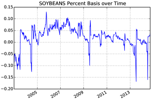
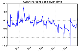
Standard no-arbitrage pricing theory asserts that spot and futures prices must converge at expiration. Nevertheless, during 2004-2009 traders observed significantly higher expiring futures prices for corn, wheat, and soybeans on the CBOT compared to the spot price of the physical grains. As shown in Figure 1, the unprecedented differential between cash and futures prices reached its apex in 2006, where at the height of the phenomenon, CBOT corn futures had surpassed spot corn prices by almost 30%! In the literature, Adjemian et al. (2013) and Aulerich et al. (2011) reported that on July 1, 2008, the price for a July 2008 CBOT wheat futures contract closed at $8.50 per bushel. On the other hand, the corresponding cash price in the Toledo, Ohio delivery market was only $7.18 per bushel, a price differential of $1.32/bu (+15%). Irwin et al. (2009) first coined the term “non-convergence” for this phenomenon of observed positive premium, which recurred persistently from 2004 onwards. According to their study, “performance has been consistently weakest in wheat, with futures prices at times exceeding delivery location cash prices by $1.00/bu, a level of disconnect between cash and futures not previously experienced in grain markets.”

However, a small difference between expiring futures and cash prices does not necessarily imply a market failure. Before expiration, futures and cash prices may differ due to the convenience yield, storage costs, or financing costs. Upon expiration, if cash prices are lower/higher than futures prices, then arbitrageurs may profit from trading simultaneously in the spot and futures markets. If sufficient numbers of arbitrageurs engage in these trades, they will drive cash and futures prices to convergence at expiration. In fact, the futures expiration date and delivery date may also differ. After the last trade date, the exchange contacts the longest outstanding long who is notified of his obligation to undertake delivery. Before the month’s end, the delivery instrument is then exchanged at the settlement price between long and short parties. Therefore, since the delivery process does not occur immediately after the last trade date, cash and futures prices might still differ by a spread called the basis. In this paper, we use the following definition for the basis:

$$\text{basis = futures price - spot price}.$$

Figure 1 displays the basis time series associated with the expiring futures on soybeans and corn.

Since the short party may choose the location and time to deliver, Biagini and Bjork (2007) posit that futures price should be biased below the spot price on the last trade date. However, their theoretical model would yield the opposite of the empirical observations in the grain markets. In fact, the positive basis in the CBOT grain markets between 2004-2009 were too large to have been caused by the small inefficiencies of the delivery process. This motivates us to investigate the factors that drive the non-convergence phenomenon.

Figure 1: Time series of basis for soybeans (left) and corn (right) futures. During 2004-2009, the expiring futures price tends to be significantly higher than the spot price.

In order to explain the positive premium, one must turn to embedded $long$-$side$ options in the futures. Long-side options in futures markets depend totally on the idiosyncrasies of each commodity’s exchange traded structure. The survey paper by Carmona and Coulon (2013) demonstrates the appropriate model for a commodity varies highly depending on storability, instantaneous utility, and alternatives. At expiration, a CBOT agricultural futures contract does not deliver the physical grains but an artificial instrument called the shipping certificate that entitles its holder to demand loading of the grains from a warehouse at any time. Before exercising the option to load, the holder must pay a fixed storage fee to the storage company, as stipulated in the certificate. Since the storage capacity of grain elevators is limited and expensive, the number of grain elevators is fixed to a minimum necessary to efficiently carry out transfers of grain from one transport system to another. Thus, like a fractional-reserve banking system, shipping certificates alleviate the congestion of grain elevators by only keeping enough grain on hand to satisfy instant withdrawal demand. A detailed explanation on the structure of the shipping certificate market can be found in Aulerich et al. (2011) and Garcia et al. (2014).

In this paper, our storage differential hypothesis posits that when the certificate storage rate is sufficiently low, investors will pay a premium for the certificate over the spot grain in order to save on storage cost over time, resulting in non-convergence of futures and spot prices. When the storage cost of the certificate is set lower than the true storage cost paid by the regular firm, the regular firm will cease to issue the unprofitable shipping certificates. Since shipping certificates can only be issued by a set number of regular firms with limited inventories, the market cannot issue certificates with lower fixed storage rates to keep the market flowing. Instead, since the supply of certificates remains fixed, the value of existing shipping certificates will be bid up in the secondary market, resulting in a premium over the spot price. On the other hand, during periods where the certificate storage rate is set much higher than the market storage rate, the certificate should not command any premium over the spot because agents would exercise and store at the lower market rate. Therefore, as shown by Aulerich et al. (2011), large quantities of certificates remaining unredeemed under the storage differential hypothesis becomes a strong predictor of non-convergence. In fact, in 2009 under mounting evidence that storage differentials were responsible for non-convergence, the CBOT raised the certificate storage rate for wheat, after which non-convergence decreased significantly. This observation is consistent with our findings in this paper.

Let us point out an alternative explanation for non-convergence even though it is not the approach in this paper. The speculator hypothesis for non-convergence postulates that large $long$ positions held by commodity index traders (CITs) have made it impossible for arbitrageurs to carry sufficient grain forward to drive terminal prices to convergence (see Tang and Xiong (2012) an example of the effects of excess speculation). While the speculator hypothesis is plausible, empirical studies by Garcia et al. (2014) and Irwin et al. (2011) found no evidence that rolling or initiation of large positions by index funds had contributed to an expansion of the basis. In this paper, we illustrate mathematically how the non-convergence phenomenon can arise under rational no-arbitrage models with stochastic storage rates.

We propose two new models that incorporate the stochasticity of the market storage rate and capture the storage option of the shipping certificate by solving two optimal timing problems, namely, to exercise the shipping certificate and subsequently liquidate the physical grain. First, we propose the Martingale Model whereby the spot price minus storage cost is a martingale while the stochastic storage rate follows an Ornstein-Uhlenbeck (OU) process. In addition, we present a second model in which the stochastic storage rate is a deterministic function of the spot price that follows an exponential OU (XOU) process. Among our results, we provide explicit prices for the shipping certificate, futures prices, and the basis size under a two continuous-time no-arbitrage pricing models with stochastic storage rates. By examining the divergence between expiring futures prices and corresponding spot prices, we derive the timing option generated by the differential between the market storage rate and the constant storage rate stipulated in the shipping certificate, which explains the non-convergence phenomenon in agricultural commodity markets. We also fit our model prices to market data and extract the numerical value of the embedded timing option.

The rest of the paper is organized as follows. Section 2 reviews the literature on the subject of non-convergence for agricultural futures. In Section 3, we discuss a martingale spot price model with an OU stochastic storage rate, and derive the certificate price as well as the optimal exercise and liquidation timing strategies. In Section 4, we analyze a shipping certificate valuation model with a local stochastic storage rate and an exponential OU spot price. Section 5 concludes. Proofs are provided in the Appendix.

2 Related Studies

The long history of the theory of storage dates back to Kaldor (1939) who argued that the future price should reflect the spot price plus storage cost via a no-arbitrage relationship. Johnson (1960) proposed an extension of Kaldor’s model which related inventories and hedging motivations to the intersection of futures and spot markets. However, in order to account for possibly backwardated futures curves, Brennan (1958) and Working (1949) developed the notion of a stochastic convenience yield, a fictitious dividend that accrues to the commodity holder, but not the futures holder. Furthermore, Fama and French (1987) and Gorton et al. (2012) found plenty of empirical evidence for the theory of storage by examining inventories data. These authors not only created a theoretical basis for understanding commodity spot and futures prices, but also empirically demonstrated the validity of the theory of storage over a century.

Much of the literature on embedded options in futures contracts studies the short-side options which $lower$ the futures price below the spot price. For example, Hranaiova et al. (2005) estimate the values of the delivery option, which allows the short to choose the location of cheapest delivery. In addition, Biagini and Bjork (2007) compute model-free futures prices for the short-side timing option. In contrast, our models explain how the futures price can be $higher$ than the spot price at maturity. Our proposed approach contributes to the theory of storage as it provides a new link between the futures and spot markets through the storage cost differential and the associated timing option. In a related study, Hinz and Fehr (2010) consider the impact of storage cost constraints on commodity options, but their model cannot account for backwardated futures curves or non-convergence.

Aulerich et al. (2011) consider an alternative model in which non-convergence reflects the value of an exchange option due to the scarcity of shipping certificate. They incorporate a long-side option but not stochastic or differential storage rates. The exchange option explanation is unsatisfactory because the exchange option is universal to all commodity futures, while the non-convergence phenomenon is observed only in the grain markets. Our approach identifies different storage rates between the certificate and real world as the driver for non-convergence at maturity. Finally, instead of using a closed-form approximation for the certificate price, we derive the explicit value of the shipping certificate under different stochastic storage rate models.

The storage differential hypothesis is supported by several recent studies. Garcia et al. (2014) and Adjemian et al. (2013) set up a discrete-time model and give conditions for the number of shipping certificates in the market at equilibrium. While they identified the difference between the market and certificate storage rates as the crucial factor for non-convergence, they did not compute the value of the shipping certificate. In this paper, we derive and compute explicitly the prices of the futures and shipping certificate, and provide the necessary and sufficient conditions for non-convergence. Furthermore, our approach requires only the existence of the shipping certificate and no-arbitrage condition, and does not have specific assumptions on the characteristics of market agents and their interaction.

The core mathematical problem within our stochastic storage models is an optimal double stopping problem driven by a mean-reverting process. To this end, we adapt to our problem the results developed by Leung et al. (2015) that study the optimal entry and exit timing strategies when the underlying is an OU process. Other mean-reverting processes can also be used to model the market storage rate so long as the corresponding optimal double stopping problem can be solved analytically; see, e.g. Leung and Li (2015) and Leung et al. (2014) for the cases with an exponential OU and Cox-Ingersoll-Ross (CIR) underlying, respectively, and related applications to futures trading in Leung and Li (2016) and Leung et al. (2016).

3 Martingale Model with Stochastic Storage

We now discuss a futures pricing model for a single grain type, with the spot price process $(S_{t})_{t\geq 0}$. The cost of physical storage is stochastic, represented by the rate process $(\delta_{t})_{t\geq 0}$. The spot price satisfies

$$dS_{t}=(rS_{t}+\delta_{t})dt+\sigma S_{t}dW_{t},$$ (3.1)

where $r$ is the positive risk-free rate, $\sigma$ is the volatility parameter of spot grain, and $W$ is a standard Brownian motion under the risk-neutral measure $\mathbb{Q}$. In this model, we assume that the commodity is continuously traded, with units of the commodity constantly being sold to pay the flat storage rate. Hence, the discounted spot price $S_{t}$ net storage cost, i.e. $M_{t}:=e^{-rt}S_{t}-\int_{0}^{t}\delta e^{-ru}du$, $t\geq 0$, is a $\mathbb{Q}$-martingale.

Note that $\delta_{t}$ is the $net$ storage cost, which is the true storage cost minus the convenience yield associated with owning the physical grain. Furthermore, the storage rate $\delta_{t}$ is quoted in $/bushel, and not as a proportion of the commodity price. In the standard treatment of storage rates, agents pay a proportion of the commodity price $S_{t}$ per bushel i.e. $\delta_{t}=cS_{t}.$ However, since empirical storage rates are quoted in $/bushel and not as a percentage of the crop, our specification of a flat storage rate $\delta_{t}$ is realistic and amenable for empirical analysis. One can view the storage rate $\delta_{t}$ as a negative dividend rate on the commodity which the commodity holder pays but the futures holder does not. In our model, the storage cost $\delta_{t}$ follows an Ornstein-Uhlenbeck (OU) process

$$d\delta_{t}=\kappa(\nu-\delta_{t})dt+\zeta d\widetilde{W}_{t},$$ (3.2)

where $\widetilde{W}$ is a standard Brownian motion under ${\mathbb{Q}}$, and is independent of $W$. The parameter $\kappa$ dictates the speed of mean-reversion for $\delta_{t},$ $\nu$ is the average value of $\delta_{t},$ and $\zeta$ is the volatility of the storage rate $\delta_{t}.$ The parameters are required to satisfy the condition $2\kappa\geq\zeta.$ The filtration $\mathbb{F}\equiv(\mathcal{F}_{t})_{t\geq 0}$ is generated by $(S_{t})_{t\geq 0}$ and $(\delta_{t})_{t\geq 0}$. We let $\mathcal{T}$ be the set of all $\mathbb{F}$-stopping times, and $\mathcal{T}_{s,u}$ be the set of $\mathbb{F}$-stopping times bounded by $[s,u]$.

At time $T$, the $T$-futures contract expires, and the long party receives the shipping certificate. This certificate is perpetually lived and gives the holder an option to load out the grain anytime, but the holder pays a constant storage rate $\widehat{\delta}$ before exercising this option. Note that $\widehat{\delta}$ is a flat rate quoted in the futures contract, and thus must be positive. Since the certificate holder does not possess the physical grain, and thus, cannot derive any convenience yield from it. After exercising, the certificate holder then stores at the market rate $\delta_{t}$ until he chooses to liquidate the grain. We allow $\delta_{t}$ to be possibly negative to account for the convenience yield. The fixed costs, $c_{1}$ and $c_{2}$ respectively, are incurred upon exercising and liquidation of the grain.

The value of the shipping certificate can be obtained by solving two optimal timing problems. First, suppose the agent has exercised at time $t\geq\tau$. The agent selects the optimal time to liquidate the grains by solving

$$J(S_{t},\delta_{t})=\sup_{\eta\in\mathcal{T}_{t,\infty}}\mathbb{E}\left[e^{-r(\eta-t)}\left(S_{\eta}-c_{2}\right)-\int_{t}^{\eta}\delta_{u}e^{-r(u-t)}du|\mathcal{F}_{t}\right].$$ (3.3)

Working backward in time, the value function $J$ now serves an input for the optimal exercise problem. The agent receives the shipping certificate at time $T$, and selects the optimal time $\tau\geq T$ to exercise the grains. Therefore, the agent’s value function at time $T$ is

$$V(S_{T},\delta_{T})=\sup_{\tau\in\mathcal{T}_{T,\infty}}\mathbb{E}\left[e^{-r(\tau-T)}\left(J(S_{\tau},\delta_{\tau})-c_{1}\right)-\int_{T}^{\tau}\widehat{\delta}e^{-r(u-T)}du|\mathcal{F}_{T}\right].$$ (3.4)

Economically, we interpret $J$ as the liquidation value of the commodity for an individual who optimally times storage, and $V$ as the price of the certificate (for an individual who can choose between storage rates). Furthermore, since $T=\tau=\eta$ is always a valid stopping time for (3.4), we must have

$$V(S_{T},\delta_{T})\geq S_{T}-c_{1}-c_{2}.$$

In the absence of transaction costs, the shipping certificate is valued higher than the grain itself, and thus the certificate can be considered a long-side option. The value of the long-side option is quantified with the basis: if $T$ is the maturity of a futures contract, then the basis $w(S_{T},\delta_{T})$ is the difference between futures and cash prices at maturity

$$w(S_{T},\delta_{T})=V(S_{T},\delta_{T})-S_{T}.$$ (3.5)

As the shipping certificate, not the spot grain, is the true delivery instrument, the price $F(t,S_{t},\delta_{t};T)$ of a futures contract expiring at $T$ satisfies the model-free price

$$F(t,S_{t},\delta_{t};T)=\mathbb{E}[V(S_{T},\delta_{T})|\mathcal{F}_{t}],\qquad t\leq T.$$ (3.6)

From this representation, it follows that the expiring futures price equals the certificate price $F(T,S_{T},\delta_{T};T)=V(S_{T},\delta_{T}).$

Intuitively, the agent decides to liquidate when the spot price is sufficiently high. On the other hand, the agent may decide to exercise for two reasons: first if the spot price is sufficiently high, and second if the storage rate $\delta_{t}$ is sufficiently low relative to the certificate rate $\widehat{\delta}$. In the first case, the agent exercises and liquidates (i.e. $\tau^{*}=\eta^{*}$), and in the second case, he exercises the shipping certificate but holds the commodity for longer, thus taking advantage of the lower storage rate $\delta_{t}$ until the eventual liquidation.

The stochastic storage rate $\delta_{t}$ is a crucial factor for non-convergence. Indeed, if we instead consider the simple constant storage rate $(\delta_{t}\equiv\delta)$, then the certificate pricing problem (3.4) simplifies to

$$\begin{split}V(S_{T},\delta_{T})=\sup_{\tau\in\mathcal{T}_{T,\infty}\,\eta\in\mathcal{T}_{\tau,\infty}}\mathbb{E}&\left[e^{-r(\eta-T)}S_{\eta}-\int_{T}^{\tau}(\widehat{\delta}-(c_{1}+c_{2})r)e^{-r(u-T)}du\right.\\ &\left.-\int_{\tau}^{\eta}(\delta-c_{2}r)e^{-r(u-T)}du|\mathcal{F}_{T}\right]-c_{1}-c_{2}.\end{split}$$ (3.7)

By inspecting the value function in (3.7), we see that at every time $t,$ the agent effectively has a choice between paying the storage rate $\widehat{\delta}-(c_{1}+c_{2})r$ and the storage rate $\delta-c_{2}r.$ In other words, the agent will immediately lock in the lesser of the two rates. If $\delta-\widehat{\delta}\leq-c_{1}r,$ then the agent exercises immediately at expiration ($\tau^{*}=T$). On the other hand, if $\delta-\widehat{\delta}>-c_{1}r,$ then the agent liquidates immediately after uploading ($\eta^{*}=\tau^{*}$). We recognize instantly that under the assumption of constant storage rates at least one stopping time ($\tau^{*}$ or $\eta^{*}$) is trivial. Either the agent exercises immediately, or he liquidates after exercising. In particular, this fact does not depend at all on the realized path of $S$. Therefore, a constant storage rate model is insufficient since the shipping certificate is never used for storing the grain for a non-trivial period of time. Since certificate holders empirically store and exercise in a multitude of competitive markets, we must consider a stochastic storage rate $\delta_{t}$ in all our models.

In order to solve for $J$ and $V$ under the dynamics (3.1) and (3.2), we need to study an ODE. Define the differential operator $\mathcal{L}\equiv\mathcal{L}^{a,b,c}$ by

$$\mathcal{L}=a(b-x)\frac{d}{dx}+\frac{1}{2}c^{2}\frac{d^{2}}{dx^{2}},$$ (3.8)

with the generic parameters $(a,b,c)$ with $a,c>0$ and $b\in\mathbb{R}.$ This is the infinitesimal generator associated with an OU process. In turn, the ODE

$$\mathcal{L}f(x)-rf(x)=0$$ (3.9)

has the two general classical solutions (see e.g. Borodin and Salminen (2002))

$$H(x;a,b,c)=\int_{0}^{\infty}v^{\frac{r}{a}-1}e^{\sqrt{\frac{2a}{c^{2}}}(x-b)v-\frac{v^{2}}{2}}dv,$$ (3.10)

$$G(x;a,b,c)=\int_{0}^{\infty}v^{\frac{r}{a}-1}e^{\sqrt{\frac{2a}{c^{2}}}(b-x)v-\frac{v^{2}}{2}}dv.$$ (3.11)

Direct differentiation yields that $H^{\prime}(x)>0,$ $H^{\prime\prime}(x)>0,$ $G^{\prime}(x)<0$ and $G^{\prime\prime}(x)>0.$ Hence, both $H(x)$ and $G(x)$ are strictly positive and convex, and they are, respectively, strictly increasing and decreasing. Without ambiguity in this section, we denote $H(\delta)\equiv H(\delta;\kappa,\nu,\zeta)$ and $G(\delta)\equiv G(\delta;\kappa,\nu,\zeta)$ in this section. Alternatively, the functions $F$ and $G$ can be expressed as

$$H(x;a,b,c) =\exp\left(\frac{a}{2c^{2}}(x-b)^{2}\right)D_{-r/a}\left(\sqrt{\frac{2a}{c^{2}}}(b-x)\right),$$ (3.12)

$$G(x;a,b,c) =\exp\left(\frac{a}{2c^{2}}(x-b)^{2}\right)D_{-r/a}\left(\sqrt{\frac{2a}{c^{2}}}(x-b)\right).$$ (3.13)

Here, the function $D_{\cdot}$ is also known as parabolic cylinder function or Weber function, whose properties are elaborated in detail by Erdelyi and Tricom (1953). The functions $F$ and $G$ will play a crucial role in the solutions for $V$ and $J.$

Proposition 1.

Under the Martingale Model in (3.1) and (3.2), we have:

1. After the shipping certificate is exercised, it is optimal to never liquidate the grain, and the value function $J(S_{t},\delta_{t})=S_{t}$, for $t\geq T$.

2. The value of the shipping certificate is given by

   $$V(S_{t},\delta_{t})=S_{t}+\frac{1}{\kappa+r}\left(\delta_{t}-\frac{H(\delta_{t})}{H^{\prime}(\delta^{*})}-\widehat{\delta}+\frac{\kappa(\nu-\widehat{\delta})}{r}\right)\mathbf{1}\{\delta_{t}\geq\delta^{*}\}-c_{1}\mathbf{1}\{\delta_{t}<\delta^{*}\},$$ (3.14)

   for $t\geq T$, where the unique optimal exercise threshold $\delta^{*}$ solves the equation

   $$\delta^{*}=\frac{H(\delta^{*})}{H^{\prime}(\delta^{*})}-c_{1}(\kappa+r)+\widehat{\delta}-\frac{\kappa(\nu-\widehat{\delta})}{r}.$$ (3.15)

The optimal exercise and liquidation strategies are respectively given by

$$\tau^{*}=\inf\{\,t\geq T:\delta_{t}\leq\delta^{*}\,\},\quad\text{ and }\quad\eta^{*}=\infty.$$ (3.16)

Figure 2: The shipping certificate price $V(S_{t},\delta_{t})$ as a function of spot price $S_{t}$ and market storage rate $\delta_{t}$. Parameters are $r=0.03,$ $c_{1}=0,$ $c_{2}=0,$ $\kappa=0.3,$ $\zeta=0.2,$ $\nu=0.07,$ $\widehat{\delta}=0.06.$ The optimal exercise level is $\delta^{*}=0.21.$

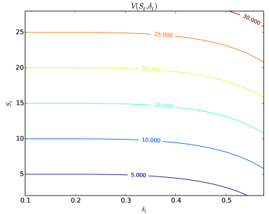
We observe from (3.14) that the shipping certificate value is separable in terms of the terminal spot price $S_{T}$ and market storage rate $\delta_{T}$ at time $T$. As we can see in Figure 2, the shipping certificate price $V(S_{T},\delta_{T})$ is increasing in both $S_{T}$ and $\delta_{T}$, and always dominates $S_{T}.$ When the market storage rate $\delta_{T}$ is below the critical level $\delta^{*}$ at time $T$, the shipping certificate price is equal to the spot price $S_{T}$, implying an immediate exercise by the holder. In this model, the non-convergence or basis is determined by the market storage rate $\delta_{T}$ since the exercise and liquidation strategies do not depend on $S_{T}$ at all.

In fact, the basis is roughly proportional to both the present value of the storage differential $\delta_{T}-\widehat{\delta}$ and the present value of the the average storage differential $\nu-\widehat{\delta}$. If $\delta_{t}<\widehat{\delta},$ then the value of the certificate decreases because it is currently cheaper to store at the real rate vs the certificate rate. Furthermore, if $\nu<\widehat{\delta},$ then the average storage rate is lower than the certificate rate, so the value of the shipping certificate decreases. This model explicitly states that agent must consider both the long-run storage differential $\nu-\widehat{\delta}$ and the immediate storage differential $\delta_{T}-\widehat{\delta}$ in choosing his exercise strategy $\delta^{*}.$ In particular, when we set the parameters $\zeta=0,$ $\kappa=0$ and $\nu=\delta,$ the problem reduces to the case with a constant market storage rate. In this case, the optimal exercise level becomes $\delta^{*}=\widehat{\delta}-c_{1}r,$ and the basis is completely linearly proportional to the storage differential $\delta-\widehat{\delta}$. After exercising the shipping certificate and thus receiving the grain, there is no benefit to sell the grain early ($\eta^{*}=\infty$). This is due to the martingale property of the spot price.

According to Proposition 1, the critical level $\delta^{*}$ determines the time $\tau^{*}$ to exercise the shipping certificate, and thus, plays a role in the non-convergence of the futures at maturity. Indeed, the higher the critical level $\delta^{*},$ the more likely the agent will exercise the shipping certificate at maturity, resulting in zero non-convergence. In contrast, a low $\delta^{*}$ implies a high likelihood of non-convergence at maturity. In fact, when $c_{1}=0$, the basis $w(S_{T},\delta_{T})>0$ if and only if $\delta_{T}>\delta^{*}$.

Furthermore, the conditional probability that a $T$-futures contract expires with a strictly positive basis is given by

$$\mathbb{Q}(w(S_{T},\delta_{T})>0|\mathcal{F}_{t})=1-\Phi\left(z_{t,T}^{*}\right),$$ (3.18)

where

$$\begin{split}z_{t,T}^{*}&=\frac{\delta^{*}-\bar{\nu}_{t,T}}{\bar{\zeta}_{t,T}}\,,\\ \bar{\nu}_{t,T}&=\delta_{t}e^{-\kappa(T-t)}+\nu(1-e^{-\kappa(T-t)})\,,\\ \bar{\zeta}_{t,T}^{2}&=\frac{\zeta^{2}}{2\kappa}\left(1-e^{-2\kappa(T-t)}\right)\,,\end{split}$$ (3.19)

and $\Phi$ is the standard normal cdf. In particular, the probability of a strictly positive basis depends solely on the current storage rate $\delta_{t}$ and the long run parameters of $(\delta_{t})_{t\geq 0}.$ This probability is completely independent of the realization $S_{t}$ at any time $t$, or its driving parameters $r$ and $\sigma!$ Furthermore, since non-convergence at maturity is undesirable behavior, we would like to know precisely how the parameters of our model affect $\delta^{*}$. Differentiating (3.15) with respect to $\widehat{\delta}$, $c_{1}$, and $\nu$, respectively, we obtain the sensitivity in each of these parameters.

$$\frac{d\delta^{*}}{d\widehat{\delta}}=h(\delta^{*})\left(1+\frac{\kappa}{r}\right)\geq 0,\quad\frac{d\delta^{*}}{d\nu}=-h(\delta^{*})\frac{\kappa}{r}\leq 0,\quad\frac{d\delta^{*}}{dc_{1}}=-h(\delta^{*})\left(\kappa+r\right)\leq 0,$$ (3.20)

where we have defined

$$h(\delta^{*}):=\frac{H^{\prime}(\delta^{*})^{2}}{H(\delta^{*})H^{\prime\prime}(\delta^{*})}\geq 0.$$

The function $h$ is positive because $H$ is positive, increasing, and convex. Therefore, we deduce the properties of the optimal exercise threshold $\delta^{*}$.

Corollary 1.

Under the Martingale Model defined in (3.1) and (3.2), the optimal stopping threshold $\delta^{*}$ is increasing with respect to $\widehat{\delta},$ but decreasing with respect to $\nu$ and $c_{1}.$

Having solved the certificate pricing problem, we proceed to examine how the storage optionality propagates to futures prices. At time $T$, the agent will exercise if storage rate $\delta_{T}$ is lower than the critical level $\delta^{*}$. Therefore, a higher $\delta^{*}$ increases the chance an agent will exercise the shipping certificate immediately upon the futures expiration. A higher certificate storage rate $\widehat{\delta}$ increases $\delta^{*}$ and hence lowers the probability of non-convergence. On the other hand, a higher average storage rate $\nu$ increases the probability of non-convergence. This occurs due to the incentive to store in the cheaper market: if the certificate storage rate is higher (resp. lower) than the market rate, then the agent will exercise sooner (resp. lower).

When calculating the derivatives in (3.20), the magnitude of each derivative is roughly proportional to $\kappa$, the rate of mean reversion of the storage rate $\delta_{t}$. Indeed, as $\kappa$ increases, the long run effect of $\nu$ dominates, acting as an amplifier on $\delta^{*}.$ Therefore, under higher $\kappa,$ if the storage differential $\nu-\widehat{\delta}$ is positive, the basis increases more, whereas if $\nu-\widehat{\delta}$ is negative, the basis increases less. Intuitively, since the value $c_{1}$ increases the agent’s cost to exercise, it is expected, as seen in (3.20), that $\delta^{*}$ is decreasing in $c_{1}$. Lastly, after exercising, the agent’s liquidation timing $\eta^{*}$ is trivial, so the liquidation cost $c_{2}$ does not affect the exercise level $\delta^{*}$.

Next, we compute the futures price using the shipping certificate price given in Proposition 1. It follows from the property of the OU process that $\delta_{T}|\delta_{t}$ is normally distributed with parameters $\bar{\nu}_{t,T}$ and $\bar{\zeta}_{t,T}$ which are given in (3.19). Following the definition in (3.6), the futures price is given by

$$\begin{split}F(t,S_{t},\delta_{t};T)=&\quad\mathbb{E}\left[S_{T}|\mathcal{F}_{t}\right]+\frac{1}{\kappa+r}\mathbb{E}\left[\left(\delta_{T}-\frac{H(\delta_{T})}{H(\delta^{*})}-\widehat{\delta}+\frac{\kappa(\nu-\widehat{\delta})}{r}\right)\mathbf{1}\{\delta_{T}\geq\delta^{*}\}|\mathcal{F}_{t}\right]\\ &-c_{1}\mathbb{Q}(\delta_{T}<\delta^{*}|\mathcal{F}_{t})\,.\end{split}$$

By computing the conditional truncated expectations of $S_{T}$ and $\delta_{T}$, we obtain an explicit formula for the futures price.

Corollary 2.

Under the Martingale Model defined in (3.1) and (3.2), the grain futures price is given by

$$F(t,S_{t},\delta_{t};T)= \quad e^{r(T-t)}\left[S_{t}+\frac{\nu}{r}\left(1-e^{-r(T-t)}\right)+\frac{\delta_{t}-\nu}{\kappa+r}\left(1-e^{-(\kappa+r)(T-t)}\right)\right]$$ (3.21)

$$\quad+\frac{1}{\kappa+r}\left[\bar{\nu}_{t,T}+\frac{\phi\left(z_{t,T}^{*}\right)}{1-\Phi\left(z_{t,T}^{*}\right)}\bar{\zeta}_{t,T}-\int_{z_{t,T}^{*}}^{\infty}\frac{H(\bar{\nu}_{t,T}+\bar{\zeta}_{t,T}u)}{H^{\prime}(\delta^{*})}\phi(u)du\right.$$ (3.22)

$$\quad+\left.\left(\frac{\kappa(\nu-\widehat{\delta})}{r}-\widehat{\delta}\right)\left(1-\Phi\left(z_{t,T}^{*}\right)\right)\right]-c_{1}\Phi\left(z_{t,T}^{*}\right),\qquad t\leq T,$$ (3.23)

where $z_{t,T}^{*},$ $\bar{\nu}_{t,T}$ and $\bar{\zeta}_{t,T}$ are given in (3.19), and $\phi$ and $\Phi$ are the standard normal pdf and cdf respectively.

We note that like the shipping certificate prices, futures prices can be separated into an expectation that depends on $S_{t}$ and another involving $\delta_{t}$. Despite the separation, since $\delta_{t}$ appears in the diffusion for $S_{t}$, the two stochastic factors are not independent. The futures price encapsulates a number of components: (i) the risk-neutral expectation of the future spot price; (ii) expected future basis $w(S_{T},\delta_{T})$ (see (3.5)); and (iii) expected future exercise cost $c_{2}.$ Thus, by accounting for the expected future basis resulting from the storage differential $\delta_{t}-\widehat{\delta},$ the futures price for all $t\leq T$ in a market with shipping certificates carries a premium over the price of a futures contract that delivers just the grain at time $T$. We therefore demonstrate that anticipated future storage differentials can impact current futures prices, including the contracts that are far from expiry.

With an understanding on the theoretical behavior of grain futures prices under the Martingale Model, we now calibrate to empirical data, and discuss the results and economic implications. We obtain futures prices from 2004-2011 for CBOT corn, wheat and soybeans contracts using Bloomberg terminal. We obtain spot prices from 2004-2011 for CBOT corn, wheat, and soybeans from an average of daily sale prices of several Illinois grain depots. We also obtain the empirical certificate storage rate $\widehat{\delta}$, quoted in $\$/bushel,$ from the CBOT website. For the interest rate in our model, we use the 3-month LIBOR rate observed on the same date. There are several quoted prices for spot grain, differing only in the quality of the grain. This quality option allows the short to choose the grade he wishes to deliver, subject to some prior fixed conversion multiplier of the settlement price. In order to obtain a single series of spot prices, for every time $t$ we use the then cheapest-to-deliver price as the spot price for grain.

Recall that the basis $w(S_{T},\delta_{T})$ is the premium of the certificate price $V(T,S_{T})$ over the spot price $S_{T}.$ at time $T$. On the day $t=0,$ we have the empirical futures prices $(F_{k})_{k=0}^{N}$ with maturities $(T_{k})_{k=0}^{N},$ and a known spot price $F_{0}=S_{0};$ we seek a model-consistent futures curve $\textbf{F}_{k}(\nu,\kappa,\zeta,\delta_{0})$ for $k=0,1,\ldots,N$ which best fits the empirical futures prices, given model parameters $(\nu,\kappa,\zeta)$ and $\delta_{0}$, with the model futures prices given in (3.23). Under this setup, the best fit calibrated futures curve $\textbf{F}_{k}^{*}$ for $k=0,1,\ldots,N$ minimizes the sum of squared errors (SSE) between the empirical futures curve and the model futures curve. Furthermore, the best-fit parameters are defined to be $(\nu^{*},\kappa^{*},\zeta^{*},\delta_{0}^{*})$ the model parameters which achieve the best fit futures curve. The other exogenous parameters $(r,S_{t},\widehat{\delta},c_{1},c_{2})$ are directly determined via contract specifications. Precisely, the calibrated parameters and the resulting futures curve are found from

$$\begin{split}(\nu^{*},\kappa^{*},\zeta^{*},\delta_{0}^{*})&=\operatorname*{arg\,min}_{\nu,\kappa,\zeta,\delta_{0}}\sum_{k=0}^{N}(F_{k}-\textbf{F}_{k}(\nu,\kappa,\zeta,\delta_{0}))^{2}\\ \textbf{F}_{k}^{*}&=\vec{\textbf{F}}(\nu^{*},\kappa^{*},\zeta^{*},\delta_{0}^{*})\qquad k=0,1,\ldots N.\end{split}$$ (3.24)

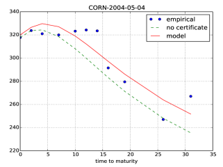
In Figure 3, we calibrate the Martingale Model to the corn futures prices on two dates selected to show two characteristically different futures curves. On the left panel, the futures curve is downward sloping. With the expiring futures price and spot price being $3.17 and $2.81, respectively, a positive basis is observed. Intuitively, given that the current market storage rate is higher than the certificate rate ($\delta_{0}^{*}>\widehat{\delta}$), the agent thus prefers the certificate storage rate over the market rate and will wait to exercise the certificate, resulting in a positive basis. The current storage rate $\delta_{0}^{*}$ is also higher than the estimated long-run storage rate $\nu^{*}$. Therefore, the model suggests that in the long run, a convenience yield will dominate, leading to a downward sloping futures curve. In contrast, the right panel also reflects a positive basis, but the futures curve is upward sloping.

Figure 4 displays the calibrated futures curves under the Martingale Model for wheat on two dates when the futures market is in backwardation and contango, respectively. Again, non-convergence is observed on each of these two dates as the expiring futures price dominates the spot price. On the left panel, the futures curve is upward sloping while the right panel shows that the futures curve is downward sloping. In this case, the current market storage rate satisfies $\delta_{0}^{*}>\widehat{\delta}$, so it is optimal for the agent to continue to store at the lower certificate storage rate. Hence, the value of the associated timing option to exercise the shipping certificate yields a positive basis.

In addition, we consider the differences between the model futures curve and the futures curve generated without considering the timing options. To be precise, let the ‘no certificate’ futures price $\psi(t,S_{t},\delta_{t};T)$ be

$$\begin{split}\psi(t,S_{t},\delta_{t};T)&=\mathbb{E}[S_{T}|\mathcal{F}_{t}],\\ &=e^{r(T-t)}\left[S_{t}+\frac{\nu}{r}\left(1-e^{-r(T-t)}\right)+\frac{\delta_{t}-\nu}{\kappa+r}\left(1-e^{-(\kappa+r)(T-t)}\right)\right].\end{split}$$ (3.25)

This follows from direct calculations and resembles the first line of (3.23). In Figure 3, we plot the values of $\psi(0,S_{0},\delta_{0}^{*};T_{i})$ for $i=0\dots N,$ using the same fitted parameters from our model $(\nu^{*},\kappa^{*},\zeta^{*},\delta_{0}^{*})$ and the constraint that $S_{t}=F_{0},$ the empirical terminal futures price. In other words, we ignore the data on spot grain prices, so there is initially zero basis, as would be the case under physical delivery, as opposed to receiving the shipping certificate upon expiration. As expected, the model futures prices with shipping certificate dominate the those without one, for all maturities. As seen in Figure 3, the premium of the shipping certificate over the spot as the delivery item tends to be higher for longer maturities. Finally, the Martingale Model fits both backwardated and upward-sloping futures curves well.

Figure 3: Calibrating the Martingale Model to empirical corn futures prices. The $x$-axis is time to maturity in months and the $y$-axis is the price of a bushel of corn in $cents.$ The ‘no certificate’ curve is taken from equation (3.25). We use the fitted parameters from the ‘model’ curve as inputs for the ‘no certificate’ curve to illustrate the premium. Fitted parameters: (left) $\nu^{*}=-0.48,$ $\kappa^{*}=0.0015,$ $\zeta^{*}=0.0161,$ and $\delta_{0}^{*}=1.2532$; (right) $\nu^{*}=0.832,$ $\kappa^{*}=0.021,$ $\zeta^{*}=0.428,$ and $\delta_{0}^{*}=0.782.$ Other parameters are $r=0.017,$ $S_{0}=\{282,167\}$ (cents), $\widehat{\delta}=0.55$, and $c_{1},c_{2}=0.$

Figure 4: Calibrating the Martingale Model to empirical wheat futures prices. The $x$-axis is time to maturity in months and the $y$-axis is the price of a bushel of wheat in $cents.$ The ‘no certificate’ curve is taken from equation (3.25). Fitted parameters: (left) $\nu^{*}=0.91,$ $\kappa^{*}=0.035,$ $\zeta^{*}=0.14,$ and $\delta_{0}^{*}=0.871$; (right) $\nu^{*}=-0.22,$ $\kappa^{*}=0.0032,$ $\zeta^{*}=0.61,$ and $\delta_{0}^{*}=1.44.$ We use the fitted parameters from the ‘model’ curve as inputs for the ‘no certificate’ curve to illustrate the premium. Other parameters are $r=0.017,$ $S_{0}=\{273,772\}$ (cents), $\widehat{\delta}=0.55$, and $c_{1},c_{2}=0.$

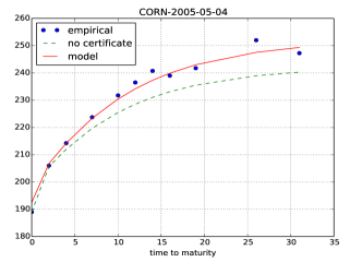
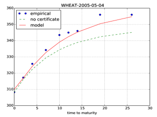
Our model postulates that the non-convergence occurs when the market storage rate is significantly higher than the certificate storage rate. Therefore, if the two rates are brought into alignment, we expect that the basis to diminish. Indeed, after years of high basis, the two exchanges, CBOT and KCBOT, enacted a series of reforms on the wheat futures to address the non-convergence phenomenon. During February 2009 to May 2011, both exchanges instituted a one-time hike in the formerly constant storage rates, and subsequently adopted a variable certificate storage rate for all wheat contracts, thus better aligning the certificate and market storage rates. For corn and soybeans, the exchanges merely raised the constant certificate storage rates once in Jan 2011. According to (3.18), these policy changes would decrease the likelihood of non-convergence. In Table 1, we compare the average basis before and after the policy implementation for each commodity. The average basis decreased by 6.57% for corn, 3.42% for soybeans, and 2.29% for wheat, suggesting that the effectiveness of changing the certificate storage rate. In fact, the study by Aulerich and Hoffman (2013) finds that introducing a variable certificate storage rate can significantly reduce non-convergence.

Commodity	Average Basis (pre)	Max Basis (pre)	Average Basis (post)	Max Basis (post)
Corn	9.11%	27.52%	2.54%	13.50%
Soybeans	4.31%	12.96%	0.89%	5.61%
Wheat	1.32%	14.10%	-0.97%	7.05%

Table 1: Basis summary during 2004-2014 before (pre) and after (post) CBOT introduced new certificate policies to facilitate convergence in the corn, soybeans, and wheat futures markets. For corn and soybeans futures, the policy changed in in January 2011. For wheat contracts, a variable storage rate policy was introduced in July 2010. For comparison across commodities, the basis here is computed in percentage at expiration according to [(futures price/spot price)-1]$\times$100%.

4 Local Stochastic Storage Model

We now consider an alternative to the Martingale Model. Since the commodity cannot necessarily be continuously traded, the market is incomplete, and one can specify a non-martingale evolution for the commodity price under the no-arbitrage risk-neutral measure. Commodities have the unique property that production can be increased or decreased in response to high or low prices, respectively. In addition, commodities can be consumed through production of end-goods (for example, turning corn into ethanol). In times of scarcity, production will increase to lower prices; in times of surplus, production will decrease while consumption continues to increase prices. Thus, the production and consumption process unique to commodities imply a mean-reverting price structure as suggested by Deaton and Laroque (1996).

Hence, we propose an exponential OU (XOU) model for the spot price. Under the risk-neutral measure $\mathbb{Q}$, the log-spot price of the grain, denoted by $U_{t}=\log S_{t}$, follows the OU process

$$dU_{t}=\alpha(\mu-U_{t})dt+\sigma dW_{t},$$ (4.1)

where $W$ is standard Brownian motion under $\mathbb{Q},$ $\mu$ is the long-run mean, $\alpha$ is the rate of mean reversion, and $\sigma$ is the volatility of the log-spot price. We impose the further regularity condition that $\sigma<\sqrt{2\alpha}.$

The market rate of storage $\delta_{t}$ is locally determined by the spot price through

$$\delta_{t}=\beta U_{t}+\gamma.$$ (4.2)

We typically set the coefficient $\beta\geq 0$ so that the storage cost increases linearly with the log-price of the commodity, with a possibly flat storage rate $\gamma>0$. In summary, we have described a local stochastic storage approach, whereby the market storage rate in (4.2) is a function of the stochastic spot price that follows the exponential OU model in (4.1). Henceforth, we shall refer it as the XOU Model.

Denote by $\mathbb{G}\equiv(\mathcal{G}_{t})_{t\geq 0}$ the filtration generated by the log-spot price $(U_{t})_{t\geq 0}$. Also, let $\mathcal{S}$ be the set of all $\mathbb{G}$-stopping times, and $\mathcal{S}_{s,u}$ the set of $\mathbb{G}$-stopping times bounded by $[s,u]$. Note that $\delta_{t}$ is a function of $U_{t}$, the optimal liquidation problem is given by

$$J(U_{t})=\sup_{\eta\in\mathcal{S}_{t,\infty}}\mathbb{E}\left[e^{-r(\eta-t)}\left(\exp(U_{\eta})-c_{2}\right)-\int_{t}^{\eta}\delta_{u}e^{-r(u-t)}du|\mathcal{G}_{t}\right],$$ (4.3)

which applies after the shipping certificate is exercised at time $\tau$. The optimal timing problem to exercise the shipping certificate is given by

$$V(U_{T})=\sup_{\tau\in\mathcal{S}_{T,\infty}}\mathbb{E}\left[e^{-r(\tau-T)}\left(J(U_{\tau})-c_{1}\right)-\int_{T}^{\tau}\widehat{\delta}e^{-r(u-T)}du|\mathcal{G}_{T}\right].$$ (4.4)

Since the shipping certificate serves as the delivery item instead of the actual grain, the futures price $F(t,U_{t};T)$ at $t$ for the contract expiring at $T$ is given by

$$F(t,U_{t};T)=\mathbb{E}[V(U_{T})|\mathcal{G}_{t}].$$ (4.5)

We now denote the operator from (3.8) by $\mathcal{L}\equiv\mathcal{L}^{\alpha,\mu,\sigma}$, which is the infinitesimal generator for the OU process $U$. To solve for the certificate price and the agent’s optimal policy, we solve the ODE

$$\mathcal{L}f(u)-rf(u)=0,$$ (4.6)

which has the general solutions, $H(u;\alpha,\mu,\sigma)$ and $G(u;\alpha,\mu,\sigma),$ where $\mathcal{L},$ $H,$ and $G$ are defined in (3.8), (3.10) and (3.11). In this section, without ambiguity, we denote $H(u)\equiv H(u;\alpha,\mu,\sigma)$ and $G(u)\equiv G(u;\alpha,\mu,\sigma)$, both of which will play a role in the solution for $J$ and $V.$

Proposition 2.

Under the XOU Model defined in (4.1) and (4.2):

1. The liquidation value is given by

   $$J(u)=\begin{cases}AH(u)-\frac{1}{\alpha+r}\left[\beta u+\gamma+\frac{\alpha(\beta\mu+\gamma)}{r}\right]&\text{ if $u<u^{*}$,}\\ e^{u}-c_{2}&\text{ if }u\geq u^{*}.\end{cases}$$ (4.7)

2. The certificate price is given by

   $$V(u)=\begin{cases}e^{u}-c_{1}-c_{2}&\text{ if }u>\overline{u}^{**},\\ BH(u)+CG(u)-\frac{\widehat{\delta}}{r}&\text{ if }\underline{u}^{**}\leq u\leq\overline{u}^{**},\\ AH(u)-\frac{1}{\alpha+r}\left[\beta u+\gamma+\frac{\alpha(\beta\mu+\gamma)}{r}\right]-c_{1}&\text{ if }u<\underline{u}^{**},\end{cases}$$ (4.8)

   where

   $$\begin{split}A&=\frac{e^{u^{*}}+\frac{\beta}{\alpha+r}}{H^{\prime}(u^{*})}\,,\\ B&=\frac{e^{\overline{u}^{**}}G^{\prime}(\underline{u}^{**})-\left(AH^{\prime}(\underline{u}^{**})-\frac{\beta}{\alpha+r}\right)G^{\prime}(\overline{u}^{**})}{H^{\prime}(\overline{u}^{**})G^{\prime}(\underline{u}^{**})-H^{\prime}(\underline{u}^{**})G^{\prime}(\overline{u}^{**})}\,,\\ C&=\frac{e^{\overline{u}^{**}}H^{\prime}(\underline{u}^{**})-\left(AH^{\prime}(\underline{u}^{**})-\frac{\beta}{\alpha+r}\right)H^{\prime}(\overline{u}^{**})}{H^{\prime}(\underline{u}^{**})G^{\prime}(\overline{u}^{**})-H^{\prime}(\overline{u}^{**})G^{\prime}(\underline{u}^{**})}\,,\end{split}$$ (4.9)

   and the optimal thresholds $u^{*}$, $\overline{u}^{**}$ and $\underline{u}^{**}$ satisfy the equations:

   $$\begin{split}AH(u^{*})-\frac{1}{\alpha+r}\left[\beta u^{*}+\gamma+\frac{\alpha(\beta\mu+\gamma)}{r}\right]&=e^{u^{*}}-c_{2}\,,\\ BH(\overline{u}^{**})+CG(\overline{u}^{**})-\frac{\widehat{\delta}}{r}&=e^{\overline{u}^{**}}-c_{1}-c_{2}\,,\\ BH(\underline{u}^{**})+CG(\underline{u}^{**})-\frac{\widehat{\delta}}{r}&=AH(\underline{u}^{**})-\frac{1}{\alpha+r}\left[\beta\underline{u}^{**}+\gamma+\frac{\alpha(\beta\mu+\gamma)}{r}\right]-c_{1}.\end{split}$$ (4.10)

   The optimal exercise and liquidation times, respectively, are given by

   $$\begin{split}\tau^{*}&=\inf\{\,t\geq T:U_{t}\leq\underline{u}^{**}\,\text{ or }\,U_{t}\geq\overline{u}^{**}\,\}\,,\\ \eta^{*}&=\inf\{\,t\geq\tau^{*}:U_{t}\geq u^{*}\,\}\,.\\ \end{split}$$ (4.11)

The liquidation value $J(u)$ is entirely determined by the critical level $u^{*}$ at which the agent will sell the physical grain. When the log-spot price $U_{t}$ surpasses $u^{*}$, both the storage cost $\delta_{t}$ and spot price $S_{t}$ will be high. Since the asset price is mean-reverting, intuitively there is a potential advantage to early liquidation before the asset reverts back to a lower value. In the holding region $\{u<u^{*}\}$ corresponding to low spot prices, the agent pays the present value of the storage rate $\beta u+\gamma,$ and the present value of the average storage rate $\beta\mu+\gamma.$ The conflict between increasing spot prices and higher storage rates, both of which are driven by $U_{t},$ determines when the agent liquidates. Thus, both instantaneous storage rates and the long-run storage rates affect the certificate price.

On the other hand, the certificate value $V(u)$ is determined by $two$ stopping levels: the optimal exercise threshold $\underline{u}^{**}$ and the optimal liquidation threshold $\overline{u}^{**}.$ When the spot price surpasses $\overline{u}^{**}$, the agent exercises $and$ liquidates to take advantage of temporarily higher spot prices, while avoiding higher storage rates. On the other hand, when the spot price decreases below $\underline{u}^{**},$ the agent exercises but does $not$ liquidate, because he wants to take advantage of a temporarily lower storage rate, storing in the real market at rate $\delta_{t}$ instead of at the certificate rate $\widehat{\delta}.$ Recall that due to our specification of the optimal stopping times $\eta^{*}$ and $\tau^{*},$ the stopping levels satisfy $\overline{u}^{**}\geq u^{*}\geq\underline{u}^{**}.$

Figure 5: Optimal stopping levels for $[\underline{u}^{**},u^{*},\overline{u}^{**}]$, with default parameters $r=0.03,$ $U_{t}=\log 5,$ $\gamma=0,$ $\widehat{\delta}=0.2,$ $\beta=0.08,$ $c_{1}=0,$ $c_{2}=0,$ $\mu=\log{30}$, $\alpha=0.1$, $\sigma=0.2$. We vary the parameters $\beta$ and $\hat{\delta}$ respectively in these plots.

Figure 6: Immediate value $\exp(u)-c_{1}-c_{2},$ liquidation value $J(u),$ and certificate price $V(u)$. The optimal stopping levels are given by $\underline{u}^{**}=0.337,$ $u^{*}=3.485,$ $\overline{u}^{**}=3.534.$ Parameters are $r=0.03,$ $\gamma=0,$ $\widehat{\delta}=0.17,$ $\beta=0.10,$ $c_{1}=0,$ $c_{2}=0,$ $\mu=\log{30}$, $\alpha=0.1$, $\sigma=0.2$.

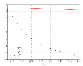
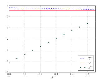
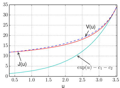
Figure 5 further illustrates the dependence of the three stopping levels $[\underline{u}^{**},u^{*},\overline{u}^{**}]$ on the parameters $\beta$ and $\widehat{\delta}.$ As $\beta$ increases, the gap between $\underline{u}^{**}$ and $\overline{u}^{**}$ increases, so does the basis. However, as $\beta\to 0,$ the market storage rate goes to 0 in this example, inducing the agent to exercise as soon as the futures expires and store in the real market. Consequently, the region $\{\underline{u}^{**},\overline{u}^{**}\}$ for holding the certificate vanishes, which also means that all three thresholds, $\underline{u}^{**},u^{*}$, and $\overline{u}^{**}$ converge to the same value representing the optimal level to liquidate the grain. A similar pattern is observed when the certificate storage rate $\widehat{\delta}$ increases since the agent will again be incentivized to exercise the shipping certificate immediately to store in the real market.

Figure 6 also reflects the relationship among the certificate price, liquidation value, and payoff from immediate exercise and liquidation. Note that

$$V(u)\geq J(u)\geq\exp(u)-c_{1}-c_{2},$$

i.e. the shipping certificate price dominates the liquidation value, which convexly dominates the immediate exercise value. The liquidation value is significantly higher than the immediate exercise value, especially as $u\to-\infty.$ The value of $J(u)$ does not decrease as much as the immediate exercise value. Because the asset is mean reverting and the optionality is perpetual, the asset value is almost guaranteed to be eventually profitable. In this model, the ability to choose between two rates of storage adds merely a modest basis to the liquidation value. With the parameters in Figure 5, the maximum percent difference between $V(u)$ and $J(u)$ is 12.57%.

Recall that the basis $w(U_{t})$ is defined as the difference between certificate and spot prices at maturity. As we established from a model-free argument, the basis $w(U_{t})\geq 0.$ Therefore, a positive basis occurs when the agent chooses a strategy which is different than exercising and liquidating ($\eta^{*}>\tau>T$). In this scenario, the agent either waits to exercise because storage rates are too high to exercise and spot prices are too low to liquidate, or he has exercised to take advantage of lower storage prices but the spot price is too low to liquidate. In our model the probability of non-convergence depends completely on $\overline{u}^{**}.$ In particular, if $c_{1}=0$ and $c_{2}=0,$ then the basis $w(U_{T})>0$ iff $U_{T}<\overline{u}^{**}.$ Thus, the probability that there is a strictly positive basis at time $t$ for a contract maturing at $T\geq t$ is

$$\mathbb{Q}\left(w(U_{T})>0\,|\,\mathcal{G}_{t}\right)=\Phi\left(\frac{\overline{u}^{**}-\bar{\mu}_{t,T}}{\bar{\sigma}_{t,T}}\right),$$ (4.12)

where

$$\begin{split}\bar{\mu}_{t,T}&=U_{t}e^{-\alpha(T-t)}+\mu(1-e^{-\alpha(T-t)}),\\ \bar{\sigma}_{t,T}^{2}&=\frac{\sigma^{2}}{2\alpha}(1-e^{-2\alpha(T-t)}).\end{split}$$ (4.13)

Finally, in order to calibrate our model for empirical analysis, we derive futures prices by taking an expectation of the certificate prices.

Under the OU model, the conditional log spot price $U_{T}|U_{t}$ is normally distributed with parameters $\bar{\mu}_{t,T}$ and $\bar{\sigma}_{t,T}$ given in (4.13). The result then follows from computing the associated conditional truncated expectations:

$$\begin{split}&F(t,U_{t};T)=\quad\mathbb{E}\left[\left(e^{U_{T}}-c_{1}-c_{2}\right)\mathbf{1}\{U_{T}>\overline{u}^{**}\}|U_{t}\right]\\ &\qquad\qquad+\mathbb{E}\left[\left(BH(U_{T})+CG(U_{T})-\frac{\widehat{\delta}}{r}\right)\mathbf{1}\{\underline{u}^{**}\leq U_{T}\leq\overline{u}^{**}\}|U_{t}\right]\\ &\qquad\qquad+\mathbb{E}\left[\left(AH(u)-\frac{1}{\alpha+r}\left[\beta U_{T}+\gamma+\frac{\alpha(\beta\mu+\gamma)}{r}\right]-c_{1}\right)\mathbf{1}\{U_{T}<\underline{u}^{**}\}|U_{t}\right]\end{split}$$ (4.14)

Corollary 3.

The futures price $F(t,U_{t};T)$ under the XOU Model defined in (4.1) and (4.2) is given by

$$F(t,U_{t};T) =\quad\exp\left(\bar{\mu}_{t,T}+\frac{\bar{\sigma}_{t,T}^{2}}{2}\right)\frac{\Phi\left(\bar{\sigma}_{t,T}-\overline{z}_{t,T}^{**}\right)}{1-\Phi\left(\overline{z}_{t,T}^{**}\right)}-(c_{1}+c_{2})\left(1-\Phi\left(\overline{z}_{t,T}^{**}\right)\right)$$ (4.15)

$$\quad+\int_{\underline{z}_{t,T}^{**}}^{\overline{z}_{t,T}^{**}}(BH(\bar{\mu}_{t,T}+\bar{\sigma}_{t,T}v)+CG(\bar{\mu}_{t,T}+\bar{\sigma}_{t,T}v))\phi(v)dv$$ (4.16)

$$\quad-\frac{\widehat{\delta}}{r}\left(\Phi\left(\overline{z}_{t,T}^{**}\right)-\Phi\left(\underline{z}_{t,T}^{**}\right)\right)+\int_{-\infty}^{\underline{z}_{t,T}^{**}}AH(\bar{\mu}_{t,T}+\bar{\sigma}_{t,T}v)dv$$ (4.17)

$$\quad-\frac{\beta}{\alpha+r}\left(\bar{\mu}_{t,T}-\frac{\phi\left(\underline{z}_{t,T}^{**}\right)}{\Phi\left(\underline{z}_{t,T}^{**}\right)}\bar{\sigma}_{t,T}\right)-\left(\frac{\gamma}{\alpha+r}+\frac{\alpha(\beta\mu+\gamma)}{r(\alpha+r)}+c_{1}\right)\Phi\left(\underline{z}_{t,T}^{**}\right),$$ (4.18)

where

$$\overline{z}_{t,T}^{**}=\frac{\overline{u}^{**}-\bar{\mu}_{t,T}}{\bar{\sigma}_{t,T}},\qquad\underline{z}_{t,T}^{**}=\frac{\underline{u}^{**}-\bar{\mu}_{t,T}}{\bar{\sigma}_{t,T}},$$ (4.19)

and $\bar{\mu}_{t,T},$ and $\bar{\sigma}_{t,T}$ are defined in (4.13).

We calibrate our model futures curve to empirical corn, wheat and soybeans data and consider the accuracy and economic implications. Refer to Table 1 for details of each contract’s specification. Consider the futures curve at time $t=0.$ Recall that the best-fit futures curve can be defined in the following manner. Let the futures prices at time $T_{k}$ be $F_{k},$ for maturity times $(T_{k})_{k=0}^{N},$ with $F_{0}=\exp(U_{0})=S_{0},$ so the futures price at $T_{0}=0$ is just the market quoted settlement price. Denote the model futures curve generated at time $T_{k}$ by the parameters $(\beta,\gamma,\mu,\alpha,\sigma)$ be denoted $\textbf{F}_{k}(\beta,\gamma,\mu,\alpha,\sigma).$

The best fit futures curve $\textbf{F}_{k}^{*}$ for $k=0,1,\ldots,N$ minimizes the weighted sum of squared errors (SSE) between the empirical futures curve and the model futures curve at time $t.$ Furthermore, the best-fit parameter is defined to be $(\beta^{*},\gamma^{*},\mu^{*},\alpha^{*},\sigma^{*})$ the model parameters which achieve the best fit futures curve. The other exogenous parameters $(r,U_{t},\widehat{\delta},c_{1},c_{2})$ are directly determined via contract specifications (see Table 1).

$$\begin{split}(\beta^{*},\gamma^{*},\mu^{*},\alpha^{*},\sigma^{*})&=\operatorname*{arg\,min}_{\beta,\gamma,\mu,\alpha,\sigma}\sum_{k=0}^{N}(F_{k}-\textbf{F}_{k}(\beta,\gamma,\mu,\alpha,\sigma))^{2}\\ \textbf{F}_{k}^{*}&=\textbf{F}_{k}(\beta^{*},\gamma^{*},\mu^{*},\alpha^{*},\sigma^{*})\qquad k=0,1,\ldots,N.\end{split}$$ (4.20)

The $corn$ futures curves calibrated from the XOU Model are illustrated in Figure 7. We have selected the two dates to illustrate two characteristically different futures curves. On the left panel, the futures curve that is upward sloping. With the expiring futures price and spot price being 317 and 281 (cents), respectively, a positive basis is observed. The current storage rate $\delta_{0}^{*}=106.00,$ and the long run storage rate $\beta^{*}\mu^{*}+\gamma^{*}=89.55$ are both higher than the certificate rate $\widehat{\delta}.$ This storage rate spread leads to the positive basis, while the long run storage rate anticipates a future basis. Furthermore, the current spot price $U_{0}>\mu^{*},$ which indicates that the spot price will likely fall in the future, and results in a downward-sloping futures curve. On the right panel, the futures curve is upward sloping and the basis is more modest. The spot price current satisfies $U_{0}<\mu^{*},$ so the spot price is expected to rise in the future, generating a more contango futures curve.

In Figure 8, we see the results of our empirical calibration under the XOU model for $wheat$ on two dates. The left panel shows a basis of around 12%, and the futures curve is upward sloping. The current storage rate $\delta_{0}^{*}=67.21,$ and the long run storage rate $\beta^{*}\mu^{*}+\gamma^{*}=69.84$ are both higher than the certificate rate $\widehat{\delta}.$ Therefore, the current storage rate leads to a positive basis, while the long run storage rate anticipates a future basis. Furthermore, the current spot price $U_{0}<\mu^{*},$ which indicates that the spot price will likely rise in the future, and results in an upward-sloping futures curve. In Figure 8 (right), the basis is more modest at 5%, while the futures curve is downward sloping. The current storage rate $\delta_{0}^{*}=60.71,$ is higher than the certificate storage rate, but the long run storage rate $\beta^{*}\mu^{*}+\gamma^{*}=53.87$ is lower than the certificate rate $\widehat{\delta}.$ Therefore, the current storage rate generates a smaller positive basis, while the long run storage rate anticipates little to no basis on the futures curve. Furthermore, the current spot price is higher than the estimated long-run mean ($U_{0}>\mu^{*}$), and the backwardated futures curve reflects the anticipation that the spot price will decrease in the future. This is consistent with the model’s mean-reverting dynamics for the spot price.

In addition, we consider the differences between the model futures curve and the futures curve generated without considering the timing options. To be precise, let the ‘no certificate’ futures curve $\psi(t,U_{t},\delta_{t};T)$ be

$$\psi(t,U_{t};T) =\mathbb{E}[S_{T}|\mathcal{G}_{t}]$$ (4.21)

$$=\exp\bigg{(}e^{-\alpha(T-t)}U_{t}+\mu(1-e^{-\alpha(T-t)})+\frac{\sigma^{2}}{4\mu}(1-e^{-2\alpha(T-t)})\bigg{)},$$ (4.22)

which can be found in (Leung et al., 2016, Sect. 2.2). In Figure 8, we plot the futures curve, described by $\psi(0,U_{0};T_{i})$ for $i=0\dots N,$ using the same fitted parameters from our model $(\mu^{*},\alpha^{*},\sigma^{*})$ and the initial assumption that $\exp(U_{0})=F_{0},$ the empirical terminal futures price. In other words, for the no-certificate case, we take the expiring futures price to be the spot price, and ignore the entire spot grain market prices. The last assumption means there is initially zero basis, as would be the case when physical grain is the delivery item.

Figure 7: Calibrating the XOU Model to the empirical corn futures prices. The $x$-axis is time to maturity in months and the $y$-axis is the price of a bushel of corn in $cents.$ The ‘no certificate’ curve is taken from equation (4.22). We use the fitted parameters from the ‘model’ curve as inputs for the ‘no certificate’ curve to illustrate the premium. Fitted parameters: (left) $\beta^{*}=16.12,$ $\gamma^{*}=15.08$ $\mu^{*}=4.62,$ $\alpha^{*}=0.058,$ and $\sigma^{*}=0.40.$ Fitted parameters for the rightmost panel are $\beta^{*}=10.75,$ $\gamma^{*}=15.10,$ $\mu^{*}=5.52,$ $\alpha^{*}=0.10,$ and $\sigma^{*}=0.12.$ Other parameters are $r=0.017,$ and (in cents) $S_{0}=\exp(U_{0})=\{281,167\}$, $\delta_{0}^{*}=106$, $\widehat{\delta}=55$ and $c_{1},c_{2}=0.$

Figure 8: Calibrating XOU model with local storage to the empirical wheat futures curve. The $x$-axis is time to maturity in months and the $y$-axis is the price of a bushel of wheat in $cents.$ The ‘no certificate’ curve is taken from equation (4.22). We use the fitted parameters from the ‘model’ curve as inputs for the ‘no certificate’ curve to illustrate the premium. Fitted parameters: (left) $\beta^{*}=9.98,$ $\gamma^{*}=11.22$ $\mu^{*}=5.83,$ $\alpha^{*}=0.08,$ and $\sigma^{*}=0.14.$ Fitted parameters for the rightmost panel are $\beta^{*}=7.13,$ $\gamma=14.16,$ $\mu^{*}=5.90,$ $\alpha^{*}=0.38,$ and $\sigma^{*}=0.91.$ Other parameters are $r=0.017,$ $U_{t}=\{5.61,6.65\},$ $\widehat{\delta}=55$ and $c_{1},c_{2}=0.$

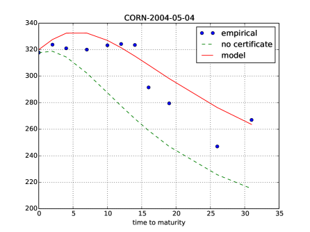
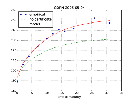
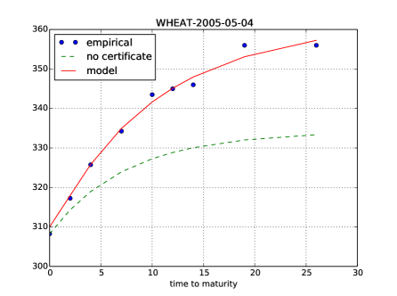
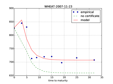
As shown earlier, the model prices of futures of all maturities with a shipping certificate dominate the respective contracts without one due to the timing options embedded in the shipping certificate. Furthermore, the difference increases as the futures maturity lengthens, indicating that the storage option exerts a more significant price impact over a longer period of time. In summary, we have shown that the timing options in a shipping certificate are a crucial component to explain the positive basis. As we have seen, the exponential OU model is able to capture forward anticipative behaviors of the basis and account for both backwardated and upwards-sloping futures curves.

Figure 9: Calibrating the Martingale Model (left) and the XOU Model (right) to the empirical soybeans futures curve. The $x$-axis is time to maturity in months and the $y$-axis is the price of a bushel of wheat in $cents.$ The ‘no certificate’ curve is taken from equations (3.25) and (4.22) respectively. The fitted parameters from the ‘model’ curve are used as inputs for the ‘no certificate’ curve to illustrate the premium. Fitted parameters: (left) $\nu^{*}=-0.44,$ $\kappa^{*}=0.023,$ $\zeta^{*}=0.92,$ and $\delta_{0}^{*}=1.42$; (right) $\beta^{*}=11.88,$ $\gamma^{*}=9.97$, $\mu^{*}=5.91,$ $\alpha^{*}=0.035,$ and $\sigma^{*}=0.95.$ Other parameters are $r=0.017,$ $S_{t}=1004.25,$ $\widehat{\delta}=55$ and $c_{1}=c_{2}=0.$

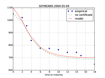
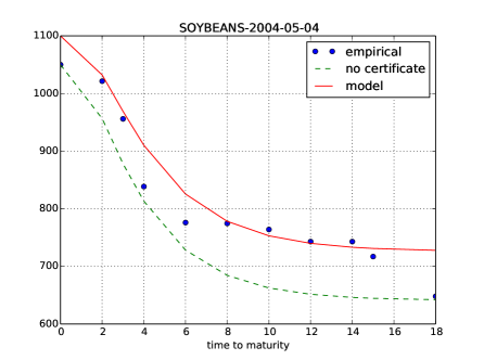
We close this section by comparing the empirical calibrations of the Martingale Model and the XOU Model in Figure 9. While both models are equally capable of estimating the immediate basis and fitting the empirical futures prices, the value of the timing option embedded in the shipping certificate is significantly higher under the XOU Model than the Martingale Model. This can be seen from the spread between the ‘model’ curve (shipping certificate delivery) and the ‘no certificate’ curve (physical spot delivery) plotted on both panels. The ‘no certificate’ curve generated from the Martingale Model is much closer to the fitted ‘model’ curve, whereas a visibly larger gap is observed in the XOU Model. Intuitively, the XOU Model tends to propagate the basis forward as the market storage rate is assumed to be positively correlated with the spot price, but the Martingale Model assumes an independent stochastic (per bushel) storage rate. Therefore, the two models possess distinct features that address different market conditions, and have different implications to futures prices with longer maturities.

5 Concluding Remarks

Figure 10: Seasonality of the average basis for corn, soybeans, and wheat during 2004–2010. The basis is highest during the harvest months (August-October) as storage rates are high due to grain silo capacity constraint. For instance, the average basis for soybeans exceeds 12% in September. From February to June, the basis tends to be smaller since the storage costs are lower due to empty grain silos before the next harvest begins.

We have demonstrated that the timing option embedded in the shipping certificate for grains leads to terminal non-convergence of futures and cash prices. The shipping certificate, by allowing its owner to choose the cheaper of two possible storage rates, therefore commands a premium over the physical grain itself. Our modeling approach captures the storage option of the shipping certificate by solving two optimal timing problems: one to determine the optimal liquidation strategy for physical grain and another for the optimal exercise strategy for the shipping certificate.

We have proposed two stochastic diffusion models for the spot grain and storage rate dynamics, one in which the storage rate process is OU and the spot price less storage costs is a martingale, and the other where the spot price admits exponential OU dynamics along with a locally stochastic market storage rate. Under both models, explicit prices are provided for the shipping certificate and associated futures curve. Furthermore, we fit our models to empirical data during the periods of observed non-convergence. Our models not only capture the non-convergence phenomenon, but they also demonstrate adequate fit against the futures curve data when the market in backwardation or contango.

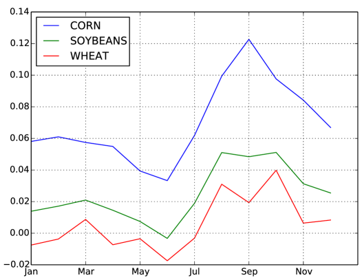
In order to develop tractable models with analytical solutions that are amenable to interpretation and calibration, we did not consider the seasonality of grain prices, among other features. To compare the basis over different months of the year, we illustrate in Figure 10 the average basis for all three commodities. As shown, the basis is typically higher during the fall harvest months (August to October) when available storage capacity is low and market storage rates are high. This suggests that the value of storage optionality, captured in our models here, is particularly high in these months. In contrast, the basis is typically smaller from the winter through the summer while the grain silos are being emptied before the next harvest, and thus, storage rates are reduced during the low season.

Overall, both of our proposed models are capable of generating model prices corresponding to a variety of market situations, such as high/low storage costs, and backwardated/contango futures curves, and fit well for different commodities. Therefore, the proposed models seem to have sufficient components and strong economic rationale to reflect and quantify non-convergence in the grains markets. There is certainly room for incorporating additional characteristics, such as seasonality and other contractual features, such as quality and delivery options. However, the relatively small number of traded futures contracts for each commodity may limit the number of model parameters, and thus, model sophistication.

A better understanding of the price behaviors of commodity futures is also relevant to broader financial market, especially in the current era of so-called financialization of the commodity market (see Tang and Xiong (2012)), whereby commodity prices have become more correlated with the equity market. Moreover, commodity futures also play a role in the exchange-traded fund (ETF) market since most commodity ETFs are essentially dynamic portfolios of commodity futures; see Guo and Leung (2015); Leung and Ward (2015), among others. Therefore, for investors seeking spot exposure through commodity ETFs, any model which sheds light on the non-convergence phenomenon will affect investment decisions.

While our models have both empirical explanatory power and theoretical foundation, our results do not rule out the possible scenario called the ‘failure of arbitrage’ in the grain markets, as suggested by the speculator hypothesis. Nevertheless, alternative theories of non-convergence can potentially be incorporated into our models. The unique feature of our models is the embedded double timing option. This should motivate future research to investigate the valuation of such a timing option under different stochastic storage rate dynamics. Other directions include adding to futures multiple options, such as the delivery option, quality option, and location option. Furthermore, we choose our models in this paper for analytical tractability which give closed-form certificate prices. One can also examine certificate prices under more complex stochastic models, for example, with stochastic interest rate, as well as stochastic volatility and jumps in the spot price or storage rate.

6 Appendix

6.1 Proofs: GBM with Stochastic Storage

6.1.1 Proposition 1

We derive the certificate price by first determining the liquidation value function $J(S_{\tau},\delta_{\tau})$ and then substituting the value to solve the certificate problem $V(S_{T},\delta_{T}).$ After applying the martingale property of $\left(M_{t}\right)_{t\geq 0}=\left(e^{-rt}S_{t}-\int_{0}^{t}\delta_{u}e^{-ru}du\right)_{t\geq 0}$, and applying the optional sampling theorem, the liquidation value function simplifies to

$$\begin{split}J(S_{\tau},\delta_{\tau})&=e^{r\tau}\left(\sup_{\eta\in\mathcal{T}_{\tau,\infty}}\mathbb{E}\left[e^{-r\eta}(S_{\eta}-c_{2})-\int_{\tau}^{\eta}\delta_{u}e^{-ru}du|\mathcal{F}_{\tau}\right]\right)\\ &=e^{r\tau}\left(\sup_{\eta\in\mathcal{T}_{\tau,\infty}}\mathbb{E}\left[M_{\eta}+\int_{0}^{\eta}\delta_{u}e^{-ru}du-\int_{\tau}^{\eta}\delta_{u}e^{-ru}du-c_{2}e^{-r\eta}|\mathcal{F}_{\tau}\right]\right)\\ &=e^{r\tau}\left(M_{\tau}+\int_{0}^{\tau}\delta_{u}e^{-ru}du+\sup_{\eta\in\mathcal{T}_{\tau,\infty}}\mathbb{E}\left[-c_{2}e^{-r\eta}|\mathcal{F}_{\tau}\right]\right)\\ &=S_{\tau}.\end{split}$$ (6.1)

From the last step, we see that $\eta=\infty$ is optimal. Furthermore, after substituting $J(S_{t},\delta_{t})=S_{t}$ into the certificate pricing problem, and again using the fact that $M_{t}$ is a martingale, we obtain a solution for $V(S_{T},\delta_{T})$ which is separable in $S_{T}$ and $\delta_{T}:$

$$V(S_{T},\delta_{T}) =e^{rT}\left(\sup_{\tau\in\mathcal{T}_{T,\infty}}\mathbb{E}\left[e^{-r\tau}(S_{\tau}-c_{1})-\int_{T}^{\tau}\widehat{\delta}e^{-ru}du|\mathcal{F}_{T}\right]\right)$$

$$=e^{rT}\left(M_{T}+\int_{0}^{T}\delta_{u}e^{-ru}du+\sup_{\tau\in\mathcal{T}_{T,\infty}}\mathbb{E}\left[\int_{T}^{\tau}(\delta_{u}-\widehat{\delta})e^{-ru}du-c_{1}e^{-ru}|\mathcal{F}_{T}\right]\right)$$

$$=S_{T}+\sup_{\tau\in\mathcal{T}_{T,\infty}}\mathbb{E}\left[\int_{T}^{\tau}(\delta_{u}-\widehat{\delta})e^{-r(u-T)}du-c_{1}e^{-r(\tau-T)}|\mathcal{F}_{T}\right].$$ (6.2)

We denote the second term in (6.2) by $P(\delta_{T})$, where the function $P(\delta)$ satisfies the variational inequality

$$\max\left\{\mathcal{L}P(\delta)-rP(\delta)+\delta-\widehat{\delta},-P-c_{1}\right\}=0,$$ (6.3)

where $\mathcal{L}\equiv\mathcal{L}^{\kappa,\nu,\zeta}$ is the infinitesimal generator defined in (3.8). In order to determine $P(\delta)$ and the optimal stopping strategy $\tau^{*},$ we first conjecture that $\tau^{*}$ takes the form

$$\tau^{*}=\inf\{t\geq T:\delta_{t}\leq\delta^{*}\}$$

for critical stopping level $\delta^{*}$ to be determined. In other words, when the market storage rate $\delta_{t}$ is sufficiently small, the agent exercises to take advantage of the cheaper market storage rate, instead of paying the higher certificate rate $\widehat{\delta}.$ Thus, for $\delta_{t}>\delta^{*}$, we look for the solution of the ODE $\mathcal{L}P(\delta)-rP(\delta)+\delta-\widehat{\delta}=0$, and for $\delta\leq\delta^{*}$ we require that $P(\delta)=-c_{1}$. This leads to the solution to the variational inequality

$$P(\delta)=\left[AH(\delta)+\frac{1}{\kappa+r}\left(\delta-\widehat{\delta}+\frac{\kappa(\nu-\widehat{\delta})}{r}\right)\right]\mathbf{1}\{\delta\geq\delta^{*}\}-c_{1}\mathbf{1}\{\delta<\delta^{*}\},$$ (6.4)

along with the boundary conditions: $P(\delta^{*})=-c_{1}$ and $P^{\prime}(\delta^{*})=0$. The latter is the smooth pasting condition, which implies that

$$A=-\frac{1}{H^{\prime}(\delta^{*})(\kappa+r)}.$$

Enforcing these boundary conditions together also yields the optimal exercise level $\delta^{*}$ in (3.15).

Consider the function defined from (3.15)

$$f(\delta^{*}):=\delta^{*}-\frac{H(\delta^{*})}{H^{\prime}(\delta^{*})}.$$ (6.5)

First, the properties of $H$ imply that ${H}/{H^{\prime}}\geq 0,$ so that $f(\delta^{*})\leq\delta^{*}$. Taking the limit as $\delta^{*}\to-\infty,$ we have $f(-\infty)=-\infty.$ Furthermore, under the restriction $\zeta^{2}\leq 2\kappa,$ and examining the terms inside the integrals of $H$ and $H^{\prime}$, namely,

$$H(\delta^{*}) =\int_{0}^{\infty}v^{\frac{r}{\kappa}-1}e^{\sqrt{\frac{2\kappa}{\zeta^{2}}}(x-\nu)v-\frac{v^{2}}{2}}dv,$$

$$H^{\prime}(\delta^{*}) =\int_{0}^{\infty}v^{\frac{r}{\kappa}}\sqrt{\frac{2\kappa}{\zeta^{2}}}e^{\sqrt{\frac{2\kappa}{\zeta^{2}}}(x-\nu)v-\frac{v^{2}}{2}}dv,$$

we conclude that $H/H^{\prime}\leq 1.$ Therefore, $f(\delta^{*})\geq\delta^{*}-1,$ and $f(\infty)=\infty.$ Finally, for $\delta^{*}\in(-\infty,\infty),$ $f^{\prime}={HH^{\prime}}/{H^{\prime\prime}}>0$. Therefore, we have

$$\lim_{\delta^{*}\to-\infty}f(\delta^{*})=-\infty,\qquad\lim_{\delta^{*}\to\infty}f(\delta^{*})=\infty,\qquad f^{\prime}(\delta^{*})>0.$$ (6.6)

The solution $\delta^{*}$ to (3.15) is unique.

6.2 Proofs: Exponential OU with Local Stochastic Storage

6.2.1 Proposition 2

We consider a candidate interval type strategy for both $\tau$ and $\eta$. First, since the certificate price is monotonically increasing in the spot price, we consider the optimal liquidation time $\eta^{*}$ to be of the form: $\eta^{*}=\inf\{t\geq\tau^{*}:U_{t}\geq u^{*}\}$. In the liquidation problem represented by $J$, we hold the commodity until the storage cost $\delta_{t}$, which is increasing in the commodity price $U_{t},$ is sufficiently large relative to the commodity price. We solve a variational inequality for the value function $J(u)$ and match the boundary condition at $u^{*}$ to get the solution. Assuming the conjectured form for $\eta^{*},$ $J(u)$ satisfies

$$\begin{cases}\mathcal{L}J(u)-rJ(u)=\beta u+\delta&\text{ if $u<u^{*}$},\\ J(u)=e^{u}-c_{2}&\text{ if }u\geq u^{*},\end{cases}$$ (6.7)

where $\mathcal{L}\equiv\mathcal{L}^{\alpha,\mu,\sigma}$ is the infinitesimal generator defined in (3.8). We apply the continuity and smooth pasting conditions to $J(u)$, and get

$$J(u^{*})=e^{u^{*}}-c_{2},\qquad J^{\prime}(u^{*})=e^{u^{*}},$$ (6.8)

This gives the solution (4.7) with $u^{*}$ satisfying

$$f(u^{*})=\frac{e^{u^{*}}+\beta/(\alpha+r)}{H^{\prime}(u^{*})}H(u^{*})-\frac{1}{\alpha+r}\left[\beta u^{*}+\gamma+\frac{\alpha(\beta\mu+\gamma)}{r}\right]-e^{u^{*}}+c_{2}=0.$$

When ${\sigma}<\sqrt{2\alpha}$, the level $u^{*}$ admits a unique solution. First we can write

$$f(u^{*})=e^{u^{*}}\left(\frac{H(u^{*})}{H^{\prime}(u^{*})}-1\right)+\frac{\beta}{\alpha+r}\left(\frac{H(u^{*})}{H^{\prime}(u^{*})}-u^{*}\right)+C,$$

for some constant C not depending on $u^{*}.$ Since $\frac{H}{H^{\prime}}\leq 1$ then $f(u^{*})\leq\frac{\beta}{\alpha+r}(1-u^{*})+C$ so $\lim_{u^{*}\to\infty}f(u^{*})=-\infty.$ Also, since $\frac{H}{H^{\prime}}\geq 0,$ then $f(u^{*})\geq-e^{u^{*}}-\frac{\beta}{\alpha+r}u^{*}+C$ so $\lim_{u^{*}\to-\infty}f(u^{*})=\infty.$ Finally, we can look at

$$f^{\prime}(u^{*})=-\frac{H(u^{*})}{H^{\prime}(u^{*})}\left[e^{u^{*}}\left(\frac{H^{\prime\prime}(u^{*})}{H^{\prime}(u^{*})}-1\right)+\frac{\beta}{\alpha+r}\frac{H^{\prime\prime}(u^{*})}{H^{\prime}(u^{*})}\right].$$

Using similar arguments as from the previous appendix, we canshow $\frac{H^{\prime\prime}}{H^{\prime}}\geq 1,$ so $f^{\prime}(u^{*})\leq-\frac{H(u^{*})}{H^{\prime}(u^{*})}\frac{\alpha}{\alpha+r}<0$ $\forall u^{*}\in\mathbb{R}.$ To recap, we have shown that

$$\lim_{u^{*}\to-\infty}f(u^{*})=\infty,\qquad\lim_{u^{*}\to\infty}f(u^{*})=-\infty,\qquad f^{\prime}(u^{*})<0,$$ (6.9)

so our solution $u^{*}$ is unique.

On the other hand, in the exercise problem $V$, the optimal strategy $\tau^{*}$ takes the form

$$\tau^{*}=\inf\{t\geq T:U_{t}\leq\underline{u}^{**}\text{ or }U_{t}\geq\overline{u}^{**}\},$$

In other words, hold the commodity until either (i) the storage cost is at or lower than $\underline{u}^{**}$ where the agent exercises, or (ii) the commodity price is reaches the upper level $\overline{u}^{**}$ at which the agent exercises $and$ liquidates. As such, the value function satisfies

$$\begin{cases}V(u)=e^{u}-c_{1}-c_{2}&\text{ if $u>\overline{u}^{**}$},\\ \mathcal{L}V(u)-rV(u)=\widehat{\delta}&\text{ if $\underline{u}^{**}\leq u\leq\overline{u}^{**}$},\\ V(u)=AH(u)-\frac{1}{\alpha+r}\left[\beta u+\delta+\frac{\alpha(\beta\mu+\delta)}{r}\right]-c_{1}&\text{ if $u<\underline{u}^{**}$}.\end{cases}$$ (6.10)

The boundary conditions for $\underline{u}^{**}$ and $\overline{u}^{**}$ are

$$\begin{split}V(\overline{u}^{**})&=e^{\overline{u}^{**}}-c_{1}-c_{2},\qquad V(\underline{u}^{**})=J(\underline{u}^{**})=AH(\underline{u}^{**})-\frac{1}{\alpha+r}\left[\beta\underline{u}^{**}+\delta+\frac{\alpha(\beta\mu+\delta)}{r}\right]-c_{1},\\ V^{\prime}(\overline{u}^{**})&=e^{\overline{u}^{**}},\qquad\qquad\qquad V^{\prime}(\underline{u}^{**})=J^{\prime}(\underline{u}^{**})=AH^{\prime}(\underline{u}^{**})-\frac{\beta}{\alpha+r}.\end{split}$$ (6.11)

We match the boundary conditions at $\underline{u}^{**}$ and $\overline{u}^{**}$ to get the solution (4.8).

References

- Adjemian et al. (2013) Adjemian, M. K., Garcia, P., Irwin, S., and Smith, A. (2013). Non-convergence in domestic commodity futures markets: causes, consequences, and remedies. USDA Economic Research Service, 115(155381).
- Aulerich et al. (2011) Aulerich, N. M., Fishe, R. P. H., and Harris, J. H. (2011). Why do expiring futures and cash prices diverge for grain markets? The Journal of Futures Markets, 31(6):503–533.
- Aulerich and Hoffman (2013) Aulerich, N. M. and Hoffman, L. A. (2013). Recent convergence performance of futures and cash prices for corn, soybeans and wheat. USDA Report from Economic Research Service, 13L(1).
- Biagini and Bjork (2007) Biagini, F. and Bjork, T. (2007). On the timing option in a futures contract. Mathematical Finance, 17(2):267–283.
- Borodin and Salminen (2002) Borodin, A. N. and Salminen, P. (2002). Handbook of Brownian Motion- Facts and Formulae. Birkhauser Verlag.
- Brennan (1958) Brennan, M. (1958). The supply of storage. American Economic Review, 48:50–72.
- Carmona and Coulon (2013) Carmona, R. and Coulon, M. (2013). A Survey of Commodity Markets and Structural Models for Electricity Prices. Springer New York.
- Deaton and Laroque (1996) Deaton, A. and Laroque, G. (1996). Competitive storage and commodity price dynamics. Journal of Political Economy, 104(5):896–293.
- Erdelyi and Tricom (1953) Erdelyi, Magnus, O. and Tricom (1953). Higher Transcendental Functions, volume 2. McGraw-Hill.
- Fama and French (1987) Fama, E. F. and French, K. R. (1987). Commodity futures prices: Some evidence on forecast power, premiums, and the theory of storage. The Journal of Business, 60(1):55–73.
- Garcia et al. (2014) Garcia, P., Irwin, S. H., and Smith, A. D. (2014). Futures market failure. American Journal of Agricultural Economics, 97(1):40–64.
- Gorton et al. (2012) Gorton, G. B., Hayashi, F., and Rouwenhorst, K. G. (2012). The fundamentals of commodity futures returns. Review of Finance, pages 31–105.
- Guo and Leung (2015) Guo, K. and Leung, T. (2015). Understanding the tracking errors of commodity leveraged ETFs. In Aid, R., Ludkovski, M., and Sircar, R., editors, Commodities, Energy and Environmental Finance, Fields Institute Communications, pages 39–63. Springer.
- Hinz and Fehr (2010) Hinz, J. and Fehr, M. (2010). Storage costs in commodity option pricing. SIAM Journal of Financial Math, 1(1):729–751.
- Hranaiova et al. (2005) Hranaiova, J., Jarrow, R. A., and Tomek, W. G. (2005). Estimating the value of delivery options in futures contracts. Journal of Financial Research, 28(3):363–383.
- Irwin et al. (2009) Irwin, S. H., Garcia, P., Good, D., and Kunda, E. (2009). Poor convergence performance of cbot corn, soybean and wheat futures contracts: Causes and solutions. Marketing and Outlook Research Report.
- Irwin et al. (2011) Irwin, S. H., Garcia, P., Good, D. L., and Kunda, E. L. (2011). Spreads and non-convergence in Chicago Board of Trade corn, soybean, and wheat futures: Are index funds to blame? Applied Economic Perspectives and Policy, 33(1):116–142.
- Johnson (1960) Johnson, L. L. (1960). The theory of hedging and speculation in commodity futures. The Review of Economic Studies, 27(3):139–151.
- Kaldor (1939) Kaldor, N. (1939). Speculation and economic stability. Review of Economic Studies, 7(1):1–27.
- Leung et al. (2016) Leung, T., Li, J., Li, X., and Wang, Z. (2016). Speculative futures trading under mean reversion. Asia-Pacific Financial Markets, 23(4):281–304.
- Leung and Li (2015) Leung, T. and Li, X. (2015). Optimal mean reversion trading with transaction costs and stop-loss exit. International Journal of Theoretical & Applied Finance, 18(3):15500.
- Leung and Li (2016) Leung, T. and Li, X. (2016). Optimal Mean Reversion Trading: Mathematical Analysis and Practical Applications. Modern Trends in Financial Engineering. World Scientific, Singapore.
- Leung et al. (2014) Leung, T., Li, X., and Wang, Z. (2014). Optimal starting–stopping and switching of a CIR process with fixed costs. Risk and Decision Analysis, 5(2):149–161.
- Leung et al. (2015) Leung, T., Li, X., and Wang, Z. (2015). Optimal multiple trading times under the exponential OU model with transaction costs. Stochastic Models, 31(4):554–587.
- Leung and Ward (2015) Leung, T. and Ward, B. (2015). The golden target: Analyzing the tracking performance of leveraged gold ETFs. Studies in Economics and Finance, 32(3):278–297.
- Tang and Xiong (2012) Tang, K. and Xiong, W. (2012). Index investment and the financialization of commodities. Financial Analysts Journal, 68(6):54–72.
- Working (1949) Working, H. (1949). The theory of the price of storage. American Economic Review, 39:1254–1262.