Inchworm Monte Carlo for exact non-adiabatic dynamics II. Benchmarks and comparison with established methods

Abstract

In this second paper of a two part series, we present extensive benchmark results for two different inchworm Monte Carlo expansions for the spin–boson model. Our results are compared to previously developed numerically exact approaches for this problem. A detailed discussion of convergence and error propagation is presented. Our results and analysis allow for an understanding of the benefits and drawbacks of inchworm Monte Carlo compared to other approaches for exact real-time non-adiabatic quantum dynamics.

I Introduction

The spin–boson model is perhaps the most basic example of a quantum dissipative system.Leggett et al. (1987) Despite its simplicity, the model endures for several reasons. First, the spin–boson rather faithfully represents the spectrum of realistic behaviors associated with the relaxation of a small quantum system connected to a heat bath.Weiss (1999) While the model employs seemingly unrealistic features such as linear coupling to a harmonic reservoir, even anharmonic systems may be mapped to this form of environmental interaction within linear response theory.Bader, Kuharski, and Chandler (1990); Warshel, Chu, and Parson (1989); Warshel and Hwang (1986); Makri (1999) This generality explains the wide usage of the spin–boson paradigm in the modeling of systems ranging from charge and energy transfer in condensed phases and biological systemsGarg, Onuchic, and Ambegaokar (1985); Georgievskii, Hsu, and Marcus (1999); Adolphs and Renger (2006); Engel et al. (2007); Lee, Cheng, and Fleming (2007); Panitchayangkoon et al. (2010); Collini and Scholes (2009); Brédas and Silbey (2009) to the relaxation of dilute impurities in the solid stateFisher and Zwerger (1985); Prokof’ev and Stamp (1996, 1998) and in Josephson junction arrays.Goldstein et al. (2013) In the rotating wave approximation, the spin–boson model is reduced to the Jaynes–Cummings model, which is of great importance in quantum optics.Fink et al. (2008); Solano, Agarwal, and Walther (2003); Casanova et al. (2010)

A second major reason for the continued study of the spin–boson model resides in the fact that it cannot be solved analytically and presents numerical challenges for exact quantum dynamics methodologies. Thus the model has become a canonical benchmark for both approximate and exact dynamical approaches. After approximately two decades of research, several numerically exact approaches have emerged which are capable of long-time simulation of time-dependent observables of the spin–boson Hamiltonian, at least for many important regimes of the model. These methods differ from one another with respect to their formulations, their scaling properties, their complexity and their generality. In this paper we will concern ourselves with benchmarks from three commonly used approaches: the quasi-adiabatic path integral (QUAPI) approach,Makarov and Makri (1994); Makri (1995); Makri and Makarov (1995); Makri et al. (1996) the hierarchical equations-of-motion (HEOM) method,Tanimura and Kubo (1989); Ishizaki and Fleming (2009); Strümpfer and Schulten (2012) and the multi-layer, multi-configuration time-dependent Hartree (ML-MCTDH) approach.Thoss, Wang, and Miller (2001); Wang, Thoss, and Miller (2001); Wang and Thoss (2003) There are fewer calculations of spin–boson dynamics done by stationary-phase Monte Carlo,Mak and Chandler (1990, 1991); Egger and Weiss (1992); Egger and Mak (1994); Egger, Mühlbacher, and Mak (2000) though this technique also yields numerically exact results.

We will focus on diagrammatic Monte Carlo methods,Prokof’ev and Svistunov (1998, 2008a, 2008b); Van Houcke et al. (2010) a dominant and widely applicable formalism for addressing impurity models. These methods allow for facile computation of equilibrium observables in general impurity-type problems,Gull et al. (2011) including those unrelated to the spin–boson model. They have also been used for non-equilibrium problems,Mühlbacher and Rabani (2008); Werner, Oka, and Millis (2009); Cohen et al. (2014a, b, 2013) where they are limited in applicability by the dynamical sign problem. Recently, we have introduced an exact, real-time diagrammatic Monte Carlo approach called the inchworm algorithmCohen et al. (2015) which greatly suppresses the dynamical sign problem. In the companion paper to the work presented here, we have elaborated upon and expanded the scope of the approach, using the spin–boson model as a concrete example.

In this work we compare the results of the inchworm algorithm to those produced by the other methodologies mentioned above in essentially all regimes of interest. Our results allow us to compare and contrast the strengths and weaknesses of the relative approaches. We demonstrate that the inchworm algorithm is competitive with the most advanced real-time approaches and is capable of producing converged long-time results even in some regimes difficult for several prominent approaches. The success of the inchworm algorithm as outlined in this work paves the way for a host of novel applications, a few of which we enumerate at the conclusion of this paper.

The paper is organized as follows. In Sec. II, we specify details of the spin–boson model and provide an analysis of convergence for the system–bath coupling inchworm (SBCI) and the diabatic coupling cumulant inchworm (DCCI) approaches. In Sec. III, we present a detailed comparison of our new approaches to established benchmarks, as well as a discussion of the relative benefits and drawbacks of our approach in comparison to established methods. Our conclusions are presented in Sec. IV.

II Model and methods

To avoid redundancy with the companion paper, we only include specific details needed for the following discussion. In particular, we specify the particular form of the spectral density and provide a detailed analysis of the convergence properties for both the DCCI and the SBCI.

II.1 Spin–boson model and parameters

We set $\hbar=1$ and consider a spin–boson Hamiltonian of the form

$$H=\epsilon\hat{\sigma}_{z}+\Delta\hat{\sigma}_{x}+\hat{\sigma}_{z}\sum_{\ell}c_{\ell}x_{\ell}+\sum_{\ell}\frac{1}{2}\left(p_{\ell}^{2}+\omega_{\ell}^{2}x_{\ell}^{2}\right),$$ (1)

where the $\hat{\sigma}_{i}$ are Pauli matrices describing the spin, and the parameters $\varepsilon$ and $\Delta$ are called the bias and diabatic coupling, respectively. The $x_{\ell}$ and $p_{\ell}$ are boson operators. Throughout this work, we specify the system–bath coupling strength, which determines the $c_{\ell}$ and $\omega_{\ell}$, by a spectral density that is linear for small $\omega$ and has a Lorentzian cutoff for large $\omega$:

$$J_{D}\left(\omega\right)=\frac{\lambda}{2}\frac{\omega_{c}\omega}{\omega_{c}^{2}+\omega^{2}}.$$ (2)

This is known in the literature as the Debye spectral density.Weiss (1999) The reorganization energy, defined as $\lambda=\frac{4}{\pi}\int\frac{J\left(\omega\right)}{\omega}d\omega=2\sum_{\ell}c_{\ell}^{2}/\omega_{\ell}^{2}$, sets the maximal system–bath coupling strength. The cutoff frequency of the Lorentzian function, $\omega_{c}$, characterizes the band width of the bath. Therefore, at equilibrium, the version of the spin–boson model we consider is fully characterized by five parameters: the diabatic coupling $\Delta$, the bias energy $\epsilon$, the cut-off frequency $\omega_{c}$, the reorganization energy $\lambda$, and the temperature $k_{B}T=1/\beta$ of the boson bath ($k_{B}$ is Boltzmann constant).

We assume a factorized initial condition given by $\rho_{0}=\rho_{s}\otimes\rho_{b}$. The initial condition of the spin is $\rho_{s}=\left|1\right\rangle\left\langle 1\right|$, and the initial density matrix of the bath is thermal equilibrium in the absence of the system–bath coupling,

$$\rho_{b}=\frac{e^{-\beta H_{b}}}{\mathrm{Tr}_{b}\left\{e^{-\beta H_{b}}\right\}}.$$ (3)

This is where the dependence on (inverse) temperature $\beta$ appears. We will concentrate on the local dynamics of the spin operator $\sigma_{z}$,

$$\left\langle\sigma_{z}\left(t\right)\right\rangle=\mathrm{Tr}\left\{\rho_{0}e^{iHt}\hat{\sigma}_{z}e^{-iHt}\right\},$$ (4)

which is often referred to the “population difference” of the spin.

II.2 Convergence analysis

To obtain a simple estimate for how rapidly the inchworm approaches are expected to converge in different regions of parameter space, we focus on the lowest-order nontrivial contribution in each type of expansion and determine its magnitude as a function of model parameters. We consider the $2^{\mathrm{nd}}$-order term of the SBCI and DCCI expansions, which in both cases can be written in the form

$$G_{2}\left(t\right)=\int_{0}^{t}\mathrm{d}t_{1}\int_{0}^{t_{2}}\mathrm{d}t_{2}C\left(t_{1},t_{2}\right).$$ (5)

Here, $C\left(t_{1},t_{2}\right)$ is the bath correlation function associated with each expansion. Loosely speaking, one might expect an expansion to converge rapidly as long as the corresponding $G_{2}\left(t\right)$ is not significantly greater than unity. Given the functional form of the Debye spectral density, we can easily evaluate $G_{2}\left(t\right)$ in an analytical or semi-analytical fashion (i.e. by numerical quadrature).

For the SBCI expansion, we can evaluate $G_{2}\left(t\right)$ in the high and low temperature limits and then derive the convergence conditions from the appropriate dimensionless parameters that emerge. This scheme is analogous to one which has been used to determine the limitations of Redfield theory.Montoya-Castillo, Berkelbach, and Reichman (2015) The bath correlation function in the SBCI expansion is given by $C\left(t_{1},t_{2}\right)=\left\langle\widetilde{B}\left(t_{1}\right)\widetilde{B}\left(t_{2}\right)\right\rangle_{b}$ where $\widetilde{B}\left(t\right)=\sum_{\ell}c_{\ell}\widetilde{x}_{\ell}\left(t\right)$, and with the definition $\left\langle\cdot\right\rangle_{b}\equiv\mathrm{Tr}_{b}\left\{\rho_{b}\cdot\right\}$. The explicit expression is derived in Eq. (31) of the companion paper:

$$\begin{split}&\left\langle\widetilde{B}\left(t_{1}\right)\widetilde{B}\left(t_{2}\right)\right\rangle_{b}=\frac{2}{\pi}\int d\omega J_{D}\left(\omega\right)\times\\ &\ \left[\coth\left(\frac{\beta\omega}{2}\right)\cos\omega\left(t_{1}-t_{2}\right)-i\sin\omega\left(t_{1}-t_{2}\right)\right].\end{split}$$ (6)

The integral takes the form $G_{2}\left(t\right)=\xi g\left(t\right)$, where $\xi$ is a dimensionless parameter and $g\left(t\right)$ is a time-dependent dimensionless function. We expect the expansion to converge rapidly as long as $\xi\lesssim 1$. In the high temperature limit $\beta\text{$\omega$}_{c}\ll 1$, and we can approximate $\coth\left(\frac{\beta\omega}{2}\right)\approx\frac{2}{\beta\omega}$ and obtain the dimensionless form for $\xi$:

$$\xi=\frac{\lambda}{\beta\omega_{c}^{2}}-i\frac{\lambda}{2\omega_{c}}.$$ (7)

Thus, in this regime, an estimate for the condition for convergence of the SBCI approach is

$$\frac{\lambda}{\beta\omega_{c}^{2}}\apprle 1.$$ (8)

In the low temperature limit $\beta\text{$\omega$}_{c}\gg 1$, we can use $\coth\left(\frac{\beta\omega}{2}\right)\approx 1$, but cannot carry out the integral analytically. In the same spirit, we factor out the dimensionless scale of the integral, $\mathrm{Re}\left[G_{2}\left(t\right)\right]=\frac{\lambda}{\pi\omega_{c}}\int\mathrm{d}x\frac{1}{x^{2}+1}\frac{1}{x}\left(1-\cos\omega_{c}xt\right)$, which yields a convergence condition for the low temperature limit

$$\frac{\lambda}{\pi\omega_{c}}\apprle 1.$$ (9)

It is noteworthy that since $G_{2}\left(t\right)$ is proportional to $\lambda\coth\left(\beta\omega/2\right)$, the SBCI expansion becomes more difficult to converge as $\lambda$ increases or $\beta$ decreases.

The explicit form of the bath correlation function in the DCCI expansion is given by $C\left(t_{1},t_{2}\right)=e^{-4{\cal Q}_{2}\left(t_{1}-t_{2}\right)-i4{\cal Q}_{1}\left(t_{1}-t_{2}\right)}$, where

$${\cal Q}_{1}\left(t\right)=\frac{2}{\pi}\int\mathrm{d}\omega\frac{J_{D}\left(\omega\right)}{\omega^{2}}\sin\omega t,$$ (10)

$${\cal Q}_{2}\left(t\right)=\frac{2}{\pi}\int\mathrm{d}\omega\frac{J_{D}\left(\omega\right)}{\omega^{2}}\coth\left(\frac{\beta\omega}{2}\right)\left(1-\cos\omega t\right).$$ (11)

Due to the complicated form of these correlation functions, one cannot obtain an analytical expression to extract a dimensionless scale parameter. Therefore, we evaluate the integral numerically at a large enough time for given model parameters. Note that the subsequent discussion for the convergence condition is obtained by carrying out the integral numerically. We also note that ${\cal Q}_{1}$ and ${\cal Q}_{2}$ are linearly dependent on $\lambda$, which yields a $1/\lambda^{2}$ dependence for $G_{2}\left(t\right)$. Therefore, the DCCI expansion becomes easier to converge as $\lambda$ increases.

(a) $\beta\Delta=0.5$

(b) $\beta\Delta=5$

(c) $\beta\Delta=50$

Figure 1: Spin–boson model parameter space with zero bias $\epsilon=0$. The $x$-axis is $\lambda/\Delta$ in $\log$ scale and the $y$-axis is $\omega_{c}/\Delta$ in linear scale. The bath temperatures are (a) $\beta\Delta=0.5$, (b)$\beta\Delta=5$, and (c) $\beta\Delta=50$. In each “phase diagram”, the estimated region of rapid convergence for the SBCI approach is to the left of the dashed line (red) and is to the right of the dotted line (blue) for the DCCI approach. Points indicate the parameters for plots presented in this work.

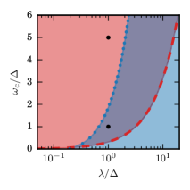
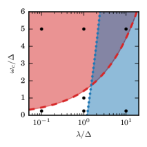
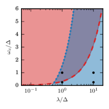
A two-dimensional “phase diagram” can be drawn as cuts of the full parameter space with varying $\lambda$ and $\omega_{c}$, shown in Fig. 1. Here we limit the discussion to the subspace with zero energy bias $\epsilon=0$. The horizontal axis is the scaled reorganization energy ($\lambda/\Delta$) in $\log$ scale and the vertical axis is the scaled cutoff frequency ($\omega_{c}/\Delta$). Within this coordinate system, we can demarcate the estimated region of facile convergence for the SBCI and DCCI expansions by the conditions given above. The red regions indicate the subspace satisfying Eq. (8) and (9), in which the SBCI approach is expected to converge rapidly. The blue regions are obtained by semi-analytical estimation of the analogous condition for the DCCI approach.

Fig. 1 exhibits these complementary regions and shows that their combined area covers much of the relevant parameter space. We will briefly point out some important features of the phase diagram. First, for any cutoff frequency $\omega_{c}$, the SBCI converges better in the small $\lambda$ direction while the DCCI is expected to work better as $\lambda$ increases. Second, the region of utility for the SBCI expansion shrinks in the adiabatic regime (small $\omega_{c}$), which is due to the fact that the correlation functions in the SBCI expansion have a longer correlation time when $\omega_{c}$ is small. Lastly, as the temperature decreases, the regions of rapid convergence of both the SBCI and DCCI approaches expand and cover almost the entire parameter space.

While Fig. 1 provides an illustration of applicable regions of our approach, the regions are determined by rough estimation of lowest order contribution. In principle, our inchworm expansions are numerically exact in the entire parameter space, as discussed in the companion paper. In the “uncovered” or white region, our approaches should continue to yield reliable dynamical behavior at least on some time scales, albeit with potentially much greater numerical effort.

III Results

III.1 Computational Methodology

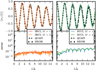
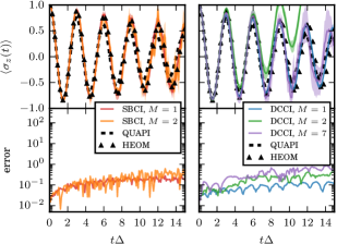
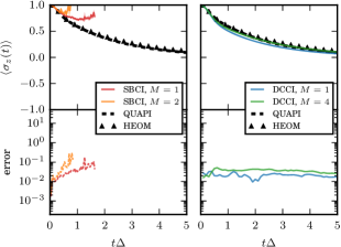
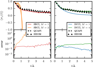
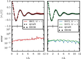
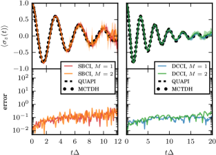
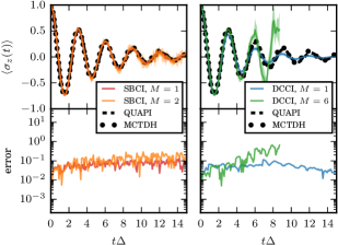
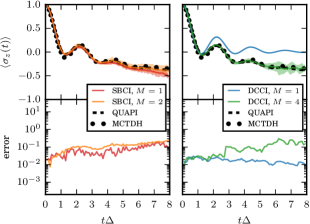
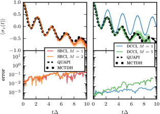
The general framework of the two general types of inchworm expansions used here may be found in the companion paper. In the following, each inchworm step is limited to a fixed run time and the order of each individual inchworm diagram is restricted to a maximum order $M$. We use $\mathrm{d}t\Delta=0.1$ for the size of the inchworm step in the following calculation, unless otherwise specified. One may then check for convergence by systematically increasing $M$, decreasing $\mathrm{d}t$ and increasing the number of Monte Carlo samples.Cohen et al. (2015) The SBCI calculation requires the full information contained in two-time restricted propagators, thus for the SBCI propagation to a time $t=N\mathrm{d}t$ requires $N^{2}$ inchworm steps (in fact, by taking advantage of time-reversal symmetry and the contour ordering of the time arguments, the number of steps needed turns out to be $\sim\frac{1}{4}N^{2}$). On the other hand, the DCCI expansion is phrased solely in terms of single-time properties, such that it requires only $N$ inchworm steps to reach a simulation time $t=N\mathrm{d}t$. For both approaches, we perform multiple independent inchworm calculations in order to properly account for error propagation.Cohen et al. (2015) Note that the error propagation shown in the lower subplot of all the figures is this “full” error, except for the left panels in Fig 3, where the standard Monte Carlo statistical error is shown for didactic purposes.

We compare our calculations with several existing numerically exact methods, including the quasi-adiabatic propagator path integral (QUAPI),Makarov and Makri (1994); Makri (1995); Makri and Makarov (1995); Makri et al. (1996) hierarchical equations of motion (HEOM) method,Tanimura and Kubo (1989); Ishizaki and Fleming (2009); Strümpfer and Schulten (2012) and the multi-configuration time-dependent Hartree (MCTDH) approach.Thoss, Wang, and Miller (2001); Wang, Thoss, and Miller (2001); Wang and Thoss (2003) QUAPI is based on the discretization of influence functional for reduced propagation on the Keldysh contour. The maximum number of short-time propagators that the path integral spans is determined by a parameter $k_{\mathrm{max}}$, which governs the memory length. The approach becomes difficult to converge when the memory length is long. The HEOM approach introduces a hierarchy of auxiliary density matrices and employs a Mastsubara expansion for the bath density matrix. The hierarchy truncation level $L$ and number of Matsubara terms $K$ are numerical parameters that are tuned to converge the HEOM calculation. A standard, highly parallel implementation is available,Strümpfer and Schulten (2012) known to be accurate in the high temperature limit and for the Debye spectral density. Generically, the HEOM approach has more difficulty for low temperatures and non-Debye spectral densities. The MCTDH approach is based on the expansion of the interacting many-body wave function as a tensor product of wavefunctions defined in a convenient set of orbitals. A highly efficient protocol may then be used to control, in a time-dependent manner, the number of orbitals needed for exact convergence. Exact MCTDH results for the spin–boson model are reported in Ref. Thoss, Wang, and Miller, 2001.

We will be using the benchmarks to investigate accuracy, and will make no attempt to compare numerical efficiency beyond general points having to with the computational scaling of the algorithms. To provide a general idea, we will say that using our current implementation, most of the (linear scaling in time) DCCI results presented here can be comfortably obtained on a laptop in minutes to hours, whereas the (quadratically scaling in time) SBCI results typically require a small cluster. However, it should be noted that the data below was obtained with a very flexible but not at all optimized code written in the high-level Python programming language. From our experience with similar algorithms for the Anderson impurity model,Cohen et al. (2015) we estimate that 1–2 orders of magnitude in overall runtime could be achieved by writing an efficient code, or simply by switching to a compiled language.

III.2 High temperature regime

(a) $\lambda/\Delta=0.1$, $\omega_{c}/\Delta=5$

(b) $\lambda/\Delta=0.1$, $\omega_{c}/\Delta=0.25$

Figure 2: Nonequilibrium population difference $\left\langle\sigma_{z}\left(t\right)\right\rangle$ (top subplots) and corresponding error estimates (bottom subplots) as a function of time in the weak coupling ($\lambda/\Delta=0.1$) and high temperature ($\beta\Delta=0.5$) regime. The bias energy is $\epsilon=0$. The results calculated by the SBCI (left panels, red and orange) and DCCI (right panels, blue and green) inchworm expansions are plotted for (a) a non-adiabatic (fast) bath with $\omega_{c}/\Delta=5$, and (b) an adiabatic (slow) bath with $\omega_{c}/\Delta=0.25$. Maximum order for an inchworm step is indicated by $M$. The thickness of the Monte Carlo results results from our error estimates. The dashed lines are the QUAPI results with (a)$\Delta t=0.1$, $k_{\mathrm{max}}=6$ and (b)$\Delta t=0.1$, $k_{\mathrm{max}}=12$. The triangles indicate the HEOM result with $K=2$ and $L=20$.

(a) $\lambda/\Delta=10$, $\omega_{c}/\Delta=5$

(b) $\lambda/\Delta=10$, $\omega_{c}/\Delta=0.25$

Figure 3: Nonequilibrium population difference $\left\langle\sigma_{z}\left(t\right)\right\rangle$ (top subplots) and corresponding error estimates (bottom subplots) as a function of time in the strong coupling ($\lambda/\Delta=10$) and high temperature ($\beta\Delta=0.5$) regime. The bias energy is $\epsilon=0$. The results calculated by the SBCI (left panels, red and orange) and DCCI (right panels, blue and green) inchworm expansions are plotted for (a) a non-adiabatic (fast) bath with $\omega_{c}/\Delta=5$, and (b) an adiabatic (slow) bath with $\omega_{c}/\Delta=0.25$. The time step of SBCI for (a) is $\mathrm{d}t\Delta=0.1/3$. The error estimate of the SBCI calculation (dashed lines in red and organe) is for one single run. Maximum order for a inchworm step is indicated by $M$. The thickness of the Monte Carlo results results from our error estimates. The dashed lines are the QUAPI results with (a)$\Delta t=0.1$, $k_{\mathrm{max}}=6$ and (b)$\Delta t=0.3$, $k_{\mathrm{max}}=11$. The triangles indicate the HEOM result with $K=2$ and $L=20$.

(a) $\lambda/\Delta=1$, $\omega_{c}/\Delta=5$

(b) $\lambda/\Delta=1$, $\omega_{c}/\Delta=1$

(c) $\lambda/\Delta=1$, $\omega_{c}/\Delta=0.25$

Figure 4: Nonequilibrium Population difference $\left\langle\sigma_{z}\left(t\right)\right\rangle$ (top subplots) and corresponding error estimates (bottom subplots) as a function of time in the intermediate coupling ($\lambda/\Delta=1$) and high temperature ($\beta\Delta=0.5$) regime. The bias energy is $\epsilon=0$. The results calculated by the SBCI (left panels, red and orange) and DCCI (right panels, blue and green) expansions are plotted for (a) a non-adiabatic (fast) bath with $\omega_{c}/\Delta=5$, (b) an intermediate bath with $\omega_{c}/\Delta=1$, and (c) an adiabatic (slow) bath with $\omega_{c}/\Delta=0.25$. Maximum order for a inchworm step is indicated by $M$. The thickness of the Monte Carlo results results from our error estimates. The dashed line are the QUAPI results with (a) $\Delta t=0.1$, $k_{\mathrm{max}}=6$, (b) $\Delta t=0.2$, $k_{\mathrm{max}}=10$, and (c) $\Delta t=0.3$, $k_{\mathrm{max}}=11$. The triangles indicate the HEOM result with $K=2$ and $L=20$.

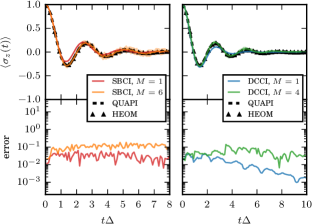
We start our comparison of the inchworm approaches with other exact methods in the high temperature regime (Fig. (1)(a)), specifically $\beta\Delta=0.5$ ($k_{B}T/\Delta=2$), and consider the vertical cuts at weak coupling $\lambda/\Delta=0.1$, strong coupling $\lambda/\Delta=10$, and intermediate coupling $\lambda/\Delta=1$ in the following.

III.2.1 Weak coupling

In the weak system–bath coupling regime, we consider cases with scaled reorganization energy ($\lambda/\Delta=0.1$) where we expect the SBCI expansion to converge more easily than the DCCI expansion. In Fig. 2, we find that the lowest order ($M=1$) results for the SBCI expansion always gives a quantitative account of the dynamics with the error remaining nearly constant over the simulation time. The SBCI result also converges rapidly upon increasing the maximum order $M$ of each inchworm step. We note that a smaller cut-off frequency yields a greater statistical error (see the lower panels of Fig. 2(a) and (b)) with the same computational cost. This is due to the long correlation time induced by a small $\omega_{c}$, which makes it more difficult to converge the SBCI expansion. On the other hand, the DCCI calculation also yields surprisingly accurate results. However, for a small cut-off frequency, it becomes more difficult to converge the DCCI approach, as can be seen in the right panel of Fig.2(b). Note that for the DCCI approach, convergence is non-monotonic: whereas the $M=1$ case appears quite accurate, the $M=2$ case actually yields results that are substantially worse. To overcome this, it is necessary to include much higher order inchworm diagrams. In this case $M=7$ appears to be sufficient. When many contributions at high orders are important, a larger investment of computer time is generally required to overcome the sign problem (here, ~3 times more computing resources were used to obtain the still noisy $M=7$ result than was used for $M=1$ and $M=2$).

Thus, in the high temperature, weak coupling regime, both inchworm approaches appear capable of reproducing the results obtained by the HEOM method, which easily converges to the exact answer for the Debye spectral density at high temperatures. The DCCI approach does show some convergence difficulties in this regime for the slow bath case. We could not converge QUAPI in the slow bath regime, and quantitative discrepancies can be found between QUAPI and HEOM here, as seen in Fig. 2.

III.2.2 Strong coupling

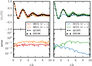
For strong system–bath coupling ($\lambda/\Delta=10$), we anticipate that the SBCI expansion will be difficult to converge and the DCCI expansion will show rapid convergence. The right panels of Fig. 3(a) and (b) show that the DCCI results converge to accurate population dynamics as we increase the maximum order $M$ of each inchworm step, but that at least $M=4$ is required for convergence. As expected, the SBCI expansion is difficult to converge in this parameter regime. The origins of this convergence issue can be gleaned from the behavior of the error estimate. In particular, the error estimates found in the left panels in Fig. 3 show the statistical error for one single SBCI calculation, which indicates the error of the Monte Carlo estimation of the integral within each inchworm step. This is an underestimate of the error margin, as it does not take into account the error propagation from shorter times; other plots in this paper show the full error analysis. We note that even the single run error increases exponentially with time, so that it is clear that the origin of the exponential growth in noise to signal ratio is actually the sign problem and not error propagation. The weight of high order configurations to the integral becomes large when $\lambda$ increases, and the SBCI expansion could not be converged in Fig. 3(a) even with a third of the inchworm step size used in the rest of the figures in this paper. To capture these high order contributions, one may increase $M$. However, as shown in Fig. 3, the slope of the statistical error grows unfavorably in this case as we increase $M$, rendering the SBCI expansion difficult to converge. This is the only part of the parameter space where we have found that one of the two methods proposed in the companion paper completely fails to overcome the dynamical sign problem.

We also note that the full error may not always monotonically increase with time and can exhibit decreasing or non-monotonic behavior. This is due to the fact that all contributions are dressed with full propagators tailored to the observable being measured. Where the value of the observable is small, each and every contribution will therefore be composed of small propagators and tend to be accordingly small, such that the statistical noise obtained is proportional to the (absolute) value at the point being measured.

III.2.3 Intermediate coupling

Lastly, we focus on the intermediate system–bath coupling regime where the scaled reorganization energy is $\lambda/\Delta=1$. Fig. 4 exhibits a general feature of the inchworm approaches: convergence with respect to the maximum order becomes more difficult to obtain as the cut-off frequency decreases. For a fast bath ($\omega_{c}/\Delta=5$), both the SBCI and DCCI expansions yield quite accurate results at lowest order. For $\omega_{c}/\Delta=1$, the parameter set $\left(\lambda/\Delta,\omega_{c}/\Delta\right)=\left(1,1\right)$ is located outside of the “safe” regions for the SBCI and DCCI as demarcated in Fig. 1(a). Here we observe clear, but small, discrepancies between the SBCI/DCCI results for $M=1$ and numerically exact dynamics. By systematically increasing $M$, the discrepancies can be corrected. When the cut-off frequency is small, the parameter set $\left(\lambda/\Delta,\omega_{c}/\Delta\right)=\left(1,0.25\right)$ is particularly difficult for both SBCI and DCCI expansions, although convergence is still seen for $M=6$. Lastly, note that here, as in Fig. 3, some notable discrepancies exist between the HEOM and QUAPI results. The inchworm expansions always converge to the HEOM results, which are expected to be more reliable in the high temperature regime.

III.3 Low temperature regime

We now turn our attention to the phase diagram in the low temperature regime, specifically $\beta\Delta=5$ ($k_{B}T/\Delta=0.2$), and concentrate on vertical cuts at intermediate coupling $\lambda/\Delta=1$ and strong coupling $\lambda/\Delta=10$, using the more suitable of the two methods in each case. These parameters correspond to Fig. 1(b).

III.3.1 Intermediate coupling

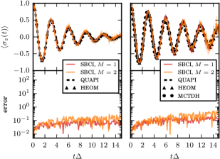
For intermediate coupling strength ($\lambda/\Delta=1$), the SBCI expansion is expected to converge at low temperatures more easily than in the high temperature regime. In particular, Fig. 1 shows the region of rapid convergence for the SBCI expansion becomes larger at low temperatures (b) than high temperatures (a). In Fig. 5, we find that the SBCI expansion can provide accurate results even at $M=1$ for the parameter sets $\left(\lambda/\Delta,\omega_{c}/\Delta\right)=\left(1,1\right)$ and $\left(1,0.25\right)$, which would be more difficult to converge in the high temperature regime discussed in Sec. III.2.

(a)$\lambda/\Delta=1$, $\omega_{c}/\Delta=1$     (b)$\lambda/\Delta=1$, $\omega_{c}/\Delta=0.25$

Figure 5: Nonequilibrium Population difference $\left\langle\sigma_{z}\left(t\right)\right\rangle$ (top subplots) and corresponding error estimates (bottom subplots) as a function of time in the intermediate coupling ($\lambda/\Delta=1$) and low temperature ($\beta\Delta=5$) regime. The bias energy is $\epsilon=0$. The results calculated by the SBCI (red lines) expansions are plotted for (a) an intermediate bath with $\omega_{c}/\Delta=1$ and (b) an adiabatic bath with $\omega_{c}/\Delta=0.25$. The maximum order for the inchworm step shown is $M=1$. The thickness of the Monte Carlo results results from our error estimates. The dashed lines are the QUAPI results with (a) $\Delta t=0.1$, $k_{\mathrm{max}}=6$ and (b) $\Delta t=0.1$, $k_{\mathrm{max}}=10$. The triangles indicate the HEOM result with $K=2$ and $L=20$. The MCTDH data is reported in Ref. Thoss, Wang, and Miller, 2001.

III.3.2 Strong coupling

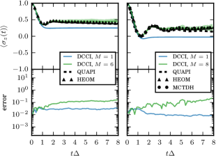
In the strong coupling regime ($\lambda/\Delta=10$), the DCCI approach is more rapidly convergent and efficient than the SBCI expansion (see Fig. 6). In particular, we show the DCCI results for parameter sets in the adiabatic and intermediate regime, namely $\left(\lambda/\Delta,\omega_{c}/\Delta\right)=\left(10,1\right)$ and $\left(10,0.25\right)$. In these regimes, the lowest order DCCI results tend to over-estimate the incoherent decay of the population. Including higher order contributions within each inchworm step is necessary, as it provides significant corrections to population dynamics leading to agreement with the HEOM and MCTDH results. At small $\omega_{c}/\Delta$, one needs to go as far as $M=8$, which is too difficult to fully converge with our current prototype code without spending a great deal of computer time. In the adiabatic regime (small $\omega_{c}$), QUAPI also tends to overestimate the decay for the long time behavior. To obtain correct long-time dynamics, one would need to increase the truncation of the memory length $k_{\mathrm{max}}$, which greatly increases the need for memory and makes QUAPI difficult to converge.

(a)$\lambda/\Delta=10$, $\omega_{c}/\Delta=1$      (b)$\lambda/\Delta=10$, $\omega_{c}/\Delta=0.25$

Figure 6: Nonequilibrium Population difference $\left\langle\sigma_{z}\left(t\right)\right\rangle$ (top subplots) and corresponding error estimates (bottom subplots) as a function of time in the strong coupling ($\lambda/\Delta=10$) and low temperature ($\beta\Delta=5$) regime. The bias energy is $\epsilon=0$. The results calculated by the DCCI (blue and green lines) expansions are plotted for (a) an intermediate bath with $\omega_{c}/\Delta=1$ and (b) an adiabatic bath with $\omega_{c}/\Delta=0.25$. Maximum order for a inchworm step is indicated by $M$. The thickness of the Monte Carlo results results from our error estimates. The dashed line are the QUAPI results with (a) $\Delta t=0.2$, $k_{\mathrm{max}}=11$ and (b) $\Delta t=0.4$, $k_{\mathrm{max}}=10$. The triangles indicate the HEOM result with $K=3$ and $L=20$. The MCTDH data is reported in Ref. Thoss, Wang, and Miller, 2001.

III.4 Very low temperature limit

Finally, we explore the very low temperature limit $\beta\Delta=50$ ($k_{B}T/\Delta=0.02$) corresponding to the phase diagram Fig. 1(c). In this limit, the standard HEOM implementationStrümpfer and Schulten (2012) can be computationally expensive to converge. Indeed, the lower the bath temperature, the more Matsubara terms that are needed to capture the bath density matrix and the more hierarchical levels are required to converge the long-time dynamics. We find that the HEOM implementation available to us becomes unfeasible for very low temperatures, though we note that recent advances may ameliorate this problem in at least some instances.Hu, Xu, and Yan (2010); Hu et al. (2011); Yan (2014); Moix and Cao (2013); Tang et al. (2015); Ye et al. (2016) At least in the Anderson model, this is not always the case.Härtle et al. (2015) Fig. 1 suggests that the SBCI and DCCI expansions hold an advantage over HEOM (though not MCTDH) at low temperatures, in that the computational cost does not increase with decreasing temperature. However, since at low enough temperatures strong correlation effects may alter the picture, it is not trivial that the simple analysis used to generate this figure should hold.

In Fig. 1(c), the combined area of strong convergence for the SBCI and DCCI expansions covers almost the entire parameter space in the very low temperature case. For the fast bath case ($\omega_{c}/\Delta=5$), Fig. 7(a) shows that the parameter set falls out of the region of facile convergence for the DCCI approach, however we find that the DCCI expansion can still provide accurate population dynamics, and is in fact more efficient than the SBCI expansion. On the other hand, for the intermediate cut-off frequency case ($\omega_{c}/\Delta=1$), the SBCI expansion results in population dynamics that agree perfectly with the MCTDH result, while we note that the DCCI expansion is difficult to converge with respect to the maximum order $M$ (see Fig. 7(b)). This clearly does not agree with our naive estimates for convergence of the DCCI expansion.

(a) $\lambda/\Delta=1$, $\omega_{c}/\Delta=5$, $\beta\Delta=50$

(b) $\lambda/\Delta=1$, $\omega_{c}/\Delta=1$, $\beta\Delta=50$

Figure 7: Nonequilibrium population difference $\left\langle\sigma_{z}\left(t\right)\right\rangle$ (top subplots) and corresponding error estimates (bottom subplots) as a function of time in the intermediate coupling ($\lambda/\Delta=1$) and very low temperature ($\beta\Delta=50$) regime. The bias energy is $\epsilon=0$. The results calculated by the SBCI (left panels) and the DCCI (right panels) expansions are plotted for (a) a non-adiabatic (fast) bath with $\omega_{c}/\Delta=5$ and (b) an intermediate bath with $\omega_{c}/\Delta=1$. Maximum order for each inchworm step is indicated by $M$. The thickness of the Monte Carlo results results from our error estimates. The dashed line are the QUAPI results with $\Delta t=0.1$ and $k_{\mathrm{max}}=10$. The MCTDH data is reported in Ref. Thoss, Wang, and Miller, 2001.

III.5 Biased systems

(a) $\lambda/\Delta=1$, $\omega_{c}/\Delta=5$, $\beta\Delta=0.5$

(b) $\lambda/\Delta=1$, $\omega_{c}/\Delta=5$, $\beta\Delta=50$

Figure 8: Nonequilibrium population difference $\left\langle\sigma_{z}\left(t\right)\right\rangle$ (top subplots) and corresponding error estimates (bottom subplots) as a function of time in the intermediate coupling ($\lambda/\Delta=1$) and non-adiabatic ($\omega_{c}/\Delta=5$) regime. The bias energy is $\epsilon=\Delta$. The results calculated by the SBCI (left panels) and the DCCI (right panels) expansions are plotted for (a) high temperature with $\beta\Delta=0.5$ and (b) very low temperature with $\beta\Delta=50$. Maximum order for each inchworm step is indicated by $M$. The thickness of the Monte Carlo results results from our error estimates. The dashed line are the QUAPI results with $\Delta t=0.1$ and $k_{\mathrm{max}}=10$. The MCTDH data is reported in Ref. Thoss, Wang, and Miller, 2001.

We now turn to a discussion of the last dimension of the parameter space of the spin–boson model, namely the bias energy $\epsilon$ of the spin subsystem. We expect the SBCI and DCCI approaches to have similar behavior with respect to convergence within parameter space for non-zero bias energy. However, non-zero bias energy may introduce an additional phase in the reduced propagators and cause a more difficult dynamical sign problem.

For the SBCI expansion, the $\epsilon$ dependence is only found within the system influence functional: in particular, in the interaction picture operators $\widetilde{\sigma}_{z}\left(t\right)=e^{iH_{s}t}\hat{\sigma}_{z}e^{-iH_{s}t}$, where $H_{s}=\epsilon\hat{\sigma}_{z}+\Delta\hat{\sigma}_{x}$. The bath influence functional does not depend on the bias energy, so that the inchworm propriety of any individual diagram remains unchanged. Therefore, it is straightforward to account for the bias energy within the SBCI algorithm. On the other hand, the DCCI algorithm only contains $\epsilon$-dependence in the phase influence functional

$$\Phi\left(\boldsymbol{s}\right)\propto\exp\left[-i\sum_{k=1}^{m+1}\epsilon\sigma_{k}\left(s_{k}-s_{k-1}\right)\right]$$ (12)

where we designate the state between $\left[s_{k-1,}s_{k}\right]$ as $\sigma_{k}$ for $k\in\left\{1,\ldots,m\right\}$ as in the companion paper. Note that the phase functional is a real number only if $\epsilon=0$, while $\epsilon\neq 0$ renders $\Phi\left(s\right)$ complex and thus potentially increases the dynamical sign problem of the dQMC method, making the DCCI algorithm somewhat more difficult to converge.

In Fig. 8, we show the SBCI and DCCI results for non-zero bias energy $\epsilon=\Delta$ cases at high temperature $\beta\Delta=0.5$ and the very low temperature case $\beta\Delta=50$. The system–bath coupling is taken to be $\lambda/\Delta=1$ and a cut-off frequency of $\omega_{c}/\Delta=5$ is used. In general, the error estimate of the SBCI expansion grows more rapidly with time, so that more computational effort to control the error propagation is needed. The DCCI expansion shows a clear convergence with respect to the maximum order $M$. Compared to the same parameter set $\lambda/\Delta=1$, $\omega_{c}/\Delta=5$, and $\beta\Delta=50$ for zero bias energy, we note that the non-zero bias energy does increase the computational effort, especially for the DCCI approach.

IV Conclusions

In this work we have presented benchmark calculations of the inchworm dQMC approach for the real-time nonequilibrium dynamics in the spin–boson model. A rather extensive swath of the full parameter space has been explored and a detailed discussion of the convergence properties of both the SBCI and DCCI has been made. We have compared these inchworm expansions to several prominent, numerically exact schemes such as QUAPI, HEOM, and MCTDH.

In general, we find that at least one of the inchworm expansions appears to converge to the exact result in essentially all tested regions of parameter space. This appears to include regions of parameter space that are difficult for the QUAPI and HEOM methods. On the other hand, at this stage the QUAPI and HEOM algorithms are simpler to employ. In particular, more work needs to be done to fully understand the factors that govern error growth and convergence of the various inchworm approaches so that a general “black-box” implementation may be developed which would render inchworm Monte Carlo as user-friendly as these approaches.

In our view, the MCTDH approach is the most reliable and stable approach for the description of dynamics in the standard spin–boson problem. The inchworm approaches presented here provide results that appear compatible, but not quite as robust, as those produced by MCTDH. Inchworm Monte Carlo is essentially an efficient means to stochastically sample an exact perturbation expansion. This gives hope that the approach may provide a general utility beyond the simplest incarnation of the spin–boson model, in cases where other methods may not be viable. Indeed, inchworm works very well for the Anderson impurity model, where QUAPI appears to suffer from memory length issuesSegal, Millis, and Reichman (2010) and MCTDH appears to have trouble in strongly correlated regimes.Wang and Thoss (2013)

The biggest potential niche for the suite of inchworm Monte Carlo approaches outlined here appears to be in a nonequilibrium setting, such as where transport occurs between two or more reservoirs. In such situations, MCTDH is significantly more expensive, while diagrammatic Monte Carlo actually becomes easier to converge.Mühlbacher and Rabani (2008); Gull, Reichman, and Millis (2010); Cohen et al. (2013) A particularly interesting case is nonequilibrium heat transport in the multi-bath spin–boson problem.Segal and Nitzan (2005); Nicolin and Segal (2011); Saito and Kato (2013); Velizhanin, Wang, and Thoss (2008); Velizhanin, Thoss, and Wang (2010) Here, as far as we know, only one numerically exact calculation has been performed,Velizhanin, Wang, and Thoss (2008); Velizhanin, Thoss, and Wang (2010) but owing to the numerical difficulty of the problem, a systematic study could not be performed. This is just one example of a class of physically important problems that may be probed in far greater detail by the inchworm Monte Carlo methods of this work.