Abstract

We consider the problem of decentralized clustering and estimation over multi-task networks, where agents infer and track different models of interest. The agents do not know beforehand which model is generating their own data. They also do not know which agents in their neighborhood belong to the same cluster. We propose a decentralized clustering algorithm aimed at identifying and forming clusters of agents of similar objectives, and at guiding cooperation to enhance the inference performance. One key feature of the proposed technique is the integration of the learning and clustering tasks into a single strategy. We analyze the performance of the procedure and show that the error probabilities of types I and II decay exponentially to zero with the step-size parameter. While links between agents following different objectives are ignored in the clustering process, we nevertheless show how to exploit these links to relay critical information across the network for enhanced performance. Simulation results illustrate the performance of the proposed method in comparison to other useful techniques.

1 Introduction and Related Work

Distributed learning is a powerful technique for extracting information from networked agents (see, e.g.,  [2, 3, 4, 5, 6, 7, 8] and the references therein). In this work, we consider a network of agents connected by a graph. Each agent senses data generated by some unknown model. It is assumed that there are clusters of agents within the network, where agents in the same cluster observe data arising from the same model.

However, the agents do not know which model is generating their own data. They also do not know which agents in their neighborhood belong to the same cluster. Scenarios of this type arise, for example, in tracking applications when a collection of networked agents is tasked with tracking several moving objects [9, 10, 11]. Clusters end up being formed within the network with different clusters following different targets. The quality of the tracking/estimation performance will be improved if neighboring agents following the same target know of each other to promote cooperation. It is not only cooperation within clusters that is useful, but also cooperation across clusters, especially when targets move in formation and the location of the targets are correlated. Motivated by these considerations, the main objective of this work is to develop a distributed technique that enables agents to recognize neighbors from the same cluster and promotes cooperation for improved inference performance.

There have been several useful works in the literature on the solution of inference problems for such multi-task networks, i.e., for networks with multiple unknown models (also called tasks) — see, e.g., [12, 13, 14, 15, 5, 16, 17, 18, 19] and the references therein. In the solutions developed in [17, 18, 19], clustering is achieved by relying on adaptive combination strategies, whereby weights on edges between agents are adapted and their size becomes smaller for unrelated tasks. In these earlier works, there still exists the possibility that valid links between agents belonging to the same cluster may be overlooked, mainly due to errors during the adaptation process. A more robust clustering method was proposed in [20] where the clustering and learning operations were decoupled from each other. In this way, tracking errors do not influence the clustering mechanism and the resulting distributed algorithm enables the agents to identify their clusters and to attain improved learning accuracy. The work [20] evaluated the error probabilities of types I and II, i.e., of false alarm and mis-detection for their proposed scheme and showed that these errors decay exponentially with the step-size. This means that, under their scheme, the probability of correct clustering can be made arbitrarily close to one by selecting sufficiently small step-sizes.

Still, it is preferable to merge the clustering and learning mechanisms rather than have them run separately of each other. Doing so reduces the computational burden and, if successful, can also lead to enhancement in clustering accuracy relative to the earlier approaches [17, 18, 19]. We showed in preliminary work [1] that this is indeed possible for a particular class of inference problems involving mean-square-error risks. In this work, we generalize the results and devise an integrated clustering-learning approach for general-purpose risk functions. Additionally, and motivated by the results from [14] on adaptive decision-making by networked agents, we further incorporate a smoothing mechanism into our strategy to enhance the belief that agents have about their clusters. We also show how to exploit the unused links among neighboring agents belonging to different clusters to relay useful information among agents. We carry out a detailed analysis of the resulting framework, and illustrate its superior performance by means of computer simulations.

The organization of the work is as follows. The network and data model are described in Section II, while the integrated clustering and inference framework is developed in Section III. The network error recursions are derived in Section IV, and the probabilities of erroneous decision are derived in Section V. In Section VI we illustrate the linking technique for relaying information, and present simulation results in Section VII.

Notation. We use lowercase letters to denote vectors, uppercase letters for matrices, plain letters for deterministic variables, and boldface letters for random variables. The superscript $\circ$ is used to indicate true values. The letter $\mathbb{E}$ denotes the expectation operator. The Euclidean norm is denoted by $\|\cdot\|$. The symbols $\mathds{1}$ and $I$ denote the all-one vector and the identity matrix of appropriate sizes, respectively. We write $(\cdot)^{\intercal}$, $(\cdot)^{-1}$, and $\textrm{Tr}(\cdot)$ to denote transposition, matrix inversion, and matrix trace, respectively. The $\textrm{diag}\{\cdot\}$ operator extracts the diagonal entries of its matrix argument and stacks them into a column. The $k-$th row (column) of matrix $X$ is denoted by $[X]_{k,:}$ ($[X]_{:,k}$).

2 Network and Data Model

2.1 Network Overview

We consider a network with $N$ agents connected by a graph. It is assumed that there are $C$ clusters, denoted by ${\cal C}_{1},{\cal C}_{2},\ldots,{\cal C}_{C}$, where each ${\cal C}_{m}$ represents the set of agent indices in that cluster. We associate an unknown column vector of size $M\times 1$ with each cluster, denoted by $w^{\circ}_{{\cal C}_{m}}\in\mathbb{R}^{M}$. The aggregation of all these unknowns is denoted by

$$w^{\circ}_{\mathcal{C}}\triangleq\textrm{col}\{w^{\circ}_{\mathcal{C}_{1}},w^{\circ}_{\mathcal{C}_{2}},\ldots,{w}^{\circ}_{\mathcal{C}_{C}}\},\ (CM\times 1).$$ (1)

Each agent $k$ wishes to recover the model for its cluster; the unknown model for agent $k$ is denoted by $\{w_{k}^{\circ}\}$. Obviously, this model agrees with the model of the cluster that $k$ belongs to, i.e., $w_{k}^{\circ}=w_{{\cal C}_{m}}^{\circ}$ if $k\in{\cal C}_{m}$. We stack all $\{w_{k}^{\circ}\}$ into a column vector:

$${w}^{\circ}\triangleq\textrm{col}\{{w}^{\circ}_{1},{w}^{\circ}_{2},\ldots,{w}^{\circ}_{N}\},\ (NM\times 1).$$ (2)

Figure 1 illustrates a network with $C=3$ clusters represented by three colors. All agents in the same cluster are interested in estimating the same parameter vector. We denote the set of neighbors of an agent $k$ by ${\cal N}_{k}$. Observe in this example that the neighbors of agent $k$ belong to different clusters. The cluster information is not known to the agents beforehand. For instance, agent $k$ would not know that its neighbors are sensing data arising from different models. If we allow the network to perform indiscriminate cooperation, then performance will degrade significantly. For this reason, a clustering operation is needed to allow the agents to learn which neighbors to cooperate with towards the same objective. The technique developed in this work will allow agents to emphasize links to neighbors in the same cluster and to disregard links to neighbors from other clusters. The outcome would be a graph structure similar to the one shown in the bottom part of the same figure, where unwarranted links are shown in dotted lines. In this way, the interference caused by different objectives is avoided and the overall performance for each cluster will be improved. Turning off a link between two agents means that there is no more sharing of data between them. Still, we will exploit these “unused” links by assigning to them a useful role in relaying information across the network.

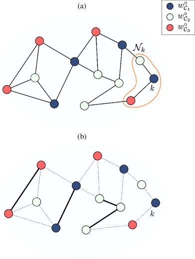
Figure 1: (Top) Example of a network topology involving three clusters, represented by three different colors. (Bottom) Clustered topology that will result for the network shown on top.

2.2 Topology Matrices

In preparation for the description of the proposed strategy, we introduce the $N\times N$ adjacency matrix $Y=[y_{\ell k}]$, whose elements are either zero or one depending on whether agents are linked by an edge or not. Specifically,

$${y}_{\ell k}=\begin{cases}1,&\ell\in\mathcal{N}_{k},\\ 0,&\textrm{otherwise}.\end{cases}$$ (3)

We assume that each agent $k$ belongs to its neighborhood set, $k\in{\cal N}_{k}$. The set ${\cal N}^{-}_{k}$ excludes $k$. Agents know their neighborhoods but they do not know which subset of their neighbors is subjected to data from the same model. In order to devise a procedure that allows agents to arrive at this information, we introduce a second $N\times N$ clustering matrix, denoted by $E_{i}$ at time $i$, in a manner similar to the adjacency matrix $Y$, except that the value at location $(\ell,k)$ will be set to one if agent $k$ believes at time $i$ that its neighbor $\ell$ belongs to the same cluster:

$${e}_{\ell k}(i)=\begin{cases}1,&\textrm{if }\ell\in{\cal N}_{k}\textrm{ and }k\textrm{ believes that }w_{k}^{\circ}=w_{\ell}^{\circ},\\ 0,&\textrm{otherwise}.\end{cases}$$ (4)

The entries of $E_{i}$ will be learned online. At every time $i$, we can then use these entries to infer which neighbors of $k$ are believed to belong to the same cluster as $k$; these would be the indices of the nonzero entries in the $k-$th column of $E_{i}$. We collect these indices into the neighborhood set, ${\cal N}_{k,i}$; this set is a subset of ${\cal N}_{k}$ and it evolves over time during the learning process. At any time $i$, agent $k$ will only be cooperating with the neighbors within ${\cal N}_{k,i}$. We will describe in the sequel how $E_{i}$ is learned.

2.3 Problem Formulation

We associate with each agent $k$ a strongly-convex and differentiable risk function $J_{k}(w_{k})$, with a unique minimum at $w_{k}^{\circ}$. In general, each risk $J_{k}(w_{k}):\mathbb{R}^{M}\rightarrow\mathbb{R}$, is defined as the expectation of some loss function ${Q}_{k}(\cdot)$, say,

$$J_{k}(w_{k})\;=\;\mathbb{E}\;{Q}_{k}(w_{k};\boldsymbol{z}_{k})$$ (5)

where $\boldsymbol{z}_{k}$ denotes random data sensed by agent $k$ and the expectation is over the distribution of this data. The network of agents is interested in estimating the minimizers of the following aggregate cost over the vectors $\{w_{k}\}$:

$$J^{\textrm{glob}}(w_{1},w_{2},\ldots,w_{N})\triangleq\sum_{k=1}^{N}J_{k}(w_{k}).$$ (6)

Since agents from different clusters do not share the same minimizers, the aggregate cost can be re-written as

$$J^{\textrm{glob}}(w_{{\cal C}_{1}},\ldots,w_{{\cal C}_{C}})\triangleq\sum_{m=1}^{C}\sum_{k\in{\cal C}_{m}}J_{k}(w_{k})$$ (7)

where $w_{k}^{\circ}=w_{{\cal C}_{m}}^{\circ}$. We collect the gradient vectors of the risk functions across the network into the aggregate vector

$$\nabla J({w})\triangleq\textrm{col}\{\nabla J_{1}({w}_{1}),\ldots,\nabla J_{N}({w}_{N})\}.$$ (8)

These gradients will not be available in most cases since the distribution of the data is not known to enable evaluation of the expectation of the loss functions. In stochastic-gradient implementations, it is customary to replace the above aggregate vector by the following approximation where the true gradients of the risk functions are replaced by

$$\widehat{\nabla J}({w})\triangleq\textrm{col}\{\widehat{\nabla J_{1}}({w}_{1}),\ldots,\widehat{\nabla J_{N}}({w}_{N})\}$$ (9)

where each $\widehat{\nabla J}_{k}(w_{k})$ is constructed from the gradient of the respective loss function

$$\widehat{\nabla J}_{k}(w_{k})\;=\;\nabla{Q}_{k}(w_{k};\boldsymbol{z}_{k})$$ (10)

evaluated at the corresponding data point, $\boldsymbol{z}_{k}$.

2.4 Assumptions

We list here the assumptions that are needed to drive the analysis. These assumptions are typical in the analysis of stochastic-gradient algorithms, and most of them are automatically satisfied by important cases of interest, such as when the risk functions are quadratic or logistic — see, e.g., [3, 20].

We thus assume that each individual cost function $J_{k}(w_{k})$ is twice-differentiable and $\tau_{k}-$strongly convex [3, 21, 22], for some $\tau_{k}>0$. We also require the gradient vector of $J_{k}(w_{k})$ to be $\zeta_{k}-$Lipschitz, i.e.,

$$\|\nabla J_{k}(w_{k_{1}})-\nabla J_{k}(w_{k_{2}})\|\leq\zeta_{k}\|w_{k_{1}}-w_{k_{2}}\|$$ (11)

for any $w_{k_{1}},w_{k_{2}}\in\mathbb{R}^{M}$. Thus, the Hessian matrix function $\nabla^{2}J_{k}(w_{k})$ is bounded by

$$\tau_{k}I_{M}\leq\nabla^{2}J_{k}(w_{k})\leq\ \zeta_{k}I_{M}$$ (12)

where $\tau_{k}\leq\zeta_{k}$. Each Hessian matrix function is also assumed to satisfy the Lipschitz condition:

$$\|\nabla^{2}J_{k}(w_{k_{1}})-\nabla^{2}J_{k}(w_{k_{2}})\|\leq\kappa_{k}\|w_{k_{1}}-w_{k_{2}}\|$$ (13)

for some $\kappa_{k}\geq 0$ and any $w_{k_{1}},w_{k_{2}}\in\mathbb{R}^{M}$. The network gradient noise is denoted by $\boldsymbol{s}_{i}(\boldsymbol{w}_{i-1})$ which is the random process defined by

$$\boldsymbol{s}_{i}(\boldsymbol{w}_{i-1})\triangleq\textrm{col}\{\boldsymbol{s}_{1,i}(\boldsymbol{w}_{1,i-1}),\ldots,\boldsymbol{s}_{N,i}(\boldsymbol{w}_{N,i-1})\}$$ (14)

where the gradient noise at agent $k$ at time $i$ is given by

$$\boldsymbol{s}_{k,i}(\boldsymbol{w}_{k,i-1})\triangleq\widehat{\nabla J}_{k}(\boldsymbol{w}_{k,i-1})-{\nabla J}_{k}(\boldsymbol{w}_{k,i-1}).$$ (15)

Here we are denoting the iterates $\boldsymbol{w}$ in boldface notation to indicate that they will actually be stochastic variables due to the approximation of the true gradients.

We let $\{\mathbb{F}_{k,i};i\geq 0\}$ denote the filtration that collects all information up to time $i$. We then denote the conditional covariance matrix of $\boldsymbol{s}_{k,i}(\boldsymbol{w}_{k,i-1})$ by

$${R}_{k,i}(\boldsymbol{w}_{k,i-1})\triangleq\mathbb{E}\left[\boldsymbol{s}_{k,i}(\boldsymbol{w}_{k,i-1})\boldsymbol{s}^{\intercal}_{k,i}(\boldsymbol{w}_{k,i-1})\mid\mathbb{F}_{k,i-1}\right].$$ (16)

It is assumed that the gradient noise process satisfies the following properties for any $\boldsymbol{w}_{k,i-1}$ in $\mathbb{F}_{k,i-1}$ [3]:

1. Martingale difference [3, 20]:

   $$\mathbb{E}\left[\boldsymbol{s}_{k,i}(\boldsymbol{w}_{k,i-1})\mid\mathbb{F}_{k,i-1}\right]=0$$ (17)

2. Bounded fourth-order moment [3, 20]:

   $$\mathbb{E}\left[\|\boldsymbol{s}_{k,i}(\boldsymbol{w}_{k,i-1})\|^{4}\mid\mathbb{F}_{k,i-1}\right]\leq\beta_{k}^{2}\|w_{k}^{\circ}-\boldsymbol{w}_{k,i-1}\|^{4}+\rho_{k}^{4}$$ (18)

   for some $\beta^{2}_{k},\rho^{4}_{k}\geq 0$.

3. Lipschitz conditional covariance function [3, 20]:

   $$\|{{R}}_{k,i}(w_{k}^{\circ})-{{R}}_{k,i}(\boldsymbol{w}_{k,i-1})\|\leq\theta_{k}\|w_{k}^{\circ}-\boldsymbol{w}_{k,i-1}\|^{\eta_{k}}$$ (19)

   for some $\theta_{k}\geq 0$ and $0<\eta_{k}\leq 4$.

4. Convergent conditional covariance matrix [3, 20]:

   $${R}_{k}\triangleq\lim_{i\rightarrow\infty}{{R}}_{k,i}(w_{k}^{\circ})>0$$ (20)

   where ${R}_{k}$ is symmetric and positive definite.

2.5 Data Model

We assume that each agent $k$ runs an independent stochastic gradient-descent algorithm of the form:

$$\boldsymbol{\psi}_{k,i}=\boldsymbol{\psi}_{k,i-1}-\mu_{k}\widehat{\nabla J_{k}}(\boldsymbol{\psi}_{k,i-1})$$ (21)

where $\mu_{k}>0$ is a small step-size parameter, and $\boldsymbol{\psi}_{k,i}$ denotes the intermediate estimate for $w^{\circ}_{k}$ at time $i$. Cooperation among agents will be limited to neighbors that belong to the same cluster. Therefore, following the update (21), ideally, agent $k$ should only share data with agent $\ell$ if ${w}^{\circ}_{k}={w}^{\circ}_{\ell}$. The agents do not know which agents in their neighborhood belong to the same cluster; this information is learned in real-time. Therefore, agent $k$ will only share data with agent $\ell$ if it believes that ${w}^{\circ}_{k}={w}^{\circ}_{\ell}$. Specifically, agent $k$ will combine the estimates from its neighbors in a convex manner as follows:

$$\boldsymbol{w}_{k,i}=\sum_{\ell=1}^{N}\boldsymbol{a}_{\ell k}(i)\boldsymbol{\psi}_{\ell,i}$$ (22)

where the nonnegative combination coefficients $\{\boldsymbol{a}_{\ell k}(i)\}$ satisfy

$$\boldsymbol{a}_{kk}(i)>0,\ \boldsymbol{a}_{\ell k}(i)=0\ \ \textrm{for}\ \ell\notin\boldsymbol{\mathcal{N}}_{k,i},\ \ \ \ \sum_{\ell=1}^{N}\boldsymbol{a}_{\ell k}(i)=1.$$ (23)

In the next section, we explain how the combination coefficients $\{\boldsymbol{a}_{\ell k}(i)\}$ are selected in order to perform the combined tasks of estimation and clustering.

3 Clustering Scheme

Let $\delta>0$ denote the smallest distance among the cluster models, $\{w^{\circ}_{{\cal C}_{m}}\}$. For any distinct $a,b\in\{1,\ldots,C\}$, it then holds that

$$\|w^{\circ}_{\mathcal{C}_{a}}-w^{\circ}_{\mathcal{C}_{b}}\|\geq\delta.$$ (24)

We introduce an $N\times N$ trust matrix $\boldsymbol{F}_{i}$; each entry $\boldsymbol{f}_{\ell k}(i)\in[0,1]$ of this matrix reflects the amount of trust that agent $k$ has in neighbor $\ell\in{\cal N}^{-}_{k}$ belonging to its cluster. The entries $\{\boldsymbol{f}_{\ell k}(i)\}$ are constructed as follows. Agent $k$ first computes the Boolean variable:

$$\boldsymbol{b}_{\ell k}(i)=\begin{cases}1,&\textrm{if }\|\boldsymbol{\psi}_{\ell,i}-\boldsymbol{w}_{k,i-1}\|^{2}\leq\alpha,\\ 0,&\textrm{otherwise}\end{cases}$$ (25)

where $\alpha$ is a threshold value. The trust level $\boldsymbol{f}_{\ell k}(i)$ is smoothed as follows:

$$\boldsymbol{f}_{\ell k}(i)=\nu\boldsymbol{f}_{\ell k}(i-1)+(1-\nu)\boldsymbol{b}_{\ell k}(i)$$ (26)

where the forgetting factor, $0<\nu<1$, determines the speed with which trust in neighbor $\ell$ accumulates over time. Once $\boldsymbol{f}_{\ell k}(i)$ exceeds some threshold $\gamma$, agent $k$ declares that neighbor $\ell$ belongs to its cluster and sets the corresponding entry $\boldsymbol{e}_{\ell k}(i)$ in matrix $\boldsymbol{E}_{i}$ to the value one:

$$\boldsymbol{e}_{\ell k}(i)=\begin{cases}1,\ \ \textrm{if }{\boldsymbol{f}_{\ell k}(i)\geq\gamma},\\ 0,\ \ \textrm{otherwise}\end{cases}$$ (27)

where $0<\gamma<1$. For completeness, we set for any agent $k$, $\boldsymbol{b}_{kk}(i)=\boldsymbol{f}_{kk}(i)=\boldsymbol{e}_{kk}(i)=1$. Observe that the computation of the binary variable $\boldsymbol{b}_{\ell k}(i)$ couples the $\boldsymbol{\psi}$ and $\boldsymbol{w}$ variables. Therefore, by using smoothed values $\{\boldsymbol{f}_{\ell k}(i)\}$ for the trust variables, we are able to couple the clustering and inference procedures into a single iterative algorithm rather than run them separately. The smoothing reduces the influence of erroneous clustering decisions on the inference task. The following listing summarizes the proposed strategy.

Initialize $\boldsymbol{F}_{-1}=\boldsymbol{B}_{-1}=\boldsymbol{E}_{-1}=I$ and $\boldsymbol{\psi}_{-1}=\boldsymbol{w}_{-1}=0$.

for $i\geq 0$ do

     for $k=1,\ldots,N$ do

$$\ \boldsymbol{\psi}_{k,i}=\boldsymbol{\psi}_{k,i-1}-\mu_{k}\widehat{\nabla J_{k}}(\boldsymbol{\psi}_{k,i-1})\$$ (28)

         for $\ell\in{\cal N}^{-}_{k}$ do

$$\boldsymbol{b}_{\ell k}(i)=\begin{cases}1,&\textrm{if }\|\boldsymbol{\psi}_{\ell,i}-\boldsymbol{w}_{k,i-1}\|^{2}\leq\alpha\\ 0,&\textrm{otherwise}\end{cases}$$ (29)

$$\boldsymbol{f}_{\ell k}(i)=\nu\boldsymbol{f}_{\ell k}(i-1)+(1-\nu)\;\boldsymbol{b}_{\ell k}(i)$$ (30)

               update $\boldsymbol{e}_{\ell k}(i)$ according to (27)

         end for

$$\textrm{select }\{\boldsymbol{a}_{\ell k}(i)\}\textrm{ according to}\leavevmode\nobreak\ (\ref{eq:matrix_a})\textrm{ and set \ \ \ }$$

$$\boldsymbol{w}_{k,i}=\displaystyle\sum_{\ell=1}^{N}\boldsymbol{a}_{\ell k}(i)\boldsymbol{\psi}_{\ell,i}$$ (31)

     end for

end for

Algorithm 1 (Distributed clustering scheme)

4 Mean-Square-Error Analysis

We now examine the mean-square performance of the proposed scheme.

We collect the estimates from across the network into the block vectors:

$$\boldsymbol{\psi}_{i} \triangleq\textrm{col}\{\boldsymbol{\psi}_{1,i},\boldsymbol{\psi}_{2,i},\ldots,\boldsymbol{\psi}_{N,i}\},$$ (32)

$$\boldsymbol{w}_{i} \triangleq\textrm{col}\{\boldsymbol{w}_{1,i},\boldsymbol{w}_{2,i},\ldots,\boldsymbol{w}_{N,i}\},$$ (33)

and define the matrices

$${\boldsymbol{{\cal A}}}_{i}\triangleq{\boldsymbol{{A}}}_{i}\otimes I_{M},\ \ \ {\cal M}\triangleq\textrm{diag}\{\mu_{1},\ldots,\mu_{N}\}\otimes I_{M}.$$ (34)

where $\boldsymbol{A}_{i}=[\boldsymbol{a}_{\ell k}(i)]$. From (21) we find that the network vector $\boldsymbol{\psi}_{i}$ evolves over time according to

$$\boldsymbol{\psi}_{i}=\boldsymbol{\psi}_{i-1}-{\cal M}\nabla J(\boldsymbol{\psi}_{i-1})-{\cal M}\boldsymbol{s}_{i}(\boldsymbol{\psi}_{i-1})$$ (35)

where $\nabla J(\cdot)$ and $\boldsymbol{s}_{i}(\cdot)$ are defined in (8) and (14). Likewise, from (22) we find that

$$\boldsymbol{w}_{i}={\boldsymbol{{\cal A}}}_{i}^{\intercal}\boldsymbol{\psi}_{i}.$$ (36)

To proceed, we introduce the error vectors

$$\widetilde{\boldsymbol{\psi}}_{k,i}\triangleq w_{k}^{\circ}-{\boldsymbol{\psi}}_{k,i},\ \ \ \widetilde{\boldsymbol{w}}_{k,i}\triangleq w_{k}^{\circ}-{\boldsymbol{w}}_{k,i},$$ (37)

and collect them from across the network into

$$\widetilde{\boldsymbol{\psi}}_{i} \triangleq\textrm{col}\{\widetilde{\boldsymbol{\psi}}_{1,i},\ldots,\widetilde{\boldsymbol{\psi}}_{N,i}\},$$ (38)

$$\widetilde{\boldsymbol{w}}_{i} \triangleq\textrm{col}\{\widetilde{\boldsymbol{w}}_{1,i},\ldots,\widetilde{\boldsymbol{w}}_{N,i}\}.$$ (39)

We further define the network mean-square deviation (MSD) before and after the fusion step at the time $i$ by

$$\textrm{MSD}_{{\psi}}(i) \triangleq\mathbb{E}\;\|{\widetilde{\boldsymbol{\psi}}}_{i}\|^{2},$$ (40)

$$\textrm{MSD}_{{w}}(i) \triangleq\mathbb{E}\;\|{\widetilde{\boldsymbol{w}}}_{i}\|^{2}.$$ (41)

4.1 Error Dynamics

Appealing to the mean-value theorem [3, p. 327] we can write

$$\nabla J(\boldsymbol{\psi}_{i-1})=-\boldsymbol{{\cal H}}_{i-1}\widetilde{\boldsymbol{\psi}}_{i-1}$$ (42)

where

$$\boldsymbol{{\cal H}}_{i-1}\triangleq\textrm{diag}\{\boldsymbol{H}_{k,i-1}\}_{k=1}^{N}$$ (43)

and each matrix $\boldsymbol{H}_{k,i-1}$ is given by

$$\boldsymbol{H}_{k,i-1}\triangleq\int_{0}^{1}\nabla^{2}J_{k}(w_{k}^{\circ}-t\widetilde{\boldsymbol{\psi}}_{k,i-1})dt.$$ (44)

Substituting (42) into (35) yields

$$\boldsymbol{\psi}_{i}=\boldsymbol{\psi}_{i-1}+{\cal M}\boldsymbol{{\cal H}}_{i-1}\widetilde{\boldsymbol{\psi}}_{i-1}-{\cal M}\boldsymbol{s}_{i}(\boldsymbol{\psi}_{i-1}).$$ (45)

By subtracting $w^{\circ}$ defined in (2) from both sides, we get

$$\widetilde{\boldsymbol{\psi}}_{i}=(I_{NM}-{\cal M}\boldsymbol{{\cal H}}_{i-1})\widetilde{\boldsymbol{\psi}}_{i-1}+{\cal M}\boldsymbol{s}_{i}(\boldsymbol{\psi}_{i-1})$$ (46)

which means that the error recursion for each individual agent $k$ is given by

$$\widetilde{\boldsymbol{\psi}}_{k,i}=(I_{M}-\mu_{k}\boldsymbol{H}_{k,i-1})\widetilde{\boldsymbol{\psi}}_{k,i-1}+\mu_{k}\boldsymbol{s}_{k,i}(\boldsymbol{\psi}_{k,i-1}).$$ (47)

It is argued in [3, p. 347] that for step-sizes $\mu_{k}$ satisfying

$$0<\mu_{k}<\frac{2\tau_{k}}{\zeta_{k}^{2}+\beta_{k}^{2}}$$ (48)

the mean-square-error quantity $\mathbb{E}\;\|\widetilde{\boldsymbol{\psi}}_{k,i}\|^{2}$ converges exponentially according to the recursion:

$$\mathbb{E}\;\|\widetilde{\boldsymbol{\psi}}_{k,i}\|^{2}\leq\xi_{k}\ \mathbb{E}\;\|\widetilde{\boldsymbol{\psi}}_{k,i-1}\|^{2}+\mu_{k}^{2}\rho_{k}^{2}$$ (49)

where $0\leq\xi_{k}<1$ and is given by

$$\xi_{k}=1-2\mu_{k}\tau_{k}+\mu_{k}^{2}(\zeta_{k}^{2}+\beta_{k}^{2}).$$ (50)

It is further shown in [3, pp. 352, 378] that for small step-sizes satisfying (48), the error recursion (46) has bounded first, second, and fourth-order moments in the following sense:

$$\limsup_{i\rightarrow\infty}\;\|\mathbb{E}\;\widetilde{\boldsymbol{\psi}}_{i}\|={\cal O}(\mu_{\max})$$ (51)

$$\limsup_{i\rightarrow\infty}\;\mathbb{E}\;\|\widetilde{\boldsymbol{\psi}}_{i}\|^{2}={\cal O}(\mu_{\max})$$ (52)

$$\limsup_{i\rightarrow\infty}\;\mathbb{E}\;\|\widetilde{\boldsymbol{\psi}}_{i}\|^{4}={\cal O}(\mu_{\max}^{2})$$ (53)

where $\mu_{\max}$ is the maximum step-size across all agents.

We further introduce the constant block diagonal matrix:

$${\cal H}\triangleq\textrm{diag}\{H_{1},\ldots,H_{N}\},\ \ \ {H_{k}}\triangleq\nabla^{2}J_{k}(w_{k}^{\circ}),$$ (54)

and replace (46) by the approximate recursion

$$\widetilde{\boldsymbol{\psi}}^{\prime}_{i}=(I_{NM}-{\cal M}{{\cal H}})\widetilde{\boldsymbol{\psi}}^{\prime}_{i-1}+{\cal M}\boldsymbol{s}_{i}(\boldsymbol{\psi}_{i-1})$$ (55)

where the random matrix $\boldsymbol{\cal H}_{i-1}$ is replaced by ${\cal H}$. It was also shown in [3, pp. 382, 384] that, for sufficiently small step-sizes, the error iterates that are generated by this recursion satisfy:

$$\lim_{i\rightarrow\infty}\ \mathbb{E}\;\widetilde{\boldsymbol{\psi}}^{\prime}_{i}=0$$ (56)

$$\limsup_{i\rightarrow\infty}\;\mathbb{E}\;\|\widetilde{\boldsymbol{\psi}}^{\prime}_{i}\|^{2}={\cal O}(\mu_{\max})$$ (57)

$$\limsup_{i\rightarrow\infty}\;\mathbb{E}\;\|\widetilde{\boldsymbol{\psi}}_{i}-\widetilde{\boldsymbol{\psi}}^{\prime}_{i}\|^{2}={\cal O}(\mu_{\max}^{2})$$ (58)

$$\limsup_{i\rightarrow\infty}\;\mathbb{E}\;\|\widetilde{\boldsymbol{\psi}}^{\prime}_{i}\|^{2}=\limsup_{i\rightarrow\infty}\;\mathbb{E}\;\|\widetilde{\boldsymbol{\psi}}_{i}\|^{2}+{\cal O}(\mu_{\max}^{3/2}).$$ (59)

These results imply that, for large enough $i$, the errors $\widetilde{\boldsymbol{\psi}}$ and $\widetilde{\boldsymbol{\psi}}^{\prime}$ are close to each other in the mean-square-error sense.

4.2 One Useful Property

The above construction guarantees one useful property if the clustering process does not incur errors of type II, meaning that links that should be disconnected are indeed disconnected. This implies that $w_{\ell}^{\circ}=w_{k}^{\circ}$ whenever $\boldsymbol{a}_{\ell k}(i)>0$. Using (23), it follows that

$$\sum_{\ell=1}^{N}\boldsymbol{a}_{\ell k}(i)w^{\circ}_{\ell}=w^{\circ}_{k}$$ (60)

or, equivalently,

$${\boldsymbol{\cal A}}^{\intercal}_{i}w^{\circ}=w^{\circ}.$$ (61)

Subtracting $w^{\circ}$ from both sides of (36) yields,

$$w^{\circ}-{\boldsymbol{w}}_{i}=w^{\circ}-{\boldsymbol{\cal A}}^{\intercal}_{i}{{\boldsymbol{\psi}}}_{i}.$$ (62)

Using (61) we rewrite (62) as:

$$\widetilde{\boldsymbol{w}}_{i}={\boldsymbol{\cal A}}^{\intercal}_{i}{\widetilde{\boldsymbol{\psi}}}_{i}.$$ (63)

Taking the block maximum norm [23, p. 435] of both sides and using the sub-multiplicative property of norms implies that

$$\|\widetilde{\boldsymbol{w}}_{i}\|_{b,\infty}\leq\|{\boldsymbol{\cal A}}^{\intercal}_{i}\|_{b,\infty}\ \|{\widetilde{\boldsymbol{\psi}}}_{i}\|_{b,\infty}=\|{\widetilde{\boldsymbol{\psi}}}_{i}\|_{b,\infty}$$ (64)

since $\boldsymbol{A}_{i}$ is left-stochastic and, therefore, $\|\boldsymbol{\cal A}_{i}^{\intercal}\|_{b,\infty}=1$. It follows that

$$\mathbb{E}\;\|{\widetilde{\boldsymbol{w}}}_{i}\|_{b,\infty}\leq\mathbb{E}\;\|{\widetilde{\boldsymbol{\psi}}}_{i}\|_{b,\infty}.$$ (65)

Results (64) and (65) ensure that the size of the error in the $w$ domain is bounded by the size of the error in the $\psi$ domain if there are no errors of type II during clustering.

5 Performance Analysis

We are ready to examine the behavior of the probabilities of erroneous decisions of types I and II for each agent $k$, namely, the probabilities that a link between $k$ and one of its neighbors will be either erroneously disconnected (when it should be connected) or erroneously connected (when it should be disconnected):

$$\textrm{Type-I: }w_{\ell}^{\circ}=w_{k}^{\circ} \textrm{ and }\boldsymbol{a}_{\ell k}(i)=0,$$ (66)

$$\textrm{Type-II: }w_{\ell}^{\circ}\neq w_{k}^{\circ} \textrm{ and }\boldsymbol{a}_{\ell k}(i)\neq 0$$ (67)

for any $\ell\in{\cal N}_{k}$. After long enough $i$, these probabilities are denoted respectively by:

$$P_{\textrm{I}} =\Pr\ (\boldsymbol{f}_{\ell k}(i)<\gamma\ |\ w_{\ell}^{\circ}=w_{k}^{\circ}),$$ (68)

$$P_{\textrm{II}} =\Pr\ (\boldsymbol{f}_{\ell k}(i)\geq\gamma\ |\ w_{\ell}^{\circ}\neq w_{k}^{\circ}).$$ (69)

Assessing the probabilities (68) and (69) is a challenging task and needs to be pursued under some simplifying conditions to facilitate the analysis. This is due to the stochastic nature of the clustering and learning processes, and due to the coupling among the agents. Our purpose is to provide insights into the performance of these processes after sufficient learning time has elapsed. The analysis that follows adjusts the approach of [14] to the current setting. Different from [14] where there were only two models and all agents were trying to converge to one of these two models, we now have a multitude of clusters and agents that are trying to converge to their own cluster model.

5.1 Smoothing Process

In order to determine bounds for $P_{\textrm{I}}$ and $P_{\textrm{II}}$ we study the probability distribution of the trust variable $\boldsymbol{f}_{\ell k}(i)$. We have from (26) that:

$$\boldsymbol{f}_{\ell k}(i)=\nu^{i+1}\boldsymbol{f}_{\ell k}(-1)+(1-\nu)\sum_{j=0}^{i}\nu^{j}\boldsymbol{b}_{\ell k}(i-j)$$ (70)

where $\boldsymbol{b}_{\ell k}(i)$ is modelled as a Bernoulli random variable with success probability $p$:

$$\boldsymbol{b}_{\ell k}(i)=\begin{cases}1,\textrm{with probability }p,\\ 0,\textrm{with probability }(1-p).\end{cases}$$ (71)

We already know from (49) that, after sufficient time, the iterates $\boldsymbol{\psi}_{k,i}$ converge to the true models $w_{k}^{\circ}$ in the mean-square-error sense. Hence, it is reasonable to assume that the value of $p$ becomes largely time-invariant and corresponds to the probability of the event described by

$$\|\boldsymbol{\psi}_{\ell,i}-\boldsymbol{w}_{k,i-1}\|^{2}\leq\alpha,\textrm{ for large }i.$$ (72)

We denote the probabilities of true and false assignments by

$$P_{d}=\Pr\ (\boldsymbol{b}_{\ell k}(i)=1\ |\ w_{\ell}^{\circ}=w_{k}^{\circ}),$$ (73)

$$P_{f}=\Pr\ (\boldsymbol{b}_{\ell k}(i)=1\ |\ w_{\ell}^{\circ}\neq w_{k}^{\circ}).$$ (74)

These probabilities also satisfy:

$$(1-P_{d}) =\Pr\ (\|\boldsymbol{\psi}_{\ell,i}-\boldsymbol{w}_{k,i-1}\|^{2}>\alpha\ |\ w^{\circ}_{\ell}=w^{\circ}_{k}),$$ (75)

$$P_{f} =\Pr\ (\|\boldsymbol{\psi}_{\ell,i}-\boldsymbol{w}_{k,i-1}\|^{2}\leq\alpha\ |\ w^{\circ}_{\ell}\neq w^{\circ}_{k}).$$ (76)

After sufficient iterations, the influence of the initial condition in (70) can be ignored and we can approximate $\boldsymbol{f}_{\ell k}(i)$ by the following random geometric series:

$$\boldsymbol{f}_{\ell k}(i)\approx(1-\nu)\sum_{j=0}^{i}\nu^{j}\boldsymbol{b}_{\ell k}(i-j).$$ (77)

As explained in [14], although it is generally not true, we can simplify the analysis by assuming that, for large enough $i$, the random variables $\{\boldsymbol{b}_{\ell k}(m)\}$ in (77) are independent and identically distributed. This assumption is motivated by the fact that the models observed by the different clusters are assumed to be sufficiently distinct from each other by virtue of (24).

Now, recall that Markov’s inequality [24, p. 47] implies that for any nonnegative random variable $\boldsymbol{x}$ and positive scalar $u$, it holds that:

$$\Pr\ (\boldsymbol{x}\geq u)=\Pr\ (\boldsymbol{x}^{2}\geq u^{2})\leq\frac{\mathbb{E}\;\boldsymbol{x}^{2}}{u^{2}}.$$ (78)

To apply (78) to the variable $\boldsymbol{f}_{\ell k}(i)$, we need to determine its second-order moment. For this purpose, we follow [14] and introduce the change of variable:

$$\boldsymbol{b}^{\circ}_{\ell k}(i-j)\triangleq\frac{\boldsymbol{b}_{\ell k}(i-j)-p}{\sqrt{p(1-p)}}.$$ (79)

It can be verified that the variables {$\boldsymbol{b}^{\circ}_{\ell k}(m)$} are i.i.d. with zero mean and unit variance. As a result, we rewrite (77) for large $i$ as:

$$\boldsymbol{f}_{\ell k}(i)\approx p+\sqrt{p(1-p)}\boldsymbol{f}^{\circ}_{\ell k}(i)$$ (80)

where

$$\boldsymbol{f}^{\circ}_{\ell k}(i)\triangleq(1-\nu)\sum_{j=0}^{i}\nu^{j}\boldsymbol{b}^{\circ}_{\ell k}(i-j)$$ (81)

has zero mean and its variance is given by

$$\textrm{Var}\ [{\boldsymbol{f}^{\circ}_{\ell k}}(i)] =\mathbb{E}\;\big{[}{\boldsymbol{f}^{\circ}_{\ell k}}(i)\big{]}^{2}-\Big{[}\mathbb{E}\;{\boldsymbol{f}^{\circ}_{\ell k}}(i)\Big{]}^{2}$$

$$=\frac{1-\nu}{1+\nu}(1-\nu^{2(i+1)})\approx\frac{1-\nu}{1+\nu}.$$ (82)

Returning to (68) we now have, with $p$ replaced by $P_{d}$:

$$P_{\textrm{I}} \approx\textrm{Pr}\ (\boldsymbol{f}_{\ell k}(i)<\gamma\ |\ w_{\ell}^{\circ}=w_{k}^{\circ})$$

$$\leq\Pr\ \bigg{(}|\boldsymbol{f}^{\circ}_{\ell k}(i)|>\frac{P_{d}-\gamma}{\sqrt{P_{d}(1-P_{d})}}\ \bigg{|}\ w_{\ell}^{\circ}=w_{k}^{\circ}\bigg{)}$$

$$\leq\frac{1-\nu}{1+\nu}\cdot\frac{P_{d}(1-P_{d})}{(P_{d}-\gamma)^{2}}$$ (83)

where we applied (78) and the fact that, for any two generic events $B_{1}$ and $B_{2}$, if $B_{1}$ implies $B_{2}$, then the probability of event $B_{1}$ is less than the probability of event $B_{2}$ [25]. Similarly, by replacing $p$ by $P_{f}$, we obtain

$$P_{\textrm{II}}\leq\frac{1-\nu}{1+\nu}\cdot\frac{P_{f}(1-P_{f})}{(\gamma-P_{f})^{2}}.$$ (84)

In expressions (83) and (84), it is assumed that the size of the threshold value $\gamma$ used in (27) satisfies $\gamma<P_{d}$ and $\gamma>P_{f}$. Since we usually desire the probability of false alarm to be small and the probability of detection to be close to one, these conditions can be met by $\gamma\in(0,1)$. We show in the next section that this is indeed the case.

Results (83) and (84) provide bounds on the probabilities of errors I and II. We next establish that $P_{d}\rightarrow 1$ and $P_{f}\rightarrow 0$ to conclude that $P_{\textrm{I}}\rightarrow 0$ and $P_{\textrm{II}}\rightarrow 0$.

5.2 The Distribution of the Variables

After sufficient iterations and for small enough step-sizes, it is known that each $\boldsymbol{\psi}_{\ell,i}$ exhibits a distribution that is nearly Gaussian [26, 27, 28, 29, 30, 31]:

$$\boldsymbol{\psi}_{\ell,i}\sim\mathbb{N}\;(w_{\ell}^{\circ},\mu_{\ell}\Gamma_{\ell})$$ (85)

where the matrix $\Gamma_{\ell}$ is symmetric, positive semi-definite, and the solution to the following Lyapunov equation [26]:

$$H_{\ell}\Gamma_{\ell}+\Gamma_{\ell}H_{\ell}=R_{\ell}$$ (86)

where the Hessian matrix $H_{\ell}$ is defined by (54) and $R_{\ell}$ is the steady-state covariance matrix of the gradient noise at agent $\ell$ defined by (20). We next introduce the vector

$$\boldsymbol{\bar{w}}_{k,i}^{\circ}\triangleq\sum_{\ell=1}^{N}{\boldsymbol{a}}_{\ell k}(i)w^{\circ}_{\ell}.$$ (87)

which should be compared with expression (22). The vector (87) is the result of fusing the actual models using the same combination weights available at time $i$. It follows that $\boldsymbol{w}_{k,i}$ exhibits a distribution that is nearly Gaussian since the iterates $\{\boldsymbol{\psi}_{\ell,i}\}$ can be assumed to be independent of each other due to the decoupled nature of their updates:

$$\boldsymbol{w}_{k,i}\sim\mathbb{N}\;(\boldsymbol{\bar{w}}^{\circ}_{k,i},\boldsymbol{\Omega}_{k,i})$$ (88)

where $\boldsymbol{\Omega}_{k,i}$ is symmetric, positive semi-definite, and given by

$$\boldsymbol{\Omega}_{k,i}\triangleq\sum_{\ell=1}^{N}\mu_{\ell}\;{\boldsymbol{a}}^{2}_{\ell k}(i){\Gamma}_{\ell}.$$ (89)

Let

$$\boldsymbol{g}_{\ell k,i}\triangleq\boldsymbol{\psi}_{\ell,i}-\boldsymbol{w}_{k,i-1}$$ (90)

and note that $\boldsymbol{g}_{\ell k,i}$ is again approximately Gaussian distributed with

$$\boldsymbol{g}_{\ell k,i}\sim\mathbb{N}\ (\boldsymbol{\bar{g}}_{i},\boldsymbol{\Delta}_{\ell k,i})$$ (91)

where

$$\boldsymbol{\bar{g}}_{i}\triangleq w^{\circ}_{\ell}-\boldsymbol{\bar{w}}^{\circ}_{k,i-1}$$ (92)

and $\boldsymbol{\Delta}_{\ell k,i}$ is symmetric, positive semi-definite, and bounded by (in view of Jensen’s inequality[3, p. 769]):

$$\boldsymbol{\Delta}_{\ell k,i}\leq 2\;\big{(}\;\mu_{\ell}{\Gamma}_{\ell}+\boldsymbol{\Omega}_{k,i-1}\;\big{)}.$$ (93)

From (89), (93) and for any $\ell$ and $k$ it holds that:

$$\boldsymbol{\Delta}_{\ell k,i}={\cal O}(\mu_{\max}).$$ (94)

5.3 The Statistics of $\|\boldsymbol{g}_{\ell k,i}\|^{2}$

We now examine the statistics of the main test variable for our algorithm from (25), namely, $\|\boldsymbol{g}_{\ell k,i}\|^{2}$. Let $\{\mathbb{A}_{k,i-1};i>0\}$ denote the filtration that collects all $\{\boldsymbol{a}_{\ell k}(i-1)\}$ information up to time $i-1$. Then, note that

$$\mathbb{E}\;\left[\|\boldsymbol{g}_{\ell k,i}\|^{2}|\;\mathbb{A}_{k,i-1}\right] =\mathbb{E}\;\left[\textrm{Tr}\;\big{(}\boldsymbol{g}_{\ell k,i}\boldsymbol{g}_{\ell k,i}^{\intercal}\big{)}\big{|}\;\mathbb{A}_{k,i-1}\right]$$

$$=\|\boldsymbol{\bar{g}}_{i}\|^{2}+\textrm{Tr}\;(\boldsymbol{\Delta}_{\ell k,i}).$$ (95)

Since $\boldsymbol{g}_{\ell k,i}$ is Gaussian, it holds that

$$\mathbb{E}\; \left[\|\boldsymbol{g}_{\ell k,i}\|^{4}|\;\mathbb{A}_{k,i-1}\right]$$

$$=\mathbb{E}\;\left[\|\boldsymbol{g}_{\ell k,i}-\boldsymbol{\bar{g}}_{i}+\boldsymbol{\bar{g}}_{i}\|^{4}|\;\mathbb{A}_{k,i-1}\right]$$

$$=\mathbb{E}\;\left[\big{(}\ \|\boldsymbol{g}_{\ell k,i}-\boldsymbol{\bar{g}}_{i}\|^{2}+2(\boldsymbol{g}_{\ell k,i}-\boldsymbol{\bar{g}}_{i})^{\intercal}\boldsymbol{\bar{g}}_{i}+\|\boldsymbol{\bar{g}}_{i}\|^{2}\big{)}^{2}\big{|}\;\mathbb{A}_{k,i-1}\right]$$

$$=\mathbb{E}\;\left[\|\boldsymbol{g}_{\ell k,i}-\boldsymbol{\bar{g}}_{i}\|^{4}|\;\mathbb{A}_{k,i-1}\right]$$

$$+2\mathbb{E}\left[\;\|\boldsymbol{g}_{\ell k,i}-\boldsymbol{\bar{g}}_{i}\|^{2}\|\boldsymbol{\bar{g}}_{i}\|^{2}|\;\mathbb{A}_{k,i-1}\right]+\|\boldsymbol{\bar{g}}_{i}\|^{4}$$

$$+4\boldsymbol{\bar{g}}_{i}^{\intercal}\mathbb{E}\;\big{[}\ (\boldsymbol{g}_{\ell k,i}-\boldsymbol{\bar{g}}_{i})(\boldsymbol{g}_{\ell k,i}-\boldsymbol{\bar{g}}_{i})^{\intercal}|\;\mathbb{A}_{k,i-1}\big{]}\boldsymbol{\bar{g}}_{i}$$

$$=\mathbb{E}\;\left[\|\boldsymbol{g}_{\ell k,i}-\boldsymbol{\bar{g}}_{i}\|^{4}|\;\mathbb{A}_{k,i-1}\right]+2\;\textrm{Tr}\;(\boldsymbol{\Delta}_{\ell k,i})\|\boldsymbol{\bar{g}}_{i}\|^{2}$$

$$\ +\|\boldsymbol{\bar{g}}_{i}\|^{4}+4\|\boldsymbol{\bar{g}}_{i}\|^{2}_{\boldsymbol{\Delta}_{\ell k,i}}$$ (96)

where all odd order moments of $(\boldsymbol{g}_{\ell k,i}-\boldsymbol{\bar{g}}_{i})$ are zero. Likewise,

$$\big{(}\mathbb{E}\; \left[\|\boldsymbol{g}_{\ell k,i}\|^{2}|\;\mathbb{A}_{k,i-1}\right]\big{)}^{2}$$

$$=\big{(}\mathbb{E}\;\left[\|\boldsymbol{g}_{\ell k,i}-\boldsymbol{\bar{g}}_{i}+\boldsymbol{\bar{g}}_{i}\|^{2}|\;\mathbb{A}_{k,i-1}\right]\big{)}^{2}$$

$$=\big{(}\mathbb{E}\;\left[\|\boldsymbol{g}_{\ell k,i}-\boldsymbol{\bar{g}}_{i}\|^{2}|\;\mathbb{A}_{k,i-1}\right]+\|\boldsymbol{\bar{g}}_{i}\|^{2}\big{)}^{2}$$

$$=[\;\textrm{Tr}\;(\boldsymbol{\Delta}_{\ell k,i})\;]^{2}+2\;\textrm{Tr}\;(\boldsymbol{\Delta}_{\ell k,i})\|\boldsymbol{\bar{g}}_{i}\|^{2}$$

$$\ +\|\boldsymbol{\bar{g}}_{i}\|^{4}.$$ (97)

According to Lemma A.2 of [32, p. 11], we have

$$\mathbb{E}\; \left[\|\boldsymbol{g}_{\ell k,i}-\boldsymbol{\bar{g}}_{i}\|^{4}|\;\mathbb{A}_{k,i-1}\right]$$

$$=[\;\textrm{Tr}\;(\boldsymbol{\Delta}_{\ell k,i})\;]^{2}+2\;\textrm{Tr}\;(\boldsymbol{\Delta}_{\ell k,i}^{2}).$$ (98)

Using (5.3) and (5.3), the variance of $\|\boldsymbol{g}_{\ell k,i}\|^{2}$ is given by

Var $$\left[\|\boldsymbol{g}_{\ell k,i}\|^{2}|\;\mathbb{A}_{k,i-1}\right]$$

$$=4\|\boldsymbol{\bar{g}}_{i}\|_{\boldsymbol{\Delta}_{\ell k,i}}^{2}+2\;\textrm{Tr}\;(\boldsymbol{\Delta}_{\ell k,i}^{2}).$$ (99)

Note from (5.3) that the mean of $\|\boldsymbol{g}_{\ell k,i}\|^{2}$ is dominated by $\|\boldsymbol{\bar{g}}_{i}\|^{2}$ for sufficiently small step-sizes. It follows from the Chebyshev’s inequality [33, p. 455] that:

$$\Pr\; \bigg{(}\big{|}\|\boldsymbol{g}_{\ell k,i}\|^{2}-\mathbb{E}\;\left[\|\boldsymbol{g}_{\ell k,i}\|^{2}|\;\mathbb{A}_{k,i-1}\right]\big{|}\geq u\bigg{|}\;\mathbb{A}_{k,i-1}\bigg{)}$$

$$\leq\frac{\textrm{Var}\;\left[\|\boldsymbol{g}_{\ell k,i}\|^{2}|\;\mathbb{A}_{k,i-1}\right]}{u^{2}}={\cal O}(\mu_{\max})$$ (100)

for any constant $u>0$, which implies that the variance of $\|\boldsymbol{g}_{\ell k,i}\|^{2}$ is in the order of $\mu_{\max}$. Therefore, when $w_{\ell}^{\circ}=w_{k}^{\circ}$ the probability mass of $\|\boldsymbol{g}_{\ell k,i}\|^{2}$ will concentrate around $\mathbb{E}(\|\boldsymbol{g}_{\ell k,i}\|^{2})$, which is in the order of ${\cal O}(\mu_{\max})\approx 0$. On the other hand, when $w_{\ell}^{\circ}\neq w_{k}^{\circ}$, the probability mass of $\|\boldsymbol{g}_{\ell k,i}\|^{2}$ will concentrate around $\mathbb{E}(\|\boldsymbol{g}_{\ell k,i}\|^{2})\approx\|\boldsymbol{\bar{g}}_{i}\|^{2}>0$. Obviously the threshold should be chosen as: $0<\alpha<\delta^{2}$, where $\delta$ is the clustering resolution.

5.4 Error Probabilities

It is seen from (75) and (76) that $1-P_{d}$ corresponds to the right tail probability of $\|\boldsymbol{g}_{\ell k,i}\|^{2}$ when $w^{\circ}_{\ell}=w^{\circ}_{k}$, and $P_{f}$ corresponds to the left tail probability of $\|\boldsymbol{g}_{\ell k,i}\|^{2}$ when $w^{\circ}_{\ell}\neq w^{\circ}_{k}$. To examine these probabilities, we follow arguments similar to [20] and apply them to the current context. We introduce the eigen-decomposition

$$\boldsymbol{\Delta}_{\ell k,i}=\boldsymbol{U}_{i}\boldsymbol{\Lambda}_{i}\boldsymbol{U}_{i}^{\intercal}$$ (101)

where $\boldsymbol{U}_{i}$ is orthonormal and $\boldsymbol{\Lambda}_{i}$ is diagonal and nonnegative-definite. We further introduce the normalized variables:

$$\boldsymbol{x}_{i} \triangleq\boldsymbol{\Lambda}_{i}^{-1/2}\boldsymbol{U}_{i}^{\intercal}\boldsymbol{g}_{\ell k,i},$$ (102)

$$\boldsymbol{\bar{x}}_{i} \triangleq\boldsymbol{\Lambda}_{i}^{-1/2}\boldsymbol{U}_{i}^{\intercal}\boldsymbol{\bar{g}}_{i}$$ (103)

and it follows from (91), (102), and (103) that

$$\boldsymbol{x}_{i}\sim\mathbb{N}\ (\boldsymbol{\bar{x}}_{i},\mathds{I}_{M}).$$ (104)

Note also from (102) that

$$\|\boldsymbol{g}_{\ell k,i}\|^{2}=\boldsymbol{x}_{i}^{\intercal}\boldsymbol{\Lambda}_{i}\boldsymbol{x}_{i}=\sum_{h=1}^{M}\boldsymbol{\lambda}_{h,i}\boldsymbol{x}_{h,i}^{2}.$$ (105)

where $\boldsymbol{x}_{h,i}$ denotes the $h-$th element of $\boldsymbol{x}_{i}$ and $\boldsymbol{\lambda}_{h,i}$ denotes the $h-$th diagonal element of $\boldsymbol{\Lambda}_{i}$.

5.4.1 The probability $1-P_{d}$

It follows from the inequality

$$\|\boldsymbol{g}_{\ell k,i}\|^{2}=\boldsymbol{x}_{i}^{\intercal}\boldsymbol{\Lambda}_{i}\boldsymbol{x}_{i}\leq\|\boldsymbol{\Delta}_{\ell k,i}\|\cdot\|\boldsymbol{x}_{i}\|^{2},$$ (106)

that the following relation is satisfied

$$\{\|\boldsymbol{g}_{\ell k,i}\|^{2}>\alpha\}\subseteq\{\|\boldsymbol{\Delta}_{\ell k,i}\|\cdot\|\boldsymbol{x}_{i}\|^{2}>\alpha\}.$$ (107)

Defining

$$\boldsymbol{\alpha}_{k}(i)\triangleq\alpha/\|\boldsymbol{\Delta}_{\ell k,i}\|$$ (108)

, we can write using (107):

$$\Pr\ (\|\boldsymbol{g}_{\ell k,i}\|^{2}>\alpha\ |\ w^{\circ}_{\ell}=w^{\circ}_{k})\leq\Pr\ (\|\boldsymbol{x}_{i}\|^{2}>\boldsymbol{\alpha}_{k}(i)\ |\ \boldsymbol{\bar{x}}_{i}=0).$$ (109)

We know from (104) that

$$\|\boldsymbol{x}_{i}\|^{2}\sim{\cal X}_{M}^{2}$$ (110)

where ${\cal X}_{M}^{2}$ denotes the Chi-square distribution with $M$ degrees of freedom and its mean value is $M$. According to the Chernoff bound for the central Chi-square distribution with $M$ degrees of freedom we have

$$\Pr\; \big{(}\;\|\boldsymbol{x}_{i}\|^{2}>\boldsymbol{\alpha}_{k}(i)\;\big{|}\;\boldsymbol{\bar{x}}_{i}=0\;\big{)}$$

$$=\Pr\;\bigg{(}\|\boldsymbol{x}_{i}\|^{2}>\frac{M\cdot\boldsymbol{\alpha}_{k}(i)}{M}\ \bigg{|}\ \boldsymbol{\bar{x}}_{i}=0\bigg{)}$$

$$\leq\textrm{exp}\Big{[}-\frac{M}{2}\Big{(}\frac{\boldsymbol{\alpha}_{k}(i)}{M}-\textrm{log}\;\Big{(}1+\frac{\boldsymbol{\alpha}_{k}(i)}{M}-1\Big{)}\Big{)}\Big{]}$$

$$=\Big{(}\frac{\boldsymbol{\alpha}_{k}(i)\cdot e}{M}\Big{)}^{M/2}\cdot\textrm{exp}\Big{[}-\frac{\boldsymbol{\alpha}_{k}(i)}{2}\ \Big{]}$$ (111)

where $e$ is Euler’s number. For small enough step-sizes we conclude from (94), (108), and (5.4.1) that after sufficient iterations, it holds that:

$$(1-{P}_{d})\leq{\cal O}(e^{-c_{1}/\mu_{\max}})$$ (112)

for some constant $c_{1}>0$.

5.4.2 The probability $P_{f}$

The approximate characteristic function of $\|\boldsymbol{g}_{\ell k,i}\|^{2}$ [20, Eq. (118)] when $w^{\circ}_{\ell}\neq w^{\circ}_{k}$ is given by:

$$c_{\|\boldsymbol{g}_{\ell k,i}\|^{2}}(t)\approx e^{jt\|w^{\circ}_{\ell}-w^{\circ}_{k}\|^{2}-2t^{2}\|w^{\circ}_{\ell}-w^{\circ}_{k}\|^{2}_{\boldsymbol{\Lambda_{i}}}}$$ (113)

which implies that for sufficiently small $\mu_{\max}$,

$$\|\boldsymbol{g}_{\ell k,i}\|^{2}\sim\mathbb{N}\;(\|w^{\circ}_{\ell}-w^{\circ}_{k}\|^{2},4\|w^{\circ}_{\ell}-w^{\circ}_{k}\|^{2}_{\boldsymbol{\Lambda_{i}}}).$$ (114)

Therefore, from [20] we obtain that

$$\Pr \ (\|\boldsymbol{g}_{\ell k,i}\|^{2}<\alpha\ |w^{\circ}_{\ell}\neq w^{\circ}_{k}\ )\approx{Q}\bigg{(}\frac{\|w^{\circ}_{\ell}-w^{\circ}_{k}\|^{2}-\alpha}{2\|w^{\circ}_{\ell}-w^{\circ}_{k}\|_{\boldsymbol{\Lambda_{i}}}}\bigg{)}$$

$$\leq\frac{1}{2}\;\textrm{exp}\;\bigg{[}-\frac{(\|w^{\circ}_{\ell}-w^{\circ}_{k}\|^{2}-\alpha)^{2}}{8\|w^{\circ}_{\ell}-w^{\circ}_{k}\|^{2}_{\boldsymbol{\Lambda_{i}}}}\bigg{]}$$ (115)

where the letter $Q$ refers here to the traditional $Q-$function (the tail probability of the standard Gaussian distribution). For small enough step-sizes, after sufficient iterations and from (94), (101), and (5.4.2), it holds that

$${P}_{f} \leq{\cal O}(e^{-c_{2}/\mu_{\max}})$$ (116)

for some constant $c_{2}>0$. It is then seen that the probabilities $P_{\textrm{I}}$ and $P_{\textrm{II}}$ are expected to approach zero exponentially fast for vanishing step-sizes.

6 Linking Application

6.1 Clustering With Linking Scheme

We propose in this section an additional mechanism to enhance the performance of each cluster by using the unused links to relay information. Figure 2 shows the linked topology that results for the same example shown earlier in Fig. 1(b). The figure shows that the links which are supposed to be unused for sharing data among neighbors belonging to different clusters, are used now to relay data among agents.

We assume in this section that the links among agents are symmetric, i.e. if $\ell\in{\cal N}_{k}\Longleftrightarrow k\in{\cal N}_{\ell}$. Under normal operation, each agent $k$ will be receiving and processing iterates only from those neighbors that it believes belong to the same cluster as $k$.

We modify this operation by allowing $k$ to receive iterates from all of its neighbors. It will continue to use the iterates from neighbors in the same cluster to update its weight estimate $\boldsymbol{w}_{k,i}$. The iterates that arrive from neighbors that may belong to other clusters are not used during this fusion process. Instead, they will be relayed forward by agent $k$ as follows. For each of its neighbors $\ell\in{\cal N}_{k}$, agent $k$ will send $\boldsymbol{\psi}_{k,i}$ and another vector $\boldsymbol{\phi}_{k\ell,i}$ The vector $\boldsymbol{\phi}_{k\ell,i}$ is constructed as follows. Agent $k$ chooses from among all the iterates it receives from its neighbors, that iterate that is closest to $\boldsymbol{\psi}_{\ell,i}$:

$$\boldsymbol{\phi}_{k\ell,i}\;=\ \;\underset{\begin{subarray}{c}\{k,m\}\\ \forall m\in{\cal N}_{k},\;m\notin{\cal N}_{\ell}\end{subarray}}{\mbox{{a}rg min}\ \ \|\boldsymbol{\psi}_{m,i}-\boldsymbol{\psi}_{\ell,i}\|^{2}.}$$ (117)

Observe that the minimization is over $k$ and all neighbors of $k$ that are not neighbors of $\ell$. This condition is important to avoid receiving the same information multiple times. Observe also that under this scheme, agent $k$ will need to receive the iterates from all of its neighbors (those that it believes belong to its clusters and those that do not); it also needs to receive information about their neighborhoods, i.e., the ${\cal N}_{\ell}$ for each of its neighbors $\ell$.

The following steps describe the clustering with linking algorithm. We collect all $\{\boldsymbol{\phi}_{\ell k,i}\}$ into a matrix $\boldsymbol{\Phi}_{i}$. By setting $\gamma=0.5$ in Eq. (27) the operation of setting each entry $\boldsymbol{e}_{\ell k}(i)$ becomes rounding to the nearest integer and is denoted by $\lfloor\cdot\rceil$.

Initialize $\boldsymbol{F}_{-1}=\boldsymbol{B}_{-1}=\boldsymbol{E}=I$, $\boldsymbol{\Phi}_{-1}=0$, and $\boldsymbol{\psi}_{-1}=\boldsymbol{w}_{-1}=0$.

for $i\geq 0$ do

     for $k=1,\ldots,N$ do

$$\ \boldsymbol{\psi}_{k,i}=\boldsymbol{\psi}_{k,i-1}-\mu_{k}\widehat{\nabla J_{k}}(\boldsymbol{\psi}_{k,i-1})\$$ (118)

         for $\ell\in{\cal N}^{-}_{k}$ do

$$\ \ \ \ \ \ \ \ \textrm{send }\boldsymbol{\psi}_{k,i}\textrm{ and }\boldsymbol{\phi}_{k\ell,i-1}$$

$$\ \ \ \ \ \ \ \ \textrm{receive }\boldsymbol{\psi}_{\ell,i}\textrm{ and }\boldsymbol{\phi}_{\ell k,i-1}$$

$$\ \ \ \ \ \ \ \ \boldsymbol{b}_{\ell k}(i)=\begin{cases}1,&\textrm{if }\|\boldsymbol{\phi}_{\ell k,i-1}-\boldsymbol{w}_{k,i-1}\|^{2}\leq\alpha\\ 0,&\textrm{otherwise}\end{cases}$$ (119)

$$\ \ \ \ \ \ \ \ \boldsymbol{f}_{\ell k}(i)=\nu\boldsymbol{f}_{\ell k}(i-1)+(1-\nu)\boldsymbol{b}_{\ell k}(i)$$ (120)

$$\ \ \ \ \ \ \ \ \boldsymbol{e}_{\ell k}(i)=\lfloor\boldsymbol{f}_{\ell k}(i)\rceil$$ (121)

         end for

$$\textrm{select }\{\boldsymbol{a}_{\ell k}(i)\}\textrm{ according to}\leavevmode\nobreak\ (\ref{eq:matrix_a})\textrm{ and set \ \ }$$

$$\boldsymbol{w}_{k,i}=\sum_{\ell=1}^{N}\boldsymbol{a}_{\ell k}(i)\boldsymbol{\phi}_{\ell k,i-1}$$ (122)

$$\textrm{update }\{\boldsymbol{\phi}_{k\ell}(i)\}\textrm{ according to}\leavevmode\nobreak\ (\ref{eq:phi})$$

     end for

end for

Algorithm 2 (Clustering with linking scheme)

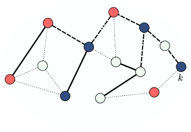
Figure 2: The clustered and linked topology that will result for the network shown in Fig. 1. The bold dashed lines depict the links used for relaying data among agents.

7 Simulation Results

We consider a fully connected network with 50 randomly distributed agents. The agents observe data originating from three different models ($C=3$). Each model $w_{{\cal C}_{m}}^{\circ}\in\mathbb{R}^{M\times 1}$ is generated as follows: $w^{\circ}_{\mathcal{C}_{m}}=[w_{r_{1}},\ldots,w_{r_{M}}]^{\intercal}$, with entries $w_{r_{c}}\in[1,-1]$. In our example we set $M=2$; larger values of $M$ are generally easier for clustering and, therefore, we illustrate the operation of the algorithm for $M=2$. The assignment of the agents to models is random. Agents having the same color belong to the same cluster. The maximum number of neighbors is $n_{\max}=6$. Every agent $k$ has access to a scalar measurement $\boldsymbol{d}_{k}(i)$ and a $1\times M$ regression vector $\boldsymbol{u}_{k,i}$. The measurements across the agents are assumed to be generated via the linear regression model $\boldsymbol{d}_{k}(i)=\boldsymbol{u}_{k,i}{w}_{k}^{\circ}+\boldsymbol{v}_{k}(i)$, where $\boldsymbol{v}_{k}(i)$ is measurement noise assumed to be a zero-mean white random process that is independent over space. It is also assumed that the regression data $\boldsymbol{u}_{k,i}$ is independent over space and independent of $\boldsymbol{v}_{\ell}(j)$ for all $k,\ell,i,j$. All random processes are assumed to be stationary. The statistical profile of the noise across the agents for $k=1,\ldots,N$ is shown in Fig. 3(a). The regressors are of size $M=2$ and have diagonal covariance matrices ${R}_{u,k}$ shown in Fig. 3(b). We set $\{\mu,\alpha,\nu,\delta,\gamma\}=\{0.05,0.015,0.98,0.17,0.5\}$. We use the uniform combination policy to generate the coefficients $\{a_{\ell k}(i)\}$.

\psfrag{V}[b]{\small$\sigma_{v,k}^{2}$}\psfrag{R}[b]{\small$\textrm{Tr}(R_{u,k})$}\includegraphics[width=240.0pt]{./figures/C_Noise.eps}

Figure 3: The statistical noise and signal profiles over the network.

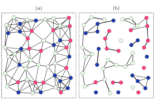
Figure 4: The network topology (a) and the clustered topology at steady-state (b).

Figure 4(a) shows the topology of one of 100 Monte Carlo experiments. Figure 4(b) presents the final topology after applying the clustering technique. Figure 5(a) depicts the simulated transient mean-square deviation (MSD) of the network compared to other clustering methods. The model assignments change at time instant $i=400$.

The normalized clustering errors of types I and II by each agent $k$ at time $i$ are given, respectively, by

$$\boldsymbol{v}_{\textrm{I},k}(i) \triangleq\frac{(\mathds{1}-{[\boldsymbol{E}_{i}]}_{:,k})^{\intercal}\times({[E^{\circ}]}_{:,k}-{[\boldsymbol{E}_{i}]}_{:,k})}{(n_{k}-1)}$$ (123)

$$\boldsymbol{v}_{\textrm{II},k}(i) \triangleq\frac{{[\boldsymbol{E}_{i}]}_{:,k}^{\intercal}\times({[\boldsymbol{E}_{i}]}_{:,k}-{[E^{\circ}]}_{:,k})}{(n_{k}-1)}$$ (124)

where $E^{\circ}$ is the true clustering matrix. Figures 6(a)–6(b) depict the normalized clustering errors $\overline{v}_{\textrm{I}}$ and $\overline{v}_{\textrm{II}}$ over the network.

\psfrag{simulated-Zhao}[bl]{ \scriptsize simulated \cite[cite]{[\@@bibref{}{cluster3}{}{}]}}\psfrag{simulated-Chen-CTA}[bl]{ \scriptsize simulated \cite[cite]{[\@@bibref{}{cluster4}{}{}]}}\psfrag{MSD-w}[bl]{ \scriptsize simulated (MSD)}\includegraphics[width=264.0pt]{./figures/C_MSD.eps}

Figure 5: The transient mean-square deviation (MSD) using different approaches.

\psfrag{Chen-CTA}[bl]{ \scriptsize\cite[cite]{[\@@bibref{}{cluster4}{}{}]} scheme}\psfrag{Zhao}[bl]{ \scriptsize\cite[cite]{[\@@bibref{}{cluster3}{}{}]} scheme}\psfrag{me}[bl]{ \scriptsize proposed scheme}\psfrag{v1}[bl]{ \small$\overline{v}_{\textrm{I}}$}\psfrag{v2}[bl]{ \small$\overline{v}_{\textrm{II}}$}\includegraphics[width=276.0pt]{./figures/C_Errors.eps}

Figure 6: The normalized clustering errors of types I and II over the network.

Using the same setup of the previous example, Fig. 7(a) shows the topology of one experiment with the clustering technique only. Figure 7(b) presents the final topology when we apply the clustering with linking technique. Figure 8 indicates the simulated transient mean-square deviation (MSD) of the agents with and without the linking technique. The normalized clustering errors over the network are shown in Fig. 9.

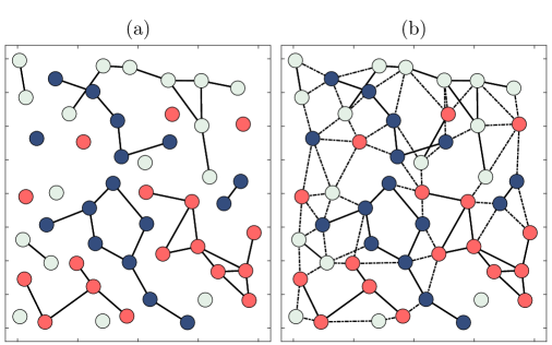
Figure 7: The clustered network topology at steady-state (a) and the clustered and linked topology at steady-state (b).

\psfrag{v1}[bl]{ \scriptsize$v_{\textrm{I}}$}\psfrag{v2}[bl]{ \scriptsize$v_{\textrm{II}}$}\psfrag{simulated with linking}[bl]{ \scriptsize clustering with linking}\psfrag{simulated without linking}[bl]{ \scriptsize clustering without linking}\includegraphics[width=312.0pt]{./figures/L_MSD.eps}

Figure 8: The transient mean-square deviation with and without applying the linking technique.

\psfrag{v1}[bl]{ \scriptsize$\overline{v}_{\textrm{I}}$}\psfrag{v2}[bl]{ \scriptsize$\overline{v}_{\textrm{II}}$}\psfrag{simulated with linking}[bl]{ \scriptsize Simulated with linking}\psfrag{simulated without linking}[bl]{\scriptsize Simulated without linking}\includegraphics[width=264.0pt]{./figures/L_Errors.eps}

Figure 9: The normalized clustering errors of types I and II over the network.

8 Conclusion

We proposed a distributed algorithm that carries out the tasks of estimation and clustering simultaneously with exponentially decaying error probabilities for false decisions. We showed how the agents choose the subset of their neighbors to cooperate with and turn off suspicious links. The simulations illustrate the performance of the proposed strategy and compare with other related works. We proposed an additional step to enhance the performance by linking, as much as possible, the agents that belonging to the same cluster and do not have direct links to connect them.

References

- [1] S. Khawatmi, A. M. Zoubir, and A. H. Sayed. Decentralized clustering over adaptive networks. In Proc. 23rd European Signal Processing Conference (EUSIPCO), pages 2745–2749, Nice, France, September 2015.
- [2] A. H. Sayed. Adaptive networks. In Proc. IEEE, volume 102, pages 460–497, April 2014.
- [3] A. H. Sayed. Adaptation, learning, and optimization over networks. Found. Trends in Mach. Learn., 7(4–5):311–801, July 2014.
- [4] J. B. Predd, S. B. Kulkarni, and H. V. Poor. Distributed learning in wireless sensor networks. IEEE Signal Processing Magazine, 23(4):56–69, July 2006.
- [5] A. Bertrand and M. Moonen. Distributed adaptive node-specific signal estimation in fully connected sensor networks, Part I: Sequential node updating. IEEE Trans. Signal Processing, 58(10):5277–5291, October 2010.
- [6] S. Chouvardas, K. Slavakis, and S. Theodoridis. Adaptive robust distributed learning in diffusion sensor networks. IEEE Trans. Signal Processing, 59(10):4692–4707, 2011.
- [7] A. Nedic and A. Ozdaglar. Distributed subgradient methods for multiagent optimization. IEEE Trans. Autom. Control, 54(1):48–61, January 2009.
- [8] S. Al-Sayed, A. M. Zoubir, and A. H Sayed. Robust adaptation in impulsive noise. IEEE Trans. on Signal Processing, 64(11):2851–2865, 2016.
- [9] J. Liu, M. Chu, and J. E. Reich. Multitarget tracking in distributed sensor networks. IEEE Signal Processing Mag., 24(3):36–46, 2007.
- [10] X. Zhang. Adaptive control and reconfiguration of mobile wireless sensor networks for dynamic multi-target tracking. IEEE Trans. Autom. Control, 56(10):2429–2444, 2011.
- [11] M. Z. Lin, M. N. Murthi, and K. Premaratne. Mobile adaptive networks for pursuing multiple targets. In Proc. IEEE International Conference on Acoust., Speech, and Signal Processing (ICASSP), pages 3217 – 3221, South Brisbane, QLD, Apr. 2015.
- [12] I. Francis and S. Chatterjee. Classification and estimation of several multiple regressions. The Annals of Statistics, 2(3):558–561, 1974.
- [13] L. Jacob, F. Bach, and J.-P. Vert. Clustered multi-task learning: A convex formulation. In Proc. Neural Inform. Processing Systems. (NIPS), pages 1–8, Vancouver, Canada, December 2008.
- [14] S. Y. Tu and A. H. Sayed. Distributed decision-making over adaptive networks. IEEE Trans. Signal Processing, 62(5):1054–1069, March 2014.
- [15] J. Chen, C. Richard, and A. H. Sayed. Multitask diffusion adaptation over networks. IEEE Trans. Signal Processing, 62(16):4129–4144, August 2014.
- [16] N. Bogdanovic, J. Plata-Chaves, and K. Berberidis. Distributed diffusion-based LMS for node-specific parameter estimation over adaptive netowrks. In Proc. IEEE International Conference on Acoust., Speech, and Signal Processing (ICASSP), pages 7223–7227, Florence, Italy, May 2014.
- [17] X. Zhao and A. H. Sayed. Clustering via diffusion adaptation over networks. In Proc. International Workshop on Cognitive Inform. Processing (CIP), pages 1–6, Baiona, Spain, May 2012.
- [18] J. Chen, C. Richard, and A. H. Sayed. Diffusion LMS over multitask networks. IEEE Trans. Signal Processing, 63(11):2733–2748, June 2015.
- [19] J. Chen, C. Richard, and A. H. Sayed. Adaptive clustering for multitask diffusion networks. In Proc. 23rd European Signal Processing Conference (EUSIPCO), pages 200–204, Nice, France, September 2015.
- [20] X. Zhao and A. H. Sayed. Distributed clustering and learning over networks. IEEE Trans. Signal Processing, 63(13):3285–3300, July 2015.
- [21] D. Bertsekas. Convex Analysis and Optimization. Athena Scientific, 2003.
- [22] S. Boyd and L. Vandenberghe. Convex Optimization. Cambridge University Press, 2004.
- [23] A. H. Sayed. Diffusion adaptation over networks. In R. Chellapa and S. Theodoridis, editors, Academic Press Library in Signal Processing, volume 3, pages 323–454. Academic Press, Elsevier, 2014.
- [24] O. Knill. Probability Theory and Stochastic Processes with Applications. Overseas Press India Private Limited, 2009.
- [25] A. Papoulis and S. U. Pillai. Probability, Random Variables, and Stochastic Processes. McGraw-Hill Higher Education, 2002.
- [26] J. Chen and A. H. Sayed. On the probability distribution of distributed optimization strategies. In Proc. Global Conference on Signal and Information Processing (GlobalSIP), pages 555–558, Austin, TX, December 2013.
- [27] J. Chen and A. H. Sayed. On the limiting behavior of distributed optimization strategies. In Proc. 50th Annual Allerton Conference on Communication, Control, and Computing, pages 1535–1542, Monticello, IL, October 2012.
- [28] X. Zhao and A. H. Sayed. Probability distribution of steady-state errors and adaptation over networks. In Proc. IEEE Statistical Signal Processing Workshop (SSP), pages 253–256, Nice, France, June 2011.
- [29] J. Sacks. Asymptotic distribution of stochastic approximation procedures. The Annals of Mathematical Statistics, 29(2):373–405, June 1958.
- [30] M. B. Nevelson and R. Z. Hasminskii. Stochastic approximation and recursive estimation. American Mathematical Society, 1976.
- [31] R. Bitmead. Convergence in distribution of LMS-type adaptive parameter estimates. IEEE Trans. Autom. Control, 28(1):54–60, January 1983.
- [32] A. H. Sayed. Adaptive Filters. Wiley, NJ, 2008.
- [33] B. Fristedt and L. Gray. A Modern Approach to Probability Theory. Birkhauser, Boston, MA, 1997.
- [34] P. Li, T. J. Hastie, and K. W. Church. Nonlinear estimators and tail bounds for dimension reduction in using Cauchy random projections. J. Mach. Learn. Res., 8:2497–2532, October 2007.
- [35] M. Chiani, D. Dardari, and M. K. Simon. New exponential bounds and approximations for the computation of error probability in fading channels. IEEE Trans. on Wireless Communications, 2(4):840–845, July 2003.