Emergence of Non-Axisymmetric Vortex in Strong-Coupling Chiral p-Wave Superconductor

Abstract

We studied strong-coupling effect upon an isolated vortex in a two-dimensional chiral p-wave superconductor. We solved the Eilenberger equation for the quasiclassical Green’s functions and the Éliashberg equation with single mode Einstein boson self-consistently. We calculated the free-energy of each obtained vortex, and found that a non-axisymmetric vortex metastably exists in some situation.

1 Introduction

The Migdal and Éliashberg theory of “strong-coupling superconductivity”Migdal1958 ; Eliashberg1960 ; Morel1962 has been very successful in qualitative description of superconductivity in real materialsScalapino1969 ; McMillan1969 ; Carbotte1990 . For example, it explains the deviation from the universal value $(2\Delta)/(k_{\text{B}}T_{\text{c}})\approx 3.53$ in Bardeen-Cooper-Schrieffer (BCS) theory, or the dependence of critical magnetic field on the transition temperature. Moreover, in some situation, it is known that the strong-coupling effect is not only a quantitative but also a qualitative effect (e.g., Refs. Marsiglio1991 ; Combescot1995 ). The strong-coupling effect modifies the spectrum of the quasiparticles. Therefore, one can expect that it may change the structure of low-energy states within the vortices in type-II superconductors. As far as we know, however, there have been only a few studies of the strong-coupling effect on a vortex on the basis of microscopic theories.

Two-dimensional chiral p-wave superconductivity is considered to be realized in Sr₂RuO₄ Maeno1994 ; Mackenzie2003 ; Sigrist2005 ; Maeno2012 . This state is topologically non-trivial and attracts much attention in these days. Within the vortices of this superconductor, reflected in the topology of this system, there is a zero-energy bound state, which is expected to be very robust against not-so-strong impuritiesVolovik1999 ; Matsumoto2000 ; Kato2000 ; Hayashi2005 ; Tanuma2009 ; Eschrig2009 ; Kurosawa2013 ; Kurosawa2015 ; Tanaka2016 . Recently, the relationship between this robustness and the odd-frequency pairing also has been discussedTanuma2009 ; Tanaka2016 ; Tanaka2012 .

In the present paper, we calculated the self-consistent Éliashberg equation to study how the strong-coupling feature affects the vortex of a chiral p-wave superconductor microscopically. We also calculated the free-energies of the vortices and discuss its stability.

2 Methods

In this study, we consider an isolated vortex in the two-dimensional spinless chiral p-wave superconductor with isotropic Fermi surface. We use quasiclassical theoryEilenberger1968 ; Larkin1968 ; we assume that the product of the coherence length of the superconductor $\xi$ and the Fermi wavevector $\vec{k}_{\text{F}}$ is much larger than unity. The quasiclassical Green’s function $\check{g}$ is a $2\times 2$ matrix and obeys the Eilenberger equation

$$\mathrm{i}\hbar\vec{v}_{\text{F}}\cdot\nabla\check{g}(\mathrm{i}\epsilon_{n},\alpha,\vec{r})+\left[\mathrm{i}\hbar\epsilon_{n}\check{\tau}_{3}+(q/c)\vec{v}_{\text{F}}\cdot\vec{A}\check{\tau}_{3}-\check{\Sigma}(\mathrm{i}\epsilon_{n},\alpha,\vec{r}),\;\check{g}(\mathrm{i}\epsilon_{n},\alpha,\vec{r})\right] =\check{0},$$ (1)

where $\epsilon_{n}=(2n+1)\pi k_{\text{B}}T/\hbar$ are the Matsubara frequencies, $\vec{v}_{\text{F}}$ is a Fermi velocity, $\alpha$ denotes a direction of momentum on the Fermi surface such that $\vec{k}=k_{\text{F}}(\cos\alpha,\sin\alpha)$, $\check{\tau}_{i}$ ($i=0,\dots 3$) are the Pauli matrices, $q$ is the elementary charge, $c$ is the speed of light, $\vec{A}$ is the vector potential, and

$$\check{\Sigma} =\begin{pmatrix}\sigma&\Delta\\ -{\Delta}^{*}&-\sigma\end{pmatrix},$$ (2)

is the self-energy. The quasiclassical Green’s function satisfies the normalization condition $\check{g}^{2}=-\pi^{2}\check{\tau}_{0}$ and its bulk value is

$$\check{g}=\frac{\pi}{\sqrt{-(\mathrm{i}\hbar\epsilon_{n}-\sigma)^{2}+\lvert\Delta\rvert^{2}}}\begin{pmatrix}-\mathrm{i}\hbar\epsilon_{n}+\sigma&\Delta\\ -{\Delta}^{*}&\mathrm{i}\hbar\epsilon_{n}-\sigma\end{pmatrix}.$$ (3)

To incorporate strong-coupling effect, we use Éliashberg equation to calculate the self-energy $\Sigma$ from the quasiclassical Green’s function;

$$\check{\Sigma}(\mathrm{i}\epsilon_{n},\alpha,\vec{r}) =N_{0}k_{\text{B}}T\sum_{\epsilon_{m}}^{\lvert\epsilon_{m}\rvert<\epsilon_{\text{c}}}\langle v(\mathrm{i}\epsilon_{n},\alpha,\mathrm{i}\epsilon_{m},\alpha^{\prime})\check{g}(\mathrm{i}\epsilon_{m},\alpha^{\prime},\vec{r})\rangle_{\alpha^{\prime}},$$ (4)

where $\epsilon_{\text{c}}$ is the cutoff of the Matsubara frequencies, $N_{0}$ is the density of states on the Fermi level, and $\langle\dots\rangle_{\alpha}$ denotes the average over the Fermi surface and is defined $\langle A(\alpha)\rangle_{\alpha}=\int_{0}^{2\pi}\mathrm{d}\alpha A(\alpha)/(2\pi)$. We took 47 equally spaced points in the momentum space. We assume that the interaction between electrons $v$ has the following form:

$$v(\mathrm{i}\epsilon_{n},\alpha,\mathrm{i}\epsilon_{m},\alpha^{\prime}) =\frac{C\omega_{0}^{2}}{(\epsilon_{n}-\epsilon_{m})^{2}+\omega_{0}^{2}}\times 2\cos(\alpha-\alpha^{\prime}),$$ (5)

where $\omega_{0}$ is a characteristic frequency of a mediated boson, and $C$ is a constant parameter. We set these parameters so that $\hbar\omega_{0}=3k_{\text{B}}T_{\text{c}}$, where $T_{\text{c}}$ is the critical temperature of the superconductivity. We choose this value so that the strong-coupling effect is very large but not unrealistic. We set the cutoff of the Matsubara frequencies $\hbar\epsilon_{\text{c}}=20k_{\text{B}}T_{\text{c}}$, and confirm that this cutoff is considered to be sufficiently large by comparison of the magnitude of the bulk pair-potential with those for $\hbar\epsilon_{\text{c}}=10k_{\text{B}}T_{\text{c}}$ and $15k_{\text{B}}T_{\text{c}}$. We also define $\xi_{0}=\hbar v_{\text{F}}/(k_{\text{B}}T_{\text{c}})$ and use it as a characteristic length of the spatial modulation of the self-energy.

The vector potential $\vec{A}$ is obtained from the quasiclassical Green’s function as

$$\nabla\times(\nabla\times\vec{A}) =\frac{q}{c}N_{0}k_{\text{B}}T\sum_{\epsilon_{n}}\operatorname{Tr}\langle\vec{v}_{\text{F}}\check{g}_{11}\rangle,$$ (6)

where $\operatorname{Tr}$ is a trace over the Nambu space. We define $\lambda_{0}=(N_{0}v_{\text{F}}^{2}q^{2}c^{-2})^{-1/2}$ as a characteristic length of the electromagnetic entities. We set $\lambda_{0}/\xi_{0}=2.5$ in this paper.

To discuss the stability of the isolated vortices, we calculated the free-energy deviation from the normal state $\Omega_{\text{sn}}$ with the following equation:

$$\Omega_{\text{sn}} =\int\mathrm{d}\vec{r}\left(N_{0}k_{\text{B}}T\sum_{\epsilon_{n}}\operatorname{Tr}\left\{\int_{0}^{1}\mathrm{d}s\langle\check{g}_{s}\check{\Sigma}\rangle-\frac{1}{2}\langle\check{g}\check{\Sigma}\rangle\right\}+\frac{B^{2}}{2}\right),$$ (7)

where $\vec{B}=\nabla\times\vec{A}$ is the magnetic field, and $\check{g}_{s}$ is a solution of

$$\mathrm{i}\hbar\vec{v}_{\text{F}}\cdot\nabla\check{g}_{s}+\left[\mathrm{i}\hbar\epsilon_{n}\check{\tau}_{3}+(q/c)\vec{v}_{\text{F}}\cdot\vec{A}\check{\tau}_{3}-s\check{\Sigma},\;\check{g}_{s}\right] =\check{0}, \check{g}_{s}^{2}=-\pi^{2}\check{\tau}_{0}.$$ (8)

The above expression of $\Omega_{\text{sn}}$ is a simple extension of the weak-coupling BCS oneSerene1983 ; Thuneberg1984 . We used the 15-points Gauss-Kronrod quadrature formula to integrate respect to $s$.

We numerically confirmed that the self-energy for Matsubara-frequencies $\check{\Sigma}(\mathrm{i}\epsilon_{n},\alpha,\vec{r})$ can be decoupled as

$$\check{\Sigma}(\mathrm{i}\epsilon_{n},\alpha,\vec{r}) =h(\mathrm{i}\epsilon_{n})\left[\check{\Sigma}_{+}(\vec{r})\mathrm{e}^{+\mathrm{i}\alpha}+\check{\Sigma}_{-}(\vec{r})\mathrm{e}^{-\mathrm{i}\alpha}\right],$$ (9)

and thus we show only the $\vec{r}$-dependent part $\check{\Sigma}_{+}(\vec{r})$ and $\check{\Sigma}_{-}(\vec{r})$ in the following section. At sufficiently far from the vortex, only $\check{\Sigma}_{+}$ or $\check{\Sigma}_{-}$ survives. Hereafter we assume that $\check{\Sigma}_{+}$ is a dominant part of the self-energy and survives in the bulk. As we can see in (9), Cooper pair of chiral p-wave superconductivity has internal angular momentum (chirality). If there is a vortex, two types of vortices can exist in this system; one type of vortex has vorticity (the angular momentum of vortex) parallel to the chirality, and the other type has vorticity anti-parallel to the chirality. In the present paper, we call the former “parallel vortex” and the latter “anti-parallel vortex”. In the Ginzburg-Landau(GL) theory, an anti-parallel vortex was shown to be more stable than a parallel vortexHeeb1999 .

To solve (1), we used so-called Riccati-parametrization methodNagato1993 ; Schpohl1995 and solved the parametrized differential equation with a 4th- and 5th-order adaptive Runge-Kutta method. We used the cylindrical coordinate system and took 48 equally spaced points on the azimuthal coordinates. To improve the accuracy of numerical integration of the free-energy, we used the composite Gauss-Lobatto quadrature to choose discrete points $r_{i}$ on the radial line. We divided the closed interval $[0,2.4]$ into 16 subintervals, applied the 7-points Gauss-Lobatto formula to each subinterval and obtained 97 discrete points $x_{i}$, and changed the variable as $r_{i}=x_{i}+x_{i}^{2}/2+x_{i}^{3}/3+x_{i}^{4}/4$ in order to make the sampling points denser near the center and more sparse far from the vortex. We calculated the self-energy from the quasiclassical Green’s functions via (4) and iterated the above until the self-energy sufficiently converged. After obtaining converged solution, we calculated the free-energy of vortices using (7). We changed initial profiles of the vortices so that the initial dominant- and induced- vortices were at separate positions, and repeated the same procedure as the above. Finally, we compared the resultant profiles and their free-energies to discuss stability.

3 Results and Discussion

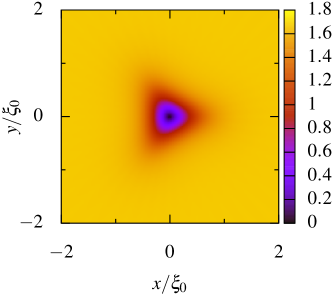
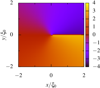
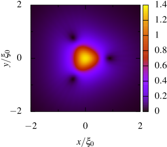
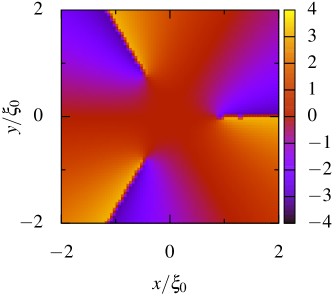
Figure 1: Profile of the off-diagonal part of the self-energy of the parallel vortex at $T=0.3T_{\text{c}}$ and $\hbar\epsilon_{n}=\pi k_{\text{B}}T$. Left-top: amplitude of dominant part ($h(\mathrm{i}\epsilon_{n})(\check{\Sigma}_{+})_{12}/T_{\text{c}}$), right-top: phase of dominant part ($\arg(\check{\Sigma}_{+})_{12}$), left-down: amplitude of induced part ($h(\mathrm{i}\epsilon_{n})(\check{\Sigma}_{-})_{12}/T_{\text{c}}$), right-down: phase of induced part ($\arg(\check{\Sigma}_{-})_{12}$). (Color figure online)

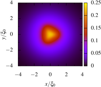
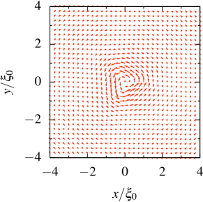
Figure 2: Electromagnetic quantities around the non-axisymmetric parallel vortex. Left: magnetic field, right: electric current density. (Color figure online)

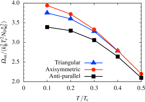
Figure 3: Free energy of each vortex. Red-circle: circular parallel vortex, blue-triangle: triangular parallel vortex, black-square: circular anti-parallel vortex. (Color figure online)

As for the anti-parallel vortices, we only obtained circular axisymmetric vortices for all temperature that we studied ($T/T_{\text{c}}=0.1$, $0.2$, $0.3$, $0.4$, and $0.5$), regardless of the initial profiles; in this case, the strong-coupling effect just modifies the shape of the vortex.

On the other hand, at moderately low temperatures, a non-axisymmetric solution emerges for parallel vortices, when the initial vortex sufficiently breaks the axisymmetry. Figure 1 shows the non-axisymmetric profile of dominant and induced parts of off-diagonal self-energy at $T/T_{\text{c}}=0.3$ and $\hbar\epsilon_{n}=\pi k_{\text{B}}T$. There the vortex of dominant component forms triangle and those of the induced component split into three. Figure 2 shows the current density around the vortex. We can confirm that the electromagnetic quantities also break the axisymmetry.

When we calculated parallel vortices at $T/T_{\text{c}}=0.5$, we found only an axisymmetric vortex: both circular and non-circular initial configurations of self-energy produce the same result. We thus conclude that unusual parallel vortices may not exist at high temperatures.

In Figure 3, we plot the free-energy of each vortex. We can see that at low temperatures, the non-axisymmetric vortex is more stable than symmetric one. We note that the symmetric anti-parallel vortex is more stable than the non-axisymmetric parallel vortex, at least under the parameters in this study.

There are many studies of non-axisymmetric vortices in spin triplet superfluids or superconductors with an isotropic Fermi surface. However, many of them have targeted vortices in the superfluid ³He-BThuneberg1986 ; Thuneberg1987 ; Salomaa1986 ; Fogelstroem1995 ; Tsutsumi2015 ; Silaev2015 ; Kondo1991 , or an f-wave superconductor similar to the ³He-BTsutsumi2012 ; these studies therefore cannot be compared with our work directly.

Tokuyasu, et al. have studied two-dimensional chiral p-wave superconductor within the GL theory in the weak- to strong-coupling regimesTokuyasu1990 . They have reported that non-axisymmetric vortices can emerge in some non-weak-coupling coefficients. However, the coefficients of the GL-functional of our target system fall into the same ones that we obtain in the weak-coupling limit (the $\beta$ parameter in Ref. Tokuyasu1990 is 0.5 in our system). Thus, the origin of non-axisymmetric vortices in our work is different from that of the previous work. This is also consistent with the fact that non-axisymmetric vortices only exist at low temperatures in the present work. Aoyama and Ikeda have reported that a vortex of ³He-A can be non-axisymmetric under the existence of anisotropic scatterersAoyama2010-JLTP ; Aoyama2010-PRB . Their model is different from ours, and the relationship between their and our results considered an important but remaining issue.

4 Conclusion

In this study, we numerically found that a non-axisymmetric vortex metastably exists in strong-coupling chiral p-wave superconductors. This anomalous vortex is more stable than the axisymmetric parallel one at sufficiently low temperatures, but symmetric anti-parallel vortex is still most stable. The emergence of this anomalous vortex is a consequence of the strong-coupling effect because we did not obtain such a vortex with the conventional weak-coupling gap equation. To clarify the underlying energetics that makes the non-axisymmetric vortex metastable is an interesting issue. The total phase diagram of this system is also left as a future issue.

- (1) A. B. Migdal, Sov. Phys. JETP 7, 996 (1958).
- (2) G. M. Éliashberg, Sov. Phys. JETP 11, 696 (1960).
- (3) P. Morel, P. W. Anderson, Phys. Rev. 125, 1263 (1962).
- (4) D. J. Scalapino, in Superconductivity, edited by R. D. Parks (Marcel Dekker, Inc., New York, 1969) p. 449.
- (5) W. L. McMillan, J. M. Rowell, in Superconductivity, edited by R. D. Parks (Marcel Dekker, Inc., New York, 1969) p. 561.
- (6) J. P. Carbotte, Rev. Mod. Phys. 62, 1027 (1990).
- (7) F. Marsiglio, J. P. Carbotte, Phys. Rev. B 43, 5355 (1991).
- (8) R. Combescot, Phys. Rev. B 51, 11625 (1995).
- (9) Y. Maeno, H. Hashimoto, K. Yoshida, S. Nishizaki, T. Fujita, J. G. Bednorz, F. Lichtenberg, Nature (London) 372, 532 (1994).
- (10) A. P. Mackenzie, Y. Maeno, Rev. Mod. Phys. 75, 657 (2003).
- (11) M. Sigrist, Prog. Theor. Phys. Suppl. 160, 1 (2005).
- (12) Y. Maeno, S. Kittaka, T. Nomura, S. Yonezawa, K. Ishida, J. Phys. Soc. Jpn. 81, 011009 (2012).
- (13) G. E. Volovik, JETP Lett. 70, 609 (1999).
- (14) M. Matsumoto, M. Sigrist, Physica B 281&282, 973 (2000).
- (15) Y. Kato, J. Phys. Soc. Jpn. 69, 3378 (2000).
- (16) N. Hayashi, Y. Kato, M. Sigrist, J. Low Temp. Phys. 139, 79 (2005).
- (17) Y. Tanuma, N. Hayashi, Y. Tanaka, A. A. Golubov, Phys. Rev. Lett. 102, 117003 (2009).
- (18) M. Eschrig, J. A. Sauls, New. J. Phys. 11, 075008 (2009).
- (19) N. Kurosawa, N. Hayashi, E. Arahata, Y. Kato, J. Low Temp. Phys. 175, 365 (2013).
- (20) N. Kurosawa, N. Hayashi, Y. Kato, J. Phys. Soc. Jpn. 84, 114710 (2015).
- (21) K. K. Tanaka, M. Ichioka, S. Onari, Phys. Rev. B 93, 094507 (2016).
- (22) Y. Tanaka, M. Sato, N. Nagaosa, J. Phys. Soc. Jpn. 81, 011013 (2012).
- (23) G. E. Eilenberger, Z. Phys. 214, 195 (1968).
- (24) A. I. Larkin, Yu. N. Ovchinnikov, Sov. Phys. JETP 28, 1200 (1968).
- (25) W. K. Park, J. L. Sarrao, J. D. Thompson, L. H. Greene, Phys. Rev. Lett. 100, 177001 (2008).
- (26) J. W. Serene, D. Rainer, Phys. Rep. 101, 221 (1983).
- (27) E. V. Thuneberg, J. Kurkijärvi, D. Rainer, Phys. Rev. B 29, 3913 (1984).
- (28) R. Heeb, D. F. Agterberg, Phys. Rev. B 59, 7076 (1999).
- (29) Y. Nagato, K. Nagai, J. Hara: J. Low Temp. Phys. 93, 33 (1993).
- (30) N. Schophol, K. Maki, Phys. Rev. B 52, 490 (1995).
- (31) E. V. Thuneberg, Phys. Rev. Lett. 56, 359 (1986).
- (32) E. V. Thuneberg, Phys. Rev. B 36, 3583 (1987).
- (33) M. M. Salomaa, G. E. Volovik, Phys. Rev. Lett. 56, 363 (1986).
- (34) M. Fogelström, J. Kurkijärvi, J. Low Temp. Phys. 98, 195 (1995).
- (35) Y. Tsutsumi, T. Kawakami, K. Shiozaki, M. Sato, K. Machida, Phys. Rev. B 91, 144504 (2015).
- (36) M. A. Silaev, E. Thuneberg, M. Fogelström, Phys. Rev. Lett. 115, 235301 (2015).
- (37) Y. Kondo, J. S. Korhonen, M. Krusius, V. V. Dmitriev, Y. M. Mukharsky, E. B. Sonin, G. E. Volovik, Phys. Rev. Lett. 67, 81 (1991).
- (38) Y. Tsutsumi, K. Machida, T. Ohmi, M. Ozawa, J. Phys. Soc. Jpn. 81, 074717 (2012).
- (39) K. Aoyama, R. Ikeda, J. Low Temp. Phys. 158, 404 (2010).
- (40) K. Aoyama, R. Ikeda, Phys. Rev. B 82, 144514 (2010).
- (41) T. A. Tokuyasu, D. W. Hess, J. A. Sauls, Phys. Rev. B 41, 8891 (1990).