Locally Adaptive Confidence Bands

Abstract

We develop honest and locally adaptive confidence bands for probability densities. They provide substantially improved confidence statements in case of inhomogeneous smoothness, and are easily implemented and visualized. The article contributes conceptual work on locally adaptive inference as a straightforward modification of the global setting imposes severe obstacles for statistical purposes. Among others, we introduce a statistical notion of local Hölder regularity and prove a correspondingly strong version of local adaptivity. We substantially relax the straightforward localization of the self-similarity condition in order not to rule out prototypical densities. The set of densities permanently excluded from the consideration is shown to be pathological in a mathematically rigorous sense. On a technical level, the crucial component for the verification of honesty is the identification of an asymptotically least favorable stationary case by means of Slepian’s comparison inequality.

T1Supported by the DFG Collaborative Research Center 823, Subproject C1, and DFG Research Grant RO 3766/4-1.

and

1 Introduction

Let $X_{1},\dots,X_{n}$ be independent real-valued random variables which are identically distributed according to some unknown probability measure $\mathbb{P}_{p}$ with Lebesgue density $p$. Assume that $p$ belongs to a nonparametric function class $\mathcal{P}$. For any interval $[a,b]$ and any significance level $\alpha\in(0,1)$, a confidence band for $p$, described by a family of random intervals $C_{n}(t,\alpha),t\in[a,b]$, is said to be (asymptotically) honest with respect to $\mathcal{P}$ if the coverage inequality

$$\liminf_{n}\inf_{p\in\mathcal{P}}\mathbb{P}^{\otimes n}_{p}\Big{(}p(t)\in C_{n}(t,\alpha)\text{ for all }\ t\in[a,b]\Big{)}\geq 1-\alpha$$

is satisfied. The aim of this article is to develop honest confidence bands $C_{n}(t,\alpha),t\in[a,b]$, with smallest possible width $|C_{n}(t,\alpha)|$ for every $t\in[a,b]$. Adaptive confidence sets maintain specific coverage probabilities over a large union of models while shrinking at the fastest possible nonparametric rate simultaneously over all submodels. If $\mathcal{P}$ is some class of densities within a union of Hölder balls $\mathcal{H}(\beta,L)$ with fixed radius $L>0$, the confidence band is called globally adaptive, cf. Cai and Low (2004), if for every $\beta>0$ and for every $\varepsilon>0$ there exists some constant $c>0$, such that

$$\limsup_{n}\sup_{p\in\mathcal{H}(\beta,L)\cap\mathcal{P}}\mathbb{P}^{\otimes n}_{p}\left(\sup_{t\in[a,b]}|C_{n}(t,\alpha)|\geq c\cdot r_{n}(\beta)\right)<\varepsilon.$$

Here, $r_{n}(\beta)$ denotes the minimax-optimal rate of convergence for estimation under supremum norm loss over $\mathcal{H}(\beta,L)\cap\mathcal{P}$, possibly inflated by additional logarithmic factors. However, if $\mathcal{P}$ equals the set of all densities contained in

$$\bigcup_{0<\beta\leq\beta^{*}}\mathcal{H}(\beta,L),$$

honest and adaptive confidence bands provably do not exist although adaptive estimation is possible. Indeed, Low (1997) shows that honest random-length intervals for a probability density at a fixed point cannot have smaller expected width than fixed-length confidence intervals with the size corresponding to the lowest regularity under consideration. Consequently, it is not even possible to construct a family of random intervals $C_{n}(t,\alpha),t\in[a,b]$, whose expected length shrinks at the fastest possible rate simultaneously over two distinct nested Hölder balls with fixed radius, and which is at the same time asymptotically honest for the union $\mathcal{P}$ of these Hölder balls. Numerous attempts have been made to tackle this adaptation problem in alternative formulations. Whereas Genovese and Wasserman (2008) relax the coverage property and do not require the confidence band to cover the function itself but a simpler surrogate function capturing the original function’s significant features, most of the approaches are based on a restriction of the parameter space. Under qualitative shape constraints, Hengartner and Stark (1995), Dümbgen (1998, 2003), and Davies, Kovac and Meise (2009) achieve adaptive inference. Within the models of nonparametric regression and Gaussian white noise, Picard and Tribouley (2000) succeeded to construct pointwise adaptive confidence intervals under a self-similarity condition on the parameter space, see also Kueh (2012) for thresholded needlet estimators. Under a similar condition, Giné and Nickl (2010) even develop asymptotically honest confidence bands for probability densities whose width is adaptive to the global Hölder exponent. Bull (2012) proved that a slightly weakened version of the self-similarity condition is necessary and sufficient. Kerkyacharian, Nickl and Picard (2012) develop corresponding results in the context of needlet density estimators on compact homogeneous manifolds. Under the same type of self-similarity condition, adaptive confidence bands are developed under a considerably generalized Smirnov-Bickel-Rosenblatt assumption based on Gaussian multiplier bootstrap, see Chernozhukov, Chetverikov and Kato (2014a). Hoffmann and Nickl (2011) introduce a nonparametric distinguishability condition, under which adaptive confidence bands exist for finitely many models under consideration. Their condition is shown to be necessary and sufficient.
Similar important conclusions concerning adaptivity in terms of confidence statements are obtained under Hilbert space geometry with corresponding $L^{2}$-loss, see Juditsky and Lambert-Lacroix (2003), Baraud (2004), Genovese and Wasserman (2005), Cai and Low (2006), Robins and van der Vaart (2006), Bull and Nickl (2013), and Nickl and Szabó (2016). Concerning $L^{p}$-loss, we also draw attention to Carpentier (2013).
In this article, we develop locally adaptive confidence bands. They provide substantially improved confidence statements in case of inhomogeneous smoothness. Conceptual work on locally adaptive inference is contributed as a straightforward modification of the global setting imposes severe obstacles for statistical purposes. It is already delicate to specify what a ”locally adaptive confidence band” should be. Disregarding any measurability issues, one possibility is to require a confidence band $C_{n,\alpha}=(C_{n,\alpha}(t))_{t\in[0,1]}$ to satisfy for every interval $U\subset[a,b]$ and for every $\beta$ (possibly restricted to a prescribed range)

$$\limsup_{n\to\infty}\sup_{\begin{subarray}{c}p\in{\mathcal{P}}:\\ p_{\arrowvert U_{\delta}}\in\mathcal{H}_{U_{\delta}}(\beta,L^{*})\end{subarray}}\mathbb{P}_{p}^{\otimes n}\left(|C_{n,\alpha}(t)|\geq\eta\,r_{n}(\beta)\text{ for some }t\in U\right)\rightarrow 0$$

as $\eta\to\infty$, where $U_{\delta}$ is the $\delta$-enlargement of $U$. However, this definition reflects a weaker notion of local adaptivity than the statistician may have in mind. On the other hand, we prove that, uniformly over the function class $\mathcal{P}$ under consideration, adaptation to the local or pointwise regularity in the sense of Daoudi, Lévy Véhel and Meyer (1998), Seuret and Lévy Véhel (2002) or Jaffard (1995, 2006) is impossible. Indeed, not even adaptive estimation with respect to pointwise regularity at a fixed point is achievable. On this way, we introduce a statistically suitable notion of local regularity $\beta_{n,p}(t),t\in[a,b]$, depending in particular on the sample size $n$. We prove a corresponding strong version of local adaptivity, while we substantially relax the straightforward localization of the global self-similarity condition in order not to rule out prototypical densities. The set of functions which is excluded from our parameter space diminishes for growing sample size and the set of permanently excluded functions is shown to be pathological in a mathematically rigorous sense. Our new confidence band appealingly relies on a discretized evaluation of a modified Lepski-type density estimator, including an additional supremum in the empirical bias term in the bandwidth selection criterion. A suitable discretization and a locally constant approximation allow to piece the pointwise constructions together in order to obtain a continuum of confidence statements. The complex construction makes the asymptotic calibration of the confidence band to the level $\alpha$ non-trivial. Whereas the analysis of the related globally adaptive procedure of Giné and Nickl (2010) reduces to the limiting distribution of the supremum of a stationary Gaussian process, our locally adaptive approach leads to a highly non-stationary situation. A crucial component is therefore the identification of a stationary process as a least favorable case by means of Slepian’s comparison inequality, subsequent to a Gaussian reduction using recent non-asymptotic techniques of Chernozhukov, Chetverikov and Kato (2014b). Due to the discretization, the band is computable and feasible from a practical point of view without losing optimality between the mesh points. Our results are exemplarily formulated in the density estimation framework but can be mimicked in other nonparametric models. To keep the representation concise we restrict the theory to locally adaptive kernel density estimators. The ideas can be transferred to wavelet estimators to a large extent as has been done for globally adaptive confidence bands in Giné and Nickl (2010).
The article is organized as follows. Basic notations are introduced in Section 2. Section 3 presents the main contributions, that is a substantially relaxed localized self-similarity condition in Subsection 3.1, the construction and in particular the asymptotic calibration of the confidence band in Subsection 3.2 as well as its strong local adaptivity properties in Subsection 3.3. Important supplementary results are postponed to Section 4, whereas Section 5 presents the proofs of the main results. Appendix A contains technical tools for the proofs of the main results.

2 Preliminaries and notation

Let $X_{1},\ldots,X_{n}$, $n\geq 4$, be independent random variables identically distributed according to some unknown probability measure $\mathbb{P}_{p}$ on $\mathbb{R}$ with continuous Lebesgue density $p$. Subsequently, we consider kernel density estimators

$$\hat{p}_{n}(\cdot,h)=\frac{1}{n}\sum_{i=1}^{n}K_{h}\left(X_{i}-\cdot\right)$$

with bandwidth $h>0$ and rescaled kernel $K_{h}(\cdot)=h^{-1}K(\cdot/h)$, where $K$ is a measurable and symmetric kernel with support contained in $[-1,1]$, integrating to one, and of bounded variation. Furthermore, $K$ is said to be of order $l\in\mathbb{N}$ if

$$\int x^{j}K(x)\mathop{\mathrm{\mathstrut d}}\nolimits\!x=0\ \text{ for }1\leq j\leq l,\quad\int x^{\l+1}K(x)\mathop{\mathrm{\mathstrut d}}\nolimits\!x=c\ \text{ with }c\neq 0.$$

For bandwidths of the form $h=c\cdot 2^{-j},j\in\mathbb{N}$, we abbreviate the notation writing $\hat{p}_{n}(\cdot,h)=\hat{p}_{n}(\cdot,j)$ and $K_{h}=K_{j}$. The open Euclidean ball of radius $r$ around some point $t\in\mathbb{R}$ is referred to as $B(t,r)$. Subsequently, the sample is split into two subsamples. For simplicity, we divide the sample into two parts of equal size $\tilde{n}=\lfloor n/2\rfloor$, leaving possibly out the last observation. Let

$$\chi_{1}=\{X_{1},\ldots,X_{\tilde{n}}\},\quad\chi_{2}=\{X_{\tilde{n}+1},\ldots,X_{2\tilde{n}}\}$$

be the distinct subsamples and denote by $\hat{p}_{n}^{(1)}(\cdot,h)$ and $\hat{p}_{n}^{(2)}(\cdot,h)$ the kernel density estimators with bandwidth $h$ based on $\chi_{1}$ and $\chi_{2}$, respectively. $\mathbb{E}_{p}^{\chi_{1}}$ and $\mathbb{E}_{p}^{\chi_{2}}$ denote the expectations with respect to the product measures

$$\mathbb{P}_{p}^{\chi_{1}} =\text{joint distribution of }X_{1},\ldots,X_{\tilde{n}},$$

$$\mathbb{P}_{p}^{\chi_{2}} =\text{joint distribution of }X_{\tilde{n}+1},\ldots,X_{2\tilde{n}},$$

respectively.
For some measure $Q$, we denote by $\|\cdot\|_{L^{p}(Q)}$ the $L^{p}$-norm with respect to $Q$. Is $Q$ the Lebesgue measure, we just write $\|\cdot\|_{p}$, whereas $\|\cdot\|_{\sup}$ denotes the uniform norm. For any metric space $(M,d)$ and subset $K\subset M$, we define the covering number $N(K,d,\varepsilon)$ as the minimum number of closed balls with radius at most $\varepsilon$ (with respect to $d$) needed to cover $K$. If the metric $d$ is induced by a norm $\Arrowvert\cdot\Arrowvert$, we write also $N(K,\|\cdot\|,\varepsilon)$ for $N(K,d,\varepsilon)$. As has been shown by Nolan and Pollard (1987) (Section 4 and Lemma 22), the class

$$\mathcal{K}=\left\{K\left(\frac{\cdot-t}{h}\right):t\in\mathbb{R},\,h>0\right\}$$

with constant envelope $\|K\|_{\sup}$ satisfies

$$N\left(\mathcal{K},\|\cdot\|_{L^{p}(Q)},\varepsilon\|K\|_{\sup}\right)\leq\left(\frac{A}{\varepsilon}\right)^{\nu},\quad 0<\varepsilon\leq 1,\quad p=1,2$$ (2.1)

for all probability measures $Q$ and for some finite and positive constants $A$ and $\nu$.
For $k\in\mathbb{N}$ we denote the $k$-th order Taylor polynomial of the function $p$ at point $y$ by $P^{p}_{y,k}$. Denoting furthermore by $\lfloor\beta\rfloor=\max\{n\in\mathbb{N}\cup\{0\}:n<\beta\}$, the Hölder class $\mathcal{H}_{U}(\beta)$ to the parameter $\beta>0$ on the open interval $U\subset\mathbb{R}$ is defined as the set of functions $p:U\to\mathbb{R}$ admitting derivatives up to the order $\lfloor\beta\rfloor$ and having finite Hölder norm

$$\|p\|_{\beta,U}=\sum_{k=0}^{\lfloor\beta\rfloor}\|p^{(k)}\|_{U}+\sup_{\begin{subarray}{c}x,y\,\in\,U\\ x\neq y\end{subarray}}\frac{|p^{(\lfloor\beta\rfloor)}(x)-p^{(\lfloor\beta\rfloor)}(y)|}{|x-y|^{\beta-\lfloor\beta\rfloor}}<\infty.$$

The corresponding Hölder ball with radius $L>0$ is denoted by $\mathcal{H}_{U}(\beta,L)$. With this definition of $\|\cdot\|_{\beta,U}$, the Hölder balls are nested, that is

$$\mathcal{H}_{U}(\beta_{2},L)\subset\mathcal{H}_{U}(\beta_{1},L)$$

for $0<\beta_{1}\leq\beta_{2}<\infty$ and $|U|<1$. Finally, $\mathcal{H}_{U}(\infty,L)=\bigcap_{\beta>0}\mathcal{H}_{U}(\beta,L)$ and $\mathcal{H}_{U}(\infty)=\bigcap_{\beta>0}\mathcal{H}_{U}(\beta)$. Subsequently, for any real function $f(\beta)$, the expression $f(\infty)$ is to be read as $\lim_{\beta\to\infty}f(\beta)$, provided that this limit exists. Additionally, the class of probability densities $p$, such that $p_{|U}$ is contained in the Hölder class $\mathcal{H}_{U}(\beta,L)$ is denoted by $\mathcal{P}_{U}(\beta,L)$. The indication of $U$ is omitted when $U=\mathbb{R}$.

3 Main results

In this section we pursue the new approach of locally adaptive confidence bands and present the main contribution of this article. A notion of local Hölder regularity tailored to statistical purposes, a corresponding condition of admissibility of a class of functions over which both asymptotic honesty and adaptivity (in a sense to be specified) can be achieved, as well as the construction of the new confidence band are presented. As compared to globally adaptive confidence bands, our confidence bands provide improved confidence statements for functions with inhomogeneous smoothness.

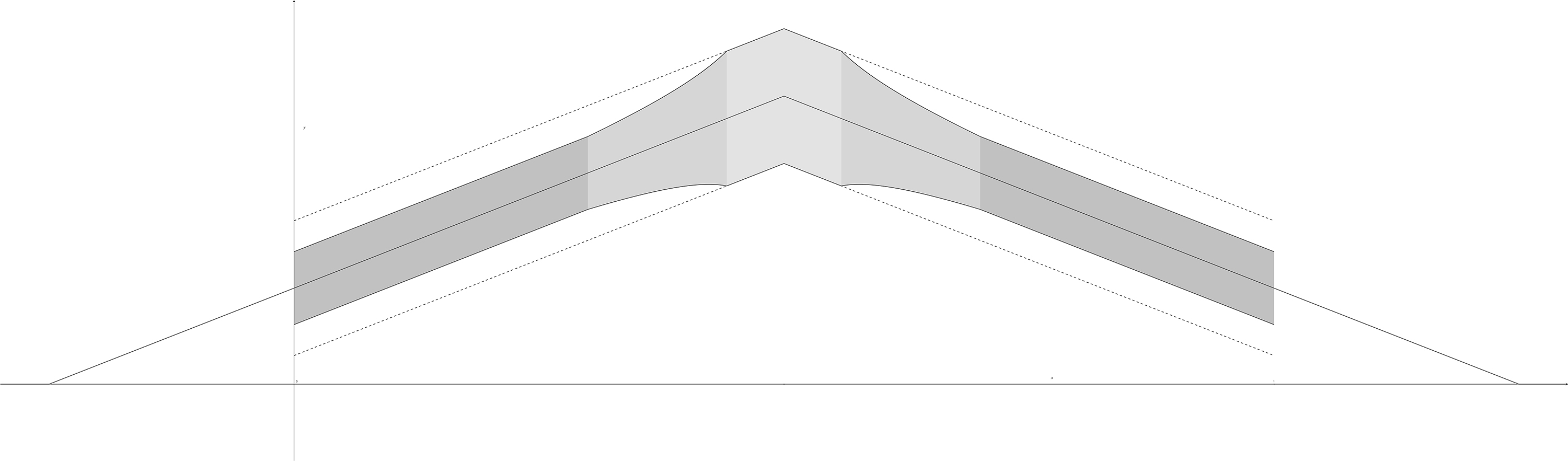
Figure 1: Comparison of locally and globally adaptive confidence bands

Figure 1 illustrates the kind of adaptivity that the construction should reveal. The shaded area sketches the intended locally adaptive confidence band as compared to the globally adaptive band (dashed line) for the triangular density and for fixed sample size $n$. This density is not smoother than Lipschitz at its maximal point but infinitely smooth at both sides. The region where globally and locally adaptive confidence bands coincide up to logarithmic factors (light gray regime in Figure 1) should shrink as the sample size increases, resulting in a substantial benefit of the locally adaptive confidence band outside of a shrinking neighborhood of the maximal point (dark grey regime together with a shrinking middle grey transition regime in Figure 1).

3.1 Admissible functions

As already pointed out in the introduction, no confidence band exists which is simultaneously honest and adaptive. It is necessary to impose a condition which guarantees the possibility of recovering the unknown smoothness parameter from the data. The subsequently introduced notion of admissibility aligns to the self-similarity condition as used in Picard and Tribouley (2000) and Giné and Nickl (2010) among others. Their self-similarity condition ensures that the data contains enough information to infer on the function’s regularity. As also emphasized in Nickl (2015), self-similarity conditions turn out to be compatible with commonly used adaptive procedures and have been shown to be sufficient and necessary for adaptation to a continuum of smoothing parameters in Bull (2012) when measuring the performance by the $L^{\infty}$-loss. Giné and Nickl (2010) consider globally adaptive confidence bands over the set

$$\bigcup_{\beta_{*}\leq\beta\leq\beta^{*}}\Bigg{\{}p\in\mathcal{P}(\beta,L):p\geq\delta\text{ on }[-\varepsilon,1+\varepsilon],\ \frac{c}{2^{j\beta}}\leq\|K_{j}\ast p-p\|_{\sup}\text{ for all }j\geq j_{0}\Bigg{\}}$$ (3.1)

for some constant $c>0$ and $0<\varepsilon<1$, where $\beta^{*}=l+1$ with $l$ the order of the kernel. They work on the scale of Hölder-Zygmund rather than Hölder classes. For this reason they include the corresponding bias upper bound condition which is not automatically satisfied for $\beta=\beta^{*}$ in that case.

Remark 1.

As mentioned in Giné and Nickl (2010), if $K(\cdot)=\frac{1}{2}\mathbbm{1}\{\cdot\in[-1,1]\}$ is the rectangular kernel, the set of all twice differentiable densities $p\in\mathcal{P}(2,L)$ that are supported in a fixed compact interval $[a,b]$ satisfies (3.1) with a constant $c>0$. The reason is that due to the constraint of being a probability density, $\|p^{\prime\prime}\|_{\sup}$ is bounded away from zero uniformly over this class, in particular $p^{\prime\prime}$ cannot vanish everywhere.

A localized version of the self-similarity condition characterizing the above class reads as follows.

For any nondegenerate interval $(u,v)\subset[0,1]$, there exists some $\beta\in[\beta_{*},\beta^{*}]$ with $p_{\arrowvert(u,v)}\in\mathcal{P}_{(u,v)}(\beta,L^{*})$ and

$$c\cdot 2^{-j\beta}\leq\sup_{s\in(u+2^{-j},v-2^{-j})}|(K_{j}\ast p)(s)-p(s)|$$ (3.2)

for all $j\geq j_{0}\vee\log_{2}(1/(v-u))$.

Remark 2.

Inequality (3.2) can be satisfied only for

$$\tilde{\beta}=\tilde{\beta}_{p}(U)=\sup\left\{\beta\in(0,\infty]:p_{|U}\in\mathcal{H}_{U}(\beta)\right\}.$$

The converse is not true, however.

$(i)$ There exist functions $p:U\to\mathbb{R}$, $U\subset\mathbb{R}$ some interval, which are not Hölder continuous to their exponent $\tilde{\beta}$. The Weierstraß function $W_{1}:U\to\mathbb{R}$ with

$$W_{1}(\cdot)=\sum_{n=0}^{\infty}2^{-n}\cos\left(2^{n}\pi\,\cdot\right)$$

is such an example. Indeed, Hardy (1916) proves that

$$W_{1}(x+h)-W_{1}(x)=O\left(|h|\log\left(\frac{1}{|h|}\right)\right),$$

which implies the Hölder continuity to any parameter $\beta<1$, hence $\tilde{\beta}\geq 1$. Moreover, he shows in the same reference that $W_{1}$ is nowhere differentiable, meaning that it cannot be Lipschitz continuous, that is $\tilde{\beta}=1$ but $W_{1}\notin\mathcal{H}_{U}(\tilde{\beta})$.

$(ii)$ It can also happen that $p_{|U}\in\mathcal{H}_{U}(\tilde{\beta})$ but

$$\limsup_{\delta\to 0}\sup_{\begin{subarray}{c}|x-y|\leq\delta\\ x,y\in U\end{subarray}}\frac{|p^{(\lfloor\tilde{\beta}\rfloor)}(x)-p^{(\lfloor\tilde{\beta}\rfloor)}(y)|}{|x-y|^{\tilde{\beta}-\lfloor\tilde{\beta}\rfloor}}=0,$$ (3.3)

meaning that the left-hand side of (3.2) is violated. In the analysis literature, the subset of functions in $\mathcal{H}_{U}(\tilde{\beta})$ satisfying (3.3) is called little Lipschitz (or little Hölder) space. As a complement of an open and dense set, it forms a nowhere dense subset of $\mathcal{H}_{U}(\tilde{\beta})$.

Due to the localization, a condition like (3.2) rules out examples which seem to be typical to statisticians. Assume that $K$ is a kernel of order $l$ with $l\geq 1$, and recall $\beta^{*}=l+1$. Then (3.2) excludes for instance the triangular density in Figure 1 because both sides are linear, in particular the second derivative exists and vanishes when restricted to an interval $U$ which does not contain the maximal point. In contrast to the observation in Remark 1, $\|p^{\prime\prime}\|_{U}$ may vanish for subintervals $U\subset[a,b]$. For the same reason, densities with a constant piece are excluded. In general, if $p$ restricted to the $2^{-j_{0}}$-enlargement of $U$ is a polynomial of order at most $l$, (3.2) is violated as the left-hand side is not equal to zero. In view of these deficiencies, a condition like (3.2) is insufficient for statistical purposes.

To circumvent this deficit, we introduce $\|\cdot\|_{\beta,\beta^{*},U}$ by

$$\|p\|_{\beta,\beta^{*},U}=\sum_{k=0}^{\lfloor\beta\wedge\beta^{*}\rfloor}\big{\|}p^{(k)}\big{\|}_{U}+\sup_{\begin{subarray}{c}x,y\,\in\,U\\ x\neq y\end{subarray}}\frac{\left|p^{(\lfloor\beta\wedge\beta^{*}\rfloor)}(x)-p^{(\lfloor\beta\wedge\beta^{*}\rfloor)}(y)\right|}{|x-y|^{\beta-\lfloor\beta\wedge\beta^{*}\rfloor}}$$ (3.4)

for $\beta>0$ and for some bounded open subinterval $U\subset\mathbb{R}$. As verified in Lemma A.7, $\|p\|_{\beta_{1},\beta^{*},U}\leq\|p\|_{\beta_{2},\beta^{*},U}$ for $0<\beta_{1}\leq\beta_{2}<\infty$ and $|U|\leq 1$. With the help of $\|\cdot\|_{\beta,\beta^{*},U}$, we formulate a localized self-similarity type condition in the subsequent Assumption 3.1, which does not exclude these prototypical densities as mentioned above. For any bounded open interval $U\subset\mathbb{R}$, let $\mathcal{H}_{\beta^{*},U}(\beta,L)$ be the set of functions $p:U\to\mathbb{R}$ admitting derivatives up to the order $\lfloor\beta\wedge\beta^{*}\rfloor$ with $\|p\|_{\beta,\beta^{*},U}\leq L$. Moreover, $\mathcal{H}_{\beta^{*},U}(\beta)$ is the set of functions $p:U\to\mathbb{R}$, such that $\|p\|_{\beta,\beta^{*},U}$ is well-defined and finite. Correspondingly, $\mathcal{H}_{\beta^{*},U}(\infty,L)=\bigcap_{\beta>0}\mathcal{H}_{\beta^{*},U}(\beta,L)$ and $\mathcal{H}_{\beta^{*},U}(\infty)=\bigcap_{\beta>0}\mathcal{H}_{\beta^{*},U}(\beta)$. Define furthermore

$$\beta_{p}(U)=\sup\left\{\beta\in(0,\infty]:p_{|U}\in\mathcal{H}_{\beta^{*},U}(\beta,L^{*})\right\}.$$ (3.5)

Remark 3.

If for some open interval $U\subset[0,1]$ the derivative $p_{|U}^{(\beta^{*})}$ exists and

$$p_{|U}^{(\beta^{*})}\equiv 0,$$

then $\|p\|_{\beta,\beta^{*},U}$ is finite uniformly over all $\beta>0$. If

$$p_{|U}^{(\beta^{*})}\not\equiv 0,$$

then $\beta^{*}$, $\|p\|_{\beta,\beta^{*},U}$ is finite if and only if $\beta\leq\beta^{*}$ as a consequence of the mean value theorem. That is, $\beta_{p}(U)\in(0,\beta^{*}]\cup\{\infty\}$.

Assumption 3.1.

For sample size $n\in\mathbb{N}$, some $0<\varepsilon<1$, $0<\beta_{*}<1$, and $L^{*}>0$, a density $p$ is said to be admissible if $p\in\mathcal{P}_{(-\varepsilon,1+\varepsilon)}(\beta_{*},L^{*})$ and the following holds true: for any $t\in[0,1]$ and for any $h\in\mathcal{G}_{\infty}$ with

$$\mathcal{G}_{\infty}=\{2^{-j}:j\in\mathbb{N},\,j\geq j_{\min}=\lceil 2\vee\log_{2}(2/\varepsilon)\rceil\},$$

there exists some $\beta\in[\beta_{*},\beta^{*}]\cup\{\infty\}$ such that the following conditions are satisfied for $u=h$ or $u=2h$:

$$p_{|B(t,u)}\in\mathcal{H}_{\beta^{*},B(t,u)}(\beta,L^{*})$$ (3.6)

and

$$\sup_{s\in B(t,u-g)}\left|(K_{g}\ast p)(s)-p(s)\right|\geq\frac{g^{\beta}}{\log n}$$ (3.7)

for all $g\in\mathcal{G}_{\infty}$ with $g\leq u/8$.

The set of admissible densities is denoted by $\mathscr{P}_{n}^{\operatorname{adm}}=\mathscr{P}_{n}^{\operatorname{adm}}(K,\beta_{*},L^{*},\varepsilon)$.

Lemma 3.2.

Any admissible density $p\in\mathscr{P}_{n}^{\operatorname{adm}}(K,\beta_{*},L^{*},\varepsilon)$ can satisfy (3.6) and (3.7) for $\beta=\beta_{p}(B(t,u))$ only.

By construction, the collection of admissible densities is increasing with the number of observations, that is $\mathscr{P}_{n}^{\operatorname{adm}}\subset\mathscr{P}_{n+1}^{\operatorname{adm}}$, $n\in\mathbb{N}$. The logarithmic denominator even weakens the assumption for growing sample size, permitting smaller and smaller Lipschitz constants.

Remark 4.

Assumption 3.1 does not require an admissible function to be totally ”unsmooth” everywhere. For instance, if $K$ is the rectangular kernel and $L^{*}$ is sufficiently large, the triangular density as depicted in Figure 1 is (eventually – for sufficiently large $n$) admissible. It is globally not smoother than Lipschitz, and the bias lower bound condition (3.7) is (eventually) satisfied for $\beta=1$ and pairs $(t,h)$ with $|t-1/2|\leq(7/8)h$. Although the bias lower bound condition to the exponent $\beta^{*}=2$ is not satisfied for any $(t,h)$ with $t\in[0,1]\setminus(1/2-h,1/2+h)$, these tuples $(t,h)$ fulfill (3.6) and (3.7) for $\beta=\infty$, which is not excluded anymore by the new Assumption 3.1. Finally, if the conditions (3.6) and (3.7) are not simultaneously satisfied for some pair $(t,h)$ with

$$\frac{7}{8}h<\left|t-\frac{1}{2}\right|<h,$$

then they are fulfilled for the pair $(t,2h)$ and $\beta=1$, because $|t-1/2|<(7/8)2h$.

In view of this remark, it is crucial not to require (3.6) and (3.7) to hold for every pair $(t,h)$. We now denote by

$$\mathscr{P}_{n} =\mathscr{P}_{n}(K,\beta_{*},L^{*},\varepsilon,M)=\left\{p\in\mathscr{P}_{n}^{\operatorname{adm}}(K,\beta_{*},L^{*},\varepsilon):\inf_{x\in[-\varepsilon,1+\varepsilon]}p(x)\geq M\right\}$$

the set of admissible densities being bounded below by $M>0$ on $[-\varepsilon,1+\varepsilon]$. We restrict our considerations to combinations of parameters for which the class $\mathscr{P}_{n}$ is non-empty.

The remaining results of this subsection are about the massiveness of the function classes $\mathscr{P}_{n}$. They are stated for the particular case of the rectangular kernel. Other kernels may be treated with the same idea; verification of (3.7) however appears to require a case-by-case analysis for different kernels. The following proposition demonstrates that the pointwise minimax rate of convergence remains unchanged when passing from the class $\mathcal{H}(\beta,L^{*})$ to $\mathscr{P}_{n}\cap\mathcal{H}(\beta,L^{*})$.

Proposition 3.3 (Lower pointwise risk bound).

For the rectangular kernel $K_{R}$ there exists some constant $M>0$, such that for any $t\in[0,1]$, for any $\beta\in[\beta_{*},1]$, for any $0<\varepsilon<1$, and for any $k\geq k_{0}(\beta_{*})$ there exists some $x>0$ and some $L(\beta)>0$ with

$$\inf_{T_{n}}\sup_{\begin{subarray}{c}p\in\mathscr{P}_{k}:\\ p_{|(-\varepsilon,1+\varepsilon)}\in\mathcal{H}_{(-\varepsilon,1+\varepsilon)}(\beta,L)\end{subarray}}\mathbb{P}_{p}^{\otimes n}\left(n^{\frac{\beta}{2\beta+1}}\left|T_{n}(t)-p(t)\right|\geq x\right)>0$$

for all $L\geq L(\beta)$, for the class $\mathscr{P}_{k}=\mathscr{P}_{k}(K_{R},\beta_{*},L^{*},\varepsilon,M)$, where the infimum is running over all estimators $T_{n}$ based on $X_{1},\dots,X_{n}$.

Note that the classical construction for the sequence of hypotheses in order to prove minimax lower bounds consists of a smooth density distorted by small $\beta$-smooth perturbations, properly scaled with the sample size $n$. However, there does not exist a fixed constant $c>0$, such that all of its members are contained in the class (3.1). Thus, the constructed hypotheses in our proof are substantially more complex, for which reason we restrict attention to $\beta\leq 1$.

Although Assumption 3.1 is getting weaker for growing sample size, some densities are permanently excluded from consideration. The following proposition states that the exceptional set of permanently excluded densities is pathological.

Proposition 3.4.

For the rectangular kernel $K_{R}(\cdot)=\frac{1}{2}\mathbbm{1}\{\cdot\in[-1,1]\}$, let

$$\mathscr{R}=\bigcup_{n\in\mathbb{N}}\mathscr{P}_{n}^{\operatorname{adm}}(K_{R},\beta_{*},L^{*},\varepsilon).$$

Then, for any $t\in[0,1]$, for any $h\in\mathcal{G}_{\infty}$ and for any $\beta\in[\beta_{*},1)$, the set

$$\mathcal{P}_{B(t,h)}(\beta,L^{*})\setminus\mathscr{R}_{|B(t,h)}$$

is nowhere dense in $\mathcal{P}_{B(t,h)}(\beta,L^{*})$ with respect to $\|\cdot\|_{\beta,B(t,h)}$.

Among more involved approximation steps, the proof reveals the existence of functions with the same regularity in the sense of Assumption 3.1 on every interval for $\beta\in(0,1)$. This property is closely related to but does not coincide with the concept of mono-Hölder continuity from the analysis literature, see for instance Barral et al. (2013). Hardy (1916) shows that the Weierstraß function is mono-Hölder continuous for $\beta\in(0,1)$. For any $\beta\in(0,1]$, the next lemma shows that Weierstraß’ construction

$$W_{\beta}(\cdot)=\sum_{n=0}^{\infty}2^{-n\beta}\cos(2^{n}\pi\,\cdot)$$ (3.8)

satisfies the bias condition (3.7) for the rectangular kernel to the exponent $\beta$ on any subinterval $B(t,h)$, $t\in[0,1]$, $h\in\mathcal{G}_{\infty}$.

Lemma 3.5.

For all $\beta\in(0,1)$, the Weierstraß function $W_{\beta}$ as defined in (3.8) satisfies $W_{\beta|U}\in\mathcal{H}_{U}(\beta,L_{W})$ with some Lipschitz constant $L_{W}=L_{W}(\beta)$ for every open interval $U$. For the rectangular kernel $K_{R}$ and $\beta\in(0,1]$, the Weierstraß function fulfills the bias lower bound condition

$$\sup_{s\in B(t,h-g)}\left|(K_{R,g}\ast W_{\beta})(s)-W_{\beta}(s)\right| >\left(\frac{4}{\pi}-1\right)g^{\beta}$$

for any $t\in\mathbb{R}$ and for any $g,h\in\mathcal{G}_{\infty}$ with $g\leq h/2$.

The whole scale of parameters $\beta\in[\beta_{*},1]$ in Proposition 3.4 can be covered by passing over from Hölder classes to Hölder-Zygmund classes in the definition of $\mathscr{P}_{n}$. Although the Weierstraß function $W_{1}$ in (3.8) is not Lipschitz, a classical result, see Heurteaux (2005) or Mauldin and Williams (1986) and references therein, states that $W_{1}$ is indeed contained in the Zygmund class $\Lambda_{1}$. That is, it satisfies

$$|W_{1}(x+h)-W_{1}(x-h)-2W_{1}(x)|\leq C|h|$$

for some $C>0$ and for all $x\in\mathbb{R}$ and for all $h>0$. Due to the symmetry of the rectangular kernel $K_{R}$, it therefore fulfills the bias upper bound

$$\left\|K_{R,g}\ast W_{1}-W_{1}\right\|_{\sup}\leq C^{\prime}g^{\beta}\ \ \ \text{for all $g\in(0,1]$}.$$

The local adaptivity theory can be likewise developed on the scale of Hölder-Zygmund rather than Hölder classes – here, we restrict attention to Hölder classes because they are commonly considered in the theory of kernel density estimation.

3.2 Construction of the confidence band

The new confidence band is based on a kernel density estimator with variable bandwidth incorporating a localized but not the fully pointwise Lepski (1990) bandwidth selection procedure. A suitable discretization and a locally constant approximation allow to piece the pointwise constructions together in order to obtain a continuum of confidence statements. The complex construction makes the asymptotic calibration of the confidence band to the level $\alpha$ non-trivial. Whereas the analysis of the related globally adaptive procedure of Giné and Nickl (2010) reduces to the limiting distribution of the supremum of a stationary Gaussian process, our locally adaptive approach leads to a highly non-stationary situation. An essential component is therefore the identification of a stationary process as a least favorable case by means of Slepian’s comparison inequality.

We now describe the procedure. The interval $[0,1]$ is discretized into equally spaced grid points, which serve as evaluation points for the locally adaptive estimator. We discretize by a mesh of width

$$\delta_{n}=\left\lceil 2^{\frac{j_{\min}}{\beta_{*}}}\left(\frac{\log\tilde{n}}{\tilde{n}}\right)^{-\kappa_{1}}(\log\tilde{n})^{\frac{2}{\beta_{*}}}\right\rceil^{-1}$$

with $\kappa_{1}\geq 1/(2\beta_{*})$ and set $\mathcal{H}_{n}=\{k\delta_{n}:k\in\mathbb{Z}\}$. Fix now constants

$$c_{1}>\frac{2}{\beta_{*}\log 2}\quad\text{and}\quad\kappa_{2}>c_{1}\log 2+4.$$ (3.9)

Consider the set of bandwidth exponents

$$\mathcal{J}_{n}=\left\{j\in\mathbb{N}\ :\ j_{\min}\leq j\leq j_{\max}=\left\lfloor\log_{2}\left(\frac{\tilde{n}}{(\log\tilde{n})^{\kappa_{2}}}\right)\right\rfloor\right\}.$$

The bound $j_{\min}$ ensures that $2^{-j}\leq\varepsilon\wedge(1/4)$ for all $j\in\mathcal{J}_{n}$, and therefore avoids that infinite smoothness in (3.14) and the corresponding local parametric rate is only attainable in trivial cases as the interval under consideration is $[0,1]$. The bound $j_{\max}$ is standard and particularly guarantees consistency of the kernel density estimator with minimal bandwidth within the dyadic grid of bandwidths

$$\mathcal{G}_{n}=\Big{\{}2^{-j}:j\in\mathcal{J}_{n}\Big{\}}.$$

We define the set of admissible bandwidths for $t\in[0,1]$ as

$$\begin{split}\mathcal{A}_{n}(t)=\Big{\{}j\in\mathcal{J}_{n}:\max_{s\in B\left(t,\frac{7}{8}\cdot 2^{-j}\right)\cap\mathcal{H}_{n}}\left|\hat{p}_{n}^{(2)}(s,m)-\hat{p}_{n}^{(2)}(s,m^{\prime})\right|\leq c_{2}\sqrt{\frac{\log\tilde{n}}{\tilde{n}2^{-m}}}\\ \text{ for all }m,m^{\prime}\in\mathcal{J}_{n}\text{ with }m>m^{\prime}>j+2\Big{\}},\end{split}$$ (3.10)

with constant $c_{2}=c_{2}(A,\nu,\beta_{*},L^{*},K,\varepsilon)$ specified in the proof of Proposition 4.1. Furthermore, let

$$\hat{j}_{n}(t)=\min\mathcal{A}_{n}(t),\quad t\in[0,1],$$ (3.11)

and $\hat{h}_{n}(t)=2^{-\hat{j}_{n}(t)}$. Note that a slight difference to the classical Lepski procedure is the additional maximum in (3.10), which reflects the idea of adapting localized but not completely pointwise for fixed sample size $n$. The bandwidth (3.11) is determined for all mesh points $k\delta_{n},k\in T_{n}=\{1,\ldots,\delta_{n}^{-1}\}$ in $[0,1]$, and set piecewise constant in between. Accordingly, with

$$\hat{h}_{n,1}^{loc}(k) =2^{-\hat{j}_{n}((k-1)\delta_{n})-u_{n}},\quad\hat{h}_{n,2}^{loc}(k)=2^{-\hat{j}_{n}(k\delta_{n})-u_{n}},$$

where $u_{n}=c_{1}\log\log\tilde{n}$ is some sequence implementing the undersmoothing, the estimators are defined as

$$\begin{split}\hat{h}_{n}^{loc}(t)&=\hat{h}_{n,k}^{loc}=\min\left\{\hat{h}_{n,1}^{loc}(k),\hat{h}_{n,2}^{loc}(k)\right\}\qquad\text{and}\\ \hat{p}_{n}^{loc}(t,h)&=\hat{p}_{n}^{(1)}(k\delta_{n},h)\end{split}$$ (3.12)

for $t\in I_{k}=[(k-1)\delta_{n},k\delta_{n})$, $k\in T_{n}\setminus\{\delta_{n}^{-1}\}$, $I_{\delta_{n}^{-1}}=[1-\delta_{n},1]$. The following theorem lays the foundation for the construction of honest and locally adaptive confidence bands.

Theorem 3.1 (Least favorable case).

For the estimators defined in (3.12) and normalizing sequences

$$a_{n}=c_{3}(-2\log\delta_{n})^{1/2},\quad b_{n}=\frac{3}{c_{3}}\left\{(-2\log\delta_{n})^{1/2}-\frac{\log(-\log\delta_{n})+\log 4\pi}{2(-2\log\delta_{n})^{1/2}}\right\},$$

with $c_{3}=\sqrt{2}/TV(K)$, it holds

$$\liminf_{n\to\infty}\inf_{p\in\mathscr{P}_{n}}\mathbb{P}_{p}^{\otimes n}\left(a_{n}\left(\sup_{t\in[0,1]}\sqrt{\tilde{n}\hat{h}_{n}^{loc}(t)}\left|\hat{p}_{n}^{loc}(t,\hat{h}_{n}^{loc}(t))-p(t)\right|-b_{n}\right)\leq x\right)$$

$$\hskip 227.62204pt\geq 2\,\mathbb{P}\Big{(}\sqrt{L^{*}}G\leq x\Big{)}-1$$

for some standard Gumbel distributed random variable $G$.

The proof of Theorem 3.1 is based on several completely non-asymptotic approximation techniques. The asymptotic Komlós-Major-Tusnády-approximation technique, used in Giné and Nickl (2010), has been evaded using non-asymptotic Gaussian approximation results recently developed in Chernozhukov, Chetverikov and Kato (2014b). The essential component of the proof of Theorem 3.1 is the application of Slepian’s comparison inequality to reduce considerations from a non-stationary Gaussian process to the least favorable case of a maximum of $\delta_{n}^{-1}$ independent and identical standard normal random variables.

With $q_{1-\alpha/2}$ denoting the $(1-\alpha/2)$-quantile of the standard Gumbel distribution, we define the confidence band as the family of piecewise constant random intervals $C_{n,\alpha}=(C_{n,\alpha}(t))_{t\in[0,1]}$ with

$$\begin{split}C_{n,\alpha}(t)=\left[\hat{p}_{n}^{loc}(t,\hat{h}_{n}^{loc}(t))-\frac{q_{n}(\alpha)}{\sqrt{\tilde{n}\hat{h}_{n}^{loc}(t)}},\ \ \hat{p}_{n}^{loc}(t,\hat{h}_{n}^{loc}(t))+\frac{q_{n}(\alpha)}{\sqrt{\tilde{n}\hat{h}_{n}^{loc}(t)}}\right]\end{split}$$ (3.13)

and

$$q_{n}(\alpha)=\frac{\sqrt{L^{*}}\cdot q_{1-\alpha/2}}{a_{n}}+b_{n}.$$

For fixed $\alpha>0$, $q_{n}(\alpha)=O(\sqrt{\log n})$ as $n$ goes to infinity.

Corollary 3.2 (Honesty).

The confidence band as defined in (3.13) satisfies

$$\liminf_{n\to\infty}\inf_{p\in\mathscr{P}_{n}}\mathbb{P}_{p}^{\otimes n}\Big{(}p(t)\in C_{n,\alpha}(t)\text{ for every }t\in[0,1]\Big{)}\,\geq\,1-\alpha.$$

3.3 Local Hölder regularity and local adaptivity

In the style of global adaptivity in connection with confidence sets one may call a confidence band $C_{n,\alpha}=(C_{n,\alpha}(t))_{t\in[0,1]}$ locally adaptive if for every interval $U\subset[0,1]$,

$$\limsup_{n\to\infty}\sup_{p\in{\mathscr{P}_{n}}_{\arrowvert U_{\delta}}\cap\mathcal{H}_{\beta^{*},U_{\delta}}(\beta,L^{*})}\mathbb{P}_{p}^{\chi_{2}}\Big{(}|C_{n,\alpha}(t)|\geq\eta\cdot r_{n}(\beta)\text{ for some }t\in U\Big{)}\rightarrow 0$$

as $\eta\to\infty$, for every $\beta\in[\beta_{*},\beta^{*}]$, where $U_{\delta}$ is the open $\delta$-enlargement of $U$. As a consequence of the subsequently formulated Theorem 3.7, our confidence band satisfies this notion of local adaptivity up to a logarithmic factor. However, in view of the imagination illustrated in Figure 1 the statistician aims at a stronger notion of adaptivity, where the asymptotic statement is not formulated for an arbitrary but fixed interval $U$ only. Precisely, the goal would be to adapt even to some pointwise or local Hölder regularity, two well established notions from analysis.

Definition 3.3 (Pointwise Hölder exponent, Seuret and Lévy Véhel (2002)).

Let $p:\mathbb{R}\to\mathbb{R}$ be a function, $\beta>0$, $\beta\notin\mathbb{N}$, and $t\in\mathbb{R}$. Then $p\in\mathcal{H}_{t}(\beta)$ if and only if there exists a real $R>0$, a polynomial $P$ with degree less than $\lfloor\beta\rfloor$, and a constant $c$ such that

$$|p(x)-P(x-t)|\leq c|x-t|^{\beta}$$

for all $x\in B(t,R)$. The pointwise Hölder exponent is denoted by

$$\beta_{p}(t)=\sup\{\beta:p\in\mathcal{H}_{t}(\beta)\}.$$

Definition 3.4 (Local Hölder exponent, Seuret and Lévy Véhel (2002)).

a
Let $p:\Omega\to\mathbb{R}$ be a function and $\Omega\subset\mathbb{R}$ an open set. One classically says that $p\in\mathcal{H}_{loc}(\beta,\Omega)$, where $0<\beta<1$, if there exists a constant $c$ such that

$$\left|p(x)-p(y)\right|\leq c|x-y|^{\beta}$$

for all $x,y\in\Omega$. If $m<\beta<m+1$ for some $m\in\mathbb{N}$, then $p\in\mathcal{H}_{loc}(\beta,\Omega)$ means that there exists a constant $c$ such that

$$\left|\partial^{m}p(x)-\partial^{m}p(y)\right|\leq c|x-y|^{\beta-m}$$

for all $x,y\in\Omega$. Set now

$$\beta_{p}(\Omega)=\sup\{\beta:p\in\mathcal{H}_{loc}(\beta,\Omega)\}.$$

Finally, the local Hölder exponent in $t$ is defined as

$$\beta_{p}^{loc}(t)=\sup\{\beta_{p}(O_{i}):i\in I\},$$

where $(O_{i})_{i\in I}$ is a decreasing family of open sets with $\cap_{i\in I}O_{i}=\{t\}$. [By Lemma 2.1 in Seuret and Lévy Véhel (2002), this notion is well defined, that is, it does not depend on the particular choice of the decreasing sequence of open sets.]

The next proposition however shows that attaining the minimax rates of convergence corresponding to the pointwise or local Hölder exponent (possibly inflated by some logarithmic factor) uniformly over $\mathscr{P}_{n}$ is an unachievable goal.

Proposition 3.5.

For the rectangular kernel $K_{R}$ there exists some constant $M>0$, such that for any $t\in[0,1]$, for any $\beta\in[\beta_{*},1]$, for any $0<\varepsilon<1$, and for any $k\geq k_{0}(\beta_{*})$ there exists some $x>0$ and constants $L=L(\beta)>0$ and $c_{4}=c_{4}(\beta)>0$ with

$$\inf_{T_{n}}\sup_{p\in\mathscr{S}_{k}(\beta)}\mathbb{P}_{p}^{\otimes n}\left(n^{\frac{\beta}{2\beta+1}}\left|T_{n}(t)-p(t)\right|\geq x\right)>0\ \ \ \text{for all $k\geq k_{0}(\beta_{*})$}$$

with

$$\mathscr{S}_{k}(\beta) =\mathscr{S}_{k}(L,\beta,\beta_{*},M,K_{R},\varepsilon)$$

$$=\Big{\{}p\in\mathscr{P}_{k}(K_{R},\beta_{*},L,\varepsilon,M):\exists\,r\geq c_{4}\,n^{-\frac{1}{2\beta+1}}$$

$$\hskip 71.13188pt\text{ such that }\,p_{|B(t,r)}\in\mathcal{H}_{B(t,r)}(\infty,L)\Big{\}}\cap\mathcal{H}_{(-\varepsilon,1+\varepsilon)}(\beta,L),$$

where the infimum is running over all estimators $T_{n}$ based on $X_{1},\dots,X_{n}$.

The proposition furthermore reveals that if a density $p\in\mathscr{P}_{k}$ is Hölder smooth to some exponent $\eta>\beta$ on a ball around $t$ with radius at least of the order $n^{-1/(2\beta+1)}$, then no estimator for $p(t)$ can achieve a better rate than $n^{-\beta/(2\beta+1)}$. We therefore introduce an $n$-dependent statistical notion of local regularity for any point $t$. Roughly speaking, we intend it to be the maximal $\beta$ such that the density attains this Hölder exponent within $B(t,h_{\beta,n})$, where $h_{\beta,n}$ is of the optimal adaptive bandwidth order $(\log n/n)^{1/(2\beta+1)}$. We realize this idea with $\|\cdot\|_{\beta,\beta^{*},U}$ as defined in (3.4) and used in Assumption 3.1.

Definition 3.6 ($n$-dependent local Hölder exponent).

With the classical optimal bandwidth within the class $\mathcal{H}(\beta)$

$$h_{\beta,n}=2^{-j_{\min}}\cdot\left(\frac{\log\tilde{n}}{\tilde{n}}\right)^{\frac{1}{2\beta+1}},$$

define the class $\mathcal{H}_{\beta^{*},n,t}(\beta,L)$ as the set of functions $p:B(t,h_{\beta,n})\to\mathbb{R}$, such that $p$ admits derivatives up to the order $\lfloor\beta\wedge\beta^{*}\rfloor$ and $\|p\|_{\beta,\beta^{*},B(t,h_{\beta,n})}\leq L$, and $\mathcal{H}_{\beta^{*},n,t}(\beta)$ the class of functions $p:B(t,h_{\beta,n})\to\mathbb{R}$ for which $\|p\|_{\beta,\beta^{*},B(t,h_{\beta,n})}$ is well-defined and finite. The $n$-dependent local Hölder exponent for the function $p$ at point $t$ is defined as

$$\beta_{n,p}(t)=\sup\Big{\{}\beta>0:p_{|B(t,h_{\beta,n})}\in\mathcal{H}_{\beta^{*},n,t}(\beta,L^{*})\Big{\}}.$$ (3.14)

If the supremum is running over the empty set, we set $\beta_{n,p}(t)=0$.

Finally, the next theorem shows that the confidence band adapts to the $n$-dependent local Hölder exponent.

Theorem 3.7 (Strong local adaptivity).

There exists some $\gamma=\gamma(c_{1})$, such that

$$\limsup_{n\to\infty}\sup_{p\in\mathscr{P}_{n}}\mathbb{P}_{p}^{\chi_{2}}\left(\sup_{t\in[0,1]}|C_{n,\alpha}(t)|\cdot\left(\frac{\log\tilde{n}}{\tilde{n}}\right)^{-\frac{\beta_{n,p}(t)}{2\beta_{n,p}(t)+1}}\geq(\log\tilde{n})^{\gamma}\right)=0.$$

Note that the case $\beta_{n,p}(t)=\infty$ is not excluded in the formulation of Theorem 3.7. That is, if $p_{|U}$ can be represented as a polynomial of degree strictly less than $\beta^{*}$, the confidence band attains even adaptively the parametric width $n^{-1/2}$, up to logarithmic factors. In particular, the band can be tighter than $n^{-\beta^{*}/(2\beta^{*}+1)}$. In general, as long as $\delta\leq\varepsilon$ and $B(t,h_{\beta^{*},n})\subset U_{\delta}$,

$$\beta_{n,p}(t)\geq\beta_{p}(U_{\delta})\quad\text{ for all }t\in U.$$

Corollary 3.8 (Weak local adaptivity).

For every interval $U\subset[0,1]$,

$$\limsup_{n\to\infty}\sup_{p\in{\mathscr{P}_{n}}_{\arrowvert U_{\delta}}\cap\mathcal{H}_{\beta^{*},U_{\delta}}(\beta,L^{*})}\mathbb{P}_{p}^{\chi_{2}}\left(\sup_{t\in U}|C_{n,\alpha}(t)|\geq\left(\frac{\log\tilde{n}}{\tilde{n}}\right)^{\frac{\beta}{2\beta+1}}(\log\tilde{n})^{\gamma}\right)$$

is equal to zero for every $\beta\in[\beta_{*},\beta^{*}]$, where $U_{\delta}$ is the open $\delta$-enlargement of $U$ and $\gamma$ as in Theorem 3.7.

4 Supplementary notation and results

The following auxiliary results are crucial ingredients in the proofs of Theorem 3.1 and Theorem 3.7.
Recalling the quantity $h_{\beta,n}$ in Definition 3.6, Proposition 4.1 shows that $2^{-\hat{j}_{n}(\cdot)}$ lies in a band around

$$\bar{h}_{n}(\cdot)=h_{\beta_{n,p}(\cdot),n}$$ (4.1)

uniformly over all admissible densities $p\in\mathscr{P}_{n}$. Proposition 4.1 furthermore reveals the necessity to undersmooth, which has been already discovered by Bickel and Rosenblatt (1973), leading to a bandwidth deflated by some logarithmic factor. Set now

$$\bar{j}_{n}(\cdot)=\left\lfloor\log_{2}\left(\frac{1}{\bar{h}_{n}(\cdot)}\right)\right\rfloor+1,$$

such that the bandwidth $2^{-\bar{j}_{n}(\cdot)}$ is an approximation of $\bar{h}_{n}(\cdot)$ by the next smaller bandwidth on the grid $\mathcal{G}_{n}$ with

$$\frac{1}{2}\bar{h}_{n}(\cdot)\leq 2^{-\bar{j}_{n}(\cdot)}\leq\bar{h}_{n}(\cdot).$$

The next proposition states that the procedure chooses a bandwidth which simultaneously in the location $t$ is neither too large nor too small.

Proposition 4.1.

The bandwidth $\hat{j}_{n}(\cdot)$ defined in (3.11) satisfies

$$\lim_{n\to\infty}\sup_{p\in\mathscr{P}_{n}}\left\{1-\mathbb{P}_{p}^{\chi_{2}}\left(\hat{j}_{n}(k\delta_{n})\in\Big{[}k_{n}(k\delta_{n}),\,\bar{j}_{n}(k\delta_{n})+1\Big{]}\text{ for all }k\in T_{n}\right)\right\}=0$$

where $k_{n}(\cdot)=\bar{j}_{n}(\cdot)-m_{n}$, and $m_{n}=\frac{1}{2}c_{1}\log\log\tilde{n}$.

Lemma 4.2.

Let $s,t\in[0,1]$ be two points with $s<t$, and let $z\in(s,t)$. If

$$|s-t|\leq\frac{1}{8}\,h_{\beta_{*},n}$$ (4.2)

then

$$\frac{1}{3}\,\bar{h}_{n}(z)\leq\min\left\{\bar{h}_{n}(s),\bar{h}_{n}(t)\right\}\leq 3\,\bar{h}_{n}(z).$$

Lemma 4.3.

There exist positive and finite constants $c_{5}=c_{5}(A,\nu,K)$ and $c_{6}=c_{6}(A,\nu,L^{*},K)$, and some $\eta_{0}=\eta_{0}(A,\nu,L^{*},K)>0$, such that

$$\sup_{p\in\mathscr{P}_{n}}\mathbb{P}_{p}^{\chi_{i}}\left(\sup_{s\in\mathcal{H}_{n}}\max_{h\in\mathcal{G}_{n}}\sqrt{\frac{\tilde{n}h}{\log\tilde{n}}}\Big{|}\hat{p}_{n}^{(i)}(s,h)-\mathbb{E}_{p}^{\chi_{i}}\hat{p}_{n}^{(i)}(s,h)\Big{|}>\eta\right)\leq c_{5}\tilde{n}^{-c_{6}\eta},\quad i=1,2$$

for sufficiently large $n\geq n_{0}(A,\nu,L^{*},K)$ and for all $\eta\geq\eta_{0}$.

The next lemma states extends the classical upper bound on the bias for the modified Hölder classes $\mathcal{H}_{\beta^{*},B(t,U)}(\beta,L)$.

Lemma 4.4.

Let $t\in\mathbb{R}$ and $g,h>0$. Any density $p:\mathbb{R}\to\mathbb{R}$ with $p_{|B(t,g+h)}\in\mathcal{H}_{\beta^{*},B(t,g+h)}(\beta,L)$ for some $0<\beta\leq\infty$ and some $L>0$ satisfies

$$\sup_{s\in B(t,g)}\left|(K_{h}\ast p)(s)-p(s)\right|\leq b_{2}h^{\beta}$$ (4.3)

for some positive and finite constant $b_{2}=b_{2}(L,K)$.

Lemma 4.5.

For symmetric kernels $K$ and $\beta=1$, the bias bound (4.3) continues to hold if the Lipschitz balls are replaced by the corresponding Zygmund balls.

5 Proofs

We first prove the results of Section 3 in Subsection 5.1 and afterwards proceed with the proofs of the results Section 4 in Subsection 5.2.
For the subsequent proofs we recall the following notion of the theory of empirical processes.

Definition 5.1.

A class of measurable functions $\mathscr{H}$ on a measure space $(S,\mathscr{S})$ is a $Vapnik$-$\check{C}ervonenkis$ $class$ (VC class) of functions with respect to the envelope $H$ if there exists a measurable function $H$ which is everywhere finite with $\sup_{h\in\mathscr{H}}|h|\leq H$ and finite numbers $A$ and $v$, such that

$$\sup_{Q}N\Big{(}\mathscr{H},\|\cdot\|_{L^{2}(Q)},\varepsilon\|H\|_{L^{2}(Q)}\Big{)}\leq\left(\frac{A}{\varepsilon}\right)^{v}$$

for all $0<\varepsilon<1$, where the supremum is running over all probability measures $Q$ on $(S,\mathscr{S})$ for which $\|H\|_{L^{2}(Q)}<\infty$.

Nolan and Pollard (1987) call a class $Euclidean$ with respect to the envelope $H$ and with characteristics $A$ and $\nu$ if the same holds true with $L^{1}(Q)$ instead of $L^{2}(Q)$. The following auxiliary lemma is a direct consequence of the results in the same reference.

Lemma 5.2.

If a class of measurable functions $\mathscr{H}$ is Euclidean with respect to a constant envelope $H$ and with characteristics $A$ and $\nu$, then the class

$$\tilde{\mathscr{H}}=\left\{h-\mathbb{E}_{\mathbb{P}}h:h\in\mathscr{H}\right\}$$

is a VC class with envelope $2H$ and characteristics $A^{\prime}=4\sqrt{A}\vee 2A$ and $\nu^{\prime}=3\nu$ for any probability measure $\mathbb{P}$.

Proof 5.3.

For any probability measure $\mathbb{P}$ and for any functions $\tilde{h}_{1}=h_{1}-\mathbb{E}_{\mathbb{P}}h_{1}$, $\tilde{h}_{2}=h_{2}-\mathbb{E}_{\mathbb{P}}h_{2}\in\tilde{\mathscr{H}}$ with $h_{1},h_{2}\in\mathscr{H}$, we have

$$\|\tilde{h}_{1}-\tilde{h}_{2}\|_{L^{2}(Q)}\leq\|h_{1}-h_{2}\|_{L^{2}(Q)}+\|h_{1}-h_{2}\|_{L^{1}(\mathbb{P})}.$$

For any $0<\varepsilon\leq 1$, we obtain as a direct consequence of Lemma 14 in Nolan and Pollard (1987)

$$\begin{split}&N\left(\tilde{\mathscr{H}},L^{2}(Q),2\varepsilon\|H\|_{L^{2}(Q)}\right)\\ &\hskip 56.9055pt\leq N\left(\mathscr{H},L^{2}(Q),\frac{\varepsilon\|H\|_{L^{2}(Q)}}{2}\right)\cdot N\left(\mathscr{H},L^{1}(\mathbb{P}),\frac{\varepsilon\|H\|_{L^{1}(\mathbb{P})}}{2}\right).\end{split}$$ (5.1)

Nolan and Pollard (1987), page 789, furthermore state that the Euclidean class $\mathscr{H}$ is also a VC class with respect to the envelope $H$ and with

$$N\left(\mathscr{H},L^{2}(Q),\frac{\varepsilon\|H\|_{L^{2}(Q)}}{2}\right)\leq\left(\frac{4\sqrt{A}}{\varepsilon}\right)^{2\nu},$$

whereas

$$N\left(\mathscr{H},L^{1}(\mathbb{P}),\frac{\varepsilon\|H\|_{L^{1}(\mathbb{P})}}{2}\right)\leq\left(\frac{2A}{\varepsilon}\right)^{\nu}.$$

Inequality (5.1) thus implies

$$N\left(\tilde{\mathscr{H}},L^{2}(Q),2\varepsilon\|H\|_{L^{2}(Q)}\right)\leq\left(\frac{4\sqrt{A}\vee 2A}{\varepsilon}\right)^{3\nu}.$$

5.1 Proofs of the results in Section 3

Proof 5.4 (Proof of Lemma 3.2).

Let $p\in\mathscr{P}_{n}^{\operatorname{adm}}(K,\beta_{*},L^{*},\varepsilon)$ be an admissible density. That is, for any $t\in[0,1]$ and for any $h\in\mathcal{G}_{\infty}$ there exists some $\beta\in[\beta_{*},\beta^{*}]\cup\{\infty\}$, such that for $u=h$ or $u=2h$ both

$$p_{|B(t,u)}\in\mathcal{H}_{\beta^{*},B(t,u)}(\beta,L^{*})$$

and

$$\sup_{s\in B(t,u-g)}\left|(K_{g}\ast p)(s)-p(s)\right|\geq\frac{g^{\beta}}{\log n}\quad\text{ for all }g\in\mathcal{G}_{\infty}\text{ with }g\leq u/8$$

hold. By definition of $\beta_{p}(B(t,u))$ in (3.5), we obtain $\beta_{p}(B(t,u))\geq\beta$. We now prove by contradiction that also $\beta_{p}(B(t,u))\leq\beta$. If $\beta=\infty$, the proof is finished. Assume now that $\beta<\infty$ and that $\beta_{p}(B(t,u))>\beta$. Then, by Lemma A.7, there exists some $\beta<\beta^{\prime}<\beta_{p}(B(t,u))$ with $p_{|B(t,u)}\in\mathcal{H}_{\beta^{*},B(t,u)}(\beta^{\prime},L^{*})$. By Lemma 4.4, there exists some constant $b_{2}=b_{2}(L^{*},K)$ with

$$b_{2}g^{\beta^{\prime}}\geq\sup_{s\in B(t,u-g)}\left|(K_{g}\ast p)(s)-p(s)\right|\geq\frac{g^{\beta}}{\log n}$$

for all $g\in\mathcal{G}_{\infty}$ with $g\leq u/8$, which is a contradiction.

Proof 5.5 (Proof of Proposition 3.3).

The proof is based on a reduction of the supremum over the class to a maximum over two distinct hypotheses.

Part 1

For $\beta\in[\beta_{*},1)$, the construction of the hypotheses is based on the Weierstraß function as defined in (3.8) and is depicted in Figure 2. Consider the function $p_{0}:\mathbb{R}\to\mathbb{R}$ with

$$p_{0}(x)=\begin{cases}0,\quad&\text{if }\ |x-t|\geq\frac{10}{3}\\ \frac{1}{4}+\frac{3}{16}(x-t+2),\quad&\text{if }\ -\frac{10}{3}<x-t<-2\\ \frac{1}{6}+\frac{1-2^{-\beta}}{12}W_{\beta}(x-t),\quad&\text{if }\ |x-t|\leq 2\\ \frac{1}{4}-\frac{3}{16}(x-t-2),\quad&\text{if }\ 2<x-t<\frac{10}{3}\\ \end{cases}$$

and the function $p_{1,n}:\mathbb{R}\to\mathbb{R}$ with

$$p_{1,n}(x)=p_{0}(x)+q_{t+\frac{9}{4},n}(x)-q_{t,n}(x),\quad x\in\mathbb{R},$$

where

$$q_{a,n}(x)=\begin{cases}0,\quad&\text{if }\ |x-a|>g_{\beta,n}\\ \frac{1-2^{-\beta}}{12}\Big{(}W_{\beta}(x-a)-W_{\beta}(g_{\beta,n})\Big{)},\quad&\text{if }\ |x-a|\leq g_{\beta,n}\end{cases}$$

for $g_{\beta,n}=\frac{1}{4}n^{-1/(2\beta+1)}$ and $a\in\mathbb{R}$. Note that $p_{1,n|B(t,g_{\beta,n})}$ is constant with value

$$p_{1,n}(x)=\frac{1}{6}+\frac{1-2^{-\beta}}{12}W_{\beta}(g_{\beta,n})\quad\text{ for all }x\in B(t,g_{\beta,n}).$$

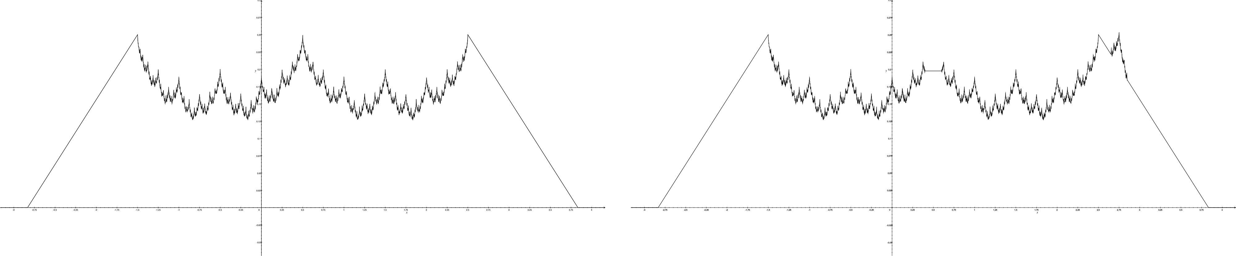
Figure 2: Functions $p_{0}$ and $p_{1,n}$ for $t=0.5$, $\beta=0.5$ and $n=100$

We now show that both $p_{0}$ and $p_{1,n}$ are contained in the class $\mathscr{P}_{k}$ for sufficiently large $k\geq k_{0}(\beta_{*})$ with

$$p_{0|(-\varepsilon,1+\varepsilon)},\,p_{1,n|(-\varepsilon,1+\varepsilon)}\in\mathcal{H}_{(-\varepsilon,1+\varepsilon)}(\beta,L^{*}).$$

$(i)$ We first verify that $p_{0}$ integrates to one. Then, it follows directly that also $p_{1,n}$ integrates to one. We have

$$\int p_{0}(x)\mathop{\mathrm{\mathstrut d}}\nolimits\!x =\int_{t-\frac{10}{3}}^{t-2}\left(\frac{1}{4}+\frac{3}{16}(x-t+2)\right)\mathop{\mathrm{\mathstrut d}}\nolimits\!x$$

$$\qquad+\int_{t-2}^{t+2}\left(\frac{1}{6}+\frac{1-2^{-\beta}}{12}W_{\beta}(x-t)\right)\mathop{\mathrm{\mathstrut d}}\nolimits\!x$$

$$\qquad+\int_{t+2}^{t+\frac{10}{3}}\left(\frac{1}{4}-\frac{3}{16}(x-t-2)\right)\mathop{\mathrm{\mathstrut d}}\nolimits\!x$$

$$=\frac{1}{6}+\frac{2}{3}+\frac{1-2^{-\beta}}{12}\int_{-2}^{2}W_{\beta}(x)\mathop{\mathrm{\mathstrut d}}\nolimits\!x+\frac{1}{6}$$

$$=1,$$

where the last equality is due to

$$\int_{-2}^{2}W_{\beta}(x)\mathop{\mathrm{\mathstrut d}}\nolimits\!x=\sum_{k=0}^{\infty}2^{-k\beta}\int_{-2}^{2}\cos(2^{k}\pi x)\mathop{\mathrm{\mathstrut d}}\nolimits\!x=0.$$

$(ii)$ Next, we check the non-negativity of $p_{0}$ and $p_{1,n}$ to show that they are probability density functions. We prove non-negativity for $p_{0}$, whereas non-negativity of $p_{1,n}$ is an easy implication. Since $p_{0}(-10/3)=0$ and $p_{0}$ is linear on $(t-10/3,t-2)$ with positive derivative, $p_{0}$ is non-negative on $(t-10/3,t-2)$. Analogously, $p_{0}$ is non-negative on $(t+2,t+10/3)$. Note furthermore that

$$|W_{\beta}(x)|\leq W_{\beta}(0)=\sum_{k=0}^{\infty}2^{-k\beta}=\frac{1}{1-2^{-\beta}}$$ (5.2)

for all $x\in\mathbb{R}$. Thus, for any $x\in\mathbb{R}$ with $|x-t|\leq 2$, we have

$$p_{0}(x)=\frac{1}{6}+\frac{1-2^{-\beta}}{12}W_{\beta}(x-t)\geq\frac{1}{6}-\frac{1}{12}=\frac{1}{12}>0.$$

$(iii)$ As $p_{0}$ and also $p_{1,n}$ are bounded from below by $M=1/12$ on $B(t,2)$, we furthermore conclude that they are bounded from below by $M$ on $(-1,2)\subset B(t,2)$, and therefore on any interval $[-\varepsilon,1+\varepsilon]$ with $0<\varepsilon<1$.

$(iv)$ We now verify that $p_{0|(-\varepsilon,1+\varepsilon)},\,p_{1,n|(-\varepsilon,1+\varepsilon)}\in\mathcal{H}_{(-\varepsilon,1+\varepsilon)}(\beta,L(\beta))$ for some positive constant $L(\beta)$. Note again that for any $0<\varepsilon<1$ and any $t\in[0,1]$, the inclusion $(-\varepsilon,1+\varepsilon)\subset B(t,2)$ holds. Thus,

$$\sup_{\begin{subarray}{c}x,y\in(-\varepsilon,1+\varepsilon)\\ x\neq y\end{subarray}}\frac{|p_{0}(x)-p_{0}(y)|}{|x-y|^{\beta}}=\frac{1-2^{-\beta}}{12}\cdot\sup_{\begin{subarray}{c}x,y\in(-\varepsilon,1+\varepsilon)\\ x\neq y\end{subarray}}\frac{|W_{\beta}(x-t)-W_{\beta}(y-t)|}{|(x-t)-(y-t)|^{\beta}},$$

which is bounded by some constant $c(\beta)$ according to Lemma 3.5. Together with (5.2) and with the triangle inequality, we obtain that

$$p_{0|(-\varepsilon,1+\varepsilon)}\in\mathcal{H}_{(-\varepsilon,1+\varepsilon)}(\beta,L)$$

for some Lipschitz constant $L=L(\beta)$. The Hölder continuity of $p_{1,n}$ is now a simple consequence. The function $p_{1,n}$ is constant on $B(t,g_{\beta,n})$ and coincides with $p_{0}$ on $(-\varepsilon,1+\varepsilon)\setminus B(t,g_{\beta,n})$. Hence, it remains to investigate combinations of points $x\in(-\varepsilon,1+\varepsilon)\setminus B(t,g_{\beta,n})$ and $y\in B(t,g_{\beta,n})$. Without loss of generality assume that $x\leq t-g_{\beta,n}$. Then,

$$\frac{|p_{1,n}(x)-p_{1,n}(y)|}{|x-y|^{\beta}}=\frac{|p_{1,n}(x)-p_{1,n}(t-g_{\beta,n})|}{|x-y|^{\beta}}\leq\frac{|p_{1,n}(x)-p_{1,n}(t-g_{\beta,n})|}{|x-(t-g_{\beta,n})|^{\beta}}\leq L,$$

which proves that also

$$p_{1,n|(-\varepsilon,1+\varepsilon)}\in\mathcal{H}_{(-\varepsilon,1+\varepsilon)}(\beta,L).$$

$(v)$ Finally, we address the verification of Assumption 3.1 for the hypotheses $p_{0}$ and $p_{1,n}$. Again, for any $t^{\prime}\in[0,1]$ and any $h\in\mathcal{G}_{\infty}$ the inclusion $B(t^{\prime},2h)\subset B(t,2)$ holds, such that in particular

$$p_{0|B(t^{\prime},h)}\in\mathcal{H}_{\beta^{*},B(t^{\prime},h)}(\beta,L_{W}(\beta))$$

for any $t^{\prime}\in[0,1]$ and for any $h\in\mathcal{G}_{\infty}$ by Lemma 3.5. Simultaneously, Lemma 3.5 implies

$$\sup_{s\in B(t^{\prime},h-g)}\left|(K_{R,g}\ast p_{0})(s)-p_{0}(s)\right|>\frac{1-2^{-\beta_{*}}}{12}\left(\frac{4}{\pi}-1\right)g^{\beta}\geq\frac{g^{\beta}}{\log k}$$

for all $g\leq h/2$ and for sufficiently large $k\geq k_{0}(\beta_{*})$. That is, for any $t^{\prime}\in[0,1]$, both (3.6) and (3.7) are satisfies for $p_{0}$ with $u=h$ for any $h\in\mathcal{G}_{\infty}$.
Concerning $p_{1,n}$ we distinguish between several combinations of pairs $(t^{\prime},h)$ with $t^{\prime}\in[0,1]$ and $h\in\mathcal{G}_{\infty}$.

$(v.1)$ If $B(t^{\prime},h)\cap B(t,g_{\beta,n})=\emptyset$, the function $p_{1,n}$ coincides with $p_{0}$ on $B(t^{\prime},h)$, for which Assumption 3.1 has been already verified.

$(v.2)$ If $B(t^{\prime},h)\subset B(t,g_{\beta,n})$, the function $p_{1,n}$ is constant on $B(t^{\prime},h)$, such that (3.6) and (3.7) trivially hold for $u=h$ and $\beta=\infty$.

$(v.3)$ If $B(t^{\prime},h)\cap B(t,g_{\beta,n})\neq\emptyset$ and $B(t^{\prime},h)\not\subset B(t,g_{\beta,n})$, we have that $t^{\prime}+h>t+g_{\beta,n}$ or $t^{\prime}-h<t-g_{\beta,n}$. As $p_{1,n|B(t,2)}$ is symmetric around $t$ we assume $t^{\prime}+h>t+g_{\beta,n}$ without loss of generality. In this case,

$$(t^{\prime}+2h-g)-(t+g_{\beta,n})>2\left(\frac{h}{2}-g\right),$$

such that

$$B\left(t^{\prime}+\frac{3}{2}h,\frac{h}{2}-g\right)\subset B(t^{\prime},2h-g)\setminus B(t,g_{\beta,n}).$$

Consequently, we obtain

$$\sup_{s\in B(t^{\prime},2h-g)}\left|(K_{R,g}\ast p_{1,n})(s)-p_{1,n}(s)\right|\geq\sup_{s\in B\left(t^{\prime}+\frac{3}{2}h,\frac{h}{2}-g\right)}\left|(K_{R,g}\ast p_{1,n})(s)-p_{1,n}(s)\right|.$$

If $2h\geq 8g$, we conclude that $h/2\geq 2g$, so that Lemma 3.5 finally proves Assumption 3.1 for $u=2h$ to the exponent $\beta$ for sufficiently large $k\geq k_{0}(\beta_{*})$.

Combining $(i)-(v)$, we conclude that $p_{0}$ and $p_{1,n}$ are contained in the class $\mathscr{P}_{k}$ with $p_{0|(-\varepsilon,1+\varepsilon)},p_{1,n|(-\varepsilon,1+\varepsilon)}\in\mathcal{H}_{(-\varepsilon,1+\varepsilon)}(\beta,L^{*})$ for sufficiently large $k\geq k_{0}(\beta_{*})$. The absolute distance of the two hypotheses in $t$ is at least

$$|p_{0}(t)-p_{1,n}(t)| =\frac{1-2^{-\beta}}{12}\left(W_{\beta}(0)-W_{\beta}(g_{\beta,n})\right)$$

$$=\frac{1-2^{-\beta}}{12}\sum_{k=0}^{\infty}2^{-k\beta}\left(1-\cos(2^{k}\pi g_{\beta,n})\right)$$

$$\geq\frac{1-2^{-\beta_{*}}}{12}2^{-\tilde{k}\beta}\left(1-\cos(2^{\tilde{k}}\pi g_{\beta,n})\right)$$

$$\geq 2c_{7}\,g_{\beta,n}^{\beta}$$ (5.3)

where $\tilde{k}\in\mathbb{N}$ is chosen such that $2^{-(\tilde{k}+1)}<g_{\beta,n}\leq 2^{-\tilde{k}}$ and

$$c_{7}=c_{7}(\beta_{*})=\frac{1-2^{-\beta_{*}}}{24}.$$

It remains to bound the distance between the associated product probability measures $\mathbb{P}_{0}^{\otimes n}$ and $\mathbb{P}_{1,n}^{\otimes n}$. For this purpose, we analyze the Kullback-Leibler divergence between these probability measures, which can be bounded from above by

$$K(\mathbb{P}_{1,n}^{\otimes n},\mathbb{P}_{0}^{\otimes n}) =n\,K(\mathbb{P}_{1,n},\mathbb{P}_{0})$$

$$=n\int p_{1,n}(x)\log\left(\frac{p_{1,n}(x)}{p_{0}(x)}\right)\mathbbm{1}\left\{p_{0}(x)>0\right\}\mathop{\mathrm{\mathstrut d}}\nolimits\!x$$

$$=n\int p_{1,n}(x)\log\left(1+\frac{q_{t+\frac{9}{4},n}(x)-q_{t,n}(x)}{p_{0}(x)}\right)\mathbbm{1}\left\{p_{0}(x)>0\right\}\mathop{\mathrm{\mathstrut d}}\nolimits\!x$$

$$\leq n\int q_{t+\frac{9}{4},n}(x)-q_{t,n}(x)+\frac{\left(q_{t+\frac{9}{4},n}(x)-q_{t,n}(x)\right)^{2}}{p_{0}(x)}\mathbbm{1}\left\{p_{0}(x)>0\right\}\mathop{\mathrm{\mathstrut d}}\nolimits\!x$$

$$=n\int\frac{\left(q_{t+\frac{9}{4},n}(x)-q_{t,n}(x)\right)^{2}}{p_{0}(x)}\mathbbm{1}\left\{p_{0}(x)>0\right\}\mathop{\mathrm{\mathstrut d}}\nolimits\!x$$

$$\leq 12n\int\left(q_{t+\frac{9}{4},n}(x)-q_{t,n}(x)\right)^{2}\mathop{\mathrm{\mathstrut d}}\nolimits\!x$$

$$=24n\int q_{0,n}(x)^{2}\mathop{\mathrm{\mathstrut d}}\nolimits\!x$$

$$=24n\left(\frac{1-2^{-\beta}}{12}\right)^{2}\int_{-g_{\beta,n}}^{g_{\beta,n}}\left(W_{\beta}(x)-W_{\beta}(g_{\beta,n})\right)^{2}\mathop{\mathrm{\mathstrut d}}\nolimits\!x$$

$$\leq 24L(\beta)^{2}n\left(\frac{1-2^{-\beta}}{12}\right)^{2}\int_{-g_{\beta,n}}^{g_{\beta,n}}\left(g_{\beta,n}-x\right)^{2\beta}\mathop{\mathrm{\mathstrut d}}\nolimits\!x$$

$$\leq c_{8}ng_{\beta,n}^{2\beta+1}$$

$$\leq c_{8}$$

using the inequality $\log(1+x)\leq x$, $x>-1$, Lemma 3.5, and

$$p_{0}(t+5/2)=\frac{5}{32}>M=\frac{1}{12},$$

where

$$c_{8}=c_{8}(\beta)=48L(\beta)^{2}4^{-(2\beta+1)}2^{2\beta}\left(\frac{1-2^{-\beta}}{12}\right)^{2}.$$

Using now Theorem 2.2 in Tsybakov (2009),

$$\inf_{T_{n}}\sup_{\begin{subarray}{c}p\in\mathscr{P}_{k}:\\ p_{|(-\varepsilon,1+\varepsilon)}\in\mathcal{H}_{(-\varepsilon,1+\varepsilon)}(\beta,L^{*})\end{subarray}}\mathbb{P}_{p}^{\otimes n}\left(n^{\frac{\beta}{2\beta+1}}\left|T_{n}(t)-p(t)\right|\geq c_{7}\right)$$

$$\hskip 142.26378pt\geq\max\left\{\frac{1}{4}\exp(-c_{8}),\,\frac{1-\sqrt{c_{8}/2}}{2}\right\}>0.$$

Part 2

For $\beta=1$, consider the function $p_{0}:\mathbb{R}\to\mathbb{R}$ with

$$p_{0}(x)=\begin{cases}0,\quad&\text{if }\ |x-t|>4\\ \frac{1}{4}-\frac{1}{16}|x-t|,\quad&\text{if }\ |x-t|\leq 4\end{cases}$$

and the function $p_{1,n}:\mathbb{R}\to\mathbb{R}$ with

$$p_{1,n}(x)=p_{0}(x)+q_{t+\frac{9}{4},n}(x)-q_{t,n}(x),\quad x\in\mathbb{R},$$

where

$$q_{a,n}(x)=\begin{cases}0,\quad&\text{if }\ |x-a|>g_{1,n}\\ \frac{1}{16}(g_{1,n}-|x-a|),\quad&\text{if }\ |x-a|\leq g_{1,n}\end{cases}$$

for $g_{1,n}=n^{-1/3}$ and $a\in\mathbb{R}$. The construction is depicted in Figure 3 below.

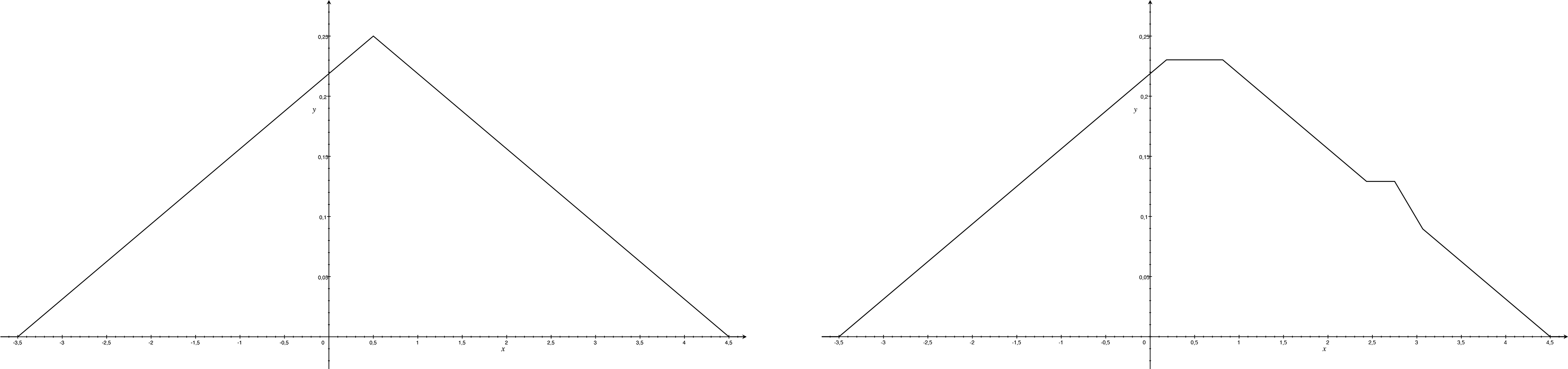
Figure 3: Functions $p_{0}$ and $p_{1,n}$ for $t=0.5$, $\beta=0.5$ and $n=10$

$(i)-(iii)$ Easy calculations show that both $p_{0}$ and $p_{1,n}$ are probability densities, which are bounded from below by $M=1/8$ on $B(t,2)$.

$(iv)$ We now verify that $p_{0|(-\varepsilon,1+\varepsilon)},\,p_{1,n|(-\varepsilon,1+\varepsilon)}\in\mathcal{H}_{(-\varepsilon,1+\varepsilon)}(1,L)$ for some Lipschitz constant $L>0$. Note again that for any $0<\varepsilon<1$ and any $t\in[0,1]$, the inclusion $(-\varepsilon,1+\varepsilon)\subset B(t,2)$ holds. Thus,

$$\sup_{\begin{subarray}{c}x,y\in(-\varepsilon,1+\varepsilon)\\ x\neq y\end{subarray}}\frac{|p_{0}(x)-p_{0}(y)|}{|x-y|}=\frac{1}{16}\cdot\sup_{\begin{subarray}{c}x,y\in(-\varepsilon,1+\varepsilon)\\ x\neq y\end{subarray}}\frac{||x-t|-|y-t||}{|x-y|}\leq\frac{1}{16}.$$

Since $p_{0}$ has maximal value $1/4$, we obtain that

$$p_{0|(-\varepsilon,1+\varepsilon)}\in\mathcal{H}_{(-\varepsilon,1+\varepsilon)}\left(1,\frac{5}{16}\right).$$

For the same reasons as before, we also obtain

$$p_{1,n|(-\varepsilon,1+\varepsilon)}\in\mathcal{H}_{(-\varepsilon,1+\varepsilon)}\left(1,\frac{5}{16}\right).$$

$(v)$ Finally, we address the verification of Assumption 3.1 for the hypotheses $p_{0}$ and $p_{1,n}$. Again, for any $t^{\prime}\in[0,1]$ and any $h\in\mathcal{G}_{\infty}$ the inclusion $B(t^{\prime},2h)\subset B(t,2)$ holds, and we distinguish between several combinations of pairs $(t^{\prime},h)$ with $t^{\prime}\in[0,1]$ and $h\in\mathcal{G}_{\infty}$. We start with $p_{0}$.

$(v.1)$ If $t\notin B(t^{\prime},h)$, it holds that $\|p\|_{\beta,B(t^{\prime},h)}\leq 5/16$ for all $\beta>0$, such that (3.6) and (3.7) trivially hold for $u=h$ and $\beta=\infty$.

$(v.2)$ In case $t\in B(t^{\prime},h)$, the function $p_{0|B(t^{\prime},2h)}$ is not differentiable and

$$\|p_{0}\|_{1,B(t^{\prime},2h)}\leq 5/16.$$

Furthermore, $t\in B(t^{\prime},2h-g)$ for any $g\in\mathcal{G}_{\infty}$ with $g<2h/16$ and thus

$$\sup_{s\in B(t^{\prime},2h-g)}\left|(K_{R,g}\ast p)(s)-p(s)\right| \geq\left|(K_{R,g}\ast p)(t)-p(t)\right|=\frac{1}{32}g.$$

That is, (3.6) and (3.7) are satisfied for $u=2h$ and $\beta=1$ for sufficiently large $n\geq n_{0}$.

The density $p_{1,n}$ can be treated in a similar way. It is constant on the interval $B(t,g_{\beta,n})$. If $B(t^{\prime},h)$ does not intersect with $\{t-g_{\beta,n},t+g_{\beta,n}\}$, Assumption 3.1 is satisfied for $u=h$ and $\beta=\infty$. If the two sets intersect, $t-g_{\beta,n}$ or $t+g_{\beta,n}$ is contained in $B(t^{\prime},2h-g)$ for any $g\in\mathcal{G}_{\infty}$ with $g<2h/16$, and we proceed as before.

Again, combining $(i)-(v)$, it follows that $p_{0}$ and $p_{1,n}$ are contained in the class $\mathscr{P}_{k}$ with $p_{0|(-\varepsilon,1+\varepsilon)},p_{1,n|(-\varepsilon,1+\varepsilon)}\in\mathcal{H}_{(-\varepsilon,1+\varepsilon)}(1,L)$ for sufficiently large $k\geq k_{0}$ and some universal constant $L>0$. The absolute distance of the two hypotheses in $t$ equals

$$|p_{0}(t)-p_{1,n}(t)| =\frac{1}{16}g_{1,n}.$$

To bound the Kullback-Leibler divergence between the associated product probability measures $\mathbb{P}_{0}^{\otimes n}$ and $\mathbb{P}_{1,n}^{\otimes n}$, we derive as before

$$K(\mathbb{P}_{1,n}^{\otimes n},\mathbb{P}_{0}^{\otimes n}) \leq n\int\frac{\left(q_{t+\frac{9}{4},n}(x)-q_{t,n}(x)\right)^{2}}{p_{0}(x)}\mathbbm{1}\left\{p_{0}(x)>0\right\}\mathop{\mathrm{\mathstrut d}}\nolimits\!x$$

$$\leq 16n\int\left(q_{t+\frac{9}{4},n}(x)-q_{t,n}(x)\right)^{2}\mathop{\mathrm{\mathstrut d}}\nolimits\!x$$

$$=32n\int q_{0,n}(x)^{2}\mathop{\mathrm{\mathstrut d}}\nolimits\!x$$

$$=\frac{1}{12},$$

using $p_{0}(t+5/2)>1/16$. Using Theorem 2.2 in Tsybakov (2009) again,

$$\inf_{T_{n}}\sup_{\begin{subarray}{c}p\in\mathscr{P}_{k}:\\ p_{|(-\varepsilon,1+\varepsilon)}\in\mathcal{H}_{(-\varepsilon,1+\varepsilon)}(1,L^{*})\end{subarray}}\mathbb{P}_{p}^{\otimes n}\left(n^{\frac{1}{3}}\left|T_{n}(t)-p(t)\right|\geq\frac{1}{32}\right)$$

$$\hskip 142.26378pt\geq\max\left\{\frac{1}{4}\exp(-1/12),\,\frac{1-\sqrt{1/24}}{2}\right\}>0.$$

Proof 5.6 (Proof of Proposition 3.4).

Define

$$\tilde{\mathscr{R}}=\bigcup_{n\in\mathbb{N}}\tilde{\mathscr{R}}_{n}$$

with

$$\tilde{\mathscr{R}}_{n}= \Bigg{\{}p\in\mathcal{H}_{(-\varepsilon,1+\varepsilon)}(\beta_{*}):\forall\,t\in[0,1]\ \forall\,h\in\mathcal{G}_{\infty}\ \exists\,\beta\in[\beta_{*},\beta^{*}]\text{ with }$$

$$\hskip 14.22636ptp_{|B(t,h)}\in\mathcal{H}_{B(t,h)}(\beta)\text{and }\|(K_{R,g}\ast p)-p\|_{B(t,h-g)}\geq\frac{g^{\beta}}{\log n}$$

$$\hskip 142.26378pt\text{ for all }g\in\mathcal{G}_{\infty}\text{ with }g\leq h/8\Bigg{\}}.$$

Furthermore, let

$$E_{n}(\beta)= \Bigg{\{}p\in\mathcal{H}_{(-\varepsilon,1+\varepsilon)}(\beta):\|(K_{R,g}\ast p)-p\|_{B(t,h-g)}\geq\frac{2}{\log n}g^{\beta}\text{ for all }t\in[0,1],$$

$$\hskip 99.58464pt\text{ for all }\,\,h\in\mathcal{G}_{\infty}\text{, and for all }g\in\mathcal{G}_{\infty}\text{ with }g\leq h/8\Bigg{\}}.$$

Note that Lemma 3.5 shows that $E_{n}(\beta)$ is non-empty as soon as

$$\frac{2}{\log n}\leq 1-\frac{4}{\pi}.$$

Note additionally that $E_{n}(\beta)\subset\tilde{\mathscr{R}}_{n}$ for any $\beta\in[\beta_{*},\beta^{*}]$, and

$$\bigcup_{n\in\mathbb{N}}E_{n}(\beta)\subset\tilde{\mathscr{R}}.$$

With

$$A_{n}(\beta)=\left\{\tilde{f}\in\mathcal{H}_{(-1,2)}(\beta):\|\tilde{f}-f\|_{\beta,(-\varepsilon,1+\varepsilon)}<\frac{\|K_{R}\|_{1}^{-1}}{\log n}\text{ for some }f\in E_{n}(\beta)\right\},$$

we get for any $\tilde{f}\in A_{n}(\beta)$ and a corresponding $f\in E_{n}(\beta)$ with

$$\|\check{f}\|_{\beta,(-\varepsilon,1+\varepsilon)}<\|K_{R}\|_{1}^{-1}\frac{1}{\log n}$$

and $\check{f}=\tilde{f}-f$, the lower bound

$$\Big{\|}(K_{R,g}\ast\tilde{f})-\tilde{f}\Big{\|}_{B(t,h-g)}$$

$$\geq\Big{\|}(K_{R,g}\ast f)-f\Big{\|}_{B(t,h-g)}-\Big{\|}\check{f}-(K_{R,g}\ast\check{f})\Big{\|}_{B(t,h-g)}$$

$$=\frac{2}{\log n}g^{\beta}-\sup_{s\in B(t,h-g)}\left|\int K_{R}(x)\left\{\check{f}(s+gx)-\check{f}(s)\right\}\mathop{\mathrm{\mathstrut d}}\nolimits\!x\right|$$

$$\geq\frac{2}{\log n}g^{\beta}-g^{\beta}\cdot\int|K_{R}(x)|\sup_{s\in B(t,h-g)}\sup_{\begin{subarray}{c}s^{\prime}\in B(s,g)\\ s^{\prime}\neq s\end{subarray}}\frac{\left|\check{f}(s^{\prime})-\check{f}(s)\right|}{|s-s^{\prime}|^{\beta}}\mathop{\mathrm{\mathstrut d}}\nolimits\!x$$

$$\geq\frac{2}{\log n}g^{\beta}-g^{\beta}\cdot\|K_{R}\|_{1}\cdot\|\check{f}\|_{\beta,(-\varepsilon,1+\varepsilon)}$$

$$\geq\frac{1}{\log n}g^{\beta}$$

for all $g,h\in\mathcal{G}_{\infty}$ with $g\leq h/8$ and for all $t\in[0,1]$, and therefore

$$A=\bigcup_{n\in\mathbb{N}}A_{n}(\beta)\subset\tilde{\mathscr{R}}.$$

Clearly, $A_{n}(\beta)$ is open in $\mathcal{H}_{(-\varepsilon,1+\varepsilon)}(\beta)$. Hence, the same holds true for $A$. Next, we verify that $A$ is dense in $\mathcal{H}_{(-\varepsilon,1+\varepsilon)}(\beta)$. Let $p\in\mathcal{H}_{(-\varepsilon,1+\varepsilon)}(\beta)$ and let $\delta>0$. We now show that there exists some function $\tilde{p}_{\delta}\in A$ with $\|p-\tilde{p}_{\delta}\|_{\beta,(-\varepsilon,1+\varepsilon)}\leq\delta$. For the construction of the function $\tilde{p}_{\delta}$, set the grid points

$$t_{j,1}(k)=(4j+1)2^{-k},\quad t_{j,2}(k)=(4j+3)2^{-k}$$

for $j\in\{-2^{k-2},-2^{k-2}+1,\ldots,2^{k-1}-1\}$ and $k\geq 2$. The function $\tilde{p}_{\delta}$ shall be defined as the limit of a recursively constructed sequence. The idea is to recursively add appropriately rescaled sine waves at those locations where the bias condition is violated. Let $p_{1,\delta}=p$, and denote

$$J_{k}=\bigg{\{}j\in\{-2^{k-2},\ldots,2^{k-1}-1\}: \max_{i=1,2}\Big{|}(K_{R,2^{-k}}\ast p_{k-1,\delta})(t_{j,i}(k))-p_{k-1,\delta}(t_{j,i}(k))\Big{|}$$

$$\hskip 85.35826pt<\frac{1}{2}c_{9}\,\delta\left(1-\frac{2}{\pi}\right)2^{-k\beta}\bigg{\}}$$

for $k\geq 2$, where

$$c_{9}=c_{9}(\beta)=\left(\frac{3\pi}{2}\cdot\frac{1}{1-2^{\beta-1}}+\frac{7}{1-2^{-\beta}}\right)^{-1}.$$

For any $k\geq 2$ set

$$p_{k,\delta}(x)=p_{k-1,\delta}(x)+c_{9}\,\delta\sum_{j\in J_{k}}S_{k,\beta,j}(x)$$

with functions

$$S_{k,\beta,j}(x)=2^{-k\beta}\sin\left(2^{k-1}\pi x\right)\mathbbm{1}\left\{|(4j+2)2^{-k}-x|\leq 2^{-k+1}\right\}$$

exemplified in Figure 4. That is,

$$p_{k,\delta}(x)=p(x)+c_{9}\,\delta\sum_{l=2}^{k}\sum_{j\in J_{l}}S_{l,\beta,j}(x),$$

and we define $\tilde{p}_{\delta}$ as the limit

$$\tilde{p}_{\delta}(x) =p(x)+c_{9}\,\delta\sum_{l=2}^{\infty}\sum_{j\in J_{l}}S_{l,\beta,j}(x)$$

$$=p_{k,\delta}(x)+c_{9}\,\delta\sum_{l=k+1}^{\infty}\sum_{j\in J_{l}}S_{l,\beta,j}(x).$$

The function $\tilde{p}_{\delta}$ is well-defined as the series on the right-hand side converges: for fixed $l\in\mathbb{N}$, the indicator functions

$$\mathbbm{1}\left\{|(4j+2)2^{-k}-x|\leq 2^{-k+1}\right\},\quad j\in\{-2^{l-2},-2^{l-2}+1,\ldots,2^{l-1}-1\}$$

have disjoint supports, such that

$$\bigg{\|}\sum_{j\in J_{l}}S_{l,\beta,j}\bigg{\|}_{(-\varepsilon,1+\varepsilon)}\leq 2^{-l\beta}.$$

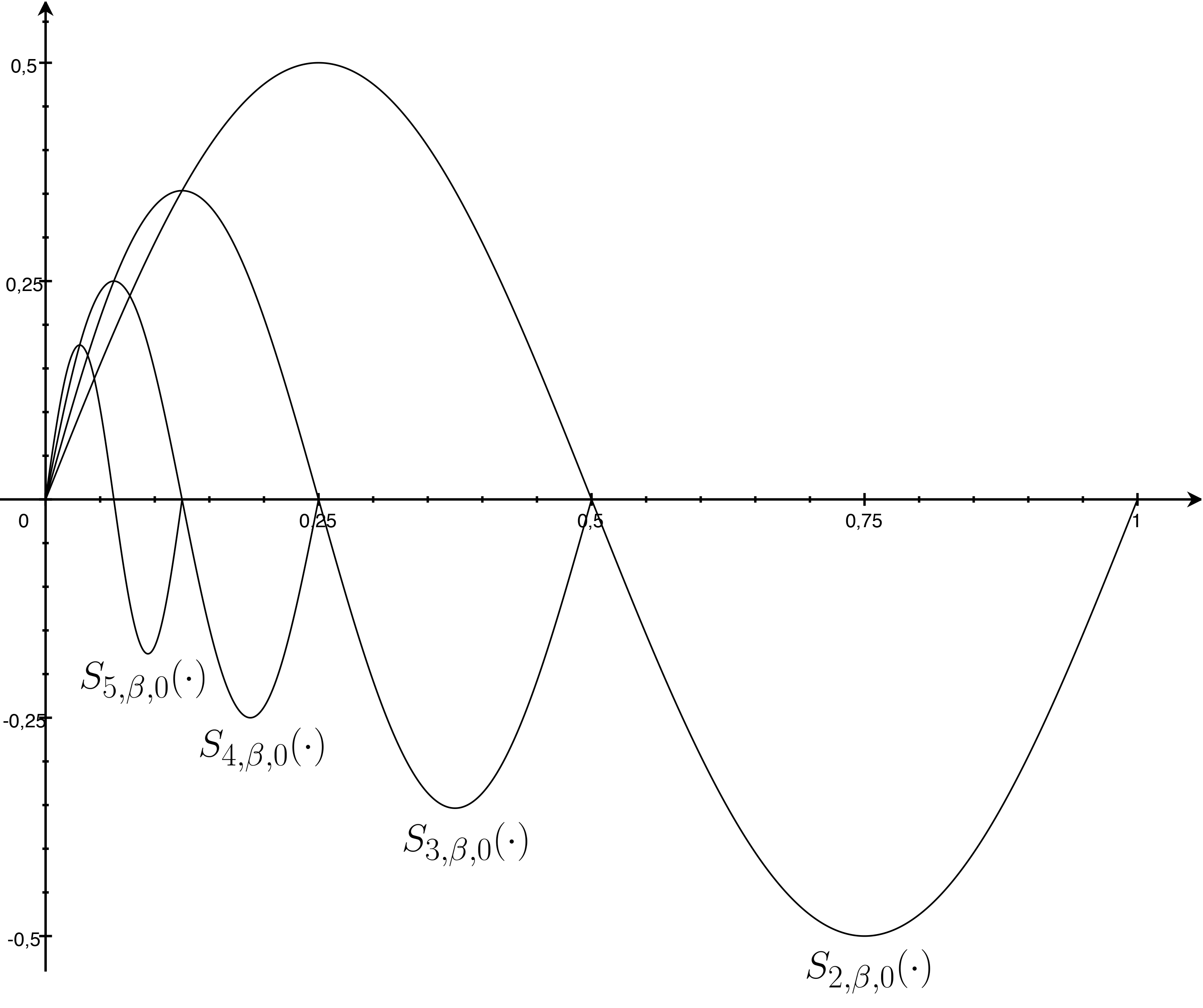
Figure 4: Functions $S_{k,\beta,0}$ for $k=2,\ldots,5$ and $\beta=0.5$

It remains to verify that $\tilde{p}_{\delta}\in\bigcup_{n\in\mathbb{N}}E_{n}(\beta)\subset A$ and also $\|p-\tilde{p}_{\delta}\|_{\beta,(-\varepsilon,1+\varepsilon)}\leq\delta$. As concerns the inequality $\|p-\tilde{p}_{\delta}\|_{\beta,(-\varepsilon,1+\varepsilon)}\leq\delta$, it remains to show that

$$\left\|\sum_{l=2}^{\infty}\sum_{j\in J_{l}}S_{l,\beta,j}\right\|_{\beta,(-\varepsilon,1+\varepsilon)}\leq\frac{1}{c_{9}}.$$

For $s,t\in(-\varepsilon,1+\varepsilon)$ with $|s-t|\leq 1$, we obtain

$$\left|\sum_{l=2}^{\infty}\sum_{j\in J_{l}}S_{l,\beta,j}(s)-\sum_{l=2}^{\infty}\sum_{j\in J_{l}}S_{l,\beta,j}(t)\right|$$

$$\hskip 28.45274pt\leq\sum_{l=2}^{\infty}2^{-l\beta}\bigg{|}\sin(2^{l-1}\pi s)\sum_{j\in J_{l}}\mathbbm{1}\{|(4j+2)2^{-l}-s|\leq 2^{-l+1}\}$$ (5.4)

$$\hskip 99.58464pt-\sin(2^{l-1}\pi t)\sum_{j\in J_{l}}\mathbbm{1}\{|(4j+2)2^{-l}-t|\leq 2^{-l+1}\}\bigg{|}.$$

Choose now $k^{\prime}\in\mathbb{N}$ maximal, such that both

$$(4j+2)2^{-k^{\prime}}-2^{-k^{\prime}+1}\leq s\leq(4j+2)2^{-k^{\prime}}+2^{-k^{\prime}+1}$$

and

$$(4j+2)2^{-k^{\prime}}-2^{-k^{\prime}+1}\leq t\leq(4j+2)2^{-k^{\prime}}+2^{-k^{\prime}+1}$$

for some $j\in\{-2^{k^{\prime}-2},\ldots,2^{k^{\prime}-1}-1\}$. For $2\leq l\leq k^{\prime}$, we have

$$\bigg{|}\sin(2^{l-1}\pi s)\sum_{j\in J_{l}}\mathbbm{1}\{|(4j+2)2^{-l}-s|\leq 2^{-l+1}\}$$

$$\hskip 128.0374pt-\sin(2^{l-1}\pi t)\sum_{j\in J_{l}}\mathbbm{1}\{|(4j+2)2^{-l}-t|\leq 2^{-l+1}\}\bigg{|}$$

$$\qquad\leq\bigg{|}\sin(2^{l-1}\pi s)-\sin(2^{l-1}\pi t)\bigg{|}$$

$$\qquad\leq\min\left\{2^{l-1}\pi|s-t|,2\right\}$$ (5.5)

by the mean value theorem. For $l\geq k^{\prime}+1$,

$$\bigg{|}\sin(2^{l-1}\pi s)\sum_{j\in J_{l}}\mathbbm{1}\{|(4j+2)2^{-l}-s|\leq 2^{-l+1}\}$$

$$\hskip 128.0374pt-\sin(2^{l-1}\pi t)\sum_{j\in J_{l}}\mathbbm{1}\{|(4j+2)2^{-l}-t|\leq 2^{-l+1}\}\bigg{|}$$

$$\leq\max\Bigg{\{}\bigg{|}\sin(2^{l-1}\pi s)\bigg{|},\bigg{|}\sin(2^{l-1}\pi t)\bigg{|}\Bigg{\}}.$$

Furthermore, due to the choice of $k^{\prime}$, there exists some $z\in[s,t]$ with

$$\sin(2^{l-1}\pi z)=0$$

for all $l\geq k^{\prime}+1$. Thus, for any $l\geq k^{\prime}+1$, by the mean value theorem,

$$\bigg{|}\sin(2^{l-1}\pi s)\bigg{|} =\bigg{|}\sin(2^{l-1}\pi s)-\sin(2^{l-1}\pi z)\bigg{|}$$

$$\leq\min\left\{2^{l-1}\pi|s-z|,1\right\}$$

$$\leq\min\left\{2^{l-1}\pi|s-t|,1\right\}.$$

Analogously, we obtain

$$\bigg{|}\sin(2^{l-1}\pi t)\bigg{|}\leq\min\left\{2^{l-1}\pi|s-t|,1\right\}.$$

Consequently, together with inequality (5.6) and (5.6),

$$\left|\sum_{l=2}^{\infty}\sum_{j\in J_{l}}S_{l,\beta,j}(s)-\sum_{l=2}^{\infty}\sum_{j\in J_{l}}S_{l,\beta,j}(t)\right|\leq\sum_{l=2}^{\infty}2^{-l\beta}\min\left\{2^{l-1}\pi|s-t|,\,2\right\}.$$

Choose now $k\in\mathbb{N}\cup\{0\}$, such that $2^{-(k+1)}<|s-t|\leq 2^{-k}$. If $k\leq 1$,

$$\sum_{l=2}^{\infty}2^{-l\beta}\min\left\{2^{l-1}\pi|s-t|,\,2\right\}\leq 2\frac{2^{-2\beta}}{1-2^{-\beta}}\leq\frac{2}{1-2^{-\beta}}|s-t|^{\beta}.$$

If $k\geq 2$, we decompose

$$\sum_{l=2}^{\infty}2^{-l\beta}\min\left\{2^{l-1}\pi|s-t|,\,2\right\} \leq\frac{\pi}{2}|s-t|\,\sum_{l=0}^{k}2^{l(1-\beta)}+2\sum_{l=k+1}^{\infty}2^{-l\beta}$$

$$=\frac{\pi}{2}|s-t|\,\frac{2^{k(1-\beta)}-2^{\beta-1}}{1-2^{\beta-1}}+2\cdot\frac{2^{-(k+1)\beta}}{1-2^{-\beta}}$$

$$\leq|s-t|^{\beta}\cdot\left(\frac{\pi}{2}\cdot\frac{1}{1-2^{\beta-1}}+\frac{2}{1-2^{-\beta}}\right).$$

Since furthermore

$$\left\|\sum_{l=2}^{\infty}\sum_{j\in J_{l}}S_{l,\beta,j}\right\|_{\sup}\leq\frac{1}{1-2^{-\beta}},$$

we have

$$\left\|\sum_{l=2}^{\infty}\sum_{j\in J_{l}}S_{l,\beta,j}\right\|_{\beta,(-\varepsilon,1+\varepsilon)}\leq 3\left(\frac{\pi}{2}\cdot\frac{1}{1-2^{\beta-1}}+\frac{2}{1-2^{-\beta}}\right)+\frac{1}{1-2^{-\beta}}=\frac{1}{c_{9}}$$

and finally $\|p-\tilde{p}_{\varepsilon}\|_{\beta,(-\varepsilon,1+\varepsilon)}\leq\delta$. In particular $\tilde{p}_{\delta}\in\mathcal{H}_{(-\varepsilon,1+\varepsilon)}(\beta)$.

We now show that the function $\tilde{p}_{\delta}$ is contained in $\bigcup_{n\in\mathbb{N}}E_{n}(\beta)\subset A$. For any bandwidths $g,h\in\mathcal{G}_{\infty}$ with $g\leq h/8$, it holds that $h-g\geq 4g$. Thus, for any $g=2^{-k}$ with $k\geq 2$ and for any $t\in(-\varepsilon,1+\varepsilon)$, there exists some $j=j(t,h,g)\in\{-2^{k-2},\ldots,2^{k-1}-1\}$ such that both $t_{j,1}(k)$ and $t_{j,2}(k)$ are contained in $B(t,h-g)$, which implies

$$\sup_{s\in B(t,h-g)}\left|(K_{R,g}\ast\tilde{p}_{\delta})(s)-\tilde{p}_{\delta}(s)\right|\geq\max_{i=1,2}\left|(K_{R,g}\ast\tilde{p}_{\delta})(t_{j,i}(k))-\tilde{p}_{\delta}(t_{j,i}(k))\right|.$$ (5.6)

By linearity of the convolution and the theorem of dominated convergence,

$$(K_{R,g}\ast\tilde{p}_{\delta})(t_{j,i}(k))-\tilde{p}_{\delta}(t_{j,i}(k))$$

$$\qquad=(K_{R,g}\ast p_{k,\delta})(t_{j,i}(k))-p_{k,\delta}(t_{j,i}(k))$$

$$\qquad\qquad+c_{9}\,\delta\sum_{l=k+1}^{\infty}\sum_{j\in J_{l}}\Big{(}(K_{R,g}\ast S_{l,\beta,j})(t_{j,i}(k))-S_{l,\beta,j}(t_{j,i}(k))\Big{)}.$$ (5.7)

We analyze the convolution $K_{R,g}\ast S_{l,\beta,j}$ for $l\geq k+1$. Here,

$$\sin\left(2^{l-1}\pi\,t_{j,1}(k)\right)=\sin\left(2^{l-k-1}\pi\,(4j+1)\right)=0$$

and

$$\sin\left(2^{l-1}\pi\,t_{j,2}(k)\right)=\sin\left(2^{l-k-1}\pi\,(4j+3)\right)=0.$$

Hence,

$$\sum_{j\in J_{l}}S_{l,\beta,j}(t_{j,i}(k))=0,\quad i=1,2$$

for any $l\geq k+1$. Furthermore,

$$(K_{R,g}\ast S_{l,\beta,j})(t_{j,i}(k)) =\frac{1}{2g}\int_{-g}^{g}S_{l,\beta,j}(t_{j,i}(k)-x)\mathop{\mathrm{\mathstrut d}}\nolimits\!x$$

$$=\frac{1}{2g}\int_{t_{j,i}(k)-g}^{t_{j,i}(k)+g}S_{l,\beta,j}(x)\mathop{\mathrm{\mathstrut d}}\nolimits\!x,\quad i=1,2.$$

Due to the identities

$$(4j+2)2^{-k}-2^{-k+1} =t_{j,1}(k)-g$$

$$(4j+2)2^{-k}+2^{-k+1} =t_{j,2}(k)+g,$$

we have either

$$\left[(4j+2)2^{-l}-2^{-l+1},(4j+2)2^{-l}+2^{-l+1}\right]\subset\left[t_{j,1}(k)-g,t_{j,2}(k)+g\right]$$

or

$$\left[(4j+2)2^{-l}-2^{-l+1},(4j+2)2^{-l}+2^{-l+1}\right]\cap\left[t_{j,1}(k)-g,t_{j,2}(k)+g\right]=\emptyset$$

for any $l\geq k+1$. Therefore, for $i=1,2$,

$$\sum_{j\in J_{l}}(K_{R,g}\ast S_{l,\beta,j})(t_{j,i}(k))$$

$$\quad=\sum_{j\in J_{l}}\frac{1}{2g}\int_{t_{j,i}(k)-g}^{t_{j,i}(k)+g}2^{-l\beta}\sin\left(2^{l-1}\pi x\right)\mathbbm{1}\left\{|(4j+2)2^{-l}-x|\leq 2^{-l+1}\right\}\mathop{\mathrm{\mathstrut d}}\nolimits\!x$$

$$\quad=0$$

such that equation (5.6) then simplifies to

$$(K_{R,g}\ast\tilde{p}_{\delta})(t_{j,i}(k))-\tilde{p}_{\delta}(t_{j,i}(k)) =(K_{R,g}\ast p_{k,\delta})(t_{j,i}(k))-p_{k,\delta}(t_{j,i}(k)),\quad i=1,2.$$

Together with (5.6), we obtain

$$\sup_{s\in B(t,h-g)}\left|(K_{R,g}\ast\tilde{p}_{\delta})(s)-\tilde{p}_{\delta}(s)\right|\geq\max_{i=1,2}\left|(K_{R,g}\ast p_{k,\delta})(t_{j,i}(k))-p_{k,\delta}(t_{j,i}(k))\right|$$

for some $j\in\{-2^{k-2},-2^{k-2}+1,\ldots,2^{k-2}-1\}$. If $j\notin J_{k}$, then

$$\max_{i=1,2}\left|(K_{R,g}\ast p_{k,\delta})(t_{j,i}(k))-p_{k,\delta}(t_{j,i}(k))\right|$$

$$\hskip 56.9055pt=\max_{i=1,2}\left|(K_{R,g}\ast p_{k-1,\delta})(t_{j,i}(k))-p_{k-1,\delta}(t_{j,i}(k))\right|$$

$$\hskip 56.9055pt\geq\frac{1}{2}c_{9}\,\delta\left(1-\frac{2}{\pi}\right)g^{\beta}.$$

If $j\in J_{k}$, then

$$\max_{i=1,2}\left|(K_{R,g}\ast p_{k,\delta})(t_{j,i}(k))-p_{k,\delta}(t_{j,i}(k))\right|$$

$$\quad\geq c_{9}\,\delta\max_{i=1,2}\left|(K_{R,g}\ast S_{k,\beta,j})(t_{j,i}(k))-S_{k,\beta,j}(t_{j,i}(k))\right|$$

$$\qquad-\max_{i=1,2}\left|(K_{R,g}\ast p_{k-1,\delta})(t_{j,i}(k))-p_{k-1,\delta}(t_{j,i}(k))\right|$$

$$\quad\geq c_{9}\,\delta\max_{i=1,2}\left|(K_{R,g}\ast S_{k,\beta,j})(t_{j,i}(k))-S_{k,\beta,j}(t_{j,i}(k))\right|-\frac{1}{2}c_{9}\,\delta\left(1-\frac{2}{\pi}\right)g^{\beta}.$$

Similar as above we obtain

$$(K_{R,g}\ast S_{k,\beta,j})(t_{j,1}(k))-S_{k,\beta,j}(t_{j,1}(k))$$

$$\hskip 56.9055pt=\frac{1}{2g}\int_{t_{j,1}(k)-g}^{t_{j,1}(k)+g}2^{-k\beta}\sin\left(2^{k-1}\pi x\right)\mathop{\mathrm{\mathstrut d}}\nolimits\!x-2^{-k\beta}$$

$$\hskip 56.9055pt=\frac{1}{2g}2^{-k\beta}\int_{0}^{2^{-k+1}}\sin\left(2^{k-1}\pi x\right)\mathop{\mathrm{\mathstrut d}}\nolimits\!x-2^{-k\beta}$$

$$\hskip 56.9055pt=g^{\beta}\left(\frac{2}{\pi}-1\right)$$

as well as

$$(K_{R,g}\ast S_{k,\beta,j})(t_{j,2}(k))-S_{k,\beta,j}(t_{j,2}(k))=g^{\beta}\left(1-\frac{2}{\pi}\right),$$

such that

$$\max_{i=1,2}\left|(K_{R,g}\ast p_{k,\delta})(t_{j,i}(k))-p_{k,\delta}(t_{j,i}(k))\right| \geq\frac{1}{2}c_{9}\,\delta\left(1-\frac{2}{\pi}\right)g^{\beta}.$$

Combining the two cases finally gives

$$\sup_{s\in B(t,h-g)}\left|(K_{R,g}\ast\tilde{p}_{\delta})(s)-\tilde{p}_{\delta}(s)\right|\geq\frac{1}{2}c_{9}\,\delta\left(1-\frac{2}{\pi}\right)g^{\beta}.$$

In particular, $\tilde{p}_{\delta}\in E_{n}(\beta)$ for sufficiently large $n\geq n_{0}(\beta,\delta)$, and thus $\tilde{p}_{\delta}\in A$.

Since $A$ is open and dense in the class $\mathcal{H}_{(-\varepsilon,1+\varepsilon)}(\beta)$ and $A\subset\tilde{\mathscr{R}}$, the complement $\mathcal{H}_{(-\varepsilon,1+\varepsilon)}(\beta)\setminus\tilde{\mathscr{R}}$ is nowhere dense in $H_{(-\varepsilon,1+\varepsilon)}(\beta)$. Thus, because of

$$\mathcal{H}_{(-\varepsilon,1+\varepsilon)}(\beta)_{|B(t,h)}=\mathcal{H}_{B(t,h)}(\beta),$$

and the fact that for any $x\in\mathcal{H}_{(-\varepsilon,1+\varepsilon)}(\beta)$ and any $z^{\prime}\in\mathcal{H}_{B(t,h)}(\beta)$ with

$$\|x_{|B(t,h)}-z^{\prime}\|_{\beta,B(t,h)}<\delta$$

there exists an extension $z\in\mathcal{H}_{(-\varepsilon,1+\varepsilon)}(\beta)$ of $z^{\prime}$ with

$$\|x-z\|_{\beta,(-\varepsilon,1+\varepsilon)}<\delta,$$

the set $\mathcal{H}_{B(t,h)}(\beta)\setminus\tilde{\mathscr{R}}_{|B(t,h)}$ is nowhere dense in $\mathcal{H}_{B(t,h)}(\beta)$. Since the property ”nowhere dense” is stable when passing over to intersections and the corresponding relative topology, we conclude that

$$\mathcal{P}_{B(t,h)}(\beta,L^{*})\setminus\mathscr{R}_{|B(t,h)}$$

is nowhere dense in $\mathcal{P}_{B(t,h)}(\beta,L^{*})$ with respect to $\|\cdot\|_{\beta,B(t,h)}$.

Proof 5.7 (Proof of Lemma 3.5).

As it has been proven in Hardy (1916) the Weierstraß function $W_{\beta}$ is $\beta$-Hölder continuous everywhere. For the sake of completeness, we state the proof here. Because the Weierstraß function is $2$-periodic, it suffices to consider points $s,t\in\mathbb{R}$ with $|s-t|\leq 1$. Note first that

$$|W_{\beta}(s)-W_{\beta}(t)| \leq 2\sum_{n=0}^{\infty}2^{-n\beta}\left|\sin\left(\frac{1}{2}2^{n}\pi(s+t)\right)\right|\cdot\left|\sin\left(\frac{1}{2}2^{n}\pi(s-t)\right)\right|$$

$$\leq 2\sum_{n=0}^{\infty}2^{-n\beta}\left|\sin\left(\frac{1}{2}2^{n}\pi(s-t)\right)\right|.$$

Choose $k\in\mathbb{N}\cup\{0\}$ such that $2^{-(k+1)}<|s-t|\leq 2^{-k}$. For all summands with index $n\leq k$, use the inequality $|\sin(x)|\leq|x|$ and for all summands with index $n>k$ use $|\sin(x)|\leq 1$, such that

$$|W_{\beta}(s)-W_{\beta}(t)| \leq 2\sum_{n=0}^{k}2^{-n\beta}\left|\frac{1}{2}2^{n}\pi(s-t)\right|+2\sum_{n=k+1}^{\infty}2^{-n\beta}$$

$$=\pi\left|s-t\right|\sum_{n=0}^{k}2^{n(1-\beta)}+2\sum_{n=k+1}^{\infty}2^{-n\beta}.$$

Note that,

$$\sum_{n=0}^{k}2^{n(1-\beta)}=\frac{2^{(k+1)(1-\beta)}-1}{2^{1-\beta}-1}=\frac{2^{k(1-\beta)}-2^{\beta-1}}{1-2^{\beta-1}}\leq\frac{2^{k(1-\beta)}}{1-2^{\beta-1}},$$

and, as $2^{-\beta}<1$,

$$\sum_{n=k+1}^{\infty}2^{-n\beta} =\frac{2^{-(k+1)\beta}}{1-2^{-\beta}}.$$

Consequently, we have

$$\begin{split}|W_{\beta}(s)-W_{\beta}(t)|&\leq\pi\left|s-t\right|\frac{2^{k(1-\beta)}}{1-2^{\beta-1}}+2\frac{2^{-(k+1)\beta}}{1-2^{-\beta}}\\ &\leq\left|s-t\right|^{\beta}\left(\frac{\pi}{1-2^{\beta-1}}+\frac{2}{1-2^{-\beta}}\right).\end{split}$$

Furthermore

$$\|W_{\beta}\|_{\sup}\leq\sum_{n=0}^{\infty}2^{-n\beta}=\frac{1}{1-2^{-\beta}},$$

so that for any interval $U\subset\mathbb{R}$,

$$\|W_{\beta}\|_{\beta,U}\leq\frac{\pi}{1-2^{\beta-1}}+\frac{3}{1-2^{-\beta}}.$$

We now turn to the proof of bias lower bound condition. For any $0<\beta\leq 1$, for any $h\in\mathcal{G}_{\infty}$, for any $g=2^{-k}\in\mathcal{G}_{\infty}$ with $g\leq h/2$, and for any $t\in\mathbb{R}$, there exists some $s_{0}\in[t-(h-g),t+(h-g)]$ with $\cos\left(2^{k}\pi s_{0}\right)=1$, since the function $x\mapsto\cos(2^{k}\pi x)$ is $2^{1-k}$-periodic. Note that in this case also

$$\cos\left(2^{n}\pi s_{0}\right)=1\quad\text{ for all }n\geq k.$$ (5.8)

The following supremum is now lower bounded by

$$\sup_{s\in B(t,h-g)}\left|\int K_{R,g}(x-s)W_{\beta}(x)\mathop{\mathrm{\mathstrut d}}\nolimits\!x-W_{\beta}(s)\right|$$

$$\hskip 142.26378pt\geq\left|\int_{-1}^{1}K_{R}(x)W_{\beta}(s_{0}+gx)\mathop{\mathrm{\mathstrut d}}\nolimits\!x-W_{\beta}(s_{0})\right|.$$

As furthermore

$$\sup_{x\in\mathbb{R}}\left|K_{R}(x)2^{-n\beta}\cos\left(2^{n}\pi(s_{0}+gx)\right)\right|\leq\|K_{R}\|_{\sup}\cdot 2^{-n\beta}$$

and

$$\sum_{n=0}^{\infty}\|K_{R}\|_{\sup}\cdot 2^{-n\beta}=\frac{\|K_{R}\|_{\sup}}{1-2^{-\beta}}<\infty,$$

the dominated convergence theorem implies

$$\left|\int_{-1}^{1}K_{R}(x)W_{\beta}(s_{0}+gx)\mathop{\mathrm{\mathstrut d}}\nolimits\!x-W_{\beta}(s_{0})\right|=\left|\sum_{n=0}^{\infty}2^{-n\beta}I_{n}(s_{0},g)\right|$$

with

$$I_{n}(s_{0},g)=\int_{-1}^{1}K_{R}(x)\cos\left(2^{n}\pi(s_{0}+gx)\right)\mathop{\mathrm{\mathstrut d}}\nolimits\!x-\cos\left(2^{n}\pi s_{0}\right).$$

Recalling (5.8), it holds for any index $n\geq k$

$$I_{n}(s_{0},g) =\frac{1}{2}\cdot\frac{\sin(2^{n}\pi(s_{0}+g))-\sin(2^{n}\pi(s_{0}-g))}{2^{n}\pi g}-1$$

$$=\frac{\sin(2^{n}\pi g)}{2^{n}\pi g}-1$$

$$=-1.$$ (5.9)

Furthermore, for any index $0\leq n\leq k-1$ holds

$$I_{n}(s_{0},g) =\frac{1}{2}\cdot\frac{\sin(2^{n}\pi(s_{0}+g))-\sin(2^{n}\pi(s_{0}-g))}{2^{n}\pi g}-\cos\left(2^{n}\pi s_{0}\right)$$

$$=\cos(2^{n}\pi s_{0})\left(\frac{\sin(2^{n}\pi g)}{2^{n}\pi g}-1\right).$$ (5.10)

Using this representation, the inequality $\sin(x)\leq x$ for $x\geq 0$, and Lemma A.5, we obtain

$$2^{-n\beta}I_{n}(s_{0},g) \leq 2^{-n\beta}\left(1-\frac{\sin(2^{n}\pi g)}{2^{n}\pi g}\right)$$

$$\leq 2^{-n\beta}\cdot\frac{(2^{n}\pi g)^{2}}{6}$$

$$\leq 2^{-n\beta+2(n-k)+1}.$$

Since $k-n-1\geq 0$ and $\beta\leq 1$, this is in turn bounded by

$$2^{-n\beta}I_{n}(s_{0},g) \leq 2^{-(2k-n-2)\beta}\cdot 2^{2(n-k)+1+2(k-n-1)\beta}$$

$$\leq 2^{-(2k-n-2)\beta}\cdot 2^{2(n-k)+1+2(k-n-1)}$$

$$\leq 2^{-(2k-n-2)\beta}.$$ (5.11)

Taking together (5.7) and (5.7), we arrive at

$$\sum_{n=0}^{k-3}2^{-n\beta}I_{n}(s_{0},g)+\sum_{n=k+1}^{2k-2}2^{-n\beta}I_{n}(s_{0},g) \leq\sum_{n=0}^{k-3}2^{-(2k-n-2)\beta}-\sum_{n=k+1}^{2k-2}2^{-n\beta}=0.$$

Since by (5.7) also

$$\sum_{n=2k-1}^{\infty}2^{-n\beta}I_{n}(s_{0},g)=-\sum_{n=2k-1}^{\infty}2^{-n\beta}<0,$$

it remains to investigate

$$\sum_{n=k-2}^{k}2^{-n\beta}I_{n}(s_{0},g).$$

For this purpose, we distinguish between the three cases

$$(i)\quad \cos(2^{k-1}\pi s_{0})=\cos(2^{k-2}\pi s_{0})=1$$

$$(ii)\quad \cos(2^{k-1}\pi s_{0})=-1,\ \cos(2^{k-2}\pi s_{0})=0$$

$$(iii)\quad \cos(2^{k-1}\pi s_{0})=1,\ \cos(2^{k-2}\pi s_{0})=-1$$

and subsequently use the representation in (5.7). In case $(i)$, obviously

$$\sum_{n=k-2}^{k}2^{-n\beta}I_{n}(s_{0},g)\leq-2^{-k\beta}<0.$$

using $\sin(x)\leq x$ for $x\geq 0$ again. In case $(ii)$, we obtain for $\beta\leq 1$

$$\sum_{n=k-2}^{k}2^{-n\beta}I_{n}(s_{0},g) =2^{-k\beta}2^{\beta}\left(1-\frac{\sin(\pi/2)}{\pi/2}\right)-2^{-k\beta}\leq 2^{-k\beta}\left(1-\frac{4}{\pi}\right)<0.$$

Finally, in case $(iii)$, for $\beta\leq 1$,

$$\sum_{n=k-2}^{k}2^{-n\beta}I_{n}(s_{0},g)$$

$$\quad=2^{-(k-1)\beta}\left(\frac{\sin(\pi/2)}{\pi/2}-1\right)-2^{-(k-2)\beta}\left(\frac{\sin(\pi/4)}{\pi/4}-1\right)-2^{-k\beta}$$

$$\quad=2^{-(k-1)\beta}\left(\left(\frac{2}{\pi}-1\right)+2^{\beta}\left(1-\frac{\sin(\pi/4)}{\pi/4}\right)\right)-2^{-k\beta}$$

$$\quad<2^{-(k-1)\beta}\left(\frac{2}{\pi}+1-8\,\frac{\sin(\pi/4)}{\pi}\right)-2^{-k\beta}$$

$$\quad<-2^{-k\beta}$$

$$\quad<0.$$

That is,

$$\sup_{s\in B(t,h-g)}\left|\int K_{R,g}(x-s)W_{\beta}(x)\mathop{\mathrm{\mathstrut d}}\nolimits\!x-W_{\beta}(s)\right|$$

$$\hskip 56.9055pt\geq\left|\int_{-1}^{1}K_{R}(x)W_{\beta}(s_{0}+gx)\mathop{\mathrm{\mathstrut d}}\nolimits\!x-W_{\beta}(s_{0})\right|$$

$$\hskip 56.9055pt=-\sum_{n=0}^{\infty}2^{-n\beta}I_{n}(s_{0},g)$$

$$\hskip 56.9055pt\geq-\sum_{n=k-2}^{k}2^{-n\beta}I_{n}(s_{0},g)$$

$$\hskip 56.9055pt>\left(\frac{4}{\pi}-1\right)g^{\beta}.$$

Proof 5.8 (Proof of Theorem 3.1).

The proof is structured as follows. First, we show that the bias term is negligible. Then, we conduct several reduction steps to non-stationary Gaussian processes. We pass over to the supremum over a stationary Gaussian process by means of Slepian’s comparison inequality, and finally, we employ extreme value theory for its asymptotic distribution.

Step 1 (Negligibility of the bias)

Due to the discretization of the interval $[0,1]$ in the construction of the confidence band and due to the local variability of the confidence band’s width, the negligibility of the bias is not immediate. For any $t\in[0,1]$, there exists some $k_{t}\in T_{n}$ with $t\in I_{k_{t}}$. Hence,

$$\sqrt{\tilde{n}\hat{h}_{n}^{loc}(t)}\left|\mathbb{E}_{p}^{\chi_{1}}\hat{p}_{n}^{loc}(t,\hat{h}_{n}^{loc}(t))-p(t)\right|$$

$$\quad=\sqrt{\tilde{n}\hat{h}_{n,k_{t}}^{loc}}\Big{|}\mathbb{E}_{p}^{\chi_{1}}\hat{p}_{n}^{(1)}(k_{t}\delta_{n},\hat{h}_{n,k_{t}}^{loc})-p(t)\Big{|}$$

$$\quad\leq\sqrt{\tilde{n}\hat{h}_{n,k_{t}}^{loc}}\Big{|}\mathbb{E}_{p}^{\chi_{1}}\hat{p}_{n}^{(1)}(k_{t}\delta_{n},\hat{h}_{n,k_{t}}^{loc})-p(k_{t}\delta_{n})\Big{|}+\sqrt{\tilde{n}\hat{h}_{n,k_{t}}^{loc}}\Big{|}p(k_{t}\delta_{n})-p(t)\Big{|}.$$

Assume $\hat{j}_{n}(k\delta_{n})\geq k_{n}(k\delta_{n})=\bar{j}_{n}(k\delta_{n})-m_{n}$ for all $k\in T_{n}$, where $m_{n}$ is given in Proposition 4.1. Since $\delta_{n}\leq\frac{1}{8}h_{\beta_{*},n}$ for sufficiently large $n\geq n_{0}(\beta_{*},\varepsilon)$,

$$\hat{h}_{n,k_{t}}^{loc} =2^{m_{n}-u_{n}}\cdot\min\left\{2^{-\hat{j}_{n}((k_{t}-1)\delta_{n})-m_{n}},2^{-\hat{j}_{n}(k_{t}\delta_{n})-m_{n}}\right\}$$

$$\leq 2^{m_{n}-u_{n}}\cdot\min\left\{\bar{h}_{n}((k_{t}-1)\delta_{n}),\bar{h}_{n}(k_{t}\delta_{n})\right\}$$

$$\leq 3\cdot 2^{m_{n}-u_{n}}\cdot\bar{h}_{n}(t)$$

by Lemma 4.2. In particular, $\delta_{n}+\hat{h}_{n,k_{t}}^{loc}\leq 2^{-(\bar{j}_{n}(t)+1)}$ holds for sufficiently large $n\geq n_{0}(c_{1},\beta_{*})$, so that Assumption 3.1, Lemma 3.2, and Lemma 4.4 yield

$$\sup_{p\in\mathscr{P}_{n}}\sqrt{\tilde{n}\hat{h}_{n,k_{t}}^{loc}}\left|\mathbb{E}_{p}^{\chi_{1}}\hat{p}_{n}^{(1)}(k_{t}\delta_{n},\hat{h}_{n,k_{t}}^{loc})-p(k_{t}\delta_{n})\right|$$

$$\hskip 56.9055pt\leq\sup_{p\in\mathscr{P}_{n}}\sqrt{\tilde{n}\hat{h}_{n,k_{t}}^{loc}}\sup_{s\in B(t,\delta_{n})}\left|\mathbb{E}_{p}^{\chi_{1}}\hat{p}_{n}^{(1)}(s,\hat{h}_{n,k_{t}}^{loc})-p(s)\right|$$

$$\hskip 56.9055pt\leq\sup_{p\in\mathscr{P}_{n}}b_{2}\sqrt{\tilde{n}\hat{h}_{n,k_{t}}^{loc}}\left(\hat{h}_{n,k_{t}}^{loc}\right)^{\beta_{p}(B(t,2^{-\bar{j}_{n}(t)}))}$$

$$\hskip 56.9055pt\leq\sup_{p\in\mathscr{P}_{n}}b_{2}\sqrt{\tilde{n}\hat{h}_{n,k_{t}}^{loc}}\left(\hat{h}_{n,k_{t}}^{loc}\right)^{\beta_{p}(B(t,\bar{h}_{n}(t)))}$$

$$\hskip 56.9055pt\leq\sup_{p\in\mathscr{P}_{n}}b_{2}\left(3\cdot 2^{m_{n}-u_{n}}\right)^{\frac{2\beta_{*}+1}{2}}\sqrt{\tilde{n}\bar{h}_{n}(t)}\bar{h}_{n}(t)^{\beta_{n,p}(t)}$$

$$\hskip 56.9055pt\leq c_{10}\cdot(\log\tilde{n})^{-\frac{1}{4}c_{1}(2\beta_{*}+1)\log 2}$$ (5.12)

for some constant $c_{10}=b_{2}\cdot 3^{(2\beta_{*}+1)/2}$, on the event

$$\left\{\hat{j}_{n}(k\delta_{n})\geq k_{n}(k\delta_{n})\text{ for all }k\in T_{n}\right\}.$$

Now, we analyze the expression

$$\sqrt{\tilde{n}\hat{h}_{n,k_{t}}^{loc}}\Big{|}p(k_{t}\delta_{n})-p(t)\Big{|}.$$

For $t\in I_{k}$ and for $n\geq n_{0}$,

$$\delta_{n}^{\beta_{*}}\leq 2^{-j_{\min}}\left(\frac{\log\tilde{n}}{\tilde{n}}\right)^{\kappa_{1}\beta_{*}}\leq 2^{-j_{\min}}\left(\frac{\log\tilde{n}}{\tilde{n}}\right)^{\frac{1}{2}}\leq 2^{-j_{\min}}\left(\frac{\log\tilde{n}}{\tilde{n}}\right)^{\frac{\beta_{n,p}(t)}{2\beta_{n,p}(t)+1}},$$

such that on the same event

$$\sup_{p\in\mathscr{P}_{n}}\sqrt{\tilde{n}\hat{h}_{n,k_{t}}^{loc}}\left|p(k_{t}\delta_{n})-p(t)\right| \leq\sup_{p\in\mathscr{P}_{n}}\sqrt{3}L^{*}\cdot 2^{\frac{1}{2}(m_{n}-u_{n})}\sqrt{\tilde{n}\bar{h}_{n}(t)}\cdot\delta_{n}^{\beta_{*}}$$

$$\leq c_{11}\cdot(\log\tilde{n})^{-\frac{1}{4}c_{1}\log 2}$$ (5.13)

for some constant $c_{11}=c_{11}(\beta_{*},L^{*})$. Taking (5.1) and (5.1) together,

$$\sup_{p\in\mathscr{P}_{n}}\sup_{t\in[0,1]}a_{n}\sqrt{\tilde{n}\hat{h}_{n}^{loc}(t)}\left|\mathbb{E}_{p}^{\chi_{1}}\hat{p}_{n}^{loc}(t,\hat{h}_{n}^{loc}(t))-p(t)\right|\mathbbm{1}\left\{\hat{j}_{n}(k\delta_{n})\geq k_{n}(k\delta_{n})\forall\,k\in T_{n}\right\}$$

$$\hskip 327.20668pt\leq\varepsilon_{1,n},$$

with

$$\varepsilon_{1,n}=c_{10}\cdot a_{n}(\log n)^{-\frac{1}{4}c_{1}(2\beta_{*}+1)\log 2}+c_{11}\cdot a_{n}(\log n)^{-\frac{1}{4}c_{1}\log 2}.$$

According to the definition of $c_{1}$ in (3.9), $\varepsilon_{1,n}$ converges to zero. Observe furthermore that

$$\sup_{t\in[0,1]}\sqrt{\tilde{n}\hat{h}_{n}^{loc}(t)}\left|\hat{p}_{n}^{loc}(t,\hat{h}_{n}^{loc}(t))-p(t)\right|$$ (5.14)

can be written as

$$\max_{k\in T_{n}}\sup_{t\in I_{k}}\sqrt{\tilde{n}\hat{h}_{n}^{loc}(t)}\left|\hat{p}_{n}^{loc}(t,\hat{h}_{n}^{loc}(t))-p(t)\right|$$

$$\qquad=\max_{k\in T_{n}}\sqrt{\tilde{n}\hat{h}_{n,k}^{loc}}\max\left\{\hat{p}_{n}^{(1)}(k\delta_{n},\hat{h}_{n,k}^{loc})-\inf_{t\in I_{k}}p(t),\ \ \sup_{t\in I_{k}}p(t)-\hat{p}_{n}^{(1)}(k\delta_{n},\hat{h}_{n,k}^{loc})\right\}$$

with the definitions in (3.12). That is, the supremum in (5.14) is measurable. Then, by means of Proposition 4.1, with $x_{1,n}=x-\varepsilon_{1,n}$,

$$\inf_{p\in\mathscr{P}_{n}}\mathbb{P}_{p}^{\otimes n}\left(a_{n}\left\{\sup_{t\in[0,1]}\sqrt{\tilde{n}\hat{h}_{n}^{loc}(t)}\left|\hat{p}_{n}^{loc}(t,\hat{h}_{n}^{loc}(t))-p(t)\right|-b_{n}\right\}\leq x\right)$$

$$\quad\geq\inf_{p\in\mathscr{P}_{n}}\mathbb{P}_{p}^{\otimes n}\left(a_{n}\left\{\sup_{t\in[0,1]}\sqrt{\tilde{n}\hat{h}_{n}^{loc}(t)}\left|\hat{p}_{n}^{loc}(t,\hat{h}_{n}^{loc}(t))-p(t)\right|-b_{n}\right\}\leq x,\right.$$

$$\left.\hskip 110.96556pt\phantom{\frac{\left|\hat{p}_{n}^{loc}(t,\hat{h}_{n}^{loc}(t))-p(t)\right|}{\hat{z}_{n}(t)}}\hat{j}_{n}(k\delta_{n})\geq k_{n}(k\delta_{n})\text{ for all }k\in T_{n}\right)$$

$$\quad\geq\inf_{p\in\mathscr{P}_{n}}\mathbb{P}_{p}^{\otimes n}\left(a_{n}\left\{\sup_{t\in[0,1]}\sqrt{\tilde{n}\hat{h}_{n}^{loc}(t)}\left|\hat{p}_{n}^{loc}(t,\hat{h}_{n}^{loc}(t))-\mathbb{E}_{p}^{\chi_{1}}\hat{p}_{n}^{loc}(t,\hat{h}_{n}^{loc}(t))\right|-b_{n}\right\}\leq x_{1,n},\right.$$

$$\left.\phantom{\frac{\left|\hat{p}_{n}^{loc}(t,\hat{h}_{n}^{loc}(t))-p(t)\right|}{\hat{z}_{n}(t)}}\hskip 113.81102pt\hat{j}_{n}(k\delta_{n})\geq k_{n}(k\delta_{n})\text{ for all }k\in T_{n}\right)$$

$$\quad\geq\inf_{p\in\mathscr{P}_{n}}\mathbb{P}_{p}^{\otimes n}\left(a_{n}\left\{\sup_{t\in[0,1]}\sqrt{\tilde{n}\hat{h}_{n}^{loc}(t)}\left|\hat{p}_{n}^{loc}(t,\hat{h}_{n}^{loc}(t))-\mathbb{E}_{p}^{\chi_{1}}\hat{p}_{n}^{loc}(t,\hat{h}_{n}^{loc}(t))\right|-b_{n}\right\}\leq x_{1,n}\right)$$

$$\hskip 142.26378pt-\sup_{p\in\mathscr{P}_{n}}\mathbb{P}_{p}^{\chi_{2}}\left(\hat{j}_{n}(k\delta_{n})<k_{n}(k\delta_{n})\text{ for some }k\in T_{n}\right)$$

$$\quad=\inf_{p\in\mathscr{P}_{n}}\mathbb{E}_{p}^{\otimes n}\Bigg{[}\mathbb{P}_{p}^{\otimes n}\Bigg{(}a_{n}\Bigg{\{}\max_{k\in T_{n}}\sqrt{\tilde{n}\hat{h}_{n,k}^{loc}}\left|\hat{p}_{n}^{(1)}(k\delta_{n},\hat{h}_{n,k}^{loc})-\mathbb{E}_{p}^{\chi_{1}}\hat{p}_{n}^{(1)}(k\delta_{n},\hat{h}_{n,k}^{loc})\right|$$ (5.15)

$$\hskip 241.84842pt-b_{n}\Bigg{\}}\leq x_{1,n}\Bigg{|}\chi_{2}\Bigg{)}\Bigg{]}+o(1)$$

for $n\to\infty$.

Step 2 (Reduction to the supremum over a non-stationary Gaussian process)

In order to bound (5.1) from below note first that

$$\mathbb{P}_{p}^{\otimes n}\Bigg{(}a_{n}\Bigg{\{}\max_{k\in T_{n}}\sqrt{\tilde{n}\hat{h}_{n,k}^{loc}}\left|\hat{p}_{n}^{(1)}(k\delta_{n},\hat{h}_{n,k}^{loc})-\mathbb{E}_{p}^{\chi_{1}}\hat{p}_{n}^{(1)}(k\delta_{n},\hat{h}_{n,k}^{loc})\right|-b_{n}\Bigg{\}}\leq x_{1,n}\Bigg{|}\chi_{2}\Bigg{)}$$

$$\geq\mathbb{P}_{p}^{\otimes n}\Bigg{(}a_{n}\Bigg{\{}\max_{k\in T_{n}}\sqrt{\frac{\tilde{n}\hat{h}_{n,k}^{loc}}{p(k\delta_{n})}}\left|\hat{p}_{n}^{(1)}(k\delta_{n},\hat{h}_{n,k}^{loc})-\mathbb{E}_{p}^{\chi_{1}}\hat{p}_{n}^{(1)}(k\delta_{n},\hat{h}_{n,k}^{loc})\right|-b_{n}\Bigg{\}}\leq\frac{x_{1,n}}{\sqrt{L^{*}}}\Bigg{|}\chi_{2}\Bigg{)}.$$

Using the identity $|x|=\max\{x,-x\}$, we arrive at

$$\mathbb{P}_{p}^{\otimes n}\Bigg{(}a_{n}\Bigg{\{}\max_{k\in T_{n}}\sqrt{\tilde{n}\hat{h}_{n,k}^{loc}}\left|\hat{p}_{n}^{(1)}(k\delta_{n},\hat{h}_{n,k}^{loc})-\mathbb{E}_{p}^{\chi_{1}}\hat{p}_{n}^{(1)}(k\delta_{n},\hat{h}_{n,k}^{loc})\right|-b_{n}\Bigg{\}}\leq x_{1,n}\Bigg{|}\chi_{2}\Bigg{)}$$

$$\hskip 275.99164pt\geq 1-P_{1,p}-P_{2,p}$$

with

$$P_{1,p} =\mathbb{P}_{p}^{\otimes n}\Bigg{(}a_{n}\Bigg{\{}\max_{k\in T_{n}}\sqrt{\frac{\tilde{n}\hat{h}_{n,k}^{loc}}{p(k\delta_{n})}}\Big{(}\hat{p}_{n}^{(1)}(k\delta_{n},\hat{h}_{n,k}^{loc})-\mathbb{E}_{p}^{\chi_{1}}\hat{p}_{n}^{(1)}(k\delta_{n},\hat{h}_{n,k}^{loc})\Big{)}$$

$$\hskip 227.62204pt-b_{n}\Bigg{\}}>\frac{x_{1,n}}{\sqrt{L^{*}}}\Bigg{|}\chi_{2}\Bigg{)}$$

$$P_{2,p} =\mathbb{P}_{p}^{\otimes n}\Bigg{(}a_{n}\Bigg{\{}\max_{k\in T_{n}}\sqrt{\frac{\tilde{n}\hat{h}_{n,k}^{loc}}{p(k\delta_{n})}}\Big{(}\mathbb{E}_{p}^{\chi_{1}}\hat{p}_{n}^{(1)}(k\delta_{n},\hat{h}_{n,k}^{loc})-\hat{p}_{n}^{(1)}(k\delta_{n},\hat{h}_{n,k}^{loc})\Big{)}$$

$$\hskip 227.62204pt-b_{n}\Bigg{\}}>\frac{x_{1,n}}{\sqrt{L^{*}}}\Bigg{|}\chi_{2}\Bigg{)}.$$

In order to approximate the maxima in $P_{1,p}$ and $P_{2,p}$ by a supremum over a Gaussian process, we verify the conditions in Corollary 2.2 developed recently in Chernozhukov, Chetverikov and Kato (2014b). For this purpose, consider the empirical process

$$\mathbb{G}_{n}^{p}f=\frac{1}{\sqrt{\tilde{n}}}\sum_{i=1}^{\tilde{n}}\Big{(}f(X_{i})-\mathbb{E}_{p}f(X_{i})\Big{)},\quad f\in\mathcal{F}_{n}$$

indexed by

$$\mathcal{F}_{n}^{p}=\left\{f_{n,k}\ :\ k\in T_{n}\right\}$$

with

$$f_{n,k}:\mathbb{R} \to\mathbb{R}$$

$$x \mapsto\left(\tilde{n}\hat{h}_{n,k}^{loc}\,p(k\delta_{n})\right)^{-\frac{1}{2}}K\left(\frac{k\delta_{n}-x}{\hat{h}_{n,k}^{loc}}\right).$$

Note that Chernozhukov, Chetverikov and Kato (2014b) require the class of functions to be centered. We subsequently show that the class $\mathcal{F}_{n}^{p}$ is Euclidean, which implies by Lemma 5.2 that the corresponding centered class is VC. It therefore suffices to consider the uncentered class $\mathcal{F}_{n}^{p}$. Note furthermore that $f_{n,k}$ are random functions but depend on the second sample $\chi_{2}$ only. Conditionally on $\chi_{2}$, any function $f_{n,k}\in\mathcal{F}_{n}^{p}$ is measurable as $K$ is continuous. Due to the choice of $\kappa_{2}$ and due to

$$\hat{h}_{n,k}^{loc}\geq 2^{-u_{n}}\cdot\frac{(\log\tilde{n})^{\kappa_{2}}}{\tilde{n}}\geq\frac{(\log\tilde{n})^{\kappa_{2}-c_{1}\log 2}}{\tilde{n}}$$

the factor

$$\left(\tilde{n}\hat{h}_{n,k}^{loc}\,p(k\delta_{n})\right)^{-\frac{1}{2}}\leq\frac{1}{\sqrt{M}}(\log\tilde{n})^{\frac{1}{2}(c_{1}\log 2-\kappa_{2})}$$ (5.16)

tends to zero logarithmically. We now show that $\mathcal{F}_{n}^{p}$ is Euclidean with envelope

$$F_{n}=\frac{\|K\|_{\sup}}{\sqrt{M}}(\log\tilde{n})^{\frac{1}{2}(c_{1}\log 2-\kappa_{2})}.$$

Note first that

$$\mathcal{F}_{n}^{p}\subset\mathscr{F}=\left\{f_{u,h,t}:t\in\mathbb{R},\ 0<u\leq\frac{1}{\sqrt{M}}(\log\tilde{n})^{\frac{1}{2}(c_{1}\log 2-\kappa_{2})},\ 0<h\leq 1\right\}$$

with

$$f_{u,h,t}(\cdot)=u\cdot K\left(\frac{t-\cdot}{h}\right).$$

Hence,

$$N\left(\mathcal{F}_{n}^{p},\|\cdot\|_{L^{1}(Q)},\varepsilon F_{n}\right)\leq N\left(\mathscr{F},\frac{\|\cdot\|_{L^{1}(Q)}}{F_{n}},\varepsilon\right)$$

for all probability measures $Q$ and it therefore suffices to show that $\mathscr{F}$ is Euclidean. To this aim, note that for any $f_{u,h,t},f_{v,g,s}\in\mathscr{F}$ and for any probability measure $Q$,

$$\frac{\|f_{u,h,t}-f_{v,g,s}\|_{L^{1}(Q)}}{F_{n}}$$

$$\hskip 56.9055pt\leq\frac{\|f_{u,h,t}-f_{v,h,t}\|_{L^{1}(Q)}}{F_{n}}+\frac{\|f_{v,h,t}-f_{v,g,s}\|_{L^{1}(Q)}}{F_{n}}$$

$$\hskip 56.9055pt\leq|u-v|\cdot\frac{\|K\|_{\sup}}{F_{n}}+\frac{1}{\|K\|_{\sup}}\left\|K\left(\frac{t-\cdot}{h}\right)-K\left(\frac{s-\cdot}{g}\right)\right\|_{L^{1}(Q)}.$$

Thus, using the estimate of the covering numbers in (2.1) and Lemma 14 in Nolan and Pollard (1987), there exist constants $A^{\prime}=A^{\prime}(A,K)$ and $\nu^{\prime}=\nu+1$ with

$$\sup_{Q}N\left(\mathscr{F},\frac{\|\cdot\|_{L^{1}(Q)}}{F_{n}},\varepsilon\right)\leq\left(\frac{A^{\prime}}{\varepsilon}\right)^{\nu^{\prime}}$$

for all $0<\varepsilon\leq 1$. That is, $\mathscr{F}$ is Euclidean with the constant function $F_{n}$ as envelope, and in particular

$$\begin{split}\limsup_{n\to\infty}\sup_{Q}N\left(\mathcal{F}_{n}^{p},\|\cdot\|_{L^{1}(Q)},\varepsilon F_{n}\right)\leq\left(\frac{A^{\prime}}{\varepsilon}\right)^{\nu^{\prime}}.\end{split}$$ (5.17)

Hence, by Lemma 5.2, the $\mathbb{P}_{p}$-centered class $\mathcal{F}_{n}^{p,0}$ corresponding to $\mathcal{F}_{n}^{p}$ is VC with envelope $2F_{n}$ and

$$N\left(\mathcal{F}_{n}^{p,0},\|\cdot\|_{L^{2}(Q)},2\varepsilon F_{n}\right)\leq\left(\frac{A^{\prime\prime}}{\varepsilon}\right)^{\nu^{\prime\prime}}$$

and VC characteristics $A^{\prime\prime}=A^{\prime\prime}(A,K)$ and $\nu^{\prime\prime}=\nu^{\prime\prime}(\nu)$. Next, we verify the Bernstein condition

$$\sup_{p\in\mathscr{P}_{n}}\sup_{f\in\mathcal{F}_{n}^{p,0}}\int|f(y)|^{l}p(y)\mathop{\mathrm{\mathstrut d}}\nolimits\!y\leq\sigma_{n}^{2}B_{n}^{l-2}$$

for some $B_{n}\geq\sigma_{n}>0$ and $B_{n}\geq 2F_{n}$ and $l=2,3,4$. First, for $f_{n,k}^{0}\in\mathcal{F}_{n}^{p,0}$,

$$\max_{k\in T_{n}}\int|f_{n,k}^{0}(y)|^{2}\,p(y)\mathop{\mathrm{\mathstrut d}}\nolimits\!y$$

$$\quad=\max_{k\in T_{n}}\Big{(}\tilde{n}\,p(k\delta_{n})\Big{)}^{-1}\int_{-1}^{1}\left\{K(x)-\hat{h}_{n,k}^{loc}\int K(y)p\left(k\delta_{n}+\hat{h}_{n,k}^{loc}y\right)\mathop{\mathrm{\mathstrut d}}\nolimits\!y\right\}^{2}p\left(k\delta_{n}+\hat{h}_{n,k}^{loc}x\right)\mathop{\mathrm{\mathstrut d}}\nolimits\!x$$

$$\quad\leq\sigma_{n}^{2}$$

with

$$\sigma_{n}^{2}=\frac{2L^{*}(\|K\|_{\sup}+L^{*}\|K\|_{1})^{2}}{M\tilde{n}}.$$

Also, using (5.16),

$$\max_{k\in T_{n}}\int|f_{n,k}(y)|^{3}\,p(y)\mathop{\mathrm{\mathstrut d}}\nolimits\!y$$

$$\quad=\max_{k\in T_{n}}\left(\tilde{n}\hat{h}_{n,k}^{loc}\,p(k\delta_{n})\right)^{-3/2}\hat{h}_{n,k}^{loc}\int_{-1}^{1}\left\{K(x)-\hat{h}_{n,k}^{loc}\int K(x)p\left(k\delta_{n}+\hat{h}_{n,k}^{loc}y\right)\mathop{\mathrm{\mathstrut d}}\nolimits\!y\right\}^{3}p\left(k\delta_{n}+\hat{h}_{n,k}^{loc}x\right)\mathop{\mathrm{\mathstrut d}}\nolimits\!x$$

$$\quad\leq\sigma_{n}^{2}(\|K\|_{\sup}+L^{*}\|K\|_{1})\cdot\max_{k\in T_{n}}\left(\tilde{n}\hat{h}_{n,k}^{loc}\,p(k\delta_{n})\right)^{-1/2}$$

$$\quad\leq\sigma_{n}^{2}\cdot B_{n}$$

with

$$B_{n}=\max\left\{1+L^{*}\frac{\|K\|_{1}}{\|K\|_{\sup}},2\right\}F_{n}.$$

The condition

$$\sup_{p\in\mathscr{P}_{n}}\sup_{f\in\mathcal{F}_{n}^{p,0}}\int|f(y)|^{4}p(y)\mathop{\mathrm{\mathstrut d}}\nolimits\!y\leq\sigma_{n}^{2}B_{n}^{2}$$

follows analogously. Furthermore, it holds that $\|2F_{n}\|_{\sup}=B_{n}$. According to Corollary 2.2 in Chernozhukov, Chetverikov and Kato (2014b), for sufficiently large $n\geq n_{0}(c_{1},\kappa_{2},L^{*},K)$ such that $B_{n}\geq\sigma_{n}$, there exists a random variable

$$Z_{n,p}^{0}\overset{\mathcal{D}}{=}\max_{f\in\mathcal{F}_{n}^{p,0}}G_{\mathbb{P}_{p}}f,$$

and universal constants $c_{12}$ and $c_{13}$, such that for $\eta=\frac{1}{4}(\kappa_{2}-c_{1}\log 2-4)>0$

$$\sup_{p\in\mathscr{P}_{n}}\mathbb{P}\left(a_{n}\sqrt{\tilde{n}}\left|\max_{f\in\mathcal{F}_{n}^{p,0}}\mathbb{G}_{n}f-Z_{n,p}^{0}\right|>\varepsilon_{2,n}\big{|}\chi_{2}\right)\leq c_{12}\left((\log\tilde{n})^{-\eta}+\frac{\log\tilde{n}}{\tilde{n}}\right),$$

where

$$\varepsilon_{2,n} =a_{n}\left(\frac{B_{n}K_{n}}{(\log\tilde{n})^{-\eta/2}}+\frac{\tilde{n}^{1/4}\sqrt{B_{n}\sigma_{n}}K_{n}^{3/4}}{(\log\tilde{n})^{-\eta/2}}+\frac{\tilde{n}^{1/3}(B_{n}\sigma_{n}^{2}K_{n}^{2})^{1/3}}{(\log\tilde{n})^{-\eta/3}}\right)$$

with $K_{n}=c_{13}\nu^{\prime\prime}(\log\tilde{n}\vee\log(A^{\prime\prime}B_{n}/\sigma_{n}))$, and $G_{\mathbb{P}_{p}}$ is a version of the $\mathbb{P}_{p}$-Brownian motion. That is, it is centered and has the covariance structure

$$\mathbb{E}_{p}^{\chi_{1}}f(X_{1})g(X_{1})$$

for all $f,g\in\mathcal{F}_{n}^{p,0}$. As can be seen from an application of the Itô isometry, it possesses in particular the distributional representation

$$(G_{\mathbb{P}_{p}}f)_{f\in{\mathcal{F}}_{n}^{p,0}}\overset{\mathcal{D}}{=}\left(\int f(x)\sqrt{p(x)}\mathop{\mathrm{\mathstrut d}}\nolimits\!W(x)\right)_{f\in{\mathcal{F}}_{n}^{p,0}},$$ (5.18)

where $W$ is a standard Brownian motion independent of $\chi_{2}$. An easy calculation furthermore shows that $\varepsilon_{2,n}$ tends to zero for $n\to\infty$ logarithmically due to the choice of $\eta$. Finally,

$$\sup_{p\in\mathscr{P}_{n}}P_{1,p}$$

$$\leq\sup_{p\in\mathscr{P}_{n}}\mathbb{P}_{p}^{\otimes n}\left(a_{n}\left(\sqrt{\tilde{n}}\max_{f\in\mathcal{F}_{n}^{p}}\mathbb{G}_{n}^{p}f-b_{n}\right)>\frac{x_{1,n}}{\sqrt{L^{*}}},\ a_{n}\sqrt{\tilde{n}}\left|\max_{f\in\mathcal{F}_{n}^{p,0}}\mathbb{G}_{n}^{p}f-Z_{n,p}^{0}\right|\leq\varepsilon_{2,n}\Big{|}\chi_{2}\right)$$

$$\qquad+\sup_{p\in\mathscr{P}_{n}}\mathbb{P}_{p}^{\otimes n}\left(a_{n}\sqrt{\tilde{n}}\left|\max_{f\in\mathcal{F}_{n}^{p,0}}\mathbb{G}_{n}^{p}f-Z_{n,p}^{0}\right|>\varepsilon_{2,n}\Big{|}\chi_{2}\right)$$

$$\leq\sup_{p\in\mathscr{P}_{n}}\mathbb{P}_{p}^{\otimes n}\left(a_{n}\left(\sqrt{\tilde{n}}\,Z_{n,p}^{0}-b_{n}\right)>x_{2,n}\Big{|}\chi_{2}\right)+o(1)$$

for $n\to\infty$, with

$$x_{2,n}=\frac{x_{1,n}}{\sqrt{L^{*}}}-\varepsilon_{2,n}=\frac{x-\varepsilon_{1,n}}{\sqrt{L^{*}}}-\varepsilon_{2,n}=\frac{x}{\sqrt{L^{*}}}+o(1).$$

The probability $P_{2,p}$ is bounded in the same way, leading to

$$\inf_{p\in\mathscr{P}_{n}}\mathbb{P}_{p}^{\otimes n}\Bigg{(}a_{n}\Bigg{\{}\max_{k\in T_{n}}\sqrt{\tilde{n}\hat{h}_{n,k}^{loc}}\left|\hat{p}_{n}^{(1)}(k\delta_{n},\hat{h}_{n,k}^{loc})-\mathbb{E}_{p}^{\chi_{1}}\hat{p}_{n}^{(1)}(k\delta_{n},\hat{h}_{n,k}^{loc})\right|-b_{n}\Bigg{\}}\leq x_{1,n}\Bigg{|}\chi_{2}\Bigg{)}$$

$$\hskip 113.81102pt\geq 2\,\inf_{p\in\mathscr{P}_{n}}\mathbb{P}_{p}^{\otimes n}\left(a_{n}\left(\sqrt{\tilde{n}}\,Z_{n,p}^{0}-b_{n}\right)\leq x_{2,n}\Big{|}\chi_{2}\right)-1+o(1).$$

Next, we show that there exists some sequence $(\varepsilon_{3,n})$ converging to zero, such that

$$\sup_{p\in\mathscr{P}_{n}}\mathbb{P}\left(a_{n}\sqrt{\tilde{n}}\left|\max_{f\in\mathcal{F}_{n}^{p,0}}G_{\mathbb{P}_{p}}f-\max_{f\in\mathcal{F}_{n}^{p}}G_{\mathbb{P}_{p}}f\right|>\varepsilon_{3,n}\Big{|}\chi_{2}\right)=o(1).$$ (5.19)

For this purpose, note first that

$$\sup_{p\in\mathscr{P}_{n}}\mathbb{P}\left(a_{n}\sqrt{\tilde{n}}\left|\max_{f\in\mathcal{F}_{n}^{p,0}}G_{\mathbb{P}_{p}}f-\max_{f\in\mathcal{F}_{n}^{p}}G_{\mathbb{P}_{p}}f\right|>\varepsilon_{3,n}\Big{|}\chi_{2}\right)$$

$$\hskip 113.81102pt\leq\sup_{p\in\mathscr{P}_{n}}\mathbb{P}\left(|Y|a_{n}\sqrt{\tilde{n}}\max_{f\in\mathcal{F}_{n}^{p}}\left|\mathbb{P}_{p}f\right|>\varepsilon_{3,n}\Big{|}\chi_{2}\right)$$

with $Y\sim\mathcal{N}(0,1)$. Due to the choice of $c_{1}$

$$a_{n}\sqrt{\tilde{n}}\max_{f\in\mathcal{F}_{n}^{p}}\left|\mathbb{P}_{p}f\right|\leq a_{n}\frac{L^{*}\|K\|_{1}}{\sqrt{M}}2^{-u_{n}/2}=o(1),$$

which proves (5.19). Following the same steps as before

$$\inf_{p\in\mathscr{P}_{n}}\mathbb{P}_{p}^{\otimes n}\left(a_{n}\left(\sqrt{\tilde{n}}\,Z_{n,p}^{0}-b_{n}\right)\leq x_{2,n}\Big{|}\chi_{2}\right)$$

$$\hskip 113.81102pt\geq\inf_{p\in\mathscr{P}_{n}}\mathbb{P}\left(a_{n}\left(\sqrt{\tilde{n}}\,\max_{f\in\mathcal{F}_{n}^{p}}G_{\mathbb{P}_{p}}f-b_{n}\right)\leq x_{3,n}\Big{|}\chi_{2}\right)+o(1)$$

with $x_{3,n}=x_{2,n}-\varepsilon_{3,n}$.

Finally we conduct a further approximation

$$\left(Y_{n,p}(k)\right)_{k\in T_{n}}=\left(\frac{1}{\sqrt{\hat{h}_{n,k}^{loc}}}\int K\left(\frac{k\delta_{n}-x}{\hat{h}_{n,k}^{loc}}\right)\mathop{\mathrm{\mathstrut d}}\nolimits\!W(x)\right)_{k\in T_{n}}$$

to the process

$$\left(\sqrt{\tilde{n}}\int f_{n,k}(x)\sqrt{p(x)}\mathop{\mathrm{\mathstrut d}}\nolimits\!W(x)\right)_{k\in T_{n}}\overset{\mathcal{D}}{=}\left(\sqrt{\tilde{n}}\,G_{\mathbb{P}_{p}}f_{n,k}\right)_{k\in T_{n}}$$

in order to obtain to a suitable intermediate process for Step 3. With

$$V_{n,p}(k) =\sqrt{\tilde{n}}\,W(f_{n,k}\sqrt{p})-Y_{n,p}(k)$$

$$=\sqrt{\tilde{n}}\int f_{n,k}(x)\left(\sqrt{p(x)}-\sqrt{p(k\delta_{n})}\right)\mathop{\mathrm{\mathstrut d}}\nolimits\!W(x),$$

it remains to show that

$$\lim_{n\to\infty}\sup_{p\in\mathscr{P}_{n}}\mathbb{P}^{W}\left(a_{n}\max_{k\in T_{n}}|V_{n,p}(k)|>\varepsilon_{4,n}\right)=0$$ (5.20)

for some sequence $(\varepsilon_{4,n})_{n\in\mathbb{N}}$ converging to zero. Note first that

$$\max_{k\in T_{n}}\mathbb{E}^{W}V_{n,k}^{2}$$

$$=\max_{k\in T_{n}}\tilde{n}\int f_{n,k}(x)^{2}\left(\sqrt{p(x)}-\sqrt{p(k\delta_{n})}\right)^{2}\mathop{\mathrm{\mathstrut d}}\nolimits\!x$$

$$=\max_{k\in T_{n}}\frac{1}{p(k\delta_{n})}\int K(x)^{2}\left(\sqrt{p(k\delta_{n}+\hat{h}_{n,k}^{loc}x)}-\sqrt{p(k\delta_{n})}\right)^{2}\mathop{\mathrm{\mathstrut d}}\nolimits\!x$$

$$\leq\max_{k\in T_{n}}\frac{1}{p(k\delta_{n})}\int K(x)^{2}\left|p(k\delta_{n}+\hat{h}_{n,k}^{loc}x)-p(k\delta_{n})\right|\mathop{\mathrm{\mathstrut d}}\nolimits\!x$$

$$\leq\max_{k\in T_{n}}\frac{L^{*}\|K\|_{2}^{2}}{p(k\delta_{n})}\left(\hat{h}_{n,k}^{loc}\right)^{\beta_{*}}$$

$$\leq\frac{L^{*}\|K\|_{2}^{2}}{M}\left(\log\tilde{n}\right)^{-c_{1}\beta_{*}\log 2}.$$

Denoting by $\|\cdot\|_{\psi_{2}}$ the Orlicz norm corresponding to $\psi_{2}(x)=\exp(x^{2})-1$, we deduce for sufficiently large $n\geq n_{0}(c_{1},\beta_{*},L^{*},K,M)$

$$\sup_{p\in\mathscr{P}_{n}}\left\|a_{n}\cdot\max_{k\in T_{n}}|V_{n,p}(k)|\right\|_{\psi_{2}}$$

$$\quad\leq\sup_{p\in\mathscr{P}_{n}}a_{n}\cdot c(\psi_{2})\,\psi_{2}^{-1}\left(\delta_{n}^{-1}\right)\,\max_{k\in T_{n}}\|V_{n,p}(k)\|_{\psi_{2}}$$

$$\quad\leq a_{n}\cdot c(\psi_{2})\,\sqrt{\log\left(1+\delta_{n}^{-1}\right)}\,\left(\frac{L^{*}\|K\|_{2}^{2}}{M}\left(\log\tilde{n}\right)^{-c_{1}\beta_{*}\log 2}\right)^{\frac{1}{2}}\|Y\|_{\psi_{2}}$$

$$\quad\leq a_{n}\cdot c\,\sqrt{\log\tilde{n}}\,\left(\log\tilde{n}\right)^{-\frac{1}{2}c_{1}\beta_{*}\log 2}.$$

The latter expression converges to zero due to the choice of $c_{1}$ in (3.9). Thus, (5.20) is established. Following the same steps as before, we obtain

$$\inf_{p\in\mathscr{P}_{n}}\mathbb{P}_{p}^{\otimes n}\left(a_{n}\left(\sqrt{\tilde{n}}\max_{k\in T_{n}}G_{\mathbb{P}_{p}}f_{n,k}-b_{n}\right)\leq x_{3,n}\Big{|}\chi_{2}\right)$$

$$\hskip 85.35826pt\geq\inf_{p\in\mathscr{P}_{n}}\mathbb{P}^{W}\left(a_{n}\left(\max_{k\in T_{n}}Y_{n,p}(k)-b_{n}\right)\leq x_{4,n}\right)+o(1)$$

for $n\to\infty$, with $x_{4,n}=x_{3,n}-\varepsilon_{4,n}$.

Step 3 (Reduction to the supremum over a stationary Gaussian process)

We now use Slepian’s comparison inequality in order to pass over to the least favorable case. Since $K$ is symmetric and of bounded variation, it possesses a representation

$$K(x)=\int_{-1}^{x}g\mathop{\mathrm{\mathstrut d}}\nolimits\!P$$

for all but at most countably many $x\in[-1,1]$, where $P$ is some symmetric probability measure on $[-1,1]$ and $g$ is some measurable odd function with $|g|\leq TV(K)$. Using this representation, and denoting by

$$W_{k,l}(z) =\sqrt{\frac{1}{\hat{h}_{n,k}^{loc}}}\left\{W(k\delta_{n}+\hat{h}_{n,k}^{loc})-W(k\delta_{n}+z\hat{h}_{n,k}^{loc})\right\}$$

$$\qquad-\sqrt{\frac{1}{\hat{h}_{n,l}^{loc}}}\left\{W(l\delta_{n}+\hat{h}_{n,l}^{loc})-W(l\delta_{n}+z\hat{h}_{n,l}^{loc})\right\}$$

$$\begin{split}\tilde{W}_{k,l}(z)&=\sqrt{\frac{1}{\hat{h}_{n,k}^{loc}}}\left\{W(k\delta_{n}-z\hat{h}_{n,k}^{loc})-W(k\delta_{n}+z\hat{h}_{n,k}^{loc})\right\}\\ &\qquad+\sqrt{\frac{1}{\hat{h}_{n,l}^{loc}}}\left\{W(l\delta_{n}+z\hat{h}_{n,l}^{loc})-W(l\delta_{n}-z\hat{h}_{n,l}^{loc})\right\},\end{split}$$ (5.21)

Fubini’s theorem with one stochastic integration and the Cauchy-Schwarz inequality yield for any $k,l\in T_{n}$

$$\mathbb{E}_{W}\Big{(}Y_{n,p}(k)-Y_{n,p}(l)\Big{)}^{2}$$

$$\quad=\mathbb{E}_{W}\left(\sqrt{\frac{1}{\hat{h}_{n,k}^{loc}}}\int\int_{-1}^{\frac{x-k\delta_{n}}{\hat{h}_{n,k}^{loc}}}g(z)\mathop{\mathrm{\mathstrut d}}\nolimits\!P(z)\mathbbm{1}\left\{|x-k\delta_{n}|\leq\hat{h}_{n,k}^{loc}\right\}\mathop{\mathrm{\mathstrut d}}\nolimits\!W(x)\right.$$

$$\hskip 56.9055pt\left.-\sqrt{\frac{1}{\hat{h}_{n,l}^{loc}}}\int\int_{-1}^{\frac{x-l\delta_{n}}{\hat{h}_{n,l}^{loc}}}g(z)\mathop{\mathrm{\mathstrut d}}\nolimits\!P(z)\mathbbm{1}\left\{|x-l\delta_{n}|\leq\hat{h}_{n,l}^{loc}\right\}\,\mathop{\mathrm{\mathstrut d}}\nolimits\!W(x)\right)^{2}$$

$$\quad=\mathbb{E}_{W}\left(\int_{-1}^{1}g(z)\left\{\sqrt{\frac{1}{\hat{h}_{n,k}^{loc}}}\int\mathbbm{1}\left\{k\delta_{n}+z\hat{h}_{n,k}^{loc}\leq x\leq k\delta_{n}+\hat{h}_{n,k}^{loc}\right\}\mathop{\mathrm{\mathstrut d}}\nolimits\!W(x)\right.\right.$$

$$\hskip 56.9055pt\left.\left.-\sqrt{\frac{1}{\hat{h}_{n,l}^{loc}}}\int\mathbbm{1}\left\{l\delta_{n}+z\hat{h}_{n,l}^{loc}\leq x\leq l\delta_{n}+\hat{h}_{n,l}^{loc}\right\}\mathop{\mathrm{\mathstrut d}}\nolimits\!W(x)\right\}\mathop{\mathrm{\mathstrut d}}\nolimits\!P(z)\right)^{2}$$

$$\quad=\mathbb{E}_{W}\left(\int_{-1}^{1}g(z)W_{k,l}(z)\mathop{\mathrm{\mathstrut d}}\nolimits\!P(z)\right)^{2}$$

$$\quad=\mathbb{E}_{W}\left(\int_{0}^{1}g(z)\Big{(}W_{k,l}(z)-W_{k,l}(-z)\Big{)}\mathop{\mathrm{\mathstrut d}}\nolimits\!P(z)\right)^{2}$$

$$\quad=\mathbb{E}_{W}\int_{0}^{1}\int_{0}^{1}g(z)g(z^{\prime})\tilde{W}_{k,l}(z)\tilde{W}_{k,l}(z^{\prime})\mathop{\mathrm{\mathstrut d}}\nolimits\!P(z)\mathop{\mathrm{\mathstrut d}}\nolimits\!P(z^{\prime})$$

$$\quad\leq\int_{0}^{1}\int_{0}^{1}|g(z)g(z^{\prime})|\left\{\mathbb{E}_{W}\tilde{W}_{k,l}(z)^{2}\mathbb{E}_{W}\tilde{W}_{k,l}(z^{\prime})^{2}\right\}^{1/2}\mathop{\mathrm{\mathstrut d}}\nolimits\!P(z)\mathop{\mathrm{\mathstrut d}}\nolimits\!P(z^{\prime}).$$

We verify in Lemma A.1 that

$$\mathbb{E}_{W}\tilde{W}_{k,l}(z)^{2}\leq 4$$

for $z\in[0,1]$, so that

$$\mathbb{E}_{W}(Y_{n,p}(k)-Y_{n,p}(l))^{2} \leq 4\left(\int_{0}^{1}|g(z)|\mathop{\mathrm{\mathstrut d}}\nolimits\!P(z)\right)^{2}\leq TV(K)^{2}$$

for all $k,l\in T_{n}$. Consider now the Gaussian process

$$Y_{n,\min}(k)=\frac{c_{15}}{\sqrt{\delta_{n}}}\int K\left(\frac{k\delta_{n}-x}{\delta_{n}/2}\right)\mathop{\mathrm{\mathstrut d}}\nolimits\!W(x),\quad k\in T_{n},$$

with

$$c_{15}=\frac{TV(K)}{\|K\|_{2}}.$$

Furthermore,

$$\mathbb{E}_{W}\left(Y_{n,\min}(k)-Y_{n,\min}(l)\right)^{2}=\mathbb{E}_{W}Y_{n,\min}(k)^{2}+\mathbb{E}_{W}Y_{n,\min}(l)^{2}=TV(K)^{2}$$

for all $k,l\in T_{n}$ with $k\neq l$, so that

$$\mathbb{E}_{W}(Y_{n,p}(k)-Y_{n,p}(l))^{2}\leq\mathbb{E}_{W}\left(Y_{n,\min}(k)-Y_{n,\min}(l)\right)^{2}$$ (5.22)

for all $k,l\in T_{n}$. In order to apply Slepian’s comparison inequality we however need coinciding second moments. For this aim, we analyze the modified Gaussian processes

$$\bar{Y}_{n,p}(k) =Y_{n,p}(k)+c_{16}Z$$

$$\bar{Y}_{n,\min}(k) =Y_{n,\min}(k)+c_{17}Z$$

with

$$c_{16}=c_{16}(K)=\frac{TV(K)}{\sqrt{2}},\qquad c_{17}=c_{17}(K)=\|K\|_{2},$$

and for some standard normally distributed random variable $Z$ independent of $(Y_{n,p}(k))_{k\in T_{n}}$ and $(Y_{n,\min}(k))_{k\in T_{n}}$. Note that these processes have the same increments as the processes before. In particular

$$\mathbb{E}_{W}\left(\bar{Y}_{n,p}(k)-\bar{Y}_{n,p}(l)\right)^{2} =\mathbb{E}_{W}\left(Y_{n,p}(k)-Y_{n,p}(l)\right)^{2}$$

$$\leq\mathbb{E}_{W}\left(Y_{n,\min}(k)-Y_{n,\min}(l)\right)^{2}$$

$$=\mathbb{E}_{W}\left(\bar{Y}_{n,\min}(k)-\bar{Y}_{n,\min}(l)\right)^{2}$$

for all $k,l\in T_{n}$ by inequality (5.22). With this specific choice of $c_{16}$ and $c_{17}$, they furthermore have coinciding second moments

$$\mathbb{E}_{W}\bar{Y}_{n,p}(k)^{2}=\mathbb{E}_{W}\bar{Y}_{n,\min}(k)^{2}=\frac{TV(K)^{2}}{2}+\|K\|_{2}^{2}$$

for all $k\in T_{n}$. Then,

$$\inf_{p\in\mathscr{P}_{n}}\mathbb{P}^{W}\left(a_{n}\left(\max_{k\in T_{n}}Y_{n,p}(k)-b_{n}\right)\leq x_{3,n}\right)$$

$$\hskip 56.9055pt=\inf_{p\in\mathscr{P}_{n}}\mathbb{P}^{W}\left(a_{n}\left(\max_{k\in T_{n}}\bar{Y}_{n,p}(k)-c_{16}Z-b_{n}\right)\leq x_{4,n}\right)$$

$$\hskip 56.9055pt\geq\inf_{p\in\mathscr{P}_{n}}\mathbb{P}^{W}\left(a_{n}\left(\max_{k\in T_{n}}\bar{Y}_{n,p}(k)-c_{16}Z-b_{n}\right)\leq x_{4,n},\ -Z\leq\frac{1}{3c_{16}}b_{n}\right)$$

$$\hskip 56.9055pt\geq\inf_{p\in\mathscr{P}_{n}}\mathbb{P}^{W}\left(a_{n}\left(\max_{k\in T_{n}}\bar{Y}_{n,p}(k)-\frac{2}{3}b_{n}\right)\leq x_{4,n}\right)-\mathbb{P}\left(-Z>\frac{1}{3c_{16}}b_{n}\right)$$

$$\hskip 56.9055pt\geq\inf_{p\in\mathscr{P}_{n}}\mathbb{P}^{W}\left(a_{n}\left(\max_{k\in T_{n}}\bar{Y}_{n,p}(k)-\frac{2}{3}b_{n}\right)\leq x_{4,n}\right)+o(1)$$

for $n\to\infty$. Slepian’s inequality in the form of Corollary 3.12 in Ledoux and Talagrand (1991) yields

$$\inf_{p\in\mathscr{P}_{n}}\mathbb{P}^{W}\left(a_{n}\left(\max_{k\in T_{n}}\bar{Y}_{n,p}(k)-\frac{2}{3}b_{n}\right)\leq x_{4,n}\right)$$

$$\hskip 56.9055pt\geq\mathbb{P}^{W}\left(a_{n}\left(\max_{k\in T_{n}}\bar{Y}_{n,\min}(k)-\frac{2}{3}b_{n}\right)\leq x_{4,n}\right).$$

Step 4 (Limiting distribution theory)

Finally, we pass over to an iid sequence and apply extreme value theory. Together with

$$\mathbb{P}^{W}\left(a_{n}\left(\max_{k\in T_{n}}\bar{Y}_{n,\min}(k)-\frac{2}{3}b_{n}\right)\leq x_{4,n}\right)$$

$$\qquad\geq\mathbb{P}^{W}\left(a_{n}\left(\max_{k\in T_{n}}Y_{n,\min}(k)+c_{17}Z-\frac{2}{3}b_{n}\right)\leq x_{4,n},\ Z\leq\frac{1}{3c_{17}}b_{n}\right)$$

$$\qquad\geq\mathbb{P}^{W}\left(a_{n}\left(\max_{k\in T_{n}}Y_{n,\min}(k)-\frac{1}{3}b_{n}\right)\leq x_{4,n}\right)-\mathbb{P}\left(Z>\frac{1}{3c_{17}}b_{n}\right)$$

$$\qquad=\mathbb{P}^{W}\left(a_{n}\left(\max_{k\in T_{n}}Y_{n,\min}(k)-\frac{1}{3}b_{n}\right)\leq x_{4,n}\right)+o(1)$$

as $n\to\infty$, we finally obtain

$$\inf_{p\in\mathscr{P}_{n}}\mathbb{P}_{p}^{\otimes n}\left(a_{n}\left(\sup_{t\in[0,1]}\sqrt{\tilde{n}\hat{h}_{n}^{loc}(t)}\left|\hat{p}_{n}^{loc}(t,\hat{h}_{n}^{loc}(t))-p(t)\right|-b_{n}\right)\leq x\right)$$

$$\hskip 56.9055pt\geq 2\,\mathbb{P}\left(a_{n}\left(\max_{k\in T_{n}}Y_{n,\min}(k)-\frac{1}{3}b_{n}\right)\leq x_{4,n}\right)-1+o(1).$$

Theorem 1.5.3 in Leadbetter, Lindgren and Rootzén (1983) yields now

$$F_{n}(x)=\mathbb{P}^{W}\left(a_{n}\left(\max_{k\in T_{n}}Y_{n,\min}(k)-\frac{1}{3}b_{n}\right)\leq x\right)\longrightarrow F(x)=\exp(-\exp(-x))$$ (5.23)

for any $x\in\mathbb{R}$. It remains to show, that $F_{n}(x_{n})\to F(x)$ for some sequence $x_{n}\rightarrow x$ as $n\to\infty$. Because $F$ is continuous in $x$, there exists for any $\varepsilon>0$ some $\delta=\delta(\varepsilon)>0$ such that $|y-x|\leq\delta$ imlies $|F(x)-F(y)|\leq\varepsilon/2$. In particular, for $y=x\pm\delta$,

$$|F(x)-F(x+\delta)|\leq\frac{\varepsilon}{2}\quad\text{and}\quad|F(x)-F(x-\delta)|\leq\frac{\varepsilon}{2}.$$ (5.24)

As $x_{n}\to x$, there exists some $N_{1}=N_{1}(\varepsilon)$, such that $|x_{n}-x|\leq\delta$ for all $n\geq N_{1}$. Therefore, employing the monotonicity of $F_{n}$,

$$|F_{n}(x_{n})-F(x)|\leq|F_{n}(x+\delta)-F(x)|\vee|F_{n}(x-\delta)-F(x)|$$

for $n\geq N_{1}$, where

$$|F_{n}(x\pm\delta)-F(x)|\leq|F_{n}(x\pm\delta)-F(x\pm\delta)|+|F(x\pm\delta)-F(x)|\leq\varepsilon$$

for $n\geq N_{2}=N_{2}(\varepsilon)$ due to (5.23) and (5.24). Consequently,

$$\lim_{n\to\infty}\inf_{p\in\mathscr{P}_{n}}\mathbb{P}_{p}^{\otimes n}\left(a_{n}\left(\sup_{t\in[0,1]}\sqrt{\tilde{n}\hat{h}_{n}^{loc}(t)}\left|\hat{p}_{n}^{loc}(t,\hat{h}_{n}^{loc}(t))-p(t)\right|-b_{n}\right)\leq x\right)$$

$$\hskip 56.9055pt\geq 2\lim_{n\to\infty}\mathbb{P}\left(a_{n}\left(\max_{k\in T_{n}}Y_{n,\min}(k)-\frac{1}{3}b_{n}\right)\leq x_{4,n}\right)-1+o(1)$$

$$\hskip 56.9055pt=2\,\mathbb{P}\left(\sqrt{L^{*}}G\leq x\right)-1+o(1),\quad n\to\infty,$$

for some standard Gumbel distributed random variable $G$.

Proof 5.9 (Proof of Proposition 3.5).

The proof is based on a reduction of the supremum over the class to a maximum over two distinct hypotheses.

Part 1

For $\beta\in[\beta_{*},1)$, the construction of the hypotheses is based on the Weierstraß function as defined in (3.8). As in the proof of Proposition 3.3 consider the function $p_{0}:\mathbb{R}\to\mathbb{R}$ with

$$p_{0}(x)=\begin{cases}0,\quad&\text{if }\ |x-t|\geq\frac{10}{3}\\ \frac{1}{4}+\frac{3}{16}(x-t+2),\quad&\text{if }\ -\frac{10}{3}<x-t<-2\\ \frac{1}{6}+\frac{1-2^{-\beta}}{12}W_{\beta}(x-t),\quad&\text{if }\ |x-t|\leq 2\\ \frac{1}{4}-\frac{3}{16}(x-t-2),\quad&\text{if }\ 2<x-t<\frac{10}{3}\\ \end{cases}$$

and the functions $p_{1,n},\,p_{2,n}:\mathbb{R}\to\mathbb{R}$ with

$$p_{1,n}(x) =p_{0}(x)+q_{t+\frac{9}{4},n}(x;g_{\beta,n})-q_{t,n}(x;g_{\beta,n}),\quad x\in\mathbb{R}$$

$$p_{2,n}(x) =p_{0}(x)+q_{t+\frac{9}{4},n}(x;c_{18}\cdot g_{\beta,n})-q_{t,n}(x;c_{18}\cdot g_{\beta,n}),\quad x\in\mathbb{R}$$

for $g_{\beta,n}=\frac{1}{4}n^{-1/(2\beta+1)}$ and $c_{18}=c_{18}(\beta)=(2L_{W}(\beta))^{-1/\beta}$, where

$$q_{a,n}(x;g)=\begin{cases}0,\quad&\text{if }\ |x-a|>g\\ \frac{1-2^{-\beta}}{12}\Big{(}W_{\beta}(x-a)-W_{\beta}(g)\Big{)},\quad&\text{if }\ |x-a|\leq g\end{cases}$$

for $a\in\mathbb{R}$ and $g>0$.

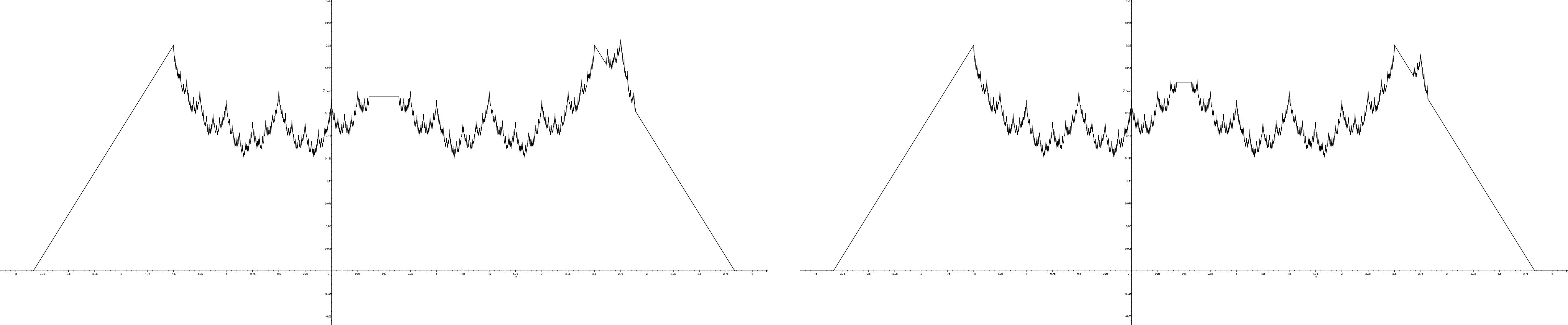
Figure 5: Functions $p_{1,n}$ and $p_{2,n}$ for $t=0.5$, $\beta=0.5$ and $n=50$

Following the lines of the proof of Proposition 3.3, both $p_{1,n}$ and $p_{2,n}$ are contained in the class $\mathscr{P}_{k}(L,\beta_{*},M,K_{R},\varepsilon)$ for sufficiently large $k\geq k_{0}(\beta_{*})$. Moreover, both $p_{1,n}$ and $p_{2,n}$ are constant on $B(t,c_{18}\cdot g_{\beta,n})$, so that

$$p_{1,n|B(t,c_{18}\cdot g_{\beta,n})},\,p_{2,n|B(t,c_{18}\cdot g_{\beta,n})}\in\mathcal{H}_{B(t,c_{18}\cdot g_{\beta,n})}(\infty,L)\$$

for some constant $L=L(\beta)$. Using Lemma 3.5 and (5.1), the absolute distance of the two hypotheses in $t$ is at least

$$|p_{1,n}(t)-p_{2,n}(t)| =|q_{t,n}(t;g_{\beta,n})-q_{t,n}(t;c_{18}\cdot g_{\beta,n})|$$

$$=\frac{1-2^{-\beta}}{12}|W_{\beta}(g_{\beta,n})-W_{\beta}(c_{18}\cdot g_{\beta,n})|$$

$$\geq\frac{1-2^{-\beta_{*}}}{12}\Big{(}|W_{\beta}(g_{\beta,n})-W_{\beta}(0)|-|W_{\beta}(c_{18}\cdot g_{\beta,n})-W_{\beta}(0)|\Big{)}$$

$$\geq\frac{1-2^{-\beta_{*}}}{12}\Big{(}g_{\beta,n}^{\beta}-L_{W}(\beta)\left(c_{18}\cdot g_{\beta,n}\right)^{\beta}\Big{)}$$

$$\geq 2c_{19}g_{\beta,n}^{\beta}$$

where

$$c_{19}=c_{19}(\beta_{*})=\frac{1-2^{-\beta_{*}}}{48}.$$

Since furthermore

$$\int(p_{2,n}(x)-p_{1,n}(x))\mathop{\mathrm{\mathstrut d}}\nolimits\!x=0,$$

and $\log(1+x)\leq x$ for $x>-1$, the Kullback-Leibler divergence between the associated product probability measures $\mathbb{P}_{1,n}^{\otimes n}$ and $\mathbb{P}_{2,n}^{\otimes n}$ is bounded from above by

$$K(\mathbb{P}_{2,n}^{\otimes n},\mathbb{P}_{1,n}^{\otimes n}) \leq n\,\int\frac{(p_{2,n}(x)-p_{1,n}(x))^{2}}{p_{1,n}(x)}\mathop{\mathrm{\mathstrut d}}\nolimits\!x$$

$$\leq 12\,n\,\int(p_{2,n}(x)-p_{1,n}(x))^{2}\mathop{\mathrm{\mathstrut d}}\nolimits\!x$$

$$=24\,n\,\int(q_{0,n}(x;g_{\beta,n})-q_{0,n}(x,c_{18}\cdot g_{\beta,n}))^{2}\mathop{\mathrm{\mathstrut d}}\nolimits\!x$$

$$=24\,n\,\left(\frac{1-2^{-\beta}}{12}\right)^{2}\Bigg{(}2\int_{c_{18}\cdot g_{\beta,n}}^{g_{\beta,n}}\Big{(}W_{\beta}(x)-W_{\beta}(g_{\beta,n})\Big{)}^{2}\mathop{\mathrm{\mathstrut d}}\nolimits\!x$$

$$\hskip 85.35826pt+\int_{-c_{18}\cdot g_{\beta,n}}^{c_{18}\cdot g_{\beta,n}}\Big{(}W_{\beta}(c_{18}\cdot g_{\beta,n})-W_{\beta}(g_{\beta,n})\Big{)}^{2}\mathop{\mathrm{\mathstrut d}}\nolimits\!x\Bigg{)}$$

$$\leq 24\,n\,L_{W}(\beta)^{2}\left(\frac{1-2^{-\beta}}{12}\right)^{2}\Bigg{(}2\int_{c_{18}\cdot g_{\beta,n}}^{g_{\beta,n}}(g_{\beta,n}-x)^{2\beta}\mathop{\mathrm{\mathstrut d}}\nolimits\!x$$

$$\hskip 199.16928pt+2(1-c_{18})^{2}c_{18}g_{\beta,n}^{2\beta+1}\Bigg{)}$$

$$=c_{20}$$

with

$$c_{20}=c_{20}(\beta)=48\,L_{W}(\beta)^{2}4^{-(2\beta+1)}\left(\frac{1-2^{-\beta}}{12}\right)^{2}\Bigg{(}\frac{(1-c_{18})^{2\beta+1}}{2\beta+1}+(1-c_{18})^{2}c_{18}\Bigg{)},$$

where we used Lemma 3.5 in the last inequality. Theorem 2.2 in Tsybakov (2009) then yields

$$\inf_{T_{n}}\sup_{p\in\mathscr{S}_{k}(\beta)}\mathbb{P}_{p}^{\otimes n}\left(n^{\frac{\beta}{2\beta+1}}\left|T_{n}(t)-p(t)\right|\geq c_{19}\right)$$

$$\hskip 142.26378pt\geq\max\left\{\frac{1}{4}\exp(-c_{20}),\,\frac{1-\sqrt{c_{20}/2}}{2}\right\}>0.$$

Part 2

For $\beta=1$, consider the function $p_{0}:\mathbb{R}\to\mathbb{R}$ with

$$p_{0}(x)=\begin{cases}0,\quad&\text{if }\ |x-t|>4\\ \frac{1}{4}-\frac{1}{16}|x-t|,\quad&\text{if }\ |x-t|\leq 4\end{cases}$$

and the functions $p_{1,n},p_{2,n}:\mathbb{R}\to\mathbb{R}$ with

$$p_{1,n}(x) =p_{0}(x)+q_{t+\frac{9}{4},n}(x;g_{1,n})-q_{t,n}(x;g_{1,n})$$

$$p_{2,n}(x) =p_{0}(x)+q_{t+\frac{9}{4},n}(x;g_{1,n}/2)-q_{t,n}(x;g_{1,n}/2)$$

for $g_{1,n}=\frac{1}{4}n^{-1/3}$, where

$$q_{a,n}(x;g)=\begin{cases}0,\quad&\text{if }\ |x-a|>g\\ \frac{1}{16}(g-|x-a|),\quad&\text{if }\ |x-a|\leq g\end{cases}$$

for $a\in\mathbb{R}$ and $g>0$. Following the lines of the proof of Proposition 3.3, both $p_{1,n}$ and $p_{2,n}$ are contained in the class $\mathscr{P}_{k}$ for sufficiently large $k\geq k_{0}(\beta_{*})$. Moreover, both $p_{1,n}$ and $p_{2,n}$ are constant on $B(t,g_{1,n}/2)$, so that

$$p_{1,n|B(t,g_{1,n}/2)},\,p_{2,n|B(t,g_{1,n}/2)}\in\mathcal{H}_{B(t,g_{1,n}/2)}(\infty,1/4).$$

The absolute distance of $p_{1,n}$ and $p_{2,n}$ in $t$ is given by

$$|p_{1,n}(t)-p_{2,n}(t)|=\frac{1}{32}g_{1,n},$$

whereas the Kullback-Leibler divergence between the associated product probability measures $\mathbb{P}_{1,n}^{\otimes n}$ and $\mathbb{P}_{2,n}^{\otimes n}$ is upper bounded by

$$K(\mathbb{P}_{2,n}^{\otimes n},\mathbb{P}_{1,n}^{\otimes n}) \leq n\,\int\frac{(p_{2,n}(x)-p_{1,n}(x))^{2}}{p_{1,n}(x)}\mathop{\mathrm{\mathstrut d}}\nolimits\!x$$

$$\leq 16\,n\,\int(p_{2,n}(x)-p_{1,n}(x))^{2}\mathop{\mathrm{\mathstrut d}}\nolimits\!x$$

$$=32\,n\,\int(q_{0,n}(x;g_{1,n})-q_{0,n}(x,g_{1,n}/2))^{2}\mathop{\mathrm{\mathstrut d}}\nolimits\!x$$

$$=32\,n\,\Bigg{(}2\int_{g_{1,n}/2}^{g_{1,n}}\left(\frac{1}{16}(g_{1,n}-x)\right)^{2}\mathop{\mathrm{\mathstrut d}}\nolimits\!x+\int_{-g_{1,n}/2}^{g_{1,n}/2}\Big{(}\frac{g_{1,n}}{32}\Big{)}^{2}\mathop{\mathrm{\mathstrut d}}\nolimits\!x\Bigg{)}$$

$$=\frac{2}{3\cdot 32^{2}}+\frac{1}{32}.$$

Together with Theorem 2.2 in Tsybakov (2009) the result follows.

Proof 5.10 (Proof of Theorem 3.12).

Recall the notation of Subsection 3.2, in particular the definitions of $\hat{h}_{n}^{loc}(t)$ in (3.12), of $q_{n}(\alpha)$ in (3.14), of $\beta_{n,p}(t)$ in (3.15), and of $\bar{h}_{n}(t)$ in (4.1). Furthermore, set $\tilde{\gamma}=\tilde{\gamma}(c_{1})=\frac{1}{2}(c_{1}\log 2-1)$. To show that the confidence band is adaptive, note that according to Proposition 4.1 and Lemma 4.2 for any $\delta>0$ there exists some $n_{0}(\delta)$, such that

$$\sup_{p\in\mathscr{P}_{n}}\mathbb{P}_{p}^{\chi_{2}}\left(\sup_{t\in[0,1]}|C_{n,\alpha}(t)|\cdot\left(\frac{\log\tilde{n}}{\tilde{n}}\right)^{\frac{-\beta_{n,p}(t)}{2\beta_{n,p}(t)+1}}\geq\sqrt{6}\cdot 2^{1-\frac{j_{\min}}{2}}q_{n}(\alpha)(\log\tilde{n})^{\tilde{\gamma}}\right)$$

$$\quad=\sup_{p\in\mathscr{P}_{n}}\mathbb{P}_{p}^{\chi_{2}}\left(\sup_{t\in[0,1]}\frac{\bar{h}_{n}(t)}{\hat{h}_{n}^{loc}(t)}\cdot 2^{-u_{n}}\geq 6\right)$$

$$\quad=\sup_{p\in\mathscr{P}_{n}}\mathbb{P}_{p}^{\chi_{2}}\left(\max_{k\in T_{n}}\,\sup_{t\in I_{k}}\,\frac{\bar{h}_{n}(t)}{\min\left\{2^{-\hat{j}_{n}((k-1)\delta_{n})},2^{-\hat{j}_{n}(k\delta_{n})}\right\}}\geq 6\right)$$

$$\quad\leq\sup_{p\in\mathscr{P}_{n}}\mathbb{P}_{p}^{\chi_{2}}\left(\max_{k\in T_{n}}\,\frac{\min\left\{\bar{h}_{n}((k-1)\delta_{n}),\bar{h}_{n}(k\delta_{n})\right\}}{\min\left\{2^{-\hat{j}_{n}((k-1)\delta_{n})},2^{-\hat{j}_{n}(k\delta_{n})}\right\}}\geq 2\right)$$

$$\quad\leq\sup_{p\in\mathscr{P}_{n}}\mathbb{P}_{p}^{\chi_{2}}\left(\exists\,k\in T_{n}:\frac{\min\left\{2^{-\bar{j}_{n}((k-1)\delta_{n})},2^{-\bar{j}_{n}(k\delta_{n})}\right\}}{\min\left\{2^{-\hat{j}_{n}((k-1)\delta_{n})},2^{-\hat{j}_{n}(k\delta_{n})}\right\}}\geq 1\right)$$

$$\quad=\sup_{p\in\mathscr{P}_{n}}\left\{1-\mathbb{P}_{p}^{\chi_{2}}\left(\forall\,k\in T_{n}:\frac{\min\left\{2^{-\bar{j}_{n}((k-1)\delta_{n})},2^{-\bar{j}_{n}(k\delta_{n})}\right\}}{\min\left\{2^{-\hat{j}_{n}((k-1)\delta_{n})},2^{-\hat{j}_{n}(k\delta_{n})}\right\}}<1\right)\right\}$$

$$\quad\leq\sup_{p\in\mathscr{P}_{n}}\left\{1-\mathbb{P}_{p}^{\chi_{2}}\left(\hat{j}_{n}(k\delta_{n})<\bar{j}_{n}(k\delta_{n})\text{ for all }k\in T_{n}\right)\right\}$$

$$\quad\leq\delta$$

for all $n\geq n_{0}(\delta)$.

5.2 Proofs of the results in Section 4

Proof 5.11 (Proof of Proposition 4.1).

We prove first that

$$\lim_{n\to\infty}\sup_{p\in\mathscr{P}_{n}}\mathbb{P}_{p}^{\chi_{2}}\left(\hat{j}_{n}(k\delta_{n})>\bar{j}_{n}(k\delta_{n})+1\text{ for some }k\in T_{n}\right)=0.$$ (5.25)

Note first that if $\hat{j}_{n}(k\delta_{n})>\bar{j}_{n}(k\delta_{n})+1$ for some $k\in T_{n}$, then $\bar{j}_{n}(k\delta_{n})+1$ cannot be an admissible exponent according to the construction of the bandwidth selection scheme in (3.10), that is, $\bar{j}_{n}(k\delta_{n})+1\notin\mathcal{A}_{n}(k\delta_{n})$. By definition of $\mathcal{A}_{n}(k\delta_{n})$ there exist exponents $m_{n,k},m_{n,k}^{\prime}\in\mathcal{J}_{n}$ with $m_{n,k}>m_{n,k}^{\prime}\geq\bar{j}_{n}(k\delta_{n})+4$ such that

$$\max_{s\in B\left(k\delta_{n},\frac{7}{8}\cdot 2^{-(\bar{j}_{n}(k\delta_{n})+1)}\right)\cap\mathcal{H}_{n}}|\hat{p}_{n}^{(2)}(s,m_{n,k})-\hat{p}_{n}^{(2)}(s,m_{n,k}^{\prime})|>c_{2}\sqrt{\frac{\log\tilde{n}}{\tilde{n}2^{-m_{n,k}}}}.$$

Consequently,

$$\mathbb{P}_{p}^{\chi_{2}}\left(\hat{j}_{n}(k\delta_{n})>\bar{j}_{n}(k\delta_{n})+1\text{ for some }k\in T_{n}\right)$$

$$\leq\mathbb{P}_{p}^{\chi_{2}}\Bigg{(}\exists k\in T_{n}\text{ and }\exists\,m_{n,k},m_{n,k}^{\prime}\in\mathcal{J}_{n}\text{ with }m_{n,k}>m_{n,k}^{\prime}\geq\bar{j}_{n}(k\delta_{n})+4\text{ such that }$$

$$\max_{s\in B\left(k\delta_{n},\frac{7}{8}\cdot 2^{-(\bar{j}_{n}(k\delta_{n})+1)}\right)\cap\mathcal{H}_{n}}|\hat{p}_{n}^{(2)}(s,m_{n,k})-\hat{p}_{n}^{(2)}(s,m_{n,k}^{\prime})|>c_{2}\sqrt{\frac{\log\tilde{n}}{\tilde{n}2^{-m_{n,k}}}}\,\Bigg{)}$$

$$\leq\sum_{m\in\mathcal{J}_{n}}\sum_{m^{\prime}\in\mathcal{J}_{n}}\mathbb{P}_{p}^{\chi_{2}}\Bigg{(}m>m^{\prime}\geq\bar{j}_{n}(k\delta_{n})+4\text{ and }$$

$$\hskip 76.82234pt\max_{s\in B\left(k\delta_{n},\frac{7}{8}\cdot 2^{-(\bar{j}_{n}(k\delta_{n})+1)}\right)\cap\mathcal{H}_{n}}|\hat{p}_{n}^{(2)}(s,m)-\hat{p}_{n}^{(2)}(s,m^{\prime})|$$

$$\hskip 199.16928pt>c_{2}\sqrt{\frac{\log\tilde{n}}{\tilde{n}2^{-m}}}\text{ for some }k\in T_{n}\Bigg{)}.$$

We furthermore use the following decomposition into two stochastic terms and two bias terms

$$\max_{s\in B\left(k\delta_{n},\frac{7}{8}\cdot 2^{-(\bar{j}_{n}(k\delta_{n})+1)}\right)\cap\mathcal{H}_{n}}\left|\hat{p}_{n}^{(2)}(s,m)-\hat{p}_{n}^{(2)}(s,m^{\prime})\right|$$

$$\quad\leq\max_{s\in B\left(k\delta_{n},\frac{7}{8}\cdot 2^{-(\bar{j}_{n}(k\delta_{n})+1)}\right)\cap\mathcal{H}_{n}}\left|\hat{p}_{n}^{(2)}(s,m)-\mathbb{E}_{p}^{\chi_{2}}\hat{p}_{n}^{(2)}(s,m)\right|$$

$$\hskip 56.9055pt+\max_{s\in B\left(k\delta_{n},\frac{7}{8}\cdot 2^{-(\bar{j}_{n}(k\delta_{n})+1)}\right)\cap\mathcal{H}_{n}}\left|\hat{p}_{n}^{(2)}(s,m^{\prime})-\mathbb{E}_{p}^{\chi_{2}}\hat{p}_{n}^{(2)}(s,m^{\prime})\right|$$

$$\qquad+\sup_{s\in B\left(k\delta_{n},\frac{7}{8}\cdot 2^{-(\bar{j}_{n}(k\delta_{n})+1)}\right)}\left|\mathbb{E}_{p}^{\chi_{2}}\hat{p}_{n}^{(2)}(s,m)-p(s)\right|$$

$$\qquad+\sup_{s\in B\left(k\delta_{n},\frac{7}{8}\cdot 2^{-(\bar{j}_{n}(k\delta_{n})+1)}\right)}\left|\mathbb{E}_{p}^{\chi_{2}}\hat{p}_{n}^{(2)}(s,m^{\prime})-p(s)\right|.$$

In order to bound the two bias terms, note first that for any $m>m^{\prime}\geq\bar{j}_{n}(k\delta_{n})+4$ both

$$\frac{7}{8}\cdot 2^{-(\bar{j}_{n}(k\delta_{n})+1)}=2^{-(\bar{j}_{n}(k\delta_{n})+1)}-\frac{1}{8}\cdot 2^{-(\bar{j}_{n}(k\delta_{n})+1)}\leq 2^{-(\bar{j}_{n}(k\delta_{n})+1)}-2^{-m}$$

and

$$\frac{7}{8}\cdot 2^{-(\bar{j}_{n}(k\delta_{n})+1)}=2^{-(\bar{j}_{n}(k\delta_{n})+1)}-\frac{1}{8}\cdot 2^{-(\bar{j}_{n}(k\delta_{n})+1)}\leq 2^{-(\bar{j}_{n}(k\delta_{n})+1)}-2^{-m^{\prime}}.$$

According to Assumption 3.1 and Lemma 3.2,

$$p_{|B\left(k\delta_{n},2^{-(\bar{j}_{n}(k\delta_{n})+1)}\right)}\in\mathcal{H}_{\beta^{*},B\left(k\delta_{n},2^{-(\bar{j}_{n}(k\delta_{n})+1)}\right)}\left(\beta_{p}\left(B\left(k\delta_{n},2^{-\bar{j}_{n}(k\delta_{n})}\right)\right),L^{*}\right),$$

so that Lemma 4.4 yields,

$$\sup_{s\in B\left(k\delta_{n},\frac{7}{8}\cdot 2^{-(\bar{j}_{n}(k\delta_{n})+1)}\right)}\left|\mathbb{E}_{p}^{\chi_{2}}\hat{p}_{n}^{(2)}(s,m)-p(s)\right|$$

$$\hskip 113.81102pt\leq\sup_{s\in B(k\delta_{n},2^{-(\bar{j}_{n}(k\delta_{n})+1)}-2^{-m})}\left|\mathbb{E}_{p}^{\chi_{2}}\hat{p}_{n}^{(2)}(s,m)-p(s)\right|$$

$$\hskip 113.81102pt\leq b_{2}2^{-m\beta_{p}\left(B\left(k\delta_{n},2^{-\bar{j}_{n}(k\delta_{n})}\right)\right)}$$

$$\hskip 113.81102pt\leq b_{2}2^{-m\beta_{p}\left(B\left(k\delta_{n},\bar{h}_{n}(k\delta_{n})\right)\right)}$$

$$\hskip 113.81102pt\leq b_{2}2^{-m\beta_{n,p}(k\delta_{n})},$$

with the bandwidth $\bar{h}_{n}(\cdot)$ as defined in (4.1), and analogously

$$\sup_{s\in B\left(k\delta_{n},\frac{7}{8}\cdot 2^{-(\bar{j}_{n}(k\delta_{n})+1)}\right)}\left|\mathbb{E}_{p}^{\chi_{2}}\hat{p}_{n}^{(2)}(s,m^{\prime})-p(s)\right|\leq b_{2}2^{-m^{\prime}\beta_{n,p}(k\delta_{n})}.$$

Thus, the sum of the two bias terms is bounded from above by $2b_{2}\bar{h}_{n}(k\delta_{n})^{\beta_{n,p}(k\delta_{n})}$, such that

$$\sqrt{\frac{\tilde{n}2^{-m}}{\log\tilde{n}}}\Bigg{(}\sup_{s\in B\left(k\delta_{n},\frac{7}{8}\cdot 2^{-(\bar{j}_{n}(k\delta_{n})+1)})\right)}\left|\mathbb{E}_{p}^{\chi_{2}}\hat{p}_{n}^{(2)}(s,m)-p(s)\right|$$

$$\hskip 85.35826pt+\sup_{s\in B\left(k\delta_{n},\frac{7}{8}\cdot 2^{-(\bar{j}_{n}(k\delta_{n})+1)})\right)}\left|\mathbb{E}_{p}^{\chi_{2}}\hat{p}_{n}^{(2)}(s,m^{\prime})-p(s)\right|\Bigg{)}$$

$$\quad\leq\sqrt{\frac{\tilde{n}\bar{h}_{n}(k\delta_{n})}{\log\tilde{n}}}\cdot 2b_{2}\bar{h}_{n}(k\delta_{n})^{\beta_{n,p}(k\delta_{n})}$$

$$\quad\leq c_{21},$$

where $c_{21}=c_{21}(\beta_{*},L^{*},\varepsilon)=2b_{2}\cdot 2^{-j_{\min}(2\beta_{*}+1)/2}$. Thus, it holds

$$\mathbb{P}_{p}^{\chi_{2}}\left(\hat{j}_{n}(k\delta_{n})>\bar{j}_{n}(k\delta_{n})+1\text{ for some }k\in T_{n}\right)$$

$$\quad\leq\sum_{m\in\mathcal{J}_{n}}\sum_{m^{\prime}\in\mathcal{J}_{n}}\Bigg{\{}\mathbb{P}_{p}^{\chi_{2}}\Bigg{(}\max_{k\in T_{n}}\max_{s\in B\left(k\delta_{n},\frac{7}{8}\cdot 2^{-(\bar{j}_{n}(k\delta_{n})+1)}\right)\cap\mathcal{H}_{n}}\left|\hat{p}_{n}^{(2)}(s,m)-\mathbb{E}_{p}^{\chi_{2}}\hat{p}_{n}^{(2)}(s,m)\right|$$

$$\hskip 270.30118pt>\frac{c_{2}-c_{21}}{2}\sqrt{\frac{\log\tilde{n}}{\tilde{n}2^{-m}}}\,\Bigg{)}$$

$$\hskip 54.06006pt+\mathbb{P}_{p}^{\chi_{2}}\Bigg{(}\max_{k\in T_{n}}\max_{s\in B\left(k\delta_{n},\frac{7}{8}\cdot 2^{-(\bar{j}_{n}(k\delta_{n})+1)}\right)\cap\mathcal{H}_{n}}\left|\hat{p}_{n}^{(2)}(s,m^{\prime})-\mathbb{E}_{p}^{\chi_{2}}\hat{p}_{n}^{(2)}(s,m^{\prime})\right|$$

$$\hskip 247.53888pt>\frac{c_{2}-c_{21}}{2}\sqrt{\frac{\log\tilde{n}}{\tilde{n}2^{-m^{\prime}}}}\,\Bigg{)}\Bigg{\}}$$

$$\quad\leq 2\,|\mathcal{J}_{n}|^{2}\cdot\mathbb{P}_{p}^{\chi_{2}}\left(\sup_{s\in\mathcal{H}_{n}}\max_{h\in\mathcal{G}_{n}}\sqrt{\frac{\tilde{n}h}{\log\tilde{n}}}\left|\hat{p}_{n}^{(2)}(s,h)-\mathbb{E}_{p}^{\chi_{2}}\hat{p}_{n}^{(2)}(s,h)\right|>\frac{c_{2}-c_{21}}{2}\right).$$

Choose $c_{2}=c_{2}(A,\nu,\beta_{*},L^{*},K,\varepsilon)$ sufficiently large such that $c_{2}\geq c_{21}+2\eta_{0}$, where $\eta_{0}$ is given in Lemma 4.3. Then, Lemma 4.3 and the logarithmic cardinality of $\mathcal{J}_{n}$ yield (5.25). In addition, we show that

$$\lim_{n\to\infty}\sup_{p\in\mathscr{P}_{n}}\mathbb{P}_{p}^{\chi_{2}}\left(\hat{j}_{n}(k\delta_{n})<k_{n}(k\delta_{n})\text{ for some }k\in T_{n}\right)=0.$$ (5.26)

For $t\in[0,1]$, due to the sequential definition of the set of admissible bandwidths $\mathcal{A}_{n}(t)$ in (3.10), if $\hat{j}_{n}(t)<j_{\max}$, then both $\hat{j}_{n}(t)$ and $\hat{j}_{n}(t)+1$ are contained in $\mathcal{A}_{n}(t)$. Note furthermore, that $k_{n}(t)<j_{\max}$ for any $t\in[0,1]$. Thus, if $\hat{j}_{n}(k\delta_{n})<k_{n}(k\delta_{n})$ for some $k\in T_{n}$, there exists some index $j<k_{n}(k\delta_{n})+1$ with $j\in\mathcal{A}_{n}(k\delta_{n})$ and satisfying (3.6) and (3.7) for $u=2^{-j}$ and $t=k\delta_{n}$. In particular,

$$\max_{s\in B\left(k\delta_{n},\frac{7}{8}\cdot 2^{-j}\right)\cap\mathcal{H}_{n}}\left|\hat{p}_{n}^{(2)}(s,j+3)-\hat{p}_{n}^{(2)}(s,\bar{j}_{n}(k\delta_{n}))\right|\leq c_{2}\sqrt{\frac{\log\tilde{n}}{\tilde{n}2^{-\bar{j}_{n}(k\delta_{n})}}}$$

for sufficiently large $n\geq n_{0}(c_{1})$, using that $\bar{j}_{n}(k\delta_{n})\in\mathcal{J}_{n}$ for any $k\in T_{n}$. Consequently

$$\mathbb{P}_{p}^{\chi_{2}}\left(\hat{j}_{n}(k\delta_{n})<k_{n}(k\delta_{n})\text{ for some }k\in T_{n}\right)$$

$$\begin{split}&\leq\sum_{j\in\mathcal{J}_{n}}\mathbb{P}_{p}^{\chi_{2}}\Bigg{(}\exists\,k\in T_{n}:j<k_{n}(k\delta_{n})+1\text{ and }p_{|B(k\delta_{n},2^{-j})}\in\mathcal{H}_{\beta^{*},B(k\delta_{n},2^{-j})}(\beta,L^{*})\\ &\hskip 56.9055pt\text{and}\sup_{s\in B(k\delta_{n},2^{-j}-g)}\left|(K_{g}\ast p)(s)-p(s)\right|\geq\frac{g^{\beta}}{\log n}\text{ for all }g\in\mathcal{G}_{\infty}\text{ with }\\ &\hskip 56.9055ptg\leq 2^{-(j+3)}\text{ and }\max_{s\in B\left(k\delta_{n},\frac{7}{8}\cdot 2^{-j}\right)\cap\mathcal{H}_{n}}\left|\hat{p}_{n}^{(2)}(s,j+3)-\hat{p}_{n}^{(2)}(s,\bar{j}_{n}(k\delta_{n}))\right|\\ &\hskip 270.30118pt\leq c_{2}\sqrt{\frac{\log\tilde{n}}{\tilde{n}2^{-\bar{j}_{n}(k\delta_{n})}}}\,\Bigg{)}.\end{split}$$ (5.27)

The triangle inequality yields

$$\max_{s\in B\left(k\delta_{n},\frac{7}{8}\cdot 2^{-j}\right)\cap\mathcal{H}_{n}}\left|\hat{p}_{n}^{(2)}(s,j+3)-\hat{p}_{n}^{(2)}(s,\bar{j}_{n}(k\delta_{n}))\right|$$

$$\hskip 56.9055pt\geq\max_{s\in B\left(k\delta_{n},\frac{7}{8}\cdot 2^{-j}\right)\cap\mathcal{H}_{n}}\left|\mathbb{E}_{p}^{\chi_{2}}\hat{p}_{n}^{(2)}(s,j+3)-\mathbb{E}_{p}^{\chi_{2}}\hat{p}_{n}^{(2)}(s,\bar{j}_{n}(k\delta_{n}))\right|$$

$$\hskip 85.35826pt-\max_{s\in B\left(k\delta_{n},\frac{7}{8}\cdot 2^{-j}\right)\cap\mathcal{H}_{n}}\left|\hat{p}_{n}^{(2)}(s,j+3)-\mathbb{E}_{p}^{\chi_{2}}\hat{p}_{n}^{(2)}(s,j+3)\right|$$

$$\hskip 85.35826pt-\max_{s\in B\left(k\delta_{n},\frac{7}{8}\cdot 2^{-j}\right)\cap\mathcal{H}_{n}}\left|\hat{p}_{n}^{(2)}(s,\bar{j}_{n}(k\delta_{n}))-\mathbb{E}_{p}^{\chi_{2}}\hat{p}_{n}^{(2)}(s,\bar{j}_{n}(k\delta_{n}))\right|.$$

We further decompose

$$\max_{s\in B\left(k\delta_{n},\frac{7}{8}\cdot 2^{-j}\right)\cap\mathcal{H}_{n}}\left|\mathbb{E}_{p}^{\chi_{2}}\hat{p}_{n}^{(2)}(s,j+3)-\mathbb{E}_{p}^{\chi_{2}}\hat{p}_{n}^{(2)}(s,\bar{j}_{n}(k\delta_{n}))\right|$$

$$\hskip 113.81102pt\geq\max_{s\in B\left(k\delta_{n},\frac{7}{8}\cdot 2^{-j}\right)\cap\mathcal{H}_{n}}\left|\mathbb{E}_{p}^{\chi_{2}}\hat{p}_{n}^{(2)}(s,j+3)-p(s)\right|$$

$$\hskip 142.26378pt\quad-\sup_{s\in B\left(k\delta_{n},\frac{7}{8}\cdot 2^{-j}\right)}\left|\mathbb{E}_{p}^{\chi_{2}}\hat{p}_{n}^{(2)}(s,\bar{j}_{n}(k\delta_{n}))-p(s)\right|.$$

As Assumption 3.1 is satisfied for $u=2^{-j}$ and $t=k\delta_{n}$, together with Lemma 3.2 we both have

$$p_{|B\left(k\delta_{n},2^{-j}\right)}\in\mathcal{H}_{\beta^{*},B\left(k\delta_{n},2^{-j}\right)}\Big{(}\beta_{p}\left(B\left(k\delta_{n},2^{-j}\right)\right),L^{*}\Big{)}$$ (5.28)

and

$$\sup_{s\in B\left(k\delta_{n},2^{-j}-g\right)}\left|(K_{g}\ast p)(s)-p(s)\right|\geq\frac{g^{\beta_{p}\left(B\left(k\delta_{n},2^{-j}\right)\right)}}{\log n}$$ (5.29)

for all $g\in\mathcal{G}_{\infty}$ with $g\leq 2^{-(j+3)}$. In particular, (5.28) together with Lemma 4.4 gives the upper bias bound

$$\sup_{s\in B\left(k\delta_{n},\frac{7}{8}\cdot 2^{-j}\right)}\Big{|}\mathbb{E}_{p}^{\chi_{2}}\hat{p}_{n}^{(2)}(s,\bar{j}_{n}(k\delta_{n}))-p(s)\Big{|}\leq b_{2}\cdot 2^{-\bar{j}_{n}(k\delta_{n})\beta_{p}\left(B\left(k\delta_{n},2^{-j}\right)\right)}$$

for sufficiently large $n\geq n_{0}(c_{1})$, whereas (5.29) yields the bias lower bound

$$\sup_{s\in B\left(k\delta_{n},\frac{7}{8}\cdot 2^{-j}\right)}\left|\mathbb{E}_{p}^{\chi_{2}}\hat{p}_{n}^{(2)}(s,j+3)-p(s)\right|$$

$$\hskip 56.9055pt=\sup_{s\in B(k\delta_{n},2^{-j}-2^{-(j+3)})}\left|\mathbb{E}_{p}^{\chi_{2}}\hat{p}_{n}^{(2)}(s,j+3)-p(s)\right|$$

$$\hskip 56.9055pt\geq\frac{2^{-(j+3)\beta_{p}\left(B\left(k\delta_{n},2^{-j}\right)\right)}}{\log n}.$$ (5.30)

To show that the above lower bound even holds for the maximum over the set $B\left(k\delta_{n},\frac{7}{8}\cdot 2^{-j}\right)\cap\mathcal{H}_{n}$, note that for any point $k\delta_{n}-\frac{7}{8}2^{-j}\leq\tilde{t}\leq k\delta_{n}+\frac{7}{8}2^{-j}$ there exists some $t\in\mathcal{H}_{n}$ with $|t-\tilde{t}|\leq\delta_{n}$, and

$$\left|\mathbb{E}_{p}^{\chi_{2}}\hat{p}_{n}^{(2)}(t,j+3)-p(t)\right|$$

$$\hskip 56.9055pt=\left|\int K(x)\Big{\{}p(t+2^{-(j+3)}x)-p(t)\Big{\}}\mathop{\mathrm{\mathstrut d}}\nolimits\!x\right|$$

$$\hskip 56.9055pt\geq\left|\int K(x)\Big{\{}p\left(\tilde{t}+2^{-(j+3)}x\right)-p\left(\tilde{t}\,\right)\Big{\}}\mathop{\mathrm{\mathstrut d}}\nolimits\!x\right|$$

$$\hskip 56.9055pt\qquad-\int|K(x)|\cdot\left|p(t+2^{-(j+3)}x)-p\left(\tilde{t}+2^{-(j+3)}x\right)\right|\mathop{\mathrm{\mathstrut d}}\nolimits\!x$$

$$\hskip 56.9055pt\qquad-\int|K(x)|\cdot|p(t)-p\left(\tilde{t}\right)|\mathop{\mathrm{\mathstrut d}}\nolimits\!x$$

$$\hskip 56.9055pt\geq\left|\int K(x)\Big{\{}p\left(\tilde{t}+2^{-(j+3)}x\right)-p\left(\tilde{t}\right)\Big{\}}\mathop{\mathrm{\mathstrut d}}\nolimits\!x\right|-2\|K\|_{1}L^{*}\cdot|t-\tilde{t}|^{\beta_{*}},$$ (5.31)

where

$$|t-\tilde{t}|^{\beta_{*}} \leq\delta_{n}^{\beta_{*}}$$

$$\leq 2^{-j_{\min}}\left(\frac{\log\tilde{n}}{\tilde{n}}\right)^{\frac{1}{2}}(\log\tilde{n})^{-2}$$

$$\leq\frac{\bar{h}_{n}(k\delta_{n})^{\beta_{n,p}(k\delta_{n})}}{(\log\tilde{n})^{2}}$$

$$\leq\frac{2^{-(\bar{j}_{n}(k\delta_{n})-1)\beta_{n,p}(k\delta_{n})}}{(\log\tilde{n})^{2}}$$

$$\leq\frac{2^{-(j+3)\beta_{n,p}(k\delta_{n})}}{(\log\tilde{n})^{2}}$$

for sufficiently large $n\geq n_{0}(c_{1})$. For $n\geq n_{0}(c_{1})$ and $j\in\mathcal{J}_{n}$ with $j<k_{n}(k\delta_{n})+1$,

$$2^{-j}>2^{m_{n}-1}\cdot 2^{-\bar{j}_{n}(k\delta_{n})}>\bar{h}_{n}(k\delta_{n}).$$

Together with (5.28), this implies

$$\beta_{p}(B(k\delta_{n},2^{-j}))\leq\beta_{n,p}(k\delta_{n})$$ (5.32)

since otherwise $p$ would be $\beta$-Hölder smooth with $\beta>\beta_{n,p}(k\delta_{n})$ on a ball $B(k\delta_{n},r)$ with radius $r>\bar{h}_{n}(t)$, which would contradict the definition of $\beta_{n,p}(k\delta_{n})$ together with Lemma A.7. This implies

$$|t-\tilde{t}|^{\beta_{*}}\leq\frac{2^{-(j+3)\beta_{p}(B(k\delta_{n},2^{-j}))}}{(\log\tilde{n})^{2}}.$$

Together with inequalities (5.11) and (5.11),

$$\max_{s\in B\left(k\delta_{n},\frac{7}{8}\cdot 2^{-j}\right)\cap\mathcal{H}_{n}}\left|\mathbb{E}_{p}^{\chi_{2}}\hat{p}_{n}^{(2)}(s,j+3)-p(s)\right|$$

$$\qquad\qquad\quad\geq\sup_{s\in B\left(k\delta_{n},\frac{7}{8}\cdot 2^{-j}\right)}\left|\mathbb{E}_{p}^{\chi_{2}}\hat{p}_{n}^{(2)}(s,j+3)-p(s)\right|-2\|K\|_{1}L^{*}\frac{2^{-(j+3)\beta_{p}(B(k\delta_{n},2^{-j}))}}{(\log\tilde{n})^{2}}$$

$$\qquad\qquad\quad\geq\frac{1}{2}\cdot\frac{2^{-(j+3)\beta_{p}(B(k\delta_{n},2^{-j}))}}{\log\tilde{n}}$$

for sufficiently large $n\geq n_{0}(L^{*},K,c_{1})$. Altogether, we get for $j<k_{n}(k\delta_{n})+1$,

$$\sqrt{\frac{\tilde{n}2^{-\bar{j}_{n}(k\delta_{n})}}{\log\tilde{n}}}\max_{s\in B\left(k\delta_{n},\frac{7}{8}\cdot 2^{-j}\right)\cap\mathcal{H}_{n}}\left|\mathbb{E}_{p}^{\chi_{2}}\hat{p}_{n}^{(2)}(s,j+3)-\mathbb{E}_{p}^{\chi_{2}}\hat{p}_{n}^{(2)}(s,\bar{j}_{n}(k\delta_{n}))\right|$$

$$\geq\sqrt{\frac{\tilde{n}2^{-\bar{j}_{n}(k\delta_{n})}}{\log\tilde{n}}}\Bigg{(}\max_{s\in B\left(k\delta_{n},\frac{7}{8}\cdot 2^{-j}\right)\cap\mathcal{H}_{n}}\left|\mathbb{E}_{p}^{\chi_{2}}\hat{p}_{n}^{(2)}(s,j+3)-p(s)\right|$$

$$\hskip 113.81102pt-\max_{s\in B\left(k\delta_{n},\frac{7}{8}\cdot 2^{-j}\right)\cap\mathcal{H}_{n}}\left|\mathbb{E}_{p}^{\chi_{2}}\hat{p}_{n}^{(2)}(s,\bar{j}_{n}(k\delta_{n}))-p(s)\right|\Bigg{)}$$

$$\geq\sqrt{\frac{\tilde{n}\bar{h}_{n}(k\delta_{n})}{2\log\tilde{n}}}\left(\frac{1}{2}\cdot\frac{2^{-(j+3)\beta_{p}(B(k\delta_{n},2^{-j}))}}{\log\tilde{n}}-b_{2}\cdot 2^{-\bar{j}_{n}(k\delta_{n})\beta_{p}\left(B\left(k\delta_{n},2^{-j}\right)\right)}\right)$$

$$\geq\sqrt{\frac{\tilde{n}\bar{h}_{n}(k\delta_{n})}{2\log\tilde{n}}}2^{-(\bar{j}_{n}(k\delta_{n})-1)\beta_{p}(B(k\delta_{n},2^{-j}))}\left(\frac{1}{2}\cdot\frac{2^{(\bar{j}_{n}(k\delta_{n})-j-4)\beta_{p}(B(k\delta_{n},2^{-j}))}}{\log\tilde{n}}-b_{2}2^{-\beta_{*}}\right)$$

$$>\sqrt{\frac{\tilde{n}\bar{h}_{n}(k\delta_{n})}{2\log\tilde{n}}}2^{-(\bar{j}_{n}(k\delta_{n})-1)\beta_{p}(B(k\delta_{n},2^{-j}))}\left(\frac{2^{(m_{n}-5)\beta_{*}}}{2\,\log\tilde{n}}-b_{2}2^{-\beta_{*}}\right).$$

We now show that for $j\in\mathcal{J}_{n}$ with $j<k_{n}(k\delta_{n})+1$, we have that

$$\beta_{p}(B(k\delta_{n},2^{-j}))\leq\beta^{*}.$$ (5.33)

According to (5.32), it remains to show that $\beta_{n,p}(k\delta_{n})\leq\beta^{*}$. If $\beta_{n,p}(k\delta_{n})=\infty$, then $\bar{j}_{n}(k\delta_{n})=j_{\min}$. Since furthermore $j\in\mathcal{J}_{n}$ and therefore $j\geq j_{\min}$, this immediately contradicts $j<k_{n}(k\delta_{n})+1$. That is, $j<k_{n}(k\delta_{n})+1$ implies that $\beta_{n,p}(k\delta_{n})<\infty$, which in turn implies $\beta_{n,p}(k\delta_{n})\leq\beta^{*}$ according to Remark 3. Due to (3.9) and (5.33), the last expression is again lower bounded by

$$3c_{2}\sqrt{\frac{\tilde{n}\bar{h}_{n}(k\delta_{n})}{\log\tilde{n}}}\bar{h}_{n}(k\delta_{n})^{\beta_{p}(B(k\delta_{n},2^{-j}))}2^{j_{\min}\frac{2\beta_{p}(B(k\delta_{n},2^{-j}))+1}{2}}$$

for sufficiently large $n\geq n_{0}(L^{*},K,\beta_{*},\beta^{*},c_{1},c_{2})$. Recalling (5.32), we obtain

$$\sqrt{\frac{\tilde{n}2^{-\bar{j}_{n}(k\delta_{n})}}{\log\tilde{n}}}\max_{s\in B\left(k\delta_{n},\frac{7}{8}\cdot 2^{-j}\right)\cap\mathcal{H}_{n}}\left|\mathbb{E}_{p}^{\chi_{2}}\hat{p}_{n}^{(2)}(s,j+3)-\mathbb{E}_{p}^{\chi_{2}}\hat{p}_{n}^{(2)}(s,\bar{j}_{n}(k\delta_{n}))\right|$$

$$\qquad\geq 3c_{2}\sqrt{\frac{\tilde{n}\bar{h}_{n}(k\delta_{n})}{\log\tilde{n}}}\bar{h}_{n}(k\delta_{n})^{\beta_{n,p}(k\delta_{n})}2^{j_{\min}\frac{2\beta_{p}(B(k\delta_{n},2^{-j}))+1}{2}}$$

$$\qquad=3c_{2}.$$

Thus, by the above consideration and (5.11),

$$\mathbb{P}_{p}^{\chi_{2}}\left(\hat{j}_{n}(k\delta_{n})<k_{n}(k\delta_{n})\text{ for some }k\in T_{n}\right)\leq\sum_{j\in\mathcal{J}_{n}}\left(P_{j,1}+P_{j,2}\right)$$

for sufficiently large $n\geq n_{0}(L^{*},K,\beta_{*},\beta^{*},c_{1},c_{2})$, with

$$P_{j,1} =\mathbb{P}_{p}^{\chi_{2}}\Bigg{(}\exists k\in T_{n}:j<k_{n}(k\delta_{n})+1\text{ and }\sqrt{\frac{\tilde{n}2^{-(j+3)}}{\log\tilde{n}}}$$

$$\hskip 42.67912pt\cdot\max_{s\in B\left(k\delta_{n},\frac{7}{8}\cdot 2^{-j}\right)\cap\mathcal{H}_{n}}\left|\hat{p}_{n}^{(2)}(s,j+3)-\mathbb{E}_{p}^{\chi_{2}}\hat{p}_{n}^{(2)}(s,j+3)\right|\geq c_{2}\Bigg{)}$$

$$P_{j,2} =\mathbb{P}_{p}^{\chi_{2}}\Bigg{(}\exists k\in T_{n}:j<k_{n}(k\delta_{n})+1\text{ and }\sqrt{\frac{\tilde{n}2^{-\bar{j}_{n}(k\delta_{n})}}{\log\tilde{n}}}$$

$$\hskip 5.69046pt\cdot\max_{s\in B\left(k\delta_{n},\frac{7}{8}\cdot 2^{-j}\right)\cap\mathcal{H}_{n}}\left|\hat{p}_{n}^{(2)}(s,\bar{j}_{n}(k\delta_{n}))-\mathbb{E}_{p}^{\chi_{2}}\hat{p}_{n}^{(2)}(s,\bar{j}_{n}(k\delta_{n}))\right|\geq c_{2}\Bigg{)}.$$

Both $P_{j,1}$ and $P_{j,2}$ are bounded by

$$P_{j,i}\leq\mathbb{P}_{p}^{\chi_{2}}\left(\sup_{s\in\mathcal{H}_{n}}\max_{h\in\mathcal{G}_{n}}\sqrt{\frac{\tilde{n}h}{\log\tilde{n}}}\left|\hat{p}_{n}^{(2)}(s,h)-\mathbb{E}_{p}^{\chi_{2}}\hat{p}_{n}^{(2)}(s,h)\right|\geq c_{2}\right),\quad i=1,2.$$

For sufficiently large $c_{2}\geq\eta_{0}$, Lemma 4.3 and the logarithmic cardinality of $\mathcal{J}_{n}$ yield (5.26).

Proof 5.12 (Proof of Lemma 4.2).

We prove both inequalities separately.

Part (i)

First, we show that the density $p$ cannot be substantially unsmoother at $z\in(s,t)$ than at the boundary points $s$ and $t$. Precisely, we shall prove that $\min\{\bar{h}_{n}(s),\bar{h}_{n}(t)\}\leq 2\bar{h}_{n}(z)$. In case

$$\beta_{n,p}(s)=\beta_{n,p}(t)=\infty,$$

that is $\bar{h}_{n}(s)=\bar{h}_{n}(t)=2^{-j_{\min}}$, we immediately obtain $\bar{h}_{n}(z)\geq\frac{1}{2}2^{-j_{\min}}$ since

$$B\left(z,\frac{1}{2}2^{-j_{\min}}\right)\subset B(s,\bar{h}_{n}(s))\cap B(t,\bar{h}_{n}(t)).$$

Hence, we subsequently assume that

$$\min\{\beta_{n,p}(s),\beta_{n,p}(t)\}<\infty.$$

Note furthermore that

$$\min\left\{\bar{h}_{n}(s),\bar{h}_{n}(t)\right\}=h_{\min\{\beta_{n,p}(s),\beta_{n,p}(t)\},n}.$$ (5.34)

In a first step, we subsequently conclude that

$$z+\frac{1}{2}h_{\min\{\beta_{n,p}(s),\beta_{n,p}(t)\},n}<s+\bar{h}_{n}(s)$$ (5.35)

or

$$z-\frac{1}{2}h_{\min\{\beta_{n,p}(s),\beta_{n,p}(t)\},n}>t-\bar{h}_{n}(t).$$ (5.36)

Note first that $|s-t|<h_{\beta,n}$ for all $\beta\geq\beta_{*}$ by condition (4.2). Assume now that (5.35) does not hold. Then, inequality (5.36) directly follows as

$$z-\frac{1}{2}\min\{\bar{h}_{n}(s),\bar{h}_{n}(t)\} =z+\frac{1}{2}\min\{\bar{h}_{n}(s),\bar{h}_{n}(t)\}-\min\{\bar{h}_{n}(s),\bar{h}_{n}(t)\}$$

$$\geq s+\bar{h}_{n}(s)-\min\{\bar{h}_{n}(s),\bar{h}_{n}(t)\}$$

$$\geq t-(t-s)$$

$$>t-\bar{h}_{n}(t).$$

Vice versa, if (5.36) does not hold, then a similar calculation as above shows that (5.35) is true. Subsequently, we assume without loss of generality that (5.35) holds. That is,

$$s-\bar{h}_{n}(s) <z-\frac{1}{2}h_{\min\{\beta_{n,p}(s),\beta_{n,p}(t)\},n}$$

$$<z+\frac{1}{2}h_{\min\{\beta_{n,p}(s),\beta_{n,p}(t)\},n}$$ (5.37)

$$<s+\bar{h}_{n}(s).$$

There exists some $\tilde{\beta}>0$ with

$$h_{\tilde{\beta},n}=\frac{1}{2}\min\{\bar{h}_{n}(t),\bar{h}_{n}(s)\}.$$ (5.38)

for sufficiently large $n\geq n_{0}(\beta_{*})$. Equation (5.38) implies that

$$\tilde{\beta}<\min\{\beta_{n,p}(s),\beta_{n,p}(t)\}\leq\beta_{n,p}(s).$$ (5.39)

Finally, we verify that

$$\beta_{n,p}(z)\geq\tilde{\beta}.$$ (5.40)

Using Lemma A.7 as well as (5.2), (5.38), and (5.39) we obtain

$$\|p\|_{\tilde{\beta},\beta^{*},B(z,h_{\tilde{\beta},n})}$$

$$\quad=\sum_{k=0}^{\lfloor\tilde{\beta}\wedge\beta^{*}\rfloor}\|p^{(k)}\|_{B\left(z,\frac{1}{2}\min\{\bar{h}_{n}(t),\bar{h}_{n}(s)\}\right)}$$

$$\qquad+\sup_{\begin{subarray}{c}x,y\,\in\,B\left(z,\frac{1}{2}\min\{\bar{h}_{n}(t),\bar{h}_{n}(s)\}\right)\\ x\neq y\end{subarray}}\frac{|p^{(\lfloor\tilde{\beta}\wedge\beta^{*}\rfloor)}(x)-p^{(\lfloor\tilde{\beta}\wedge\beta^{*}\rfloor)}(y)|}{|x-y|^{\tilde{\beta}-\lfloor\tilde{\beta}\wedge\beta^{*}\rfloor}}$$

$$\quad\leq L^{*}.$$

Consequently, we conclude (5.40). With (5.34) and (5.38), this in turn implies

$$\min\left\{\bar{h}_{n}(s),\bar{h}_{n}(t)\right\}=2h_{\tilde{\beta},n}\leq 2h_{\beta_{n,p}(z),n}=2\bar{h}_{n}(z).$$

Part (ii)

Now, we show that the density $p$ cannot be substantially smoother at $z\in(s,t)$ than at the boundary points $s$ and $t$. Without loss of generality, let $\beta_{n,p}(t)\leq\beta_{n,p}(s)$. We prove the result by contradiction: assume that

$$\min\left\{\bar{h}_{n}(s),\bar{h}_{n}(t)\right\}<\frac{8}{17}\cdot\bar{h}_{n}(z).$$ (5.41)

Since $t-z\leq h_{\beta,n}/8$ for all $\beta\geq\beta_{*}$ by condition (4.2), so that in particular $t-z\leq\bar{h}_{n}(t)/8$, we obtain together with (5.41) that

$$\frac{1}{2}\left(z-t+\bar{h}_{n}(z)\right)>\frac{1}{2}\left(-\frac{1}{8}\bar{h}_{n}(t)+\frac{17}{8}\bar{h}_{n}(t)\right)=\bar{h}_{n}(t)>0.$$ (5.42)

Because furthermore $\frac{1}{2}(z-t+\bar{h}_{n}(z))<1$, there exists some $\beta^{\prime}=\beta^{\prime}(n)>0$ with

$$h_{\beta^{\prime},n}=\frac{1}{2}\left(z-t+\bar{h}_{n}(z)\right).$$

This equation in particular implies that $h_{\beta^{\prime},n}<\frac{1}{2}\bar{h}_{n}(z)$ and thus $\beta^{\prime}<\beta_{n,p}(z)$. Since furthermore $t-z<\bar{h}_{n}(z)$ by condition (4.2) and therefore also

$$z-\bar{h}_{n}(z)<t-h_{\beta^{\prime},n}<t+h_{\beta^{\prime},n}<z+\bar{h}_{n}(z),$$

we immediately obtain

$$\|p\|_{\beta^{\prime},\beta^{*},B(t,h_{\beta^{\prime},n})}\leq L^{*},$$

so that

$$\beta_{n,p}(t)\geq\beta^{\prime}.$$

This contradicts inequality (5.42).

Proof 5.13 (Proof of Lemma 4.3).

Without loss of generality, we prove the inequality for the estimator $\hat{p}_{n}^{(1)}(\cdot,h)$ based on $\chi_{1}$. Note first, that

$$\sup_{s\in\mathcal{H}_{n}}\sup_{h\in\mathcal{G}_{n}}\sqrt{\frac{\tilde{n}h}{\log\tilde{n}}}\left|\hat{p}_{n}^{(1)}(s,h)-\mathbb{E}_{p}^{\chi_{1}}\hat{p}_{n}^{(1)}(s,h)\right|=\sup_{f\in\mathscr{E}_{n}}\left|\sum_{i=1}^{\tilde{n}}\left(f(X_{i})-\mathbb{E}_{p}f(X_{i})\right)\right|$$

with

$$\mathscr{E}_{n}=\left\{f_{n,s,h}(\cdot)=(\tilde{n}h\log\tilde{n})^{-\frac{1}{2}}K\left(\frac{\cdot-s}{h}\right):s\in\mathcal{H}_{n},\,h\in\mathcal{G}_{n}\right\}.$$

Observe first that

$$\sup_{p\in\mathscr{P}_{n}}\operatorname{Var}_{p}(f_{n,s,h}(X_{1})) \leq\sup_{p\in\mathscr{P}_{n}}\mathbb{E}_{p}f_{n,s,h}(X_{1})^{2}$$

$$=\sup_{p\in\mathscr{P}_{n}}\frac{1}{\tilde{n}h\log\tilde{n}}\int K\left(\frac{x-s}{h}\right)^{2}p(x)\mathop{\mathrm{\mathstrut d}}\nolimits\!x$$

$$\leq\frac{L^{*}\|K\|_{2}^{2}}{\tilde{n}\log\tilde{n}}$$

$$=:\sigma_{n}^{2}$$

uniformly over all $f_{n,s,h}\in\mathscr{E}_{n}$, and

$$\sup_{s\in\mathcal{H}_{n}}\max_{h\in\mathcal{G}_{n}}\|f_{n,s,h}\|_{\sup} \leq\max_{h\in\mathcal{G}_{n}}\frac{\|K\|_{\sup}}{\sqrt{\tilde{n}h\log\tilde{n}}}$$

$$=\|K\|_{\sup}(\log\tilde{n})^{-\frac{\kappa_{2}+1}{2}}$$

$$\leq\frac{\|K\|_{\sup}}{(\log\tilde{n})^{3/2}}=:U_{n},$$

where the last inequality holds true because by definition of $\kappa_{2}\geq 2$ in (3.9). In particular $\sigma_{n}\leq U_{n}$ for sufficiently large $n\geq n_{0}(L^{*},K)$. Since $(\tilde{n}h\log\tilde{n})^{-1/2}\leq 1$ for all $h\in\mathcal{G}_{n}$ and for all $n\geq n_{0}$, the class $\mathscr{E}_{n}$ satisfies the VC property

$$\limsup_{n\to\infty}\sup_{Q}N\left(\mathcal{E}_{n},\|\cdot\|_{L^{2}(Q)},\varepsilon\|K\|_{\sup}\right)\leq\left(\frac{A^{\prime\prime}}{\varepsilon}\right)^{\nu^{\prime\prime}}$$

for some VC characteristics $A^{\prime\prime}=A^{\prime\prime}(A,K)$ and $\nu^{\prime}=\nu+1$, by the same arguments as in (5.17). According to Proposition 2.2 in Giné and Guillou (2001), there exist constants $c_{22}=c_{22}(A^{\prime\prime},\nu^{\prime\prime})$ and $c_{5}=c_{5}(A^{\prime\prime},\nu^{\prime\prime})$, such that

$$\mathbb{P}_{p}^{\chi_{1}}\left(\sup_{s\in\mathcal{H}_{n}}\max_{h\in\mathcal{G}_{n}}\sqrt{\frac{\tilde{n}h}{\log\tilde{n}}}\left|\hat{p}_{n}^{(1)}(s,h)-\mathbb{E}_{p}^{\chi_{1}}\hat{p}_{n}^{(1)}(s,h)\right|>\eta\right)$$

$$\quad\leq c_{5}\exp\left(-\frac{\eta}{c_{5}U_{n}}\log\left(1+\frac{\eta U_{n}}{c_{5}\left(\sqrt{\tilde{n}\sigma_{n}^{2}}+U_{n}\sqrt{\log(A^{\prime\prime}U_{n}/\sigma_{n})}\right)^{2}}\right)\right)$$ (5.43)

$$\quad\leq c_{5}\exp\left(-\frac{\eta}{c_{5}U_{n}}\log\left(1+c_{23}\eta U_{n}\log\tilde{n}\right)\right)$$

uniformly over all $p\in\mathscr{P}_{n}$, for all $n\geq n_{0}(A^{\prime\prime},K,L^{*})$ with $c_{23}=c_{23}(A^{\prime\prime},\nu^{\prime\prime},L^{*},K)$, whenever

$$\eta\geq c_{22}\left(U_{n}\log\left(\frac{A^{\prime\prime}U_{n}}{\sigma_{n}}\right)+\sqrt{\tilde{n}\sigma_{n}^{2}}\sqrt{\log\left(\frac{A^{\prime\prime}U_{n}}{\sigma_{n}}\right)}\ \right).$$ (5.44)

Since the right hand side in (5.44) is bounded from above by some positive constant $\eta_{0}=\eta_{0}(A^{\prime\prime},\nu^{\prime\prime},L^{*},K)$ for sufficiently large $n\geq n_{0}(A^{\prime\prime},\nu^{\prime\prime},L^{*},K)$, inequality (5.13) holds in particular for all $n\geq n_{0}(A^{\prime\prime},\nu,K,L^{*})$ and for all $\eta\geq\eta_{0}$. Finally, using the inequality $\log(1+x)\geq\frac{x}{2}$ for $0\leq x\leq 2$ (Lemma A.3), we obtain for all $\eta\geq\eta_{0}$

$$\mathbb{P}_{p}^{\chi_{1}}\left(\sup_{s\in\mathcal{H}_{n}}\max_{h\in\mathcal{G}_{n}}\sqrt{\frac{\tilde{n}h}{\log\tilde{n}}}\left|\hat{p}_{n}^{(1)}(s,h)-\mathbb{E}_{p}^{\chi_{1}}\hat{p}_{n}^{(1)}(s,h)\right|>\eta\right)$$

$$\hskip 85.35826pt\leq c_{5}\exp\left(-c_{24}\eta(\log\tilde{n})^{3/2}\log\left(1+c_{25}\frac{\eta_{0}}{\sqrt{\log\tilde{n}}}\right)\right)$$

$$\hskip 85.35826pt\leq c_{5}\exp\left(-\frac{1}{2}c_{24}c_{25}\eta_{0}\eta\log\tilde{n}\right)$$

uniformly over all $p\in\mathscr{P}_{n}$, for all $n\geq n_{0}(A^{\prime\prime},\nu^{\prime\prime},K,L^{*})$ and positive constants $c_{24}=c_{24}(A^{\prime\prime},\nu^{\prime\prime},K)$ and $c_{25}=c_{25}(A^{\prime\prime},\nu^{\prime\prime},L^{*},K)$, which do not depend on $n$ or $\eta$.

Proof 5.14 (Proof of Lemma 4.4).

Let $t\in\mathbb{R}$, $g,h>0$, and

$$p_{|B(t,g+h)}\in\mathcal{H}_{\beta^{*},B(t,g+h)}(\beta,L).$$

The three cases $\beta\leq 1$, $1<\beta<\infty$, and $\beta=\infty$ are analyzed separately. In case $\beta\leq 1$, we obtain

$$\sup_{s\in B(t,g)}\left|(K_{h}\ast p)(s)-p(s)\right|\leq\int|K(x)|\sup_{s\in B(t,g)}\left|p(s+hx)-p(s)\right|\mathop{\mathrm{\mathstrut d}}\nolimits\!x,$$

where

$$\sup_{s\in B(t,g)}\left|p(s+hx)-p(s)\right|\leq h^{\beta}\cdot\sup_{\begin{subarray}{c}s,s^{\prime}\in B(t,g+h)\\ s\neq s^{\prime}\end{subarray}}\frac{|p(s^{\prime})-p(s)|}{|s^{\prime}-s|^{\beta}}\leq Lh^{\beta}.$$

In case $1<\beta<\infty$, we use the Peano form for the remainder of the Taylor polynomial approximation. Note that $\beta^{*}\geq 2$ because $K$ is symmetric by assumption, and $K$ is a kernel of order $\lfloor\beta^{*}\rfloor=\beta^{*}-1$ in general, such that

$$\sup_{s\in B(t,g)}\left|(K_{h}\ast p)(s)-p(s)\right|$$

$$\quad=\sup_{s\in B(t,g)}\left|\int K(x)\Big{\{}p(s+hx)-p(s)\Big{\}}\mathop{\mathrm{\mathstrut d}}\nolimits\!x\right|$$

$$\quad=\sup_{s\in B(t,g)}\left|\int K(x)\left\{p(s+hx)-P^{p}_{s,\lfloor\beta\wedge\beta^{*}\rfloor}(s+hx)+\sum_{k=1}^{\lfloor\beta\wedge\beta^{*}\rfloor}\frac{p^{(k)}(s)}{k!}\cdot(hx)^{k}\right\}\mathop{\mathrm{\mathstrut d}}\nolimits\!x\,\right|$$

$$\quad\leq\int|K(x)|\sup_{s\in B(t,g)}\left|p(s+hx)-P^{p}_{s,\lfloor\beta\wedge\beta^{*}\rfloor}(s+hx)\right|\mathop{\mathrm{\mathstrut d}}\nolimits\!x$$

$$\quad\leq\int|K(x)|\sup_{s\in B(t,g)}\sup_{s^{\prime}\in B(s,h)}\Bigg{|}\frac{p^{(\lfloor\beta\wedge\beta^{*}\rfloor)}(s^{\prime})-p^{(\lfloor\beta\wedge\beta^{*}\rfloor)}(s)}{\lfloor\beta\wedge\beta^{*}\rfloor!}(hx)^{\lfloor\beta\wedge\beta^{*}\rfloor}\Bigg{|}\mathop{\mathrm{\mathstrut d}}\nolimits\!x$$

$$\quad\leq\frac{h^{\lfloor\beta\wedge\beta^{*}\rfloor}h^{\beta-\lfloor\beta\wedge\beta^{*}\rfloor}}{\lfloor\beta\wedge\beta^{*}\rfloor!}\cdot\int|K(x)|\sup_{s\in B(t,g)}\sup_{\begin{subarray}{c}s^{\prime}\in B(s,h)\\ s^{\prime}\neq s\end{subarray}}\frac{\left|p^{(\lfloor\beta\wedge\beta^{*}\rfloor)}(s^{\prime})-p^{(\lfloor\beta\wedge\beta^{*}\rfloor)}(s)\right|}{|s-s^{\prime}|^{\beta-\lfloor\beta\wedge\beta^{*}\rfloor}}\mathop{\mathrm{\mathstrut d}}\nolimits\!x$$

$$\quad\leq L\|K\|_{1}h^{\beta}.$$ (5.45)

In case $\beta=\infty$, the density $p$ satisfies $p_{|B(t,g+h)}\in\mathcal{H}_{\beta^{*},B(t,g+h)}(\beta,L^{*})$ for all $\beta>0$. That is, the upper bound (5.14) on the bias holds for any $\beta>0$, implying that

$$\sup_{s\in B(t,g)}\left|(K_{h}\ast p)(s)-p(s)\right|=0.$$

This completes the proof.

Proof 5.15 (Proof of Lemma 4.5).

Note that by symmetry of $K$

$$(K_{h}\ast p)(s)-p(s)=\frac{1}{2}\int_{-1}^{1}K(x)\Big{(}p(s+hx)+p(s-hx)-2p(s)\Big{)}\mathop{\mathrm{\mathstrut d}}\nolimits\!x.$$

The upper bound can thus be deduced exactly as in the proof of Lemma 4.4.

Appendix A Auxiliary results

Lemma A.1.

For $z\in[0,1]$, the second moments of $\tilde{W}_{k,l}(z),k,l\in T_{n}$ as defined in (5.21) are bounded by

$$\mathbb{E}_{W}\tilde{W}_{k,l}(z)^{2}\leq 4.$$

Proof A.2 (Proof of Lemma A.1).

As $\tilde{W}_{k,l}(\cdot)=-\tilde{W}_{l,k}(\cdot)$, we assume $k\leq l$ without loss of generality. For any $k,l\in T_{n}$

$$\mathbb{E}_{W}\tilde{W}_{k,l}(z)^{2}=\sum_{i=1}^{10}E_{i}$$

with

$$E_{1} =\frac{1}{\hat{h}_{n,k}^{loc}}\mathbb{E}_{W}W(k\delta_{n}-z\hat{h}_{n,k}^{loc})^{2}$$

$$=\frac{k\delta_{n}-z\hat{h}_{n,k}^{loc}}{\hat{h}_{n,k}^{loc}}$$

$$E_{2} =-\frac{2}{\hat{h}_{n,k}^{loc}}\mathbb{E}_{W}W(k\delta_{n}-z\hat{h}_{n,k}^{loc})W(k\delta_{n}+z\hat{h}_{n,k}^{loc})$$

$$=-2\frac{k\delta_{n}-z\hat{h}_{n,k}^{loc}}{\hat{h}_{n,k}^{loc}}$$

$$E_{3} =\frac{2}{\sqrt{\hat{h}_{n,k}^{loc}\hat{h}_{n,l}^{loc}}}\mathbb{E}_{W}W(k\delta_{n}-z\hat{h}_{n,k}^{loc})W(l\delta_{n}+z\hat{h}_{n,l}^{loc})$$

$$=2\frac{k\delta_{n}-z\hat{h}_{n,k}^{loc}}{\sqrt{\hat{h}_{n,k}^{loc}\hat{h}_{n,l}^{loc}}}$$

$$E_{4} =-\frac{2}{\sqrt{\hat{h}_{n,k}^{loc}\hat{h}_{n,l}^{loc}}}\mathbb{E}_{W}W(k\delta_{n}-z\hat{h}_{n,k}^{loc})W(l\delta_{n}-z\hat{h}_{n,l}^{loc})$$

$$=-2\frac{\min\{k\delta_{n}-z\hat{h}_{n,k}^{loc},\ l\delta_{n}-z\hat{h}_{n,l}^{loc}\}}{\sqrt{\hat{h}_{n,k}^{loc}\hat{h}_{n,l}^{loc}}}$$

$$E_{5} =\frac{1}{\hat{h}_{n,k}^{loc}}\mathbb{E}_{W}W(k\delta_{n}+z\hat{h}_{n,k}^{loc})^{2}$$

$$=\frac{k\delta_{n}+z\hat{h}_{n,k}^{loc}}{\hat{h}_{n,k}^{loc}}$$

$$E_{6} =-\frac{2}{\sqrt{\hat{h}_{n,k}^{loc}\hat{h}_{n,l}^{loc}}}\mathbb{E}_{W}W(k\delta_{n}+z\hat{h}_{n,k}^{loc})W(l\delta_{n}+z\hat{h}_{n,l}^{loc})$$

$$=-2\frac{\min\{k\delta_{n}+z\hat{h}_{n,k}^{loc},\ l\delta_{n}+z\hat{h}_{n,l}^{loc}\}}{\sqrt{\hat{h}_{n,k}^{loc}\hat{h}_{n,l}^{loc}}}$$

$$E_{7} =\frac{2}{\sqrt{\hat{h}_{n,k}^{loc}\hat{h}_{n,l}^{loc}}}\mathbb{E}_{W}W(k\delta_{n}+z\hat{h}_{n,k}^{loc})W(l\delta_{n}-z\hat{h}_{n,l}^{loc})$$

$$=2\frac{\min\{k\delta_{n}+z\hat{h}_{n,k}^{loc},\l\delta_{n}-z\hat{h}_{n,l}^{loc}\}}{\sqrt{\hat{h}_{n,k}^{loc}\hat{h}_{n,l}^{loc}}}$$

$$E_{8} =\frac{1}{\hat{h}_{n,l}^{loc}}\mathbb{E}_{W}W(l\delta_{n}+z\hat{h}_{n,l}^{loc})^{2}$$

$$=\frac{l\delta_{n}+z\hat{h}_{n,l}^{loc}}{\hat{h}_{n,l}^{loc}}$$

$$E_{9} =-\frac{2}{\hat{h}_{n,l}^{loc}}\mathbb{E}_{W}W(l\delta_{n}+z\hat{h}_{n,l}^{loc})W(l\delta_{n}-z\hat{h}_{n,l}^{loc})$$

$$=-2\frac{l\delta_{n}-z\hat{h}_{n,l}^{loc}}{\hat{h}_{n,l}^{loc}}$$

$$E_{10} =\frac{1}{\hat{h}_{n,l}^{loc}}\mathbb{E}_{W}W(l\delta_{n}-z\hat{h}_{n,l}^{loc})^{2}$$

$$=\frac{l\delta_{n}-z\hat{h}_{n,l}^{loc}}{\hat{h}_{n,l}^{loc}}.$$

Altogether,

$$\mathbb{E}_{W}\tilde{W}_{k,l}(z)^{2} =4z+\frac{2}{\sqrt{\hat{h}_{n,k}^{loc}\hat{h}_{n,l}^{loc}}}\Bigg{(}k\delta_{n}-z\hat{h}_{n,k}^{loc}-\min\left\{k\delta_{n}-z\hat{h}_{n,k}^{loc},l\delta_{n}-z\hat{h}_{n,l}^{loc}\right\}$$

$$\quad-\min\left\{k\delta_{n}+z\hat{h}_{n,k}^{loc},l\delta_{n}+z\hat{h}_{n,l}^{loc}\right\}+\min\left\{k\delta_{n}+z\hat{h}_{n,k}^{loc},l\delta_{n}-z\hat{h}_{n,l}^{loc}\right\}\Bigg{)}.$$

We distinguish between the two cases

$$(i)\ k\delta_{n}-z\hat{h}_{n,k}^{loc}\leq l\delta_{n}-z\hat{h}_{n,l}^{loc}\qquad\text{and}\qquad(ii)\ k\delta_{n}-z\hat{h}_{n,k}^{loc}>l\delta_{n}-z\hat{h}_{n,l}^{loc}.$$

In case $(i)$, we obtain

$$\mathbb{E}_{W}\tilde{W}_{k,l}(z)^{2} =4z+\frac{2}{\sqrt{\hat{h}_{n,k}^{loc}\hat{h}_{n,l}^{loc}}}\Bigg{(}\min\left\{k\delta_{n}+z\hat{h}_{n,k}^{loc},l\delta_{n}-z\hat{h}_{n,l}^{loc}\right\}$$

$$\hskip 113.81102pt-\min\left\{k\delta_{n}+z\hat{h}_{n,k}^{loc},l\delta_{n}+z\hat{h}_{n,l}^{loc}\right\}\Bigg{)}$$

$$\leq 4.$$

In case $(ii)$, we remain with

$$\mathbb{E}_{W}\tilde{W}_{k,l}(z)^{2} =4z+\frac{2}{\sqrt{\hat{h}_{n,k}^{loc}\hat{h}_{n,l}^{loc}}}\Bigg{(}k\delta_{n}-z\hat{h}_{n,k}^{loc}-\min\left\{k\delta_{n}+z\hat{h}_{n,k}^{loc},l\delta_{n}+z\hat{h}_{n,l}^{loc}\right\}\Bigg{)}.$$

If in the latter expression $k\delta_{n}+z\hat{h}_{n,k}^{loc}\leq l\delta_{n}+z\hat{h}_{n,l}^{loc}$, then

$$\mathbb{E}_{W}\tilde{W}_{k,l}(z)^{2} =4z-\frac{4z\hat{h}_{n,k}^{loc}}{\sqrt{\hat{h}_{n,k}^{loc}\hat{h}_{n,l}^{loc}}}\leq 4.$$

Otherwise, if $k\delta_{n}+z\hat{h}_{n,k}^{loc}>l\delta_{n}+z\hat{h}_{n,l}^{loc}$, we arrive at

$$\mathbb{E}_{W}\tilde{W}_{k,l}(z)^{2} =4z+\frac{2}{\sqrt{\hat{h}_{n,k}^{loc}\hat{h}_{n,l}^{loc}}}\Bigg{(}(k-l)\delta_{n}-z\left(\hat{h}_{n,k}^{loc}+\hat{h}_{n,l}^{loc}\right)\Bigg{)}\leq 4$$

because $k\leq l$ and $z\in[0,1]$. Summarizing,

$$\mathbb{E}_{W}\tilde{W}_{k,l}(z)^{2}\leq 4.$$

Lemma A.3.

For any $x\in[0,1]$, we have

$$e^{x}-1\leq 2x.$$

Proof A.4.

Equality holds for $x=0$, while $e-1\leq 2$. Hence, the result follows by convexity of the exponential function.

Lemma A.5.

For any $x\in\mathbb{R}\setminus\{0\}$, we have

$$1-\frac{\sin(x)}{x}\leq\frac{x^{2}}{6}.$$

Proof A.6.

Since both sides of the inequality are symmetric in zero, we restrict our considerations to $x>0$. For positive $x$, it is equivalent to

$$f(x)=\sin(x)-x+\frac{x^{3}}{6}\geq 0.$$

As $f(0)=0$, it suffices to show that

$$f^{\prime}(x)=\cos(x)-1+\frac{x^{2}}{2}\geq 0$$

for all $x>0$. Since furthermore $f^{\prime}(0)=0$ and

$$f^{\prime\prime}(x)=-\sin(x)+x\geq 0$$

for all $x>0$, the inequality follows.

The next lemma shows that the monotonicity of the Hölder norms $\|\cdot\|_{\beta_{1},U}\leq\|\cdot\|_{\beta_{2},U}$ with $0<\beta_{1}\leq\beta_{2}$ stays valid for the modification $\|\cdot\|_{\beta,\beta^{*},U}$.

Lemma A.7.

For $0<\beta_{1}\leq\beta_{2}<\infty$ and $p\in\mathcal{H}_{\beta^{*},U}(\beta_{2})$,

$$\|p\|_{\beta_{1},\beta^{*},U}\leq\|p\|_{\beta_{2},\beta^{*},U}$$

for any open interval $U\subset\mathbb{R}$ with length less or equal than $1$.

Proof A.8.

If $\beta_{1}\leq\beta_{2}$, but $\lfloor\beta_{1}\wedge\beta^{*}\rfloor=\lfloor\beta_{2}\wedge\beta^{*}\rfloor$, the statement follows directly with

$$\|p\|_{\beta_{1},\beta^{*},U} =\sum_{k=0}^{\lfloor\beta_{2}\wedge\beta^{*}\rfloor}\|p^{(k)}\|_{U}+\sup_{\begin{subarray}{c}x,y\,\in\,U\\ x\neq y\end{subarray}}\frac{|p^{(\lfloor\beta_{2}\wedge\beta^{*}\rfloor)}(x)-p^{(\lfloor\beta_{2}\wedge\beta^{*}\rfloor)}(y)|}{|x-y|^{\beta_{1}-\lfloor\beta_{2}\wedge\beta^{*}\rfloor}}\leq\|p\|_{\beta_{2},\beta^{*},U}.$$

If $\beta_{1}<\beta_{2}$ and also $\lfloor\beta_{1}\wedge\beta^{*}\rfloor<\lfloor\beta_{2}\wedge\beta^{*}\rfloor$, we deduce that $\beta_{1}<\beta^{*}$ and $\lfloor\beta_{1}\rfloor+1\leq\lfloor\beta_{2}\wedge\beta^{*}\rfloor$. Then, the mean value theorem yields

$$\|p\|_{\beta_{1},\beta^{*},U} =\sum_{k=0}^{\lfloor\beta_{1}\rfloor}\|p^{(k)}\|_{U}+\sup_{\begin{subarray}{c}x,y\,\in\,U\\ x\neq y\end{subarray}}\frac{|p^{(\lfloor\beta_{1}\rfloor)}(x)-p^{(\lfloor\beta_{1}\rfloor)}(y)|}{|x-y|^{\beta_{1}-\lfloor\beta_{1}\rfloor}}$$

$$\leq\sum_{k=0}^{\lfloor\beta_{1}\rfloor}\|p^{(k)}\|_{U}+\|p^{(\lfloor\beta_{1}\rfloor+1)}\|_{U}\sup_{\begin{subarray}{c}x,y\,\in\,U\\ x\neq y\end{subarray}}|x-y|^{1-(\beta_{1}-\lfloor\beta_{1}\rfloor)}$$

$$\leq\sum_{k=0}^{\lfloor\beta_{1}\rfloor+1}\|p^{(k)}\|_{U}$$

$$\leq\sum_{k=0}^{\lfloor\beta_{2}\wedge\beta^{*}\rfloor}\|p^{(k)}\|_{U}$$

$$\leq\|p\|_{\beta_{2},\beta^{*},U}.$$

References

- Baraud (2004) {barticle}[author] \bauthor\bsnmBaraud, \bfnmY.\binitsY. (\byear2004). \btitleConfidence balls in Gaussian regression. \bjournalAnn. Stat. \bvolume32 \bpages528-551. \endbibitem
- Barral et al. (2013) {barticle}[author] \bauthor\bsnmBarral, \bfnmJ.\binitsJ., \bauthor\bsnmDurand, \bfnmS.\binitsS., \bauthor\bsnmJaffard, \bfnmS.\binitsS. and \bauthor\bsnmSeuret, \bfnmS.\binitsS. (\byear2013). \btitleLocal multifractal analysis. \bjournalFractal Geometry and Dynamical Systems in Pure and Applied Mathematics II: Fractals in Applied Mathematics, Amer. Math. Soc. \bvolume601 \bpages31-64. \endbibitem
- Bickel and Rosenblatt (1973) {barticle}[author] \bauthor\bsnmBickel, \bfnmP. J.\binitsP. J. and \bauthor\bsnmRosenblatt, \bfnmM.\binitsM. (\byear1973). \btitleOn some global measures of the deviations of density function estimates. \bjournalAnn. Statist. \bvolume1 \bpages1071-1095. \endbibitem
- Bull (2012) {barticle}[author] \bauthor\bsnmBull, \bfnmA. D.\binitsA. D. (\byear2012). \btitleHonest adaptive confidence bands and self-similar functions. \bjournalElectron. J. Stat. \bvolume6 \bpages1490-1516. \endbibitem
- Bull and Nickl (2013) {barticle}[author] \bauthor\bsnmBull, \bfnmA. D.\binitsA. D. and \bauthor\bsnmNickl, \bfnmR.\binitsR. (\byear2013). \btitleAdaptive confidence sets in . \bjournalProb. Theory Relat. Fields \bvolume156 \bpages889-919. \endbibitem
- Cai and Low (2004) {barticle}[author] \bauthor\bsnmCai, \bfnmT. T.\binitsT. T. and \bauthor\bsnmLow, \bfnmM. G.\binitsM. G. (\byear2004). \btitleAn adaptation theory for nonparametric confidence intervals. \bjournalAnn. Statist. \bvolume32 \bpages1805-1840. \endbibitem
- Cai and Low (2006) {barticle}[author] \bauthor\bsnmCai, \bfnmT. T.\binitsT. T. and \bauthor\bsnmLow, \bfnmM. G.\binitsM. G. (\byear2006). \btitleAdaptive confidence balls. \bjournalAnn. Statist. \bvolume34 \bpages202-228. \endbibitem
- Carpentier (2013) {barticle}[author] \bauthor\bsnmCarpentier, \bfnmA.\binitsA. (\byear2013). \btitleAdaptive confidence sets in . \bjournalElect. J. Stat. \bvolume7 \bpages2875-2923. \endbibitem
- Chernozhukov, Chetverikov and Kato (2014a) {barticle}[author] \bauthor\bsnmChernozhukov, \bfnmV.\binitsV., \bauthor\bsnmChetverikov, \bfnmD.\binitsD. and \bauthor\bsnmKato, \bfnmK.\binitsK. (\byear2014a). \btitleAnti-concentration and honest, adaptive confidence bands. \bjournalAnn. Statist. \bvolume42 \bpages1787-1818. \endbibitem
- Chernozhukov, Chetverikov and Kato (2014b) {barticle}[author] \bauthor\bsnmChernozhukov, \bfnmV.\binitsV., \bauthor\bsnmChetverikov, \bfnmD.\binitsD. and \bauthor\bsnmKato, \bfnmK.\binitsK. (\byear2014b). \btitleGaussian approximation of suprema of empirical processes. \bjournalAnn. Statist. \bvolume42 \bpages1564-1597. \endbibitem
- Daoudi, Lévy Véhel and Meyer (1998) {barticle}[author] \bauthor\bsnmDaoudi, \bfnmK.\binitsK., \bauthor\bsnmLévy Véhel, \bfnmJ.\binitsJ. and \bauthor\bsnmMeyer, \bfnmY.\binitsY. (\byear1998). \btitleConstruction of Continuous Functions with Prescribed Local Regularity. \bjournalConstr. Approx. \bvolume14 \bpages349-385. \endbibitem
- Davies, Kovac and Meise (2009) {barticle}[author] \bauthor\bsnmDavies, \bfnmL.\binitsL., \bauthor\bsnmKovac, \bfnmA.\binitsA. and \bauthor\bsnmMeise, \bfnmM.\binitsM. (\byear2009). \btitleNonparametric regression, confidence regions and regularization. \bjournalAnn. Stat. \bvolume37 \bpages2597-2625. \endbibitem
- Dümbgen (1998) {barticle}[author] \bauthor\bsnmDümbgen, \bfnmL.\binitsL. (\byear1998). \btitleNew goodness-of-fit tests and their application to nonparametric confidence sets. \bjournalAnn. Statist. \bvolume26 \bpages288-314. \endbibitem
- Dümbgen (2003) {barticle}[author] \bauthor\bsnmDümbgen, \bfnmL.\binitsL. (\byear2003). \btitleOptimal confidence bands for shape-restricted curves. \bjournalBernoulli \bvolume9 \bpages423-449. \endbibitem
- Genovese and Wasserman (2005) {barticle}[author] \bauthor\bsnmGenovese, \bfnmC.\binitsC. and \bauthor\bsnmWasserman, \bfnmL.\binitsL. (\byear2005). \btitleConfidence sets for nonparametric wavelet regression. \bjournalAnn. Statist. \bvolume33 \bpages698-729. \endbibitem
- Genovese and Wasserman (2008) {barticle}[author] \bauthor\bsnmGenovese, \bfnmC.\binitsC. and \bauthor\bsnmWasserman, \bfnmL.\binitsL. (\byear2008). \btitleAdaptive confidence bands. \bjournalAnn. Statist. \bvolume36 \bpages875-905. \endbibitem
- Giné and Guillou (2001) {barticle}[author] \bauthor\bsnmGiné, \bfnmE.\binitsE. and \bauthor\bsnmGuillou, \bfnmA.\binitsA. (\byear2001). \btitleOn consistency of kernel density estimators for randomly censored data: rates holding uniformly over adaptive intervals. \bjournalAnn. Inst. H. Poincaré Probab. Statist. \bvolume37 \bpages503-522. \endbibitem
- Giné and Nickl (2010) {barticle}[author] \bauthor\bsnmGiné, \bfnmE.\binitsE. and \bauthor\bsnmNickl, \bfnmR.\binitsR. (\byear2010). \btitleConfidence bands in density estimation. \bjournalAnn. Statist. \bvolume38 \bpages1122-1170. \endbibitem
- Hardy (1916) {barticle}[author] \bauthor\bsnmHardy, \bfnmG. H.\binitsG. H. (\byear1916). \btitleWeierstrass’s non-differentiable function. \bjournalTrans. Amer. Math. Soc. \bvolume17 \bpages301-325. \endbibitem
- Hengartner and Stark (1995) {barticle}[author] \bauthor\bsnmHengartner, \bfnmN. W.\binitsN. W. and \bauthor\bsnmStark, \bfnmP. B.\binitsP. B. (\byear1995). \btitleFinite-sample confidence envelopes for shape-restricted densities. \bjournalAnn. Statist. \bvolume23 \bpages525-550. \endbibitem
- Heurteaux (2005) {barticle}[author] \bauthor\bsnmHeurteaux, \bfnmY.\binitsY. (\byear2005). \btitleWeierstrass functions in Zygmund’s class. \bjournalProc. Amer. Math. Soc. \bvolume133 \bpages2711-2720. \endbibitem
- Hoffmann and Nickl (2011) {barticle}[author] \bauthor\bsnmHoffmann, \bfnmM.\binitsM. and \bauthor\bsnmNickl, \bfnmR.\binitsR. (\byear2011). \btitleOn adaptive inference and confidence bands. \bjournalAnn. Statist. \bvolume39 \bpages2383-2409. \endbibitem
- Jaffard (1995) {barticle}[author] \bauthor\bsnmJaffard, \bfnmS.\binitsS. (\byear1995). \btitleFunctions with prescribed Hölder exponent. \bjournalAppl. Comput. Harmon. Anal. \bvolume2 \bpages400-4001. \endbibitem
- Jaffard (2006) {barticle}[author] \bauthor\bsnmJaffard, \bfnmS.\binitsS. (\byear2006). \btitleWavelet techniques for pointwise regularity. \bjournalAnn. Fac. Sci. Toulouse \bvolume15 \bpages3-33. \endbibitem
- Juditsky and Lambert-Lacroix (2003) {barticle}[author] \bauthor\bsnmJuditsky, \bfnmA.\binitsA. and \bauthor\bsnmLambert-Lacroix, \bfnmS.\binitsS. (\byear2003). \btitleNonparametric confidence set estimation. \bjournalMath. Methods Statist. \bvolume12 \bpages410-428. \endbibitem
- Kerkyacharian, Nickl and Picard (2012) {barticle}[author] \bauthor\bsnmKerkyacharian, \bfnmG.\binitsG., \bauthor\bsnmNickl, \bfnmR.\binitsR. and \bauthor\bsnmPicard, \bfnmD.\binitsD. (\byear2012). \btitleConcentration inequalities and confidence bands for needlet density estimators on compact homogeneous manifolds. \bjournalProbab. Theory Relat. Fields \bvolume153 \bpages363-404. \endbibitem
- Koltchinskii (2011) {bbook}[author] \bauthor\bsnmKoltchinskii, \bfnmV.\binitsV. (\byear2011). \btitleOracle Inequalities in Empirical Risk Minimization and Sparse Recovery Problems. Lecture Notes in Math. \bpublisherSpringer, Heidelberg. \endbibitem
- Kueh (2012) {barticle}[author] \bauthor\bsnmKueh, \bfnmA.\binitsA. (\byear2012). \btitleLocally adaptive density estimation on the unit sphere using needlets. \bjournalConstr. Approx. \bvolume36 \bpages433-458. \endbibitem
- Leadbetter, Lindgren and Rootzén (1983) {bbook}[author] \bauthor\bsnmLeadbetter, \bfnmM.\binitsM., \bauthor\bsnmLindgren, \bfnmG.\binitsG. and \bauthor\bsnmRootzén, \bfnmH.\binitsH. (\byear1983). \btitleExtremes and Related Properties of Random Sequences and Processes. \bpublisherSpringer, New York. \endbibitem
- Ledoux and Talagrand (1991) {bbook}[author] \bauthor\bsnmLedoux, \bfnmM.\binitsM. and \bauthor\bsnmTalagrand, \bfnmM.\binitsM. (\byear1991). \btitleProbability in Banach spaces. Isoperimetry and processes. \bpublisherSpringer, New York. \endbibitem
- Lepski (1990) {barticle}[author] \bauthor\bsnmLepski, \bfnmO. V.\binitsO. V. (\byear1990). \btitleOne problem of adaptive estimation in Gaussian white noise. \bjournalTheory Probab. Appl. \bvolume35 \bpages459-470. \endbibitem
- Low (1997) {barticle}[author] \bauthor\bsnmLow, \bfnmM. G.\binitsM. G. (\byear1997). \btitleOn nonparametric confidence intervals. \bjournalAnn. Statist. \bvolume25 \bpages2547-2554. \endbibitem
- Mauldin and Williams (1986) {barticle}[author] \bauthor\bsnmMauldin, \bfnmA. D.\binitsA. D. and \bauthor\bsnmWilliams, \bfnmS. C.\binitsS. C. (\byear1986). \btitleOn the Hausdorff dimension of some graphs. \bjournalTrans. Amer. Math. Soc. \bvolume298 \bpages793-804. \endbibitem
- Nickl (2015) {barticle}[author] \bauthor\bsnmNickl, \bfnmR.\binitsR. (\byear2015). \btitleDiscussion of ”Frequentist coverage of adaptive nonparametric bayesian credible sets”. \bjournalAnn. Statist. \bvolume43 \bpages1429-1436. \endbibitem
- Nickl and Szabó (2016) {barticle}[author] \bauthor\bsnmNickl, \bfnmR.\binitsR. and \bauthor\bsnmSzabó, \bfnmB.\binitsB. (\byear2016). \btitleA sharp adaptive confidence ball for self-similar functions. \bjournalStoch. Proc. Appl. \bnoteto appear. \endbibitem
- Nolan and Pollard (1987) {barticle}[author] \bauthor\bsnmNolan, \bfnmD.\binitsD. and \bauthor\bsnmPollard, \bfnmD.\binitsD. (\byear1987). \btitleU-processes: rates of convergence. \bjournalAnn. Statist. \bvolume15 \bpages780-799. \endbibitem
- Picard and Tribouley (2000) {barticle}[author] \bauthor\bsnmPicard, \bfnmD.\binitsD. and \bauthor\bsnmTribouley, \bfnmK.\binitsK. (\byear2000). \btitleAdaptive confidence interval for pointwise curve estimation. \bjournalAnn. Statist. \bvolume28 \bpages298-335. \endbibitem
- Robins and van der Vaart (2006) {barticle}[author] \bauthor\bsnmRobins, \bfnmJ.\binitsJ. and \bauthor\bparticlevan der \bsnmVaart, \bfnmA. W.\binitsA. W. (\byear2006). \btitleAdaptive nonparametric confidence sets. \bjournalAnn. Statist. \bvolume34 \bpages229-253. \endbibitem
- Seuret and Lévy Véhel (2002) {barticle}[author] \bauthor\bsnmSeuret, \bfnmS.\binitsS. and \bauthor\bsnmLévy Véhel, \bfnmJ.\binitsJ. (\byear2002). \btitleThe local Hölder function of a continuous function. \bjournalAppl. Comput. Harmon. Anal. \bvolume13 \bpages263-276. \endbibitem
- Tsybakov (2009) {bbook}[author] \bauthor\bsnmTsybakov, \bfnmA. B.\binitsA. B. (\byear2009). \btitleIntroduction to Nonparametric Estimation. \bpublisherSpringer, New York. \endbibitem