Rapid Posterior Exploration in
Bayesian Non-negative Matrix Factorization

Abstract

Non-negative Matrix Factorization (NMF) is a popular tool for data exploration. Bayesian NMF promises to also characterize uncertainty in the factorization. Unfortunately, current inference approaches such as MCMC mix slowly and tend to get stuck on single modes. We introduce a novel approach using rapidly-exploring random trees (RRTs) to asymptotically cover regions of high posterior density. These are placed in a principled Bayesian framework via an online extension to nonparametric variational inference. On experiments on real and synthetic data, we obtain greater coverage of the posterior and higher ELBO values than standard NMF inference approaches.

1 Introduction

Non-negative Matrix Factorization (NMF) is a popular model for understanding structure in data, with applications such as understanding protein-protein interactions Greene et al. (2008), topic modeling Roberts et al. (2016), and discovering molecular pathways from genomic samples (Brunet et al., 2004). The goal is simple: given a $D\times N$ data matrix $X$ and desired rank $R$, the nonnegative matrix factorization (NMF) problem involves finding an $R\times N$ nonnegative weight matrix $W$, and an $D\times R$ nonnegative basis matrix $A$, such that $X\approx AW$. Applied work has benefitted from the myriad of efficient algorithms for solving different versions of the NMF objective (Paisley et al., 2015; Schmidt et al., 2009; Moussaoui et al., 2006; Lin, 2007; Lee and Seung, 2001; Recht et al., 2012).

However, in many cases NMF is not identifiable: there may be different pairs $(A,W)$ and $(A^{\prime},W^{\prime})$ that might explain the data $X$ (almost) as well. Non-identifiability in NMF has been studied in detail in the theoretical literature (Pan and Doshi-Velez, 2016; Donoho and Stodden, 2003; Arora et al., 2012; Ge and Zou, 2015; Bhattacharyya et al., 2016), but it is of practical concern as well. For example, Greene et al. (2008) use ensembles of NMF solutions to model chemical interactions, while Roberts et al. (2016) conduct a detailed empirical study of multiple optima in the context of extracting topics from large corpora. Both works use random restarts to find multiple optima.

Bayesian approaches to NMF (Schmidt et al., 2009; Moussaoui et al., 2006) promise to characterize parameter uncertainty in a principled manner by solving for the posterior $p(A,W|X)$ given priors $p(A)$ and $p(W)$. Having such a representation of uncertainty in the bases and weights can further assist with the proper interpretation of the factors: we may place more confidence in subspace directions with low uncertainty, while subspace directions with more uncertainty may require further exploration. Unfortunately, in practice, these uncertainty estimates are often of limited use: variational approaches (e.g. Paisley et al. (2015); Hoffman and Blei (2015)) typically underestimate uncertainty and fit to a single mode; sampling-based approaches (e.g. Schmidt et al. (2009); Moussaoui et al. (2006)) also rarely switch between multiple modes.

In this work, we take steps to a more complete characterization of uncertainty in NMF. First, we use recent insights (Pan and Doshi-Velez, 2016) about how different NMF solutions of similar quality may be related to each other to limit the spaces that one must explore to find alternate solutions. Second, we use rapidly-exploring random trees (RRTs) with an online nonparametric variational inference framework to rapidly cover the space of probable solutions. The first part is specific to NMF; the second is broadly applicable to other statistical models as well. We demonstrate that our approach achieves not only better posterior coverage (as measured by the covering number metric of Masood et al. (2016)), but often better ELBO values as well.

2 Background

Nonparametric Variational Inference (NVI)

Variational methods approximate a desired distribution $p(\theta|x)$ with a distribution $q(\theta)$ by maximizing the evidence lower bound (equivalent to minimizing $\texttt{KL}(q||p)$):

$$\mathcal{F}[q]=\mathcal{H}[q]+\mathbb{E}_{q}[\log p(\theta,x)].$$ (1)

To model complex patterns in $p(\theta|x)$, Gershman et al. (2012) suggest using a mixture of uniformly weighted $M$ gaussians with isotropic co-variance for the variational family $q(\theta)$:

$$q(\theta)=\frac{1}{M}\sum_{m=1}^{M}\mathcal{N}(\theta;\mu_{m},\sigma_{m}^{2}\bm{I})$$

The entropy term $\mathcal{H}[q]$ encourages diversity in the set of components. The expectation term $\mathbb{E}_{q}[\log p(\theta,x)]$ encourages the components to be placed in regions of high joint likelihood. This can be viewed as a quality component of the ELBO. The authors note that the entropy term $\mathcal{H}[q]$ in equation 1 can be lower bounded by

$$\mathcal{H}[q]\geq-\frac{1}{M}\sum_{m=1}^{M}\log\left(\frac{1}{M}\sum_{j=1}^{M}\mathcal{N}(\mu_{m};\mu_{j},(\sigma_{m}^{2}+\sigma_{j}^{2})\bm{I})\right)$$ (2)

and provide a second-order approximation for the likelihood term $\mathbb{E}_{q}[\log p(\theta,x)]$, where we use $f(\theta)=\log p(\theta,x)$:

$$\mathbb{E}_{q}[f(\theta)]\approx\frac{1}{M}\sum_{m=1}^{M}f(\mu_{m})+\frac{\sigma_{m}^{2}}{2}\text{Tr}(\bm{H}_{m})$$ (3)

where $\bm{H}_{m}$ is the Hessian $\nabla^{2}_{\theta}f(\theta)$. While many other approaches could be used to optimize this term (e.g. BBVI Ranganath et al. (2014)), we will use the approximation from equation 3 as it permits certain aspects of our optimization to be computed analytically.

Rapidly-Exploring Random Trees

Rapidly-Exploring Random Trees (RRTs) and their variants have been extremely successful for solving high-dimensional path-planning problems in robotics and other domains LaValle (1998). RRTs take as input a configuration space $\mathfrak{C}$—for example, all possible parameter settings—which may have some obstacles $\mathfrak{O}\subset\mathfrak{C}$ or invalid parameter settings. Given a metric $\rho(c,c^{\prime})$ on the configuration space $\mathfrak{C}$ , a method for uniformly sampling within $\mathfrak{C}$, a means to determine if a specific point $c\in\mathfrak{O}$, and a current set of nodes $\{c\}$ is in the tree, the RRT rapidly expands across the free space via the following algorithm:

1. Generate a sample $c^{*}\in\mathfrak{C}$ uniformly

2. Find the node $c\in\{c\}$ that is nearest to $c^{*}$ according to the metric $\rho(c,c^{*})$.

3. Add the node $c^{\prime}$ that is obtained by moving a step-size $\epsilon$ from $c$ in the direction of $c^{*}$ if $c^{\prime}\notin\mathfrak{O}$.

This procedure implicitly expands nodes in proportion to the volume of the Voronoi region associated with each node in the configuration space $\mathfrak{C}$, making the RRT seek new regions. In the context of NMF posterior characterization, we will use geometric insights to first reduce the size of the configuration space to be explored, and then apply RRTs to rapidly explore this reduced space. The resulting samples will be used as centers for a NVI approximation of the posterior.

Covering Number as a Metric for Posterior Coverage

Even for relatively small amounts of data (e.g. 100 observations), sampling-based procedures for Bayesian NMF can be mixed within a mode—as measured by traditional mixing metrics such as autocorrelations times—but slow to explore even a single mode. What is missing is a notion of coverage: In addition to moving in “independent" ways, how much of the posterior space does a finite-length chain explore? Masood et al. (2016) advocate for the use of the minimum covering number to quantify how much of the posterior space a finite-length chain explores. Given a similarity measure on the parameter space, the covering number is the minimum number of $\epsilon$ balls needed to cover all the samples. We approximate the covering number by limiting our centers to existing samples and greedily adding centers until all the points are covered. Larger covering numbers suggest larger exploration of the posterior space. Finally, a persistance plot shows how the covering number changes with $\epsilon$; for points that are spread far apart, the covering number will remain large for many $\epsilon$.

For the similarity measure, we use weighted angular distance (WAD; an extension of the maximum angle similarity proposed in Masood et al. (2016)). To compute the WAD, we first compute an angle difference between columns of the basis matrix after adjusting for the permutation ambiguity in NMF. Next we consider the contribution of each vector in the cone in reconstructing the data (weights). Given two pairs of factorizations, $(A,W)$ and $(A^{\prime},W^{\prime})$, let $\widehat{\rho}$ be a permutation of the columns of $A^{\prime}$ that minimizes the average angle between corresponding columns,

$$\widehat{\rho}=\arg\min_{\rho\in S_{R}}\frac{1}{R}\sum_{r\in R}\cos^{-1}\left(\frac{A_{r}\cdot A^{\prime}_{\rho(r)}}{\|A_{r}\|\|A^{\prime}_{\rho(r)}\|}\right)$$

Let $\bm{\alpha}$ be the the vector of angle differences between corresponding columns of $A$ and $A^{\prime}$. In order for the measurement to be consistent across different scalings of the factorizations, we fix the basis matrices to have the scaling that makes them column stochastic and now consider the corresponding weights matrices $W$ and $W^{\prime}$. We sum the rows of the two weights matrices and normalize them to add to 1. We denote these weights vectors as $\bm{w}$ and $\bm{w^{\prime}}$. The WAD is then given by

$$\text{WAD}(A,W,A^{\prime},W^{\prime})=\bm{\alpha}^{T}\frac{(\bm{w}+\bm{w^{\prime}})}{2}$$

The WAD is bounded in the interval $[0,90]$ degrees since all the columns of $A$ and $A^{\prime}$ lie in the positive orthant. WAD is also invariant to the scaling and permutation ambiguity in NMF.

3 Methods

We now detail our approach, which leverages geometric insights from the NMF problem to use RRTs to rapidly explore nodes to be incorporated into an online NVI framework.

3.1 Online Nonparametric Variational Inference

This work is built upon the work in (Gershman et al., 2012). We use the a more general variational family by allowing weights $w_{m}$ to be non-uniform. We also modify the algorithm to an on-line one which can be used to decide whether a new mixture component should be included in the variational distribution or not. Our Online-NVI (ONVI) takes in a candidate component center $\mu_{m+1}$ and does the following:

1. Find the optimal member of the variational family with the added component (optimizing for $\sigma^{2}_{m+1}$, $w_{m+1}$).

2. Decide whether to add the new component.

3. If we accept a new component, decide whether to remove previous components.

In particular, for the first step, we assume that the previous centers $\mu_{1},\dots,\mu_{m}$ and variances $\sigma^{2}_{1},\dots,\sigma^{2}_{m}$ stay fixed, and that previous weights $w_{1},\dots,w_{m}$ are simply scaled with the addition of a new weight $w_{m+1}$. This restriction is reasonable because of mode-hugging property of variational inference: each component will want to find a mode and will tend to under-estimate the variance around that mode; thus, it is reasonable to expect that adding a new component will not cause global changes to the NVI solution.

For the second and third steps, we note that adding new components can only make the ELBO increase as we have just created a more flexible variational family—if the proposed candidate mean $\mu_{m+1}$ is of low quality, we will simply set its weight $w_{m+1}$ to zero. Similarly, if a new component is added with significantly higher quality than the existing components, then it is possible that all previous weights $w_{1},\dots,w_{m}$ will be scaled down to close to zero. For both cases, we use a minimum change criterion: a minimum ELBO improvement criterion to accept a new component, and a minimum ELBO loss to reject an existing component.

3.2 NMF exploration using RRTs

Framework

While there exist many RRT variations, we use the following framework:

1. Base Nodes: A set of nodes that always remain part of the RRT.

2. Temporary Nodes: A set of nodes temporarily used in the expansion of the RRT. They are deleted once a certain expansion criteria is met to avoid slowing down future nearest neighbor searches.

3. Feasibility Test: A way of checking if a proposed node is in our configuration space (that is, our region of interest).

4. Stepping Method: A way to move from one node in the direction of another.

Configuration Space

The space of all the parameters needed for $A$ and $W$ is large—of dimension $R(D+N)$. In this section, we use the geometry of the NMF problem to limit the space in which our RRT will have to search. Let $A_{\text{SVD}}\in\mathbb{R}^{D\times R}$, $W_{\text{SVD}}\in\mathbb{R}^{R\times N}$ be the SVD of $X$. The SVD factorization is exact when the data $X$ has rank $R$. We note that when the rank $R$ of a matrix is equal to its positive rank $R^{+}$, Laurberg et al. (2008) show that two exact factorizations can only differ by a subspace transformation $Q$ of the form

$$X=AW=(AQ)(Q^{-1}W)=A_{\text{SVD}}W_{\text{SVD}}$$

where the last equality must be true because $A_{\text{SVD}}$ defines the unique subspace in which the data live. That is, the NMF problem can be viewed as a change of basis from the subspace spanned by the SVD factors. While the unique-subspace assumption is not necessarily true for the approximate case, it does give us a way to rapidly explore the best subspace of rank $R$. $Q$ has only $R^{2}$ parameters (we note that (Ročková and George, 2015) use a similar insight within an auxiliary variable approach to find sparse matrix factorizations).

Two concerns remain: First, the space of $Q$, while smaller, still contains many trivial transformations: permutations and changes of scale. Second, the change of basis $A_{\text{SVD}}Q$ and new weights $Q^{-1}W_{\text{SVD}}$ may not produce nonnegative factors. To address the first concern, we limit our change of basis matrices $Q$ to the oblique manifold which reduces the redundancies from infinite (permutations and scalings) to a finite set of permutations. A rank-$R$ oblique manifold is defined as

$$\mathcal{O}(R)\overset{\text{def}}{=}\{Q\in\mathbb{R}^{R\times R}:\mathrm{diag}(Q^{\top}Q)=I_{R},\text{det}(Q)\neq 0\}$$

In words, $\mathcal{O}(R)$ is the space of invertible $R\times R$ matrices with columns that are unit Euclidean norm. In fact, the oblique manifold, $\mathcal{O}(R)$ can be treated as the product of $R$ unit-spheres in $\mathbb{R}^{R}$: the only difference being that these spheres should all be linearly independent in the Oblique manifold. The only remaining NMF inherent ambiguity is that of the permutation of columns but that is only finite. For a rank $R$ problem, given a $Q$, we have $R!$ equivalent factorizations that can be obtained through considering different permutations of the columns of the matrix $Q$—a measure zero set of points.

Next, we address the fact that not all matrices $Q$ will produce a nonnegative solution $A_{\text{SVD}}Q$ and $Q^{-1}W_{\text{SVD}}$. We project the products to positive values. The $\lfloor\rfloor$ operation stands for setting negative values to zero:

$$A=\lfloor{A_{\text{SVD}}Q}\rfloor\qquad W=\lfloor Q^{-1}W_{\text{SVD}}\rfloor$$

(Note that in the case of exact NMF, there exists a $Q$ for which $A=A_{\text{SVD}}Q$ and $W=Q^{-1}W_{\text{SVD}}$, where there are no negative values in the products so $A,W$.)

Initial Base Nodes

We initialize our RRT with a set of base nodes $Q_{m}$ corresponding to each random restart $(A_{m},W_{m})$ as the change of basis from the SVD: $Q_{m}=\text{argmin}_{Q}||A_{m}-A_{\text{SVD}}Q||$. As the tree is expanded, we only retain nodes that are sufficiently far from existing nodes; these criteria are detailed in Section 4.3.

Feasibile Regions

We compute feasible regions by thresholding based on the joint probability of data and factorizations. We also adaptively adjust the feasibility criteria via a minimum angle threshold in order to avoid finding new points that are too close to existing ones.

Stepping Method

Movement from one node $Q_{1}$ to another $Q_{2}$ is made by stepping in the direction $Q_{d}=Q_{2}-Q_{1}$. Each step consists of moving along the tangent space and then retracting the result onto the oblique manifold (e.g. as in (Absil et al., 2009)). Following the RRT-Extend algorithm of Kuffner and LaValle (2000), we continue until the feasibility criteria fails or a maximum number of extended steps are tried.

Aside: Scale Optimization for Gaussian Likelihoods

While the likelihood may be invariant to the scale of $A$ and $W$, the Hessian term in equation 3 is not—intuitively, the Hessian term gives local curvature information about the posterior and encourages placing components in regions of high probability volume. For different scales of $A$ and $W$, the isotropic variance $\sigma^{2}_{m}$ may result in different relative volumes covered.

The RRT nodes have much little scale flexibility as the entries of the SVD factors are fixed and for every change of basis matrix $Q$ in the oblique manifold, the unit norm columns of the $Q$ matrix determine a scaling as well. Fortunately, we can easily rescale the RRT components to cover an approximate volume. We use the analytical Hessian approximation for the squared error of the factorization given in Lin (2007). Given a component $(A_{m},W_{m})$, under the Gaussian Likelihood with variance in the data $X$ given by $\sigma^{2}_{X}$, the Hessian term is given by

$$\text{Tr}(\bm{H}_{m})=\frac{-1}{\sigma_{X}^{2}}\left(N\times\text{Tr}(A^{T}A)+D\times\text{Tr}(WW^{T})\right)$$

This term depends on the $l_{2}\text{-norm}$ of the columns of $A$ and the rows of $W$. Let $S$ be the diagonal matrix that scales the basis matrix to unit column norm so that $\text{Tr}\left({(AS)^{T}(AS)}\right)=K$. We restrict our optimization to the components where elements of the basis matrix have the same squared column sum (so that column scales are consistent with each other). Each component of this form looks like $(\beta A_{m}S,\frac{1}{\beta}S^{-1}W_{m})$. The Hessian term depends on $\beta$ in the following way:

$$\text{Tr}(\bm{H}_{m})(\beta)=\frac{-1}{\sigma_{X}^{2}}\left(\beta NK+\frac{D}{\beta}\text{Tr}((S^{-1}W)(S^{-1}W)^{T})\right)$$

We use second order Newton Conjugate Gradient descent to perform an optimization to find $\beta>0$ that maximizes the Hessian term.

4 Experimental Approach

4.1 Problem Formulation: Bayesian NMF

In our experiments, we consider exponential priors for the basis and weights matrices: $p(A)=\prod_{d,k}\text{Exp}(A_{d,k};\lambda_{A_{d,k}})$ and $p(W)=\prod_{k,n}\text{Exp}(W_{k,n};\lambda_{W_{k,n}})$. We consider two different likelihood models:

Gaussian

The first is a Gaussian model in which Gaussian noise is added to each dimension IID:

$$p_{\mathcal{N}}(X|A,W)=\prod_{d,n}\mathcal{N}(X_{d,n},(AW)_{d,n},\sigma_{X}^{2})$$

As derived in Schmidt et al. (2009), the combination of exponential priors and Gaussian likelihoods results in a relatively straightforward Gibbs sampling update.

Uniform

The light tails of the Gaussian distribution imply that the samples far from the mode are quickly discounted. In many applications, a Uniform noise model may be more appropriate, especially if the model is misspecified and we desire factorizations that “roughly” model the data (that is, the difference between a perfect factorization and one with some noise may not matter):

$$p_{\mathcal{U}}(X|A,W)=\prod_{d,n}\mathcal{U}_{(-\epsilon,\epsilon)}(X_{d,n}-(AW)_{d,n})$$

4.2 Baselines

We compare to the following baselines:

1. Standard Nonparametric Variational Inference (NVI) as described in Gershman et al. (2012) with $M=4$ and $M=10$ components.

2. HMC + ONVI (HMC): We run Hamiltonian Monte Carlo with adaptive step size (Neal et al., 2011) for 10,000 samples; each sample is proposed to the ONVI.

3. Gibbs + ONVI (Gibbs): For the Gaussian noise model only, we run the Gibbs sampler of Schmidt et al. (2009) for 10,000 samples and propose each sample to the ONVI. (There is no conjugate Gibbs sampler for the Uniform likelihood.)

The NVI components are initialized with a random solutions. In the Uniform likelihood case, we initialize to a single feasible solution as there is no gradient information otherwise. The Gibbs and HMC chains are initialized via first running Lin’s algorithm (Lin, 2007) on a random starting point to avoid the need for burn-in period. We repeat each experiment 10 times and report the mean as well as 25^th and 75^th percentile of our obtained statistics.

4.3 Implementation Details

ONVI Implementation

We use second order Newton Conjugate Gradient descent to perform the optimization. Gradients and Hessian-vector products of our objective are computed using Autograd (Maclaurin et al., ).

For the Gaussian likelihood, we use the second order approximation for the likelihood term (equation 3) to optimize both the variance $\sigma^{2}_{m}$ of the new component as well as its weight $w_{m}$. Following optimization, if the new component improves the ELBO by less than the same absolute change stopping criteria of $10e-4$ from Gershman et al. (2012), we reject that component. Similarly, if removing the previous components decreases the ELBO by less than the absolute change criteria, we remove them.

The Uniform likelihood is flat within its feasible region and the exponential prior also has no second order information. Thus, we can no longer rely on the Hessian term in equation 3 to control the variance $\sigma^{2}_{m}$. Instead, we fix the variance $\sigma^{2}_{m}$ to the variance found by running standard variational inference (via NVI with M=1) and optimize over the weights $w_{m}$. We also use a smarter stopping criteria corresponding to the increase in entropy by a prospective component perturbed by $\sigma_{m}$ in every dimension from an existing component.

RRT Implementation

The framework of the RRT is very flexible and we customize it depending on the likelihood model. Below we describe the specifics of our ‘Base Nodes’, ‘Temporary Nodes’ and feasibility criteria.

In Gaussian likelihood model the quality term dominates in the ELBO, so we design the RRT to look for better quality components than already present in its set of nodes. We initialize the RRT with $50$ solutions of Lin’s algorithm. We also pick one of these and optimize it under the ELBO approximation of equation 3. We set the maximum number of ‘Temporary Nodes’ to 100 and allow the RRT to expand until it reaches that maximum. For subsequent feasible components the RRT finds, we only replace them with the lowest quality node in the tree. We initially set the feasibility threshold based on the poorest quality node in the tree. Once the maximum number of ‘Temporary Nodes’ is reached, we increase the threshold of the feasible region to be equal to that of the highest quality component. There are no fixed ‘Base Nodes.’

In the Uniform likelihood model, the entropy term dominates in the ELBO, so we design the RRT to look for components more diverse than those in its existing set of nodes. We fix ten ‘Base Nodes’ from random restarts of Lin’s algorithm and use these to repeatedly grow the RRT. For feasibility, we set the minimum angle condition to 0.01 degrees initially. We allow for 90 ‘Temporary Nodes’ for the RRT’s expansion. Once the maximum number of nodes is reached, we re-start the RRT with the ‘Base Nodes’ and increase the minimum angle criteria by 0.5. For any component that gets added to the ONVI, we add the corresponding node to our set of ‘Base Nodes’ as well.

We set the minimum step-size of the RRT in the oblique manifold to be $s_{0}=0.01$. This step-size grows by $10\%$ (for a maximum of 50 steps) during the expansion of the RRT as long as we are in a feasible region. In both noise models, we terminate the RRT+ONVI algorithm once the ONVI has processed 5000 components or if the RRT fails to find a new feasible node after 10,000 attempts at expansion.

5 Results

5.1 Demonstration on Synthetic Data

We embed a toy data matrix of rank $3$ known to have two exact NMFs (Laurberg et al., 2008) into $\mathbb{R}^{500\times 500}$ and add Uniform noise. This toy data set has an interesting property that only slightly changing the data changes the nature of solutions from two to infinite. Thus, we expect that adding the noise will result in multiple different solutions to exist within a certain threshold. We make the job of the RRT more difficult by only initializing it at one (known) analytical solution.

Figures 1, 2,  3 show a two dimensional projection of the rank-3 factorizations found by NVI (M = 10), ONVI+HMC, and ONVI+RRT. Even when there are many factorizations, both NVI and HMC have very limited exploration in comparison to the RRT. The persistence plots in figure 4 echo this property: HMC and NVI lines fall to 1 at an angle less than 0.01 while the RRT persists for much longer.

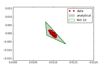
Figure 1: A 2-D projection of Laurberg Data and NVI components. The different components are not distinguishable.

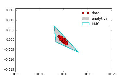
Figure 2: A 2-D projection of Laurberg Data and the components accepted in the HMC + ONVI algorithm. These components are all coming from the same mode, which overlaps with the analytical solution (initialization).

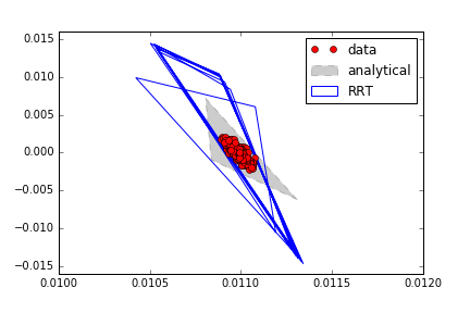
Figure 3: A 2-D projection of Laurberg Data and the components accepted in the RRT + ONVI algorithm. These components are distinct from the analytical solution (initialization). These diverse components continue to explain the data under the Uniform noise model as the data lies in the convex hull of these RRT-based factorizations.

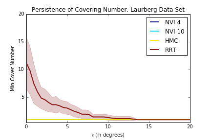
Figure 4: Laurberg Data: A persistence plot of samples from the variational distribution obtained from the different algorithms. The RRT + ONVI is the only algorithm for which minimum cover numbers are larger than one for angles greater than 0.01. The other algorithms are unable to escape the modes that they were initialized in.

5.2 Application to Real Data Sets

We apply our approach to several datasets commonly used for NMF : 20-Newsgroups (Mitchell, 1997) (D=813, N=2034, categories= R = 4); Reuters articles (Lewis, 1987)(D = 1540, N = 2362, categories = R = 4); BBC articles (Greene and Cunningham, 2006)(D = 6045, N = 1162, categories = R = 4); AML/ALL cancer cell data (Žitnik and Zupan, 2012)(D = 5000, N = 38, R = 3) ; Olivetti Faces (Samaria, 1994)(D = 4096, N = 400, R = 4); Hubble telescope hyper-spectral image (Nicolas Gillis, 1987) (D=100, N=4096, R = 8).

RRT+ONVI give comparable or better ELBO values.

Tables 2 and 2 show the ELBO values for our approach compared to the baselines with the noise $\sigma^{2}_{X}$ set to the empirical noise (found by first fitting a solution via Lin’s algorithm and measuring the squared error, before any additional experiments) and 10x this empirical noise. The latter case was designed to simulate a situation where we might expect to see greater variation in solutions.

In both cases, the RRT+ONVI has the highest ELBO across all data sets. However, due to the light tails of the Gaussian distribution, the expectation term (equation 3) dominated the (coverage-encouraging) entropy term (equation 2); all the ONVI variants consistently retained only one highest quality component.

Table 3 shows the results for the Uniform likelihood (similar to before, the noise $\epsilon$ was set based on the absolute deviation from fitting a solution via Lin’s algorithm). Here, the differences between solutions are smaller because they come primarily from differences in the entropy term; thus we show the deviation from the mean ELBO for each data set. As before, the RRT+ONVI finds the variational distribution with the highest ELBO. The HMC+ONVI fails to move significantly from its starting point and thus only retains one component; in contrast the RRT+ONVI retains between 2 (AML) and 118 (BBC) components depending on the data set.

RRT+ONVI has more posterior coverage

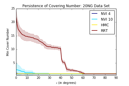
Figure 5: 20-Newsgroups data: Persistence plot of the components shows that RRT + ONVI components are more spread out than baselines.

The evaluations above showed that our RRT+ONVI approach achieves comparable or better ELBO values on real datasets. Now we return to our goal: posterior coverage. Figures 5,  6,  7,  8,  9, and 10 plot the minimum covering number of the components of the variational distribution under the WAD similarity measure. While there is a range of variation across the data sets in terms of angle, the RRT components are most distinctly placed.

Table 1: Empirical Gaussian Noise Setting - We show values of the mean ELBO as well as the 25^th and 75^th percentiles. Across the datasets, the RRT + ONVI procedure finds the best variational fit to the true posterior.

	NVI-4	NVI-10	Gibbs	HMC	RRT
20 Newsgroups	3.115e+06	3.116e+06	3.145e+06	3.151e+06	3.191e+06
	3.115e+06,	3.115e+06,	3.144e+06,	3.150e+06,	3.190e+06,
	3.116e+06	3.117e+06	3.145e+06	3.152e+06	3.191e+06
BBC	2.030e+07	2.030e+07	2.058e+07	2.051e+07	2.061e+07
	2.030e+07,	2.030e+07,	2.057e+07,	2.049e+07,	2.061e+07,
	2.030e+07	2.030e+07	2.058e+07	2.052e+07	2.061e+07
Reuters	8.266e+06	8.266e+06	8.239e+06	8.232e+06	8.276e+06
	8.264e+06,	8.265e+06,	8.235e+06,	8.228e+06,	8.264e+06,
	8.267e+06	8.267e+06	8.243e+06	8.237e+06	8.290e+06
AML	-1.536e+06	-1.536e+06	-1.571e+06	-1.564e+06	-1.510e+06
	-1.536e+06,	-1.536e+06,	-1.571e+06,	-1.565e+06,	-1.510e+06,
	-1.536e+06	-1.536e+06	-1.570e+06	-1.563e+06	-1.510e+06
Faces	1.292e+06	1.293e+06	1.284e+06	1.288e+06	1.314e+06
	1.290e+06,	1.292e+06,	1.281e+06,	1.283e+06,	1.314e+06,
	1.295e+06	1.295e+06	1.288e+06	1.294e+06	1.314e+06
Hubble	-2.593e+07	-8.079e+06	-8.022e+06	-6.179e+07	1.975e+06
	-3.566e+07,	-1.199e+07,	-1.554e+06,	-8.485e+07,	1.959e+06,
	1.988e+06	1.815e+06	4.441e+05	-1.562e+07	1.990e+06

Table 2: Larger Gaussian Noise Setting - We show values of the mean ELBO as well as the 25^th and 75^th percentiles. Across the datasets, the RRT + ONVI procedure finds the best variational fit to the true posterior.

	NVI-4	NVI-10	Gibbs	HMC	RRT
20 Newsgroups	2.298e+05	2.298e+05	1.968e+05	2.050e+05	2.326e+05
	2.297e+05,	2.298e+05,	1.967e+05,	2.049e+05,	2.326e+05,
	2.298e+05	2.299e+05	1.970e+05	2.050e+05	2.327e+05
BBC	7.709e+06	7.712e+06	7.782e+06	7.760e+06	7.844e+06
	7.693e+06,	7.698e+06,	7.781e+06,	7.760e+06,	7.844e+06,
	7.726e+06	7.723e+06	7.782e+06	7.761e+06	7.844e+06
Reuters	1.767e+06	1.767e+06	1.723e+06	1.730e+06	1.768e+06
	1.767e+06,	1.767e+06,	1.723e+06,	1.730e+06,	1.768e+06,
	1.767e+06	1.767e+06	1.724e+06	1.730e+06	1.768e+06
AML	-1.842e+06	-1.842e+06	-1.858e+06	-1.873e+06	-1.818e+06
	-1.843e+06,	-1.842e+06,	-1.859e+06,	-1.874e+06,	-1.818e+06,
	-1.842e+06	-1.842e+06	-1.858e+06	-1.872e+06	-1.818e+06
Faces	-1.644e+06	-1.643e+06	-1.647e+06	-1.643e+06	-1.631e+06
	-1.644e+06,	-1.643e+06,	-1.648e+06,	-1.643e+06,	-1.631e+06,
	-1.644e+06	-1.643e+06	-1.647e+06	-1.642e+06	-1.631e+06
Hubble	7.551e+05	9.657e+05	1.126e+06	6.692e+05	1.208e+06
	8.755e+05,	9.347e+05,	1.119e+06,	8.575e+05,	1.207e+06,
	1.122e+06	1.089e+06	1.136e+06	9.407e+05	1.209e+06

Table 3: Uniform Likelihood: This table shows ELBO deviation from dataset mean and number of RRT components accepted into the ONVI. In all cases, the HMC + ONVI led to unimodal variational distributions. We see that the range of components found are data-set dependent. We provide the mean, first quartile (25) and third quartile (75).

	NVI 4	NVI 10	HMC	RRT	Components (RRT)
20 Newsgroups	-3.080e-01	-1.228e+06	-1.499e+00	1.693e+00	14.8
	-1.708e+00,	-1.228e+06,	-1.708e+00,	1.823e+00,	8,
	3.500e-01	-1.228e+06	-1.360e+00	1.883e+00	21
BBC	-2.780e-01	-3.481e+06	-3.109e+00	3.040e+00	57
	-1.210e+00,	-3.481e+06,	-3.117e+00,	3.035e+00,	29.2,
	9.375e-01	-3.481e+06	-3.103e+00	3.050e+00	77.2
Reuters	-1.840e-01	-2.079e+06	-7.622e-01	1.030e+00	6
	-7.675e-01,	-2.079e+06,	-7.700e-01,	1.030e+00,	6
	6.825e-01	-2.079e+06	-7.600e-01	1.030e+00	6
AML	6.610e-01	-2.216e+06	-2.749e+00	1.430e+00	2
	6.225e-01,	-2.216e+06,	-6.585e+00,	1.430e+00,	2,
	7.275e-01	-2.216e+06	7.025e-01	1.430e+00	2
Faces	-4.580e-01	-8.713e+05	-4.580e-01	1.370e+00	5
	-5.825e-01,	-8.713e+05,	-5.825e-01,	1.370e+00,	5,
	-2.800e-01	-8.713e+05	-2.800e-01	1.370e+00	5
Hubble	-5.389e-01	-1.563e+05	-5.389e-01	1.620e+00	3
	-1.170e+00,	-1.563e+05,	-1.170e+00,	1.620e+00,	3,
	-3.800e-01	-1.563e+05	-3.800e-01	1.620e+00	3

In particular, the persistence plots that for datasets such as 20-Newsgroups and BBC have a lot of variation in the number of modes found and some variation in how the persistence curve drops to 1 as angle gets larger. This variation is indicative of the random nature of the RRT across different repetitions of the experiment. In the remaining datasets we see much less variation. It appears that the ONVI has consistently accepted components from the random restarts of Lin’s algorithm (in the initialization of the RRT). In the case of AML and Faces datasets, the RRT finds multiple components for the ONVI to consider but the ONVI rejects them based on the entropy-based ELBO improvement criteria. In the Reuters and Hubble datasets, the RRT fails to expand from the initial base nodes.

6 Discussion

Our rapid posterior exploration approach involved making many choices, ranging from the approximating variational family to the exploration properties of the RRT. First and foremost, we observed that the the choice of the likelihood model plays a crucial role in determining the shape of the posterior—obvious, perhaps, but not necessarily observable if one’s algorithms limit the posterior approximation to small regions. The noise parameters can also have large effects. For consistency, in our experiments we set $\epsilon$ in the Uniform likelihood as the largest absolute deviation between the data and NMF approximation based on ten random restarts of Lin’s algorithm. However, in other experiments, we found increasing $\epsilon$—to $\epsilon_{\text{new}}=2\epsilon$ for Faces, $\epsilon_{\text{new}}=8\epsilon$ for Hubble—resulted in many more components in the posterior contructed by ONVI. It may be more appropriate to specify $\epsilon_{i,j}$ for each entry $i,j$ in the data $X$.

The isotropic variance of our variational family is restrictive. For high-density regions of the Bayesian NMF posterior, we can expect a perturbation of the basis matrix to be correlated to an appropriate change in the weights matrix. A mixture of Gaussians with more general covariances might therefore be most appropriate. For such a model, Huber et al. (2008) describe a generalization of the lower bound of the entropy formula that we used in equation 2. The question of determining the entries of the covariance matrices would need some insight. Simply trying to optimize for the entries in the covariance matrix would make the problem high-dimensional again as each step in the ONVI would involve solving for a covariance matrix of a $R(D+N)-$dimensional vector.

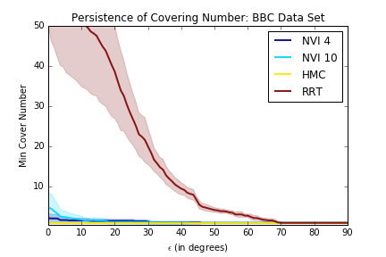
Figure 6: BBC data: Persistence plot of the components shows that RRT + ONVI components are more spread out than baselines.

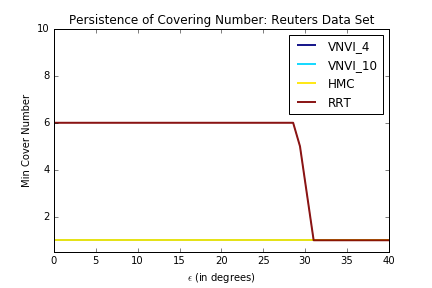
Figure 7: Reuters data: Persistence plot of the components shows that RRT + ONVI components are more spread out than baselines.

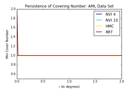
Figure 8: AML/ALL data: The RRT + ONVI components are more spread out than baselines but it is a much smaller spread in terms of angle. For angles greater than 0.1 the minimum covering number is one for all algorithms.

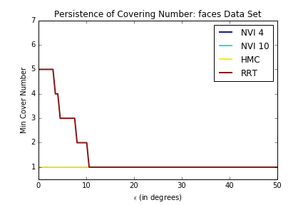
Figure 9: Faces data: The RRT + ONVI components are spread out more than baselines.

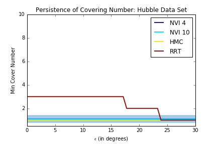
Figure 10: Hubble data: The RRT + ONVI components show the largest posterior coverage.

The ONVI serves to accept/reject candidate components and to adjust accepted components within the variational posterior in an optimal manner. Before introducing candidate components to the ONVI, one might also imagine using a diversification strategy such as hard-core processes or determinental point processes Kulesza and Taskar (2012) to cull the set of candidate nodes. Such a step could help eliminate redundant candidate nodes and reduce the number of candidate nodes presented to the ONVI.

Lastly, there were many parameter choices made in the initialization and expansion of the RRT. Changing the RRT parameters can make a difference in the posterior constructed by the ONVI. For example, the RRT fails to expand in the Reuters dataset (under the Uniform likelihood) using our default parameters, but we noticed that increasing the initial step-size from $s_{0}=0.01$ to $s_{0}=0.5$ allows the RRT to expand and contribute new components to the posterior constructed by the ONVI. An interesting future direction is to adapt the RRT to specific noise-models and datasets. To allow for a larger number of temporary and base nodes (to aid the RRT expansion) we suggest using more efficient data structures for finding the nearest point in the tree (Atramentov and LaValle, 2002). For exploring posterior regions that are not conducive to RRT expansion, alternative exploratory techniques such as probabilistic road maps (Kavraki et al., 1996) can be employed.

7 Related Work

Outside of the empirical work of Greene et al. (2008) and Roberts et al. (2016), we are not aware of work that has been done to to explicitly consider multiple modes (or connected posterior regions) in NMF. In the Bayesian setting, there have been several general approaches to encourage samplers to explore and mix between modes. Neal et al. (2011) discusses a specific approach to tempering in HMC; Green and Mira (2001) discusses an MH approach that delays rejections to allow a far-reaching proposal to find an alternate mode. Sminchisescu et al. (2007) describe approaches for hopping between modes if the locations of the modes are known to the sampler in advance. Both simulated (Marinari and Parisi, 1992) and parallel (Hansmann, 1997) tempering methods are popular for encouraging samplers to move to new regions of high posterior density. Wang-Landau sampling (Schulz et al., 2003) is a popular MCMC sampling method in statistical physics that involves a random walk in the energy space rather than sampling at a fixed temperature.

Within variational methods, mean-field approaches (Beal, 2003; Jordan et al., 1999) are popular but limited to approximating posteriors with unimodal distributions. The use of mixture distributions in mean-field approaches (Lawrence and Jordan, 1998; Jaakkola and Jordan, 1998; Bouchard and Zoeter, 2009) adds flexibility to the posterior but the parameter updates are model dependent and may be difficult to derive. We choose a Gaussian mixture with isotropic variance for our variational family. This is a special case of the mixture mean-field approach for which the inference algorithm provided by (Gershman et al., 2012) can be used for a more general class of models as only knowing the joint likelihood and its gradient is required. Flow-based methods of creating flexible posterior families (such as Non-linear Independent Components Estimation (Dinh et al., 2014) and Hamiltonian variational approximation (Salimans et al., 2015) use a series of functions that transform the parameter space. The normalizing flows framework unifies and presents a generalization of these flow-based variational methods for flexible posteriors (Rezende and Mohamed, 2015)

More broadly, the problem of locating multiple modes or a frontier of solutions has been studied in the optimization literature, though not for the particular case of NMF. Many of these approaches are particle or swarm approaches, in which multiple solutions are initialized, adjusted, and killed according to some evolution and fitness function (e.g. Dorsey and Mayer (1995); Brits et al. (2007). In some cases, explicit rules are made for finding solutions that are in alternate modes (Wales and Doye, 1997). Homotopy methods are used to explore the Pareto surface of nonlinear functions (Das and Dennis, 1998).

In some work, NMF is specifically used for clustering data. Greene et al. (2008) and Huang et al. (2011) use ensemble NMF techniques to understand the space of clusterings obtained through distinct NMF solutions (obtained from random restarts of NMF alogirthms). More work exists for finding multiple alternate clusterings, which can be viewed as a subset of matrix factorizations in which each observation is associated with only one latent feature. Niu et al. (2010) iteratively find multiple clustering views by taking advantage of relationships between the spectral clustering objective and the Hilbert-Schmidt Independence Criterion. Qi and Davidson (2009) apply constrained optimization that defines trade-offs between alternativeness and clustering quality, also separate into finding a single alternative and multiple alternatives, while Gondek and Hofmann (2007) use a mutual information-based criterion to subtract out the information from existing alternatives to propose new ones. Finally, Grimmer and King (2011) simply run a large number of different clustering algorithms and display the alternatives.

To our knowledge, our application of explicit exploration algorithms for posterior coverage is novel.

8 Conclusion

In this work, we leveraged some key geometric insights about NMF to first create a smaller search space, applied RRTs to explore this space, and incorporated these nodes into a flexible, more complete posterior via the nonparametric variational inference framework. Importantly, only the design of the RRT using the oblique manifold is specific to NMF: we expect that this notion of casting posterior inference as an explicit exploration problem will be fruitful for many other models as well.

Acknowledgements

We thank Andrew Miller, Wei Wei Pan, and Michael Hughes for insightful discussions. This work was supported by Defense Advanced Research Projects Agency (DARPA) grant number W911NF-16-1-0561.

References

- Greene et al. [2008] Derek Greene, Gerard Cagney, Nevan Krogan, and Pádraig Cunningham. Ensemble non-negative matrix factorization methods for clustering protein–protein interactions. Bioinformatics, 2008.
- Roberts et al. [2016] Margaret E Roberts, Brandon M Stewart, and Dustin Tingley. Navigating the local modes of big data. Computational Social Science, page 51, 2016.
- Brunet et al. [2004] Jean-Philippe Brunet, Pablo Tamayo, Todd R Golub, and Jill P Mesirov. Metagenes and molecular pattern discovery using matrix factorization. PNAS, 101(12):4164–4169, 2004.
- Paisley et al. [2015] John Paisley, David M Blei, and Michael I Jordan. Bayesian nonnegative matrix factorization with stochastic variational inference. Handbook of Mixed Membership Models and Their Applications. Chapman and Hall/CRC, 2015.
- Schmidt et al. [2009] Mikkel N Schmidt, Ole Winther, and Lars Kai Hansen. Bayesian non-negative matrix factorization. In Independent Component Analysis and Signal Separation, pages 540–547. Springer, 2009.
- Moussaoui et al. [2006] Saïd Moussaoui, David Brie, Ali Mohammad-Djafari, and Cédric Carteret. Separation of non-negative mixture of non-negative sources using a bayesian approach and mcmc sampling. Signal Processing, IEEE Transactions on, 54(11):4133–4145, 2006.
- Lin [2007] Chih-Jen Lin. Projected gradient methods for nonnegative matrix factorization. Neural computation, 19(10):2756–2779, 2007.
- Lee and Seung [2001] Daniel D Lee and H Sebastian Seung. Algorithms for non-negative matrix factorization. In Advances in neural information processing systems, pages 556–562, 2001.
- Recht et al. [2012] Ben Recht, Christopher Re, Joel Tropp, and Victor Bittorf. Factoring nonnegative matrices with linear programs. In Advances in Neural Information Processing Systems, pages 1214–1222, 2012.
- Pan and Doshi-Velez [2016] Weiwei Pan and Finale Doshi-Velez. A characterization of the non-uniqueness of nonnegative matrix factorizations. arXiv preprint arXiv:1604.00653, 2016.
- Donoho and Stodden [2003] David Donoho and Victoria Stodden. When does non-negative matrix factorization give a correct decomposition into parts? In Advances in neural information processing systems, page None, 2003.
- Arora et al. [2012] Sanjeev Arora, Rong Ge, Ravindran Kannan, and Ankur Moitra. Computing a nonnegative matrix factorization–provably. In Proceedings of the forty-fourth annual ACM symposium on Theory of computing, pages 145–162. ACM, 2012.
- Ge and Zou [2015] Rong Ge and James Zou. Intersecting faces: Non-negative matrix factorization with new guarantees. In International Conference on Machine Learning, page X. ICML, 2015.
- Bhattacharyya et al. [2016] Chiranjib Bhattacharyya, IISC ERNET, Navin Goyal, COM Ravindran Kannan, and COM Jagdeep Pani. Non-negative matrix factorization under heavy noise. In Proceedings of The 33rd International Conference on Machine Learning, pages 1426–1434, 2016.
- Hoffman and Blei [2015] Matthew D Hoffman and David M Blei. Structured stochastic variational inference. In Artificial Intelligence and Statistics, 2015.
- Masood et al. [2016] Arjumand Masood, Weiwei Pan, and Finale Doshi-Velez. An empirical comparison of sampling quality metrics: A case study for bayesian nonnegative matrix factorization. CoRR, abs/1606.06250, 2016. URL http://arxiv.org/abs/1606.06250.
- Gershman et al. [2012] Samuel J Gershman, Matthew D Hoffman, and David M Blei. Nonparametric variational inference. 2012.
- Ranganath et al. [2014] Rajesh Ranganath, Sean Gerrish, and David M Blei. Black box variational inference. In AISTATS, pages 814–822, 2014.
- LaValle [1998] Steven M LaValle. Rapidly-exploring random trees: A new tool for path planning. 1998.
- Laurberg et al. [2008] H. Laurberg, M. Christensen, M. Plumbley, L. Hansen, and S. Jensen. Theorems on positive data: on the uniqueness of nmf. Computational Intelligence and Neuroscience, 2008.
- Ročková and George [2015] Veronika Ročková and Edward I George. Fast bayesian factor analysis via automatic rotations to sparsity. Journal of the American Statistical Association, 2015.
- Absil et al. [2009] P-A Absil, Robert Mahony, and Rodolphe Sepulchre. Optimization algorithms on matrix manifolds. Princeton University Press, 2009.
- Kuffner and LaValle [2000] James J Kuffner and Steven M LaValle. Rrt-connect: An efficient approach to single-query path planning. In Robotics and Automation, 2000. Proceedings. ICRA’00. IEEE International Conference on, volume 2, pages 995–1001. IEEE, 2000.
- Neal et al. [2011] Radford M Neal et al. Mcmc using hamiltonian dynamics. Handbook of Markov Chain Monte Carlo, 2:113–162, 2011.
- [25] Dougal Maclaurin, David Duvenaud, and Ryan P Adams. Autograd: Effortless gradients in numpy.
- Mitchell [1997] Tom Mitchell. UCI machine learning repository: Twenty newsgroups, 1997. URL https://archive.ics.uci.edu/ml/datasets/Twenty+Newsgroups.
- Lewis [1987] David D. Lewis. UCI machine learning repository: Reuters-21578, 1987. URL http://archive.ics.uci.edu/ml/datasets/reuters-21578+text+categorization+collection.
- Greene and Cunningham [2006] Derek Greene and Pádraig Cunningham. Practical solutions to the problem of diagonal dominance in kernel document clustering. In ICML, pages 377–384. ACM, 2006.
- Žitnik and Zupan [2012] Marinka Žitnik and Blaž Zupan. Nimfa: A python library for nonnegative matrix factorization. The Journal of Machine Learning Research, 13(1):849–853, 2012.
- Samaria [1994] Ferdinando S. Samaria. The database of faces (olivetti), 1994. URL http://www.cl.cam.ac.uk/research/dtg/attarchive/facedatabase.html.
- Nicolas Gillis [1987] Robert J. Plemmons Nicolas Gillis. Hubble telescope hyperspectral image data, 1987. URL https://sites.google.com/site/nicolasgillis/code.
- Huber et al. [2008] Marco F Huber, Tim Bailey, Hugh Durrant-Whyte, and Uwe D Hanebeck. On entropy approximation for gaussian mixture random vectors. In Multisensor Fusion and Integration for Intelligent Systems, 2008. MFI 2008. IEEE International Conference on, pages 181–188. IEEE, 2008.
- Kulesza and Taskar [2012] Alex Kulesza and Ben Taskar. Determinantal point processes for machine learning. arXiv preprint arXiv:1207.6083, 2012.
- Atramentov and LaValle [2002] Anna Atramentov and Steven M LaValle. Efficient nearest neighbor searching for motion planning. In Robotics and Automation, 2002. Proceedings. ICRA’02. IEEE International Conference on, volume 1, pages 632–637. IEEE, 2002.
- Kavraki et al. [1996] Lydia E Kavraki, Petr Svestka, J-C Latombe, and Mark H Overmars. Probabilistic roadmaps for path planning in high-dimensional configuration spaces. IEEE transactions on Robotics and Automation, 12(4):566–580, 1996.
- Green and Mira [2001] Peter J Green and Antonietta Mira. Delayed rejection in reversible jump metropolis–hastings. Biometrika, 88(4):1035–1053, 2001.
- Sminchisescu et al. [2007] Cristian Sminchisescu, Max Welling, and G Hinton. Generalized darting monte carlo. In AISTATS, pages 516–523. Citeseer, 2007.
- Marinari and Parisi [1992] Enzo Marinari and Giorgio Parisi. Simulated tempering: a new monte carlo scheme. EPL (Europhysics Letters), 19(6):451, 1992.
- Hansmann [1997] Ulrich HE Hansmann. Parallel tempering algorithm for conformational studies of biological molecules. Chemical Physics Letters, 281(1):140–150, 1997.
- Schulz et al. [2003] BJ Schulz, K Binder, M Müller, and DP Landau. Avoiding boundary effects in wang-landau sampling. Physical Review E, 67(6):067102, 2003.
- Beal [2003] Matthew James Beal. Variational algorithms for approximate Bayesian inference. University of London London, 2003.
- Jordan et al. [1999] Michael I Jordan, Zoubin Ghahramani, Tommi S Jaakkola, and Lawrence K Saul. An introduction to variational methods for graphical models. Machine learning, 37(2):183–233, 1999.
- Lawrence and Jordan [1998] Christopher M Bishop Neil Lawrence and Tommi Jaakkola Michael I Jordan. Approximating posterior distributions in belief networks using mixtures. In Advances in Neural Information Processing Systems 10: Proceedings of the 1997 Conference, volume 10, page 416. MIT Press, 1998.
- Jaakkola and Jordan [1998] Tommi S Jaakkola and Michael I Jordan. Improving the mean field approximation via the use of mixture distributions. In Learning in graphical models, pages 163–173. Springer, 1998.
- Bouchard and Zoeter [2009] Guillaume Bouchard and Onno Zoeter. Split variational inference. In Proceedings of the 26th Annual International Conference on Machine Learning, pages 57–64. ACM, 2009.
- Dinh et al. [2014] Laurent Dinh, David Krueger, and Yoshua Bengio. Nice: Non-linear independent components estimation. arXiv preprint arXiv:1410.8516, 2014.
- Salimans et al. [2015] Tim Salimans, Diederik P Kingma, Max Welling, et al. Markov chain monte carlo and variational inference: Bridging the gap. In International Conference on Machine Learning, pages 1218–1226, 2015.
- Rezende and Mohamed [2015] Danilo Jimenez Rezende and Shakir Mohamed. Variational inference with normalizing flows. arXiv preprint arXiv:1505.05770, 2015.
- Dorsey and Mayer [1995] Robert E Dorsey and Walter J Mayer. Genetic algorithms for estimation problems with multiple optima, nondifferentiability, and other irregular features. J of Business & Economic Statistics, 13(1):53–66, 1995.
- Brits et al. [2007] R Brits, Andries Petrus Engelbrecht, and Frans van den Bergh. Locating multiple optima using particle swarm optimization. Applied Mathematics and Computation, 189(2):1859–1883, 2007.
- Wales and Doye [1997] David J Wales and Jonathan PK Doye. Global optimization by basin-hopping and the lowest energy structures of lennard-jones clusters containing up to 110 atoms. The Journal of Physical Chemistry A, 101(28):5111–5116, 1997.
- Das and Dennis [1998] Indraneel Das and John E Dennis. Normal-boundary intersection: A new method for generating the pareto surface in nonlinear multicriteria optimization problems. SIAM Journal on Optimization, 8(3):631–657, 1998.
- Huang et al. [2011] Xiaodi Huang, Xiaodong Zheng, Wei Yuan, Fei Wang, and Shanfeng Zhu. Enhanced clustering of biomedical documents using ensemble non-negative matrix factorization. Information Sciences, 181(11):2293–2302, 2011.
- Niu et al. [2010] Donglin Niu, Jennifer G Dy, and Michael I Jordan. Multiple non-redundant spectral clustering views. In Proceedings of the 27th international conference on machine learning (ICML-10), pages 831–838, 2010.
- Qi and Davidson [2009] ZiJie Qi and Ian Davidson. A principled and flexible framework for finding alternative clusterings. In Proceedings of the 15th ACM SIGKDD international conference on Knowledge discovery and data mining, pages 717–726. ACM, 2009.
- Gondek and Hofmann [2007] David Gondek and Thomas Hofmann. Non-redundant data clustering. Knowledge and Information Systems, 12(1):1–24, 2007.
- Grimmer and King [2011] Justin Grimmer and Gary King. General purpose computer-assisted clustering and conceptualization. PNAS, 108(7):2643–2650, 2011.