A hybrid particle-continuum resolution method and its application to a homopolymer solution

Abstract

We discuss in detail a recently proposed hybrid particle-continuum scheme for complex fluids and evaluate it at the example of a confined homopolymer solution in slit geometry. The hybrid scheme treats polymer chains near the impenetrable walls as particles keeping the configuration details, and chains in the bulk region as continuous density fields. Polymers can switch resolutions on the fly, controlled by an inhomogeneous tuning function. By properly choosing the tuning function, the representation of the system can be adjusted to reach an optimal balance between physical accuracy and computational efficiency. The hybrid simulation reproduces the results of a reference particle simulation and is significantly faster (about a factor of 3.5 in our application example).

I Introduction

In materials science, one often encounters situations where the relevant properties of a material are crucially influenced by the local microstructure at certain localized regions in space, whereas almost everywhere else, in the “bulk”, the specific structure only matters in an average sense. For example, details of the local structure at surfaces are more important for many applications than details of the bulk structure polymer_surface . Other prominent examples are nanocomposites, where the behavior of a material can be improved or even completely changed by filling it with small quantities of additives nc1 ; nc2 ; nc3 ; protein-particle ; nc4 ; nc5 . For a physical modelling of such composites, a finer description of the additives, e.g., at the atomistic level or even quantum level, is necessary, while a coarser grained description of the remaining medium, e.g., at a coarse-grained particle level or continuum level, is often sufficient. This clearly calls for multiscale hybrid simulation approaches.

Multiscale hybrid modelling is a challenging and rapidly developing field in the communities of condensed matter physics, materials science, and engineering QMMM1 ; QMMM2 ; atom-coarse ; EEL07 ; Multi_FT ; AA_CG ; lockerby . One prominent early example is the quantum mechanics (QM)/molecular dynamics (MD) scheme QMMM2 , where small (e.g., chemically reacting) regions are treated at a quantum mechanical level and the environment by classical molecular dynamics. Whereas particles cannot move from one resolution region to another in the QM/MM scheme, the recently developed adaptive resolution schemes (AdResS) review ; adaptive allow for free diffusion of particles and connect different resolution regions in space by means of smooth interpolation functions adaptive ; potential ; Lagrange . AdResS schemes have been proposed that combine the hybrid atomistic/coarse grained scales AandC and the quantum/coarse grained scales CandQ ; Poma . However, these methods are restricted to particle-based simulation models.

On large scales, continuum descriptions which disregard microscopic details (e.g., elastic models, phase field models, hydrodynamic models) are often favorable, since they work with collective variables that directly reflect the relevant mesoscopic properties of a material. Hence hybrid multiscale schemes that couple small-scale particle-based descriptions to large-scale continuous descriptions are of particular interest. One relatively straightforward approach is to permanently treat certain components of a system as particles immersed in a continuous medium IB_1 ; IB_2 ; BD_FTS ; DPD_PF . Another increasingly popular type of approach is concurrent particle/field modeling, where particle simulations are used to determine the dynamical evolution of a continuum model. Prominent examples are the heterogeneous multiscale method EEL07 ; lockerby ; HMM_01 , which uses particle simulations to adjust the rheological parameters of a hydrodynamic continuum model on the fly, and “Single chain in Mean Field” simulation methods BD_DSCF ; SCF_BD_A1 ; SCMF1 ; SCMF2 ; SCF_MD1 ; SCF_MD2 ; SCF_MD3 , where simulations of instantaneously uncorrelated chains are used to determine the dynamical evolution of fields in a dynamic density functional. However, few methods exist that allow to “zoom into” certain particle-resolved regions in space within a continuum simulation in an adaptive resolution sense. One such scheme was developed by Delgado-Buscalioni, de Fabritiis, and coworkers particle_NS ; particle_FH ; MD_FHM ; triple . It can be applied to simple or molecular fluids and couples molecular dynamics simulations of fluids with the fluctuating Navier-Stokes equations fluctuation_hydrodynamics through a hybrid interfacial region. Another scheme which allows one to construct adaptive resolution models for soft materials in a formally exact manner was recently proposed by us Hybrid_PF . The purpose of the present paper is to discuss possible implementations and variants of this approach and to evaluate it systematically at the example of a simple model system, a confined homopolymer solution.

The construction of our hybrid scheme starts from particle resolution (PR) models of the Edwards type Edwards , in which the interactions are expressed in terms of local densities. Edwards type models are popular starting points in theoretical polymer physics BD_DSCF2 ; RPA ; GaussianApprox ; variational ; renormalization and are often used for the interpretation of experimental phenomena in soft matter and biophysics, as well as for efficient particle-based computer simulations Edwards01 ; Edwards02 ; Edwards03 ; Hans ; brush_switch . In our adaptive resolution approach, we exploit the fact that the partition function of Edwards models can be rewritten exactly as a fluctuating field theory. Hence each Edwards particle model has a continuum partner, and our scheme relies on the equivalence between the particle model and its continuum partner. This allows one to single out selected regions in space to be treated at a particle level within a field-based continuum simulation.

We note that similar field theoretical mappings to continuous models can also be performed for other particle models, as long as particles do not interact with hard core interactions. Our scheme is not limited to Edwards models. However, the underlying particle must be coarse-grained in the sense that particle interactions are soft (or of Coulomb type). In the present paper, we will specifically consider the simplest Edwards type model, which describes homopolymer solutions in an implicit solvent. This model already contains basic ingredients of soft matter systems, i.e., the competition of entropy and interaction energy and the tunable and relatively large length scales which characterize soft systems.

We construct the hybrid adaptive resolution scheme following the basic idea sketched in Ref. Hybrid_PF , focussing on an implicit solvent system. We explain in detail the construction and implementation of the hybrid scheme, and evaluate the computational efficiency of the present scheme by comparison with its pure particle-based counterpart. We hope that the present work will help other researchers to implement the hybrid scheme. The paper is organized as follows. In Sec. 2, the hybrid model is derived, and numerical algorithms that can be applied in practical simulations are discussed. Results for the confined homopolymer solution are presented in Sec. 3. We summarize and conclude in Sec. 4.

II Hybrid particle-continuum resolution model

In this section, we present the basic methodology of the hybrid particle-field simulation approach. For simplicity, we consider the simple system of a homopolymer solution in an implicit solvent. Generalizations to other soft matter systems are straightforward.

II.1 Construction of the particle-continuum adaptive resolution method

Let us consider a collection of $n_{t}$ polymers in a three-dimensional volume $V$. The polymers are modeled as linear chains of $N$ beads connected by Gaussian springs GausianChain with a spring constant $\frac{3}{b^{2}}$, where we set $k_{B}T\equiv 1$ ($k_{B}$ is the Boltzmann constant, $T$ the temperature) and $b^{2}$ is the mean-squared bond length. Throughout this paper, we will measure lengths in units of the radius of the gyration of the ideal chain, $R_{g}=\sqrt{\frac{Nb^{2}}{6}}$, hence $b^{2}=\frac{6}{N}$. The energy of the system is expressed as an Edwards Hamiltonian offlattice :

$$\mathcal{H}=\frac{V}{n_{t}}\frac{N}{4}\sum_{\alpha=1}^{n_{t}}\sum_{j=1}^{N-1}\Big{[}\mathbf{R}_{\alpha}^{j}-\mathbf{R}_{\alpha}^{j-1}\Big{]}^{2}+\frac{v_{0}}{2}\int d\mathbf{r}\hat{\phi}^{2}_{t}(\mathbf{r}),$$ (1)

where $\mathbf{R}_{\alpha}^{j}$ is the position of the $j$-th bead on the $\alpha$-th polymer. The quantity $\hat{\phi}_{t}(\mathbf{r})$ is the normalized density defined as the microscopic bead density profile $\hat{\rho}_{t}(\mathbf{r})=\sum_{\alpha=1}^{n_{t}}\sum_{j=0}^{N-1}\delta(\mathbf{r}-\mathbf{R}_{\alpha}^{j})$ divided by the average bead density $\rho_{0}=\frac{n_{t}N}{V}$. Since the density is defined from the bead positions, the fundamental particle degrees of freedom are fully resolved in (1). The first term in the Hamiltonian (1) describes the probability distribution of a Gaussian chain. The second term accounts for the effective interaction between beads, and $v_{0}>0$ is the excluded volume parameter. The partition function in the canonical ensemble is given by

$$\mathcal{Z}=\frac{1}{n_{t}!\lambda_{T}^{3n_{t}}}\prod_{\alpha=1}^{n_{t}}\prod_{j=0}^{N-1}\int{\rm d}\mathbf{R}_{\alpha}^{j}\exp\Big{[}-\frac{n_{t}}{V}\mathcal{H}(\{\mathbf{R}\})\Big{]},$$ (2)

where $\lambda_{T}$ is the thermal wavelength accounting for the contribution from kinetic energy. Physical quantities at equilibrium can be extracted from the partition function (2), for instance by Monte Carlo methods Frenkel . It can also serve as the starting point for pure field theoretical simulations.

In the following we recast (2) into an equivalent hybrid particle-field model in a mathematically exact way. The resulting model can then be treated numerically, thus combining the advantages of particle based Monte Carlo techniques and field theoretical simulations. This will be achieved in three steps: (i) The chains will be divided into two virtual species in such a way that the physics is unchanged. (ii) The two species will then be treated by different representations, i.e., one species is still described by beads whereas the second species will be described by fields. (iii) The field representations will then be simplified by adopting approximations that make a numerical treatment more feasible.

In the first step the identical chains of the system are partitioned into two species which we call p-chain and f-chain. This can be done in several ways. The strategy we adopt in the following introduces additional “spin” variables $\tau_{\alpha j}$ for all the beads, each of which takes the values 1 or 0, and a spatially varying conjugate “potential” $\Delta\mu({\bf r})$ which couples to the spin of a bead at position ${\bf r}$. The $\alpha$-th chain is defined to be an f-chain if all $\tau_{\alpha j}$ are 0, otherwise it is a p-chain. The potentials $\Delta\mu$ thus lead to a partitioning into $n_{p}$ and $n_{f}$ chains of p- and f-type. Hereafter, we refer to $\Delta\mu$ as the tuning function (TF). The introduction of the partitioning and of the TF must not change the physics of the system. This is technically achieved by introducing the identities

$$\sum_{\tau_{\alpha j}=0}^{1}{\rm e}^{\big{[}\Delta\mu(\mathbf{R}_{\alpha}^{j})\tau_{\alpha j}-\ln(e^{\Delta\mu(\mathbf{R}_{\alpha}^{j})}+1)\big{]}}=1,$$ (3)

which are valid for each bead $j$ on each chain $\alpha$. Inserting these identities into the partition function (2), we get

$$\mathcal{Z} = \frac{1}{n_{t}!\lambda_{T}^{3n_{t}}}\int\prod_{\alpha=1}^{n_{t}}\prod_{j=0}^{N-1}\sum_{\tau_{\alpha j}=0}^{1}{\rm d}\mathbf{R}_{\alpha}^{j}\>$$ (4)

$$\times\>{\rm e}^{\big{[}\sum_{\beta k}\big{(}\Delta\mu(\mathbf{R}_{\beta}^{k})\tau_{\beta k}-\ln(e^{\Delta\mu(\mathbf{R}_{\beta}^{k})}+1)\big{)}-\mathcal{H}(\{\mathbf{R}\})\big{]}}.$$

By construction, this partition function is equivalent to the original partition function (2), but the artificial variables $\tau_{\alpha j}$ introduce two different types of chains, and an inhomogeneous TF will generate an inhomogeneous partitioning in space. This, however, does not change the physics of the system. By adjusting the form of $\Delta\mu(\mathbf{r})$, one can manipulate the individual density distribution for p-chains and f-chains. For example, larger values of $\Delta\mu(\mathbf{r})$ in some regions will result in higher densities of p-chains in these regions, while smaller values of $\Delta\mu(\mathbf{r})$ will result in higher density of f-chains. By construction the sums of the densities for p-chains and f-chains are the same independent of the choice of $\Delta\mu(\mathbf{r})$ and are identical to the ones obtained directly from (2).

In the partitioning scheme discussed above, $p$-chains and $f$-chains have a very different entropy in spin space: A p-chain can support $2^{N}-1$ possible combinations of spin variables, while only one spin combination is possible in f-chains. To compensate for this asymmetry and achieve $\langle n_{p}\rangle\sim\langle n_{f}\rangle$, the values of the TF must be of order $\Delta\mu_{0}=\ln[2^{1/N}-1]$. Alternative ways to assign virtual identities that avoid this asymmetry are also conceivable. For example, one could attach a spin variable $\tau_{\alpha 0}\in\{0,1\}$ only to the first bead of the $\alpha$-th chain, and declare this chain to be a p- or f-chain if $\tau_{\alpha 0}=1$ or $0$, respectively. In this scheme, the identity (3) is only inserted for beads $j=0$ on chains $\alpha$. The space-dependent tuning function $\Delta\mu$ still determines the spatial distribution of the p- and f-chains and their total numbers $\langle n_{p}\rangle$ and $\langle n_{f}\rangle$, but now the partitioning into p-chains and f-chains is symmetric: The local ratio of f- and p-chains can be exactly reversed by reversing the sign of $\Delta\mu(\mathbf{r})$ and at $\Delta\mu(\mathbf{r})\equiv 0$, the p- and f-chains have the same density distribution. Despite the advantages of such a symmetric scheme, we will use the asymmetric version described earlier, because it treats all beads on the chain on equal footing.

The above construction partitions all chains into either p-chains or f-chains, but they are both still described by particle degrees of freedom. However, we are free to choose other representation methods. One possibility is to describe all the chains by continuum field models. The transition from PR models to field resolution (FR) models can be done in a formally exact way using field theoretic methods (see below), and field-theoretic simulation methods have proved to be powerful tools to investigate the properties of polymeric systemsFTS ; Fredrickson . In the hybrid model, we describe only the f- chains by the FR method and the others still by the PR method. The advantage of such an scheme lies in its ability to exploit and combine the specialties and advantages of different representation schemes simultaneously.

To this end, we first reorder the sum over chains $\alpha$ such that the $p$-chains come first. The conversion of f-chains to a field representation is then done following a standard field-theoretical method, i.e., the fields are introduced through inserting an identity into the partition function Schmid ; SCMF

$$1\propto\int\mathcal{D}W_{f}\mathcal{D}\phi_{f}\exp\left\{\frac{n_{t}}{V}\int d\mathbf{r}\>iW_{f}(\mathbf{r})\Big{[}\phi_{f}(\mathbf{r})-\hat{\phi}_{f}(\mathbf{r})\Big{]}\right\},$$ (5)

where $\hat{\phi}_{f}(\mathbf{r})=\frac{V}{n_{t}N}\sum_{\alpha=n_{p}+1}^{n_{t}}\sum_{j=0}^{N-1}\delta(\mathbf{r}-\mathbf{R}_{\alpha}^{j})$ is the configurational dependent density of all beads belonging to f-chains, $\phi_{f}(\mathbf{r})$ is the fluctuating density field corresponding to these f-chains, and $W_{f}(\mathbf{r})$ is the fluctuating auxiliary field conjugate to the density field. Inserting this identity effectively decouples the particle degrees of freedom of f-chains such that they can be integrated out. Each f-chain then contributes the same factor $Z_{0}\>Q_{f}$ to the partition function, where $Q_{f}$ is the normalized single-chain partition function

$$Q_{f}[iW_{f}]=\frac{1}{Z_{0}}\int d\mathbf{R}_{0}\cdots d\mathbf{R}_{N-1}$$ (6)

$$\times\exp\Big{\{} -\frac{N}{4}\sum\limits_{j=1}^{N-1}(\mathbf{R}_{j}-\mathbf{R}_{j-1})^{2}-\frac{1}{N}\sum\limits_{j=0}^{N-1}iW_{f}[\mathbf{R}_{j}]$$

$$-\>\sum\limits_{j=0}^{N-1}\ln[e^{\Delta\mu(\mathbf{R}_{j})}+1]\Big{\}},$$

(the subscripts $0,\cdots,N-1$ refer to the indices of beads within a chain). The normalization constant $Z_{0}=V\big{(}\frac{N}{4\pi}\big{)}^{3(N-1)/2}$ corresponds to the partition function of an ideal noninteracting reference chain of length $N$ and was introduced to ensure that $Q_{f}$ remains finite in the limit of $N\to\infty$ Fredrickson . The partition function (4) then reads

$$\mathcal{Z} = \frac{1}{n_{t}!\lambda_{T}^{3n_{t}}}\sum_{\{\tau_{\alpha j}\}}\int\mathcal{D}W_{f}(\mathbf{r})\int\mathcal{D}\phi_{f}(\mathbf{r})\prod_{\beta=1}^{n_{p}}\prod_{k=0}^{N-1}\int{\rm d}\mathbf{R}_{\beta}^{k}$$ (7)

$$\times\;\exp\Big{\{}-H_{\tau}-\frac{n_{t}}{V}\mathcal{F}\Big{\}},$$

where the sum $\sum_{\{\tau_{\alpha j}\}}$ runs over all possible spin configurations ($\tau_{\alpha j}=0,1$), the variable $n_{p}$ depends on the spin configuration as explained above, the spin Hamiltonian $H_{\tau}$ is defined by

$$H_{\tau}=-\sum_{\alpha=1}^{n_{t}}\sum_{j=0}^{N-1}\Delta\mu(\mathbf{R}_{\alpha}^{j})\tau_{\alpha j}+\sum_{\alpha=1}^{n_{p}}\sum_{j=0}^{N-1}\ln\Big{[}e^{\Delta\mu(\mathbf{R}_{\alpha}^{j})}+1\Big{]},$$ (8)

and the effective free energy energy functional for polymers $\mathcal{F}$ is given by

$$\mathcal{F}[\{\mathbf{R}_{\alpha}^{j}\},\phi_{f},iW_{f}]=\mathcal{F}_{p}+\mathcal{F}_{f}+\mathcal{F}_{\mathrm{mix}}$$ (9)

with

$$\mathcal{F}_{p} = \frac{V}{n_{t}}\frac{N}{4}\sum_{\alpha=1}^{n_{p}}\sum_{j=1}^{N-1}\Big{[}\mathbf{R}_{\alpha}^{j}-\mathbf{R}_{\alpha}^{j-1}\Big{]}^{2}+\frac{v_{0}}{2}\int d\mathbf{r}\hat{\phi}_{p}^{2}(\mathbf{r})$$

$$\mathcal{F}_{f} = \frac{v_{0}}{2}\int d\mathbf{r}\phi_{f}^{2}(\mathbf{r})-\int d\mathbf{r}\>iW_{f}(\mathbf{r})\phi_{f}(\mathbf{r})$$

$$-\>\frac{Vn_{f}}{n_{t}}\ln Q_{f}[iW_{f}]-\>\frac{Vn_{f}}{n_{t}}\ln Z_{0}$$

$$\mathcal{F}_{\mathrm{mix}} = v_{0}\int d\mathbf{r}\hat{\phi}_{p}(\mathbf{r})\phi_{f}(\mathbf{r}).$$

Here $\mathcal{F}_{p}$ is the Hamiltonian of the pure p-chains, $\mathcal{F}_{f}$ is the free energy of the pure f-chains, and $\mathcal{F}_{\mathrm{mix}}$ is the coupling term. The final expressions (14) of the partition function and (9) for the free energy of a configuration represent our hybrid model which we will further investigate in this article. We note again that there are two kinds of independent degrees of freedom left in the model. One refers to the configurational space which belongs to the PR part, the other is the auxiliary field which belongs to the FR part.

Now we work simultaneously with two kinds of representations, the PR and the FR coexisting in the very same system. Within the PR, polymer chains are characterized by the positions of beads, and the detailed information about configurations is still accessible. Consequently the PR part is referred to as a high resolution representation. The FR of f-chains corresponds to a lower resolution since the configurational information on individual chains is lost, only the continuous density can be observed. The regions in space where the high and the low resolution is adopted are adjusted by the choice of $\Delta\mu$ which governs where the respective representation prevails.

The combined particle-field approach is constructed such that it is formally equivalent to the pure particle model, due to the fact that the field description is introduced by an identity transformation/operator in the partition function. Independent of the choice of the TF, one should obtain the same density distributions for both the pure particle model and the hybrid model. In reality, however, the two models are not truly equivalent, since simulations of the field model inevitably must make approximations. Most importantly, the space must be discretized. This amounts to a regularization of the field theory which is necessary both for obvious practical reasons and for fundamental reasons, to eliminate ultraviolet divergences in the theory katz_05 . The FR model is thus necessarily coarse-grained with a coarse-graining cutoff that is set by the grid size (which gives us one more justification to refer to the FR representation as the “low resolution” representation). We note that the finite cutoff leads to a renormalization of model parameters both in the field theory wang_02 ; kudlay_03 ; morse_07 and in particle simulations with density-based Edwards-type interactions brush_switch (since the density dependent interactions are also evaluated on a grid, see Sec. II.3).

In practical applications of the hybrid model, further approximation may be necessary at the FR level to achieve the desired speedup of the simulation time. They are discussed in the next section.

II.2 Treatment of the field degrees of freedom

The hybrid particle-field model has particle degrees of freedom (the bead positions) and field degrees of freedom (density fields and auxiliary potentials $W$). One difficulty arises from the fact that the free energy functional of the fields $\mathcal{F}_{f}$ (Eq. (9)) becomes complex. Simulations of pure FR models are nevertheless possible with the Complex Langevin technique ComplexLangevin ; FTS , however, they become cumbersome and time consuming. In a hybrid simulation, the Complex Langevin simulation scheme would involve a random walk of all degrees of freedom including the particle degrees of freedom in the whole complex plane. This would seriously affect the PR part of the simulation. In order to avoid that problem, we resort to integrating out some or all field degrees of freedom beforehand within a saddle point approximation. This has the additional advantage that it significantly speeds up the simulations.

One possibility is to carry out the saddle point integration over $W_{f}(\mathbf{r})$ and keep the explicit integral over the ”density” field $\phi_{f}(\mathbf{r})$. Minimizing $\mathcal{F}[\{\mathbf{R}_{\alpha}^{j}\},\phi_{f},iW_{f}]$ with respect to $W_{f}(\mathbf{r})$ gives the following relation

$$\phi_{f}(\mathbf{r}) \stackrel{{\scriptstyle!}}{{=}} -\frac{Vn_{f}}{n_{t}Q_{f}}\frac{\delta Q_{f}}{\delta iW_{f}(\mathbf{r})}\Bigg{|}_{W_{f}^{*}}$$ (10)

$$= \frac{Vn_{f}}{n_{t}}\frac{\sum_{j=0}^{N-1}q_{j}(\mathbf{r})\>q_{N-1-j}(\mathbf{r})}{N\int{\rm d}\mathbf{r}\>q_{0}(\mathbf{r})\>q_{N-1}(\mathbf{r})}$$

between $\phi_{f}(\mathbf{r})$ and the saddle point solution $W_{f}^{*}(\mathbf{r})$. Here $Q_{f}$ is given by Eq. (6) and $q_{j}(\mathbf{r})$ is the end-integrated propagator for a chain, which can be computed via the following recursion relation:

$$q_{0}(\mathbf{r}) = {\rm e}^{-i\frac{1}{2}W_{\mbox{\scriptsize eff}}^{*}(\mathbf{r})}$$ (11)

$$q_{j}(\mathbf{r}) = C{\rm e}^{-\frac{1}{2}iW_{\mbox{\scriptsize eff}}^{*}(\mathbf{r})}\int{\rm d}\mathbf{r}^{\prime}{\rm e}^{-\frac{N}{4}(\mathbf{r}-\mathbf{r}^{\prime})^{2}}{\rm e}^{-\frac{1}{2}iW_{\mbox{\scriptsize eff}}^{*}(\mathbf{r}^{\prime})}\>q_{j-1}(\mathbf{r}^{\prime})$$ (12)

for $$j>0$$

with $C=\sqrt[3]{N/4\pi}$ and $iW_{\mbox{\scriptsize eff}}^{*}:=iW_{f}^{*}+\ln[e^{\Delta\mu}+1]$. Obviously, one has $\int{\rm d}\mathbf{r}\phi_{f}(\mathbf{r})=Vn_{f}/n_{t}$. Furthermore, the single chain partition function (6) can be expressed in terms of the propagator by $Q_{f}=\frac{1}{V}\int{\rm d}\mathbf{r}\>q_{0}(\mathbf{r})\>q_{N-1}(\mathbf{r})$. Since the end-integrated propagators are convolutions, they can be calculated efficiently using fast Fourier transforms. Note that the propagator has been carefully constructed such that all beads, including the end beads, carry the full weight ${\rm e}^{-iW_{\mathrm{eff}}^{*}(\mathbf{r})}$. This is essential especially when considering very short chains. In the continuum approximation the end-integrated propagator satisfies the so called modified diffusion equation Edwards ; Freed

$$\frac{\partial q(\mathbf{r},s)}{\partial s}=\nabla^{2}q(\mathbf{r},s)-iW_{\mbox{\scriptsize eff}}^{*}(\mathbf{r})q(\mathbf{r},s),$$ (13)

with $s\in[0:N]$, which is commonly used in field theoretical simulation models (except for the term $\ln[e^{\Delta\mu}+1]$).

The saddle point integration with respect to the fields $W_{f}$ solves the problem of the complex free energy functional: The saddle field $W_{f}^{*}$ is purely imaginary, hence $iW_{f}^{*}(\mathbf{r})$ is real and the saddle point functional $\mathcal{F}^{*}[\{\mathbf{R}_{\alpha}^{j}\},\phi_{f}]=\mathcal{F}[\{\mathbf{R}_{\alpha}^{j}\},\phi_{f},iW_{f}^{*}]$ becomes real. Nevertheless, the evaluation of $\mathcal{F}^{*}$ for a given configuration of the field $\phi_{f}$ remains cumbersome, since one has to solve the implicit equation Eq. (10) for $iW_{f}^{*}$. To simplify the numerical calculations, we perform a variable transform $\int\mathcal{D}\phi_{f}\to\int\mathcal{D}\omega_{f}$ in the partition function with $\omega_{f}:=iW_{f}^{*}$. This variable transformation is associated with a Jacobian, which can be incorporated in an additional contribution to $F$. However, this contribution is of the same order of magnitude than the leading (Gaussian) fluctuation correction to the saddle point integral, and will be neglected as well. The final expression for the partition function is given by

$$\mathcal{Z} = \frac{1}{n_{t}!\lambda_{T}^{3n_{t}}}\sum_{\{\tau_{\alpha j}\}}\int\mathcal{D}\omega_{f}(\mathbf{r})\prod_{\beta=1}^{n_{p}}\prod_{k=0}^{N-1}\int{\rm d}\mathbf{R}_{\beta}^{k}$$ (14)

$$\times\>\exp\Big{\{}-H_{\tau}-\frac{n_{t}}{V}\mathcal{F}\Big{\}},$$

where $H_{\tau}$ and $\mathcal{F}=\mathcal{F}[\{\mathbf{R}_{\alpha}^{j}\},\phi_{f},\omega_{f}]$ are defined in Eqs. (8) and (9) and $\phi_{f}$ can be calculated from $\omega_{f}$ according to Eq. (10) with $\omega_{f}=iW_{f}$. This summarizes our hybrid model which we will further investigate in this article. We note again that the model operates with two types of independent degrees of freedom: The chain configurational space which belongs to the PR part, and the auxiliary field space which belongs to the FR part.

Alternatively, we can also carry out the saddle point integration with respect to both fluctuating fields, $W_{f}$ and $\phi_{f}$. Hence $\mathcal{F}$ is minimized with respect to both fields, which results in two saddle point equations, Eq. (10) and

$$iW_{f}^{*}(\mathbf{r})=\omega_{f}^{*}(\mathbf{r})\stackrel{{\scriptstyle!}}{{=}}v_{0}\>\big{(}\phi_{f}^{*}(\mathbf{r})+\hat{\phi}_{p}(\mathbf{r})\big{)}.$$ (15)

Within this approximation, fluctuations in the FR part of the model are fully neglected.

II.3 Simulation method

We use the Monte Carlo method Frenkel to sample the remaining degrees of freedom and to calculate statistical averages for the quantities of interest of within the hybrid model. Suitable update moves therefore pertain to the configuration $\{\mathbf{R}_{\alpha}^{j}\}$ of the PR part, the field $\omega_{f}(\mathbf{r})$ of the FR part, and the virtual spin configuration $\{\tau_{\alpha j}\}$.

It is important to note that we must introduce a spatial grid already at the level of the particle model in order to evaluate the density dependent interactions in Eq. (1). The grid and the prescription for calculating the local bead density $\hat{\phi}$ on the grid from a (continuous) chain configuration are part of the definition of the particle model.

Here we split the physical space into small cubic cells whose centers define a grid of points $r_{ijk}$, here, $i,j,k$ denote the index of a grid point. A discretized density p-chain field is then defined on this grid through a “particle-to-mesh” technique PM . For simplicity, we use the “nearest-grid-point” scheme, i.e., $\hat{\phi}_{p}(r_{ijk})$ is defined as the average density in the cell. The definition of the Hamiltonian contains self-interactions. For the near-grid-point scheme, the self-energy is a position independent constant self_energy , and it only shifts the chemical potential. In the present case, this shift can be completely adsorbed in the tuning function and will not affect the statistical averages. The continuous TF is also discretized on the grid: A bead in the cell with center point $r_{ijk}$ is subject to the TF $\Delta\mu(r_{ijk})$. In order to have a consistent definition of collective variables in the FR and PR domains, the field degrees of freedom $\omega(\mathbf{r})$ are discretized on the same grid. However, this is not strictly necessary, and more flexible schemes where the FR grid is much coarser than the PR grid are conceivable.

A simulation starts with an initial configuration $\{\mathbf{R}_{\alpha}^{j}\}$ for $n_{p}$ p-chains and an auxiliary potential $\omega_{f}(\mathbf{r})$ describing the $n_{f}$ f-chains. All p-chains are initially generated as Gaussian chains, and the initial configuration of $\omega_{f}(\mathbf{r})$ can be set randomly. The initial number of $n_{p}$ and $n_{f}$ can be chosen at will, just respecting the total number constraint $n_{p}+n_{f}=n_{t}$. Different starting values will not affect the statistical quantities, but influence the equilibration time of the system. Since the positions of beads and the potential are independent of each other, their respective configurations are updated separately. A Monte Carlo move comprises three steps: (i) The configuration of the p-chains is updated $M_{p}$ times, keeping the potential fixed; (ii) The auxiliary potential of the f-chains is updated $M_{f}$ times, keeping the p-chain configuration fixed; (iii) An identity switch between p- and f-chains is attempted $M_{s}$ times, keeping the configuration of the other chains and the potential fixed. All these trial update steps are accepted according to the Metropolis rule.

i. p-chain update

In updating the p-chain configurations, we randomly select one bead on a randomly chosen p-chain, then move it by a random vector with a length comparable to the bond length. For the end beads, one can also perform reptation moves, meaning that end beads are removed and re-attached to the other end, with a bond vector generated from a Gaussian distribution function with variance given by the squared bond length.

For beads $j$ on chains $\alpha$, trial displacements from the position $\mathbf{R}_{\alpha}^{j}$ to $\tilde{\mathbf{R}}_{\alpha}^{j}$ are accepted with the Metropolis probability

$$P_{p}=\mbox{min}\Bigg{\{}1,\exp\Big{[}-\Delta H_{\tau}-\frac{n_{t}}{V}(\Delta\mathcal{F}_{p}+\Delta\mathcal{F}_{\mbox{\scriptsize mix}})\Big{]}\Bigg{\}},$$ (16)

where $\Delta H_{\tau}=-\Delta\mu(\tilde{\mathbf{R}}_{\alpha}^{j})+\Delta\mu(\mathbf{R}_{\alpha}^{j})+\ln[e^{\Delta\mu(\tilde{\mathbf{R}}_{\alpha}^{j})}+1]+\ln[e^{\Delta\mu(\mathbf{R}_{\alpha}^{j})}+1]$, and $\Delta\mathcal{F}_{p}=\tilde{\mathcal{F}}_{p}-\mathcal{F}_{p}$, $\Delta\mathcal{F}_{\mbox{\scriptsize mix}}=\tilde{\mathcal{F}}_{\mbox{\scriptsize mix}}-\mathcal{F}_{\mbox{\scriptsize mix}}$ are the free energy differences associated with this trial move. In case of the reptation move, $\Delta\mathcal{F}_{p}$ has to exclude the term associated with the bead connectivity (Gaussian spring), since it is already taken into account by the generation of the new bond vector.

ii. f-chain update.

As discussed in Sec. II.2, we perform partial or full saddle point integrations with respect to the field degrees of freedom. This is implemented with the following sampling schemes:

Partial saddle point approximation.

In this case, the “density” degrees of freedom are still fluctuating and our aim is to integrate the partition function (14) by sampling the auxiliary field variables $\omega_{f}$. A simple way to implement this in a Monte Carlo scheme is to generate trial field values by adding a (small) random (positive or negative) number to the old value at each grid point $(ijk)$, e.g.,

$$\tilde{\omega}_{f}(r_{ijk})=\omega_{f}(r_{ijk})+h\cdot a_{ijk}$$ (17)

where the random numbers $a$ are generated uniformly and range from -1 to 1. The magnitude of the constant $h$ affects the equilibration time of the system. The acceptance probability for this move is

$$P_{f}=\mbox{min}\Bigg{\{}1,\exp\Big{[}-\frac{n_{t}}{V}(\Delta\mathcal{F}_{f}+\Delta\mathcal{F}_{\mbox{\scriptsize mix}})\Big{]}\Bigg{\}}$$ (18)

where $\Delta\mathcal{F}_{f}=\tilde{\mathcal{F}}_{f}-\mathcal{F}_{f}$ and $\Delta\mathcal{F}_{\mbox{\scriptsize mix}}$ are the free energy differences associated with this move. Below, we will refer to this potential unbiased algorithm as the PU scheme.

To improve the acceptance rate, one can adopt a potential biased scheme, where the trial displacement vectors $\{a_{ijk}\}$ are biased towards the free energy gradient $\delta F_{f}/\delta\omega_{f}$MC_bias . Unfortunately, the calculation of the gradient in our case is cumbersome: Using the relation $\phi_{f}[\omega_{f}]$ defined by Eq. (10), we can rewrite the gradient as

$$\frac{\delta F_{f}}{\delta\omega_{f}(\mathbf{r})}=\int\>{\rm d}\mathbf{r}^{\prime}\>\frac{\delta F_{f}}{\delta\phi_{f}(\mathbf{r}^{\prime})}\>\frac{\delta\phi_{f}(\mathbf{r}^{\prime})}{\delta\omega_{f}(\mathbf{r})},$$

where $\delta\mathcal{F}/\delta\phi_{f}$ can be obtained easily via

$$\frac{\delta\mathcal{F}}{\delta\phi_{f}(\mathbf{r})}=v_{0}\big{(}\phi_{f}(\mathbf{r})+\hat{\phi}_{p}(\mathbf{r})\big{)}-\omega_{f}(\mathbf{r})=:F(\mathbf{r}),$$ (19)

but $\delta\phi_{f}(\mathbf{r}^{\prime})/\delta\omega_{f}(\mathbf{r})$ is a two-point correlation function Schmid whose exact calculation can be time consuming. Therefore, we use a scheme that biases the trial moves of $\omega_{f}$ in the direction of $\delta\mathcal{F}/\delta\phi_{f}$. This scheme will be denoted PB scheme. Specifically, the trial moves are constructed via

$$\tilde{\omega}_{f}=\omega_{f}+h\cdot\>F+\xi,$$ (20)

where $F$ is given by Eq. (19) and $\xi$ is a random number satisfying $\langle\xi_{n}\rangle=0$ and $\langle\xi_{n}\xi_{n^{\prime}}\rangle=2h$. The priori transition probability from $\omega_{f}$ to $\tilde{\omega}_{f}$ is then given by

$$P^{\mathrm{prior}}_{\omega_{f}\to\omega^{\prime}_{f}}\propto\exp\Big{[}-\frac{\big{(}\tilde{\omega}_{f}-\omega_{f}-h\>F\big{)}^{2}}{4h}\Big{]},$$ (21)

hence auxiliary potentials $\tilde{\omega}_{f}$ that approach the saddle point solution are sampled with higher probability. To recover detailed balance, the acceptance probability for the biased move is evaluated as

$$P_{f}=\min\left\{1,\frac{P^{\mathrm{prior}}_{\tilde{\omega}_{f}\to\omega_{f}}}{P^{\mathrm{prior}}_{\omega_{f}\to\tilde{\omega}_{f}}}\>\exp\big{(}-\Delta\mathcal{F}\big{)}\right\}.$$ (22)

Full saddle point approximation.

In the full saddle point approximation, the potential $\omega_{f}$ is given by $\omega_{f}^{*}$ in Eq. (15), where $\phi_{f}^{*}$ is determined by Eq. (10) with $\omega_{f}^{*}=iW_{f}^{*}$. In order to solve (15) and (10) for $\tilde{\omega}_{f}$ we implement a relaxation scheme based on the evolution equation

$$\frac{d\omega_{f}}{dt}=\frac{\delta\mathcal{F}}{\delta\phi_{f}}=:F.$$ (23)

In discretized form the resulting iterative scheme is given by

$$\omega_{f}^{(n+1)}=\omega_{f}^{(n)}+\Delta t\;F^{(n)},$$ (24)

where $n$ denotes the index of the iteration step, $\Delta t$ is the step length, and $F$ represents the “driving force” for relaxation. The step length should not be set too large, otherwise the iteration does not converge. Usually a few tens of iteration steps are required to reach the fixed point corresponding to the saddle point $\omega_{f}^{*}$. In practice, however, we do not need to know the exact saddle point solution at all times due to the statistical property of the system. Therefore, it is sufficient to perform one or two iteration steps, using the potential obtained in the MC-last step as the initial one. This procedure corresponds to a dynamic density functional scheme (DDFT), where the fields $\omega_{f}$ evolve according to the artificial dynamics (23). If the characteristic time scale of this dynamics is much smaller than the characteristic time scale of the particle dynamics, the fields $\omega_{f}$ adjust to the particle configurations almost adiabatically. The fluctuations of the potential during the simulation reflect the fluctuation of p-chains, and the statistical fluctuations of the field are fully neglected.

iii. Identity switches

The identity switches (i.e. switches between p- and f-chains) are driven by the spin variables on the chain. To change the spin configuration one can randomly choose a bead and randomly update its spin variable, and then determine the resulting species from the new spin configuration Semigrand . As mentioned in subsection II.1, however, a p-chain corresponds to ($2^{N}-1$) possible spin configurations, and an f-chain only to one. Consequently most of the attempted switches will convert a p-chain into a p-chain again and this scheme becomes very inefficient for large $N$. In order to increase the transition probability from p-chains to f-chains, we therefore implement a spin-biased scheme: We first generate a random integer in the interval $[0,n_{p}*M_{\mathrm{mid}}+n_{f})$. If the integer is smaller than $n_{p}*M_{\mathrm{mid}}$, a p-chain is picked, otherwise, an f-chain is chosen. If a p-chain is picked, we randomly choose a bead on one of the $n_{p}$ p-chains, and then flip the spin variable of this bead with a Metropolis acceptance probability. Here $M_{\mathrm{mid}}$ is an arbitrary integer, which we typically choose equal to the number $N$ of beads in a chain, and this bias scheme amounts to attempting $M_{\mbox{\scriptsize mid}}$ times more spin flips on p-chains than on f-chains.

We first consider the case where a spin flip is attempted on an f-chain $\alpha$. By definition, all spin variables on this chain are zero before the flip. If one variable $\tau_{\alpha j}$ is flipped to $\tau_{\alpha j}=1$, the f-chain is eliminated from the system so that the f-chain density becomes $\tilde{\phi}_{f}(\mathbf{r})=\frac{n_{f}-1}{n_{f}}\phi_{f}(\mathbf{r})$ (the potential $\omega_{f}(\mathbf{r})$ is kept fixed), and a new p-chain configuration is generated with bond vectors distributed according to a Gaussian with a variance given by the squared bond length. The priori probability for generating a given chain configuration $\{\mathbf{R}_{\alpha}^{j}\}$ is thus given by $P_{\mathrm{prior}}\propto\exp\big{(}-\frac{n_{t}}{V}\mathcal{F}_{g}[\{\mathbf{R}_{\alpha}^{j}\}]\big{)}$ with

$$\mathcal{F}_{g}[\{\mathbf{R}_{\alpha}^{j}\}]=\frac{V}{n_{t}}\frac{N}{4}\sum_{\alpha j}(\mathbf{R}_{\alpha}^{j}-\mathbf{R}_{\alpha}^{j-1})^{2}-\frac{V}{n_{t}}\ln\mathcal{Z}_{0}.$$ (25)

The Metropolis acceptance rate for this switch must be chosen

$$P_{fp} = \mathrm{min}\Bigg{\{}1,\exp\Big{[}\Delta\mu(\mathbf{R}_{\alpha}^{j})-\sum_{l=0}^{N-1}\ln(e^{\Delta\mu(\mathbf{R}_{\alpha}^{l})}+1)$$ (26)

$$-\;\frac{n_{t}}{V}\big{(}\Delta\mathcal{F}-\mathcal{F}_{g}[\{\mathbf{R}_{\alpha}^{j}\}]\big{)}+\ln M_{\mbox{\scriptsize mid}}\Big{]}\Bigg{\}},$$

where $\Delta\mathcal{F}=\mathcal{F}(n_{p}+1,n_{f}-1)-\mathcal{F}(n_{p},n_{f})$ is the free energy difference associated with the identity switch. Note that by subtracting $\mathcal{F}_{g}[\{\mathbf{R}_{\alpha}^{j}\}]$ from $\Delta\mathcal{F}$, we have subtracted the contribution of the chain connectivity both at the particle and field level. They are already taken into account in the p-chain generating process ($P_{\mathrm{prior}}$).

Next we consider the situation where a flip of a spin variable $\tau_{\alpha j}$ is attempted on a p-chain. We must distinguish between three cases here. First, we may have a transition from $\tau_{\alpha j}=0$ to $\tau_{\alpha j}=1$. In that case, the $\alpha$-th chain always remains a p-chain, and the associated acceptance probability is given by

$$P_{pp,0\to 1}=\mathrm{min}\Big{\{}1,\exp\big{[}\Delta\mu(\mathbf{R}_{\alpha}^{j})\big{]}\Big{\}}.$$ (27)

Second, we may have a transition from $\tau_{\alpha j}=1$ to $\tau_{\alpha j}=0$ with at least one other $\tau_{\alpha k}=1$ ($k\neq j$). After switching, the $\alpha$-th chain would still be a p-chain, and the acceptance probability is calculated as

$$P_{pp,1\to 0}=\mathrm{min}\Big{\{}1,\exp\big{[}-\Delta\mu(\mathbf{R}_{\alpha}^{j})\big{]}\Big{\}}.$$ (28)

The third case corresponds to the transition from p-chain to f-chain. This is possible if all spin variables $\tau_{\alpha k}$ are zero for $k\neq j$ and the spin variable $\tau_{\alpha j}$ switches from $\tau_{\alpha j}=1$ to $\tau_{\alpha j}=0$. The $\alpha$th chain is then removed from the set of p-chains and turned into an f-chain. Since f-chains do not have an explicit configuration, its contribution to the field density is expressed as $\phi_{f}(\mathbf{r})/n_{f}$ resulting in the new density $\tilde{\phi}_{f}(\mathbf{r})=\frac{n_{f}+1}{n_{f}}\phi_{f}(\mathbf{r})$. The potential $\omega_{f}(\mathbf{r})$ is kept fixed. The acceptance probability of this move is evaluated as

$$P_{pf} = \mathrm{min}\Bigg{\{}1,\exp\Big{[}-\Delta\mu(\mathbf{R}_{\alpha}^{j})+\sum_{l=0}^{N-1}\ln(e^{\Delta\mu(\mathbf{R}_{\alpha}^{l})}+1)$$ (29)

$$-\;\frac{n_{t}}{V}\big{(}\Delta\mathcal{F}+\mathcal{F}_{g}[\{\mathbf{R}_{\alpha}^{j}\}]\big{)}-\ln M_{\mbox{\scriptsize mid}}\Big{]}\Bigg{\}},$$

where $\Delta\mathcal{F}=\mathcal{F}(n_{p}-1,n_{f}+1)-\mathcal{F}(n_{p},n_{f})$ is the free energy difference associated of the described identity switch, and the contribution $\mathcal{F}_{g}$ (given by Eq. (25)) of the chain connectivity has to be subtracted from $\Delta\mathcal{F}$ just as in Eq. (26) in order to satisfy the detailed balance condition.

III Results and discussion

We will now demonstrate and evaluate the algorithm at the example of a confined homopolymer melt in slit geometry. Our model system has an accessible volume $V=L_{x}\cdot L_{y}\cdot L_{z}=8\cdot 8\cdot 16$ (in units of $R_{g}$) with impenetrable hard walls at $z=\pm L_{z}/2$, and it contains $n_{t}=20000$ polymer chains of length $N=20$ beads. The interactions between beads are repulsive with excluded volume parameter $v_{0}=10$. The total volume of the simulation box is $L_{x}\cdot L_{y}\cdot 2L_{z}$ and it is split into $n_{x}\cdot n_{y}\cdot n_{z}=16\cdot 16\cdot 64$ cells. We use periodic boundary conditions in all directions and implement the hard walls by applying a very large potential for $z$-values less than $-L_{z}/2$ or larger than $L_{z}/2$.

The TF in the hybrid scheme is chosen as a tanh function with the form

$$\Delta\mu(\mathbf{r})=\frac{\mu_{e}+\mu_{m}}{2}+\frac{\mu_{e}-\mu_{m}}{2}\tanh\big{[}(|z|-z_{0})/w\big{]}$$ (30)

where $\mu_{e}$ and $\mu_{m}$ are the values of $\Delta\mu(\mathbf{r})$ in the particle- and field-dominated domains, respectively, $z_{0}$ controls the position of the boundary between domains, and $w$ corresponds to the step width of $\Delta\mu(\mathbf{r})$ at the boundary. These parameters determine the profile of the density distributions of p-chains and f-chains. In the following we set $w=0.25$. The TF is homogeneous along the $x$ and $y$ directions, and the curve along the $z$ direction is plotted in Fig. 1 for two choices of the boundary position, $z_{0}=4$ (labelled TF1) and $z_{0}=6.5$ (labelled TF2).

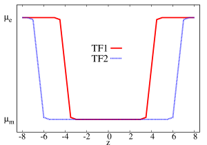
Figure 1: Sketches of the TF obtained from Eq. (30) with $z_{0}=4$ (TF1) and $z_{0}=6.5$ (TF2)

In the simulations presented here, we typically performed 10000 Monte Carlo steps (MC steps) to equilibrate the system and another 10000 MC steps to evaluate the statistical averages. Each MC step comprises $M_{p}=n_{p}\times N$ particle configuration updates (i.e., one trial move per bead on average), $M_{s}\sim 1000-20.000$ attempts to switch chain identities, and $M_{f}$ field updates, where we chose $M_{f}=1$ in the case of DDFT simulations, and $M_{f}\sim 100-1.000$ if field fluctuations are included. In some cases discussed below, we also used $M_{f}=1/3$, meaning that the fields are updated only in every third MC step. In each switch update, we switch one bead, such that roughly $M_{s}/N*0.4\sim 200$ chains are switched in one MC step for a typical acceptance rate of 0.4.

Figure 2 shows a typical simulation snapshot of the polymers in particle representation in a system with tuning function TF2. In the bulk region, very few chains are resolved by particles. Close to the boundaries, almost all chains are represented by particles. The polymers represented by fields are not shown in this snapshot.

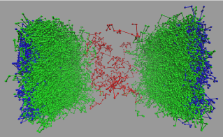
Figure 2: Simulation snapshot for polymers resolved by particles obtained with the tuning function TF2 with $\mu_{e}=0$ and $\mu_{m}=-8$. Chains in the bulk region are colored red, chains close to the impenetrable boundaries are colored blue, chains in the interfacial region between particle and field domain are colored red.

III.1 Validation of the hybrid model

We will first demonstrate that the chains can be successfully partitioned into p-chains and f-chains, and that their densities are controlled by the TF. Fig. 3 compares the density distributions in the $z$ direction as obtained from hybrid simulations of the confined system (Fig. 3) with the corresponding profiles in a bulk system of size $L_{x}\cdot L_{y}\cdot L_{z}$ without confining walls (Fig. 3). In the bulk system, a homogeneous TF generates homogeneous densities, and a large value of TF results in a large quantity of p-chains and a small quantity of f-chains. Fig. 3 demonstrates that an inhomogeneous TF that switches between $\mu_{e}=-1.5$ and $\mu_{m}=-6.5$ produces inhomogeneous densities of p-chains and f-chains, such that the p-domain with $\Delta\mu=\mu_{e}$ is mostly occupied by p-chains, and the f-domain with $\Delta\mu=\mu_{m}$ mostly by f-chains. In confined slit geometry, sharp interfaces appear near the hard walls. By choosing the TF suitably, one can enforce that polymers near the walls are represented by particles, while in the middle of the system (bulk region), most of the chains are represented by fields (Fig. 3). For the tuning function TF2, only a fraction of roughly 1/5 of all chains are p-chains (in the case of TF1, it is about 1/2). Fig. 3 also nicely demonstrates the potential applications of the hybrid method. For regions where a high resolution method is required, i.e., close to interfaces, one can use the PR method for detailed investigations, while for regions where the knowledge of density profile is sufficient, one can adopt the numerically cheaper FR method. Since the high resolution PR region occupies only a small part of the system, a hybrid simulation is more efficient than a pure particle simulation. This will be discussed more quantitatively below.

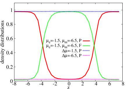
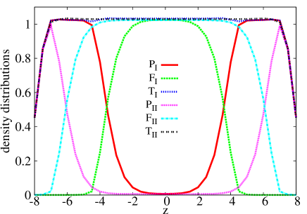
Figure 3: Density distributions obtained with the hybrid model in a bulk system (a), and in a confined slit (b). In (a) the TF is chosen as TF1 with parameters $\mu_{e}$ and $\mu_{m}$ as indicated, and in (b) the TFs are chosen as TF1 (I) and TF2 (II) with $\mu_{e}=0$ and $\mu_{m}=-8$. Here “P” refers to the density of p-chains, “F” to the density of f-chains, and “T” to the total density.

The collective properties of p-chains and f-chains, representing the physical properties of the whole system, are determined by the system parameters only (i.e., the excluded volume parameter, the size of the box, and the total number of grid points) and ideally, they should be independent of the concrete forms of the TF. However, we have already discussed in Sec. II.1 that in reality, the PR and FR representations are not fully equivalent for two reasons: First, because of the mean-field approximation that has entered the derivation of the hybrid model, and second, because of the finite grid size. The grid size affects PR and FR simulations in different ways especially close to interfaces and surfaces, where the density profiles vary strongly on the scale of single grid cells. Since the hybrid model should reproduce the properties of the particle model, the TF should be chosen such that such interfacial regions are treated at the PR level.

To test this, we focus on the density distributions and configurations of polymers close to the surfaces of the slit. Due to the impenetrability condition, the polymers are depleted near the wall. Fig. 4 compares the total density distributions obtained from the pure particle model (denoted MCP), the hybrid model (denoted PF), and the pure field model, which in our case corresponds to a standard self-consistent mean field theory (SCMF). As stated above, the pure particle model represents the reference model, whose properties should be reproduced by the other models. From Fig.4, it can be seen that the density profiles in the pure field model are steeper close to the boundaries than in the particle model, and the contact density is too low. Note that the chain resolution and the space resolution are the same for MCP and SCMF. The Edwards length $\xi_{E}$, which measures the range of fluctuation is an important quantity in field-based simulations. Usually, the lattice spacing should be chosen smaller than $\xi_{E}$. In the current work, $\xi_{E}$ is evaluated in units of $R_{\mathrm{g}}$ as $\xi_{E}\sim 0.22R_{g}$ Fredrickson , and it is a bit smaller than the lattice spacing $0.5R_{\mathrm{g}}$ but still on the same order. We checked by varying the spacing size in the SCMF theory that the density curve is almost independent of the lattice spacing. Further it can be seen from Fig.4 that the width of the depletion region near the boundary is about $R_{\mathrm{g}}$, two times larger than the lattice spacing, therefore the density difference here is not a defect of finite lattice spacing. This means that the pure field model cannot properly capture the properties of the system close to the boundary. In contrast, the total density curve obtained from the hybrid model is almost identical to that obtained from the pure particle model. In the middle of the system, which is the bulk region, all three density curves almost match. From another perspective, this means that field-based simulations can be improved by treating selected regions in space at the particle level within our hybrid scheme.

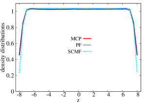
Figure 4: Total density distribution in the confined system for the pure particle model (MCP), the pure field theory (SCMF), and the hybrid model (PF) with tuning function TF2 (with $\mu_{e}=0$ and $\mu_{m}=-8.0$).

Next we inspect the polymer configurations, especially focussing on the mean-squared radius of gyration (MSRG) of chains. This quantity is easily accessible for p-chains, and it cannot be calculated for f-chains, therefore we only consider p-chains here. We cut the simulation box along the $z$ direction into $n_{z}$ slices centered at $z_{i}$ for the $i$-th slice, and the MSRGs at $z_{i}$ are defined as the corresponding averages of all the p-chains with their centers in this slice. We note that there are other quantities that can be extracted from both p-chains and f-chains, such as the chain-shape function MC_field .

Figure 5 shows the MSRG profiles of p-chains along the $z$-direction in the pure particle model and the hybrid model with TF1 and TF2. Only the profiles of the $z$-component of the MSRG ($\langle R_{gz}^{2}\rangle$) are plotted – the $x$- and $y$-components of the MSRG ($\langle R_{gx,y}^{2}\rangle$) are constant throughout and assume the value $0.33$ which is expected theoretically for Gaussian chains. The $z$-component reaches the same value in the middle of the slab (bulk region), but close to the boundaries, the polymers are a bit compressed. This can be seen both in the pure particle model and the hybrid model. The curves almost match close to the wall – in the p-domain of the hybrid model – and in the middle of the slab – in the f-domain. In the intermediate region connecting p- and f-domains, the MSRG of the p-chains in the hybrid model deviates from the MSRG measured in the particle model: It is slightly reduced at the p-side of the p/f domain boundary, and strongly enhanced at the f-side. This discrepancy can be explained by the fact that the partitioning of chains into p- and f-chains depends on their conformation in the p/f boundary region. On the f-side, p-chains that stretch into the p-domain turn into f-chains with smaller probability than p-chains that withdraw from the p-domain. Hence the remaining p-chains are on average elongated in the $z$-direction. On the p-side, the situation is the other way round: Chains that stretch into the f-domain turn into f-chains with higher probability, and the remaining p-chains are slightly compressed on average. The effect can be reduced by adopting a smoother TF, e.g., by reducing $\mu_{e}-\mu_{m}$, see the curves Ib and IIb in Fig.5, or by reducing $w$ (data not shown), but it never fully disappears. Hence it is important to realize that the p-chains in the p/f-boundary regions (within 2.5 $R_{g}$ of the boundary defined by the TF) are not representative of all chains in the system and should not be used to determine conformational properties of chains. This is a feature of the model, not an artefact.

More seriously, the total density also exhibits a very small dip in the p/f-boundary regionHybrid_PF . Deviations of the total density are also observed in other hybrid methods, and an additional potential is sometimes introduced in order to remove these artefacts CandQ ; PinningPotential . This is also an option in our model. In the present application to confined homopolymer slabs, the effect is so small that an adjustment was not necessary.

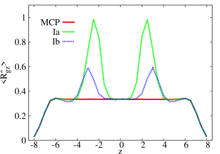
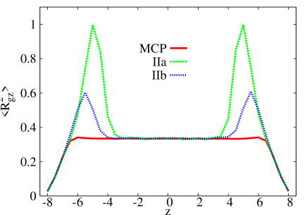
Figure 5: Profiles of the $z$-component of the MSRG of p-chains in the pure particle model (MCP) and the hybrid model with tuning function TF1 (I) and TF2 (II). Here “a” corresponds to $\mu_{e}=0$ and $\mu_{m}=-8$, while “b” refers to $\mu_{e}=-3$ and $\mu_{m}=-7.0$. Within a distance $\sim 2.5$ of the p/f-boundaries (at $z_{0}=\pm 6.5$), the conformations of p-chains in the hybrid model are not representative of the conformations of all chains.

III.2 Numerical efficiency of the hybrid model

Increasing computational efficiency is always the primary motivation for introducing multiscale schemes, and we would like to show in the following that the present hybrid method is more efficient than pure particle simulations. The computational costs of a simulation based on a particle model scales with the number of particles, while in a field description, it scales with the number $M$ of grid points that are used to discretize space (or with $M\ln M$ if Fourier methods are used). Therefore, the hybrid model is most efficient in dense systems, where the number of segments (beads) per grid cell is large. At fixed number of grid points, one can choose a TF such that the total number of p-chains is small, and this makes the simulation efficient.

In order to evaluate the efficiency of our hybrid scheme, we use the same methods to update the particle configurations in the pure particle simulation and the hybrid simulation, and perform the calculations on the same desktop computer (i7 CPU, 2.67 GHZ). We find that in each MC step, the computational cost for updating the chain configurations dominates the total costs, hence the choice of $M_{f}$ (i.e., whether we choose $M_{f}=1$ or $M_{f}=1/3$) and $M_{s}$ has little influence on the overall computational costs. However, the choice of $M_{s}$ does strongly affect the equilibration time for the effective energy. From Fig. 6, one can see that the hybrid calculation with TF1, where about half of the chains are p-chains, is roughly 1.4 times faster than the pure particle simulation, while one can achieve a speedup of a factor 3.5 with TF2, where about 1/5 of all chains are p-chains. Reducing $M_{f}$ by a factor of 3 has only a small influence on the computational costs.

Figure 6 shows the relaxation of the effective free energy to the equilibrium value. The relaxation is almost independent of $dt$ in the present system, hence we choose $dt=0.1$ for all cases. It can been seen that the pure particle method converges very rapidly, while the relaxation in the hybrid simulation is a bit slower, since additional time is necessary to equilibrate the partitioning between p-chains and f-chains. Although it takes more time to equilibrate the system within the hybrid method, this equilibration period is still very short (about 100 CPU seconds) compared to the much longer times (about 6000 CPU seconds) required for calculating the statistical averages. The hybrid method develops its high efficiency in this second stage, where data are accumulated. If the computational costs would strictly scale with the number of particles, we would reach a theoretical speedup of a factor of 5 in our system. This number is reduced due to the overhead costs for bookkeeping, field updates and switch moves (separating these costs is difficult), but we could still reach a speedup factor of 3.5. In systems where the fraction of particle resolved domains is smaller, the speedup will be even larger.

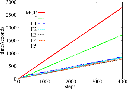
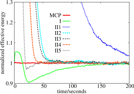
Figure 6: (a) Computational costs per MC step and (b) normalized effective energy relaxation vs. CPU time for pure particle simulations (MCP), and hybrid simulations with tuning function TF1 (I) and TF2 (II) using the parameters $\mu_{e}=0$, $\mu_{m}=-8$. The field step length is $dt=0.1$. The parameters are: $M_{f}=1/3$, $M_{s}=20000$ (I); $M_{f}=1$, $M_{s}=2500$ (II1), $M_{f}=1$, $M_{s}=7000$ (II2), $M_{f}=1/3$, $M_{s}=7000$ (II3), $M_{f}=1/3$, $M_{s}=10000$ (II4), and $M_{f}=1/3$, $M_{s}=18000$ (II5).

When judging the efficiency of a computational algorithm, another aspect that has to be considered is the complexity of the technique, and the man-hours needed to implement it. The ultimate goal is always to devise simple algorithms with high computational efficiency, although this is usually hard to achieve in practice. The new constituent in the present scheme compared to the usual particle-based MC scheme and field-based theory (e.g., self-consistent field theory) is the particle switching. Thus the hybrid scheme can be implemented by adding particle-switching algorithms that are executed after updating particle positions and fields. The switching algorithm is short and not complex, and the man-hours necessary for implementing it are less than or comparable to those required for writing a code for its pure particle-based counterpart. From a practical point of view, the main challenge is to combine particle and field simulation methods in one single package – i.e., introduce FR simulation methods in codes designed for particle simulations and vice versa. However, as explained in the introduction, there is generally a growing interest in hybrid schemes that combine particle and field methods. Within a package that can already combine particle and field-based (DDFT) simulation schemes, the implementation of our adaptive hybrid scheme should not require much effort.

III.3 Incorporation of fluctuations and outlook

In all of the above calculations, only the fluctuations of p-chains were taken into account, and those of the fields were neglected. Fluctuations sometimes play an important role in determining the properties of a dilute solution or a dense system near the critical point of a phase transition. In general one should devise methods that account for fluctuations whenever necessary. The present hybrid method does not abandon all fluctuation effects in principle, rather they are treated in different ways due to the difference of types of degrees of freedom. The configurations are sampled by the particle based method through particle moves, while the fields are sampled by the field based method through the evolution of fields. We have up to now focused on methods that neglect fluctuations in the FR part. In the following, we incorporate the fluctuations to the field by using the unbiased and biased potential sampling schemes (see subsection II.3). We choose a small size of box in the $x$ and $y$ directions with also a small number of grid points, i.e., $L_{x}=L_{y}=4$, $n_{x}=n_{y}=8$. The number of steps in updating the fields in each MC step is set $M_{f}=100$. Figure 7 shows the comparison of the density distributions obtained from the DDFT scheme, the PU and PB schemes. The parameters are chosen as $\mu_{e}=0$, $\mu_{m}=-8$. The results are independent of the step length $dt$. The curves obtained from these three different schemes are almost identical, which is expected, since the density of the polymers in the system is very high, and the fluctuation effect is expected to be small. In our applications, we find that the PB schemes is not as efficient as the PU and DDFT schemes. This may be different in more complex systems, where the bias of PB moves towards following a free energy gradient may be of advantage.

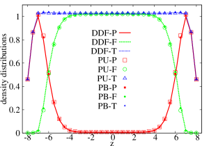
Figure 7: Densities of p-chains (P), f-chains (F) and the total density (T) obtained with the dynamic density functional scheme (DDFT), the potential unbiased algorithm (PU), and the potential biased algorithm (PB). The tuning function is chosen as TF2 with $\mu_{e}=0$ and $\mu_{m}=-8.0$. The noise amplitudes in the PU and PB schemes are chosen such that the acceptance probability is about 0.3. The densities obtained with these three schemes almost match each other.

Even if we use advanced Monte Carlo techniques such as the PB scheme to sample the field fluctuations, they do not represent the true dynamics of the system. In order to study rheological and dynamical properties, the hybrid scheme should be complemented with a consistent dynamical model. In particular, mass (particle number) and momentum should be locally conserved. Particle models with “realistic” dynamics satisfy this requirement. For example, overdamped Brownian particle simulations conserve the mass, while dissipative particle dynamics conserves both mass and momentum. On the side of the field model, the Maurits-Fraaije density_dynamics density dynamics conserves mass, at least approximately, and such DDFT models can be extended such that momentum is conserved as well zhang_11 . Difficulties in a true hybrid dynamics model arise from the requirement of mass and momentum conservation during the process of resolution switching. Several works have tried to address these notoriously difficult issues in hybrid models, see, e.g., Refs. particle_FH ; MD_FHM ; MD_SDPD ; MD_MCD . It is conceivable that particle-based Brownian simulations, combined with field-based density dynamics and a particle-field switching process which is compatible with the continuity equation for the mass, could capture the dynamics of the system at the same level as pure particle-based Brownian simulations. The construction of such a model is currently under way.

IV Summary and remarks

In the present paper, a hybrid particle-continuum simulation scheme with adaptive resolution for soft matter systems was derived based on a field-theoretical approach. In such a hybrid resolution method, polymer chains can switch their representations on the fly according to a pre-determined tuning function TF. A proper form of TF can ensure that polymer chains are described by particles in small selected regions in order to directly observe the configuration dependent properties, and by density profiles in the remaining large bulk regions, where configuration details are not interesting. Therefore, the hybrid scheme is computationally more efficient than the pure particle method, while keeping the physical accuracy in the particle regions. The hybrid approach is particularly attractive for simulations of dense systems where particle simulations become expensive compared to field-based simulations.

In the present formulation of the hybrid model, the high-resolution domains have to be determined beforehand. They may follow polymer-solid interfaces, e.g., in applications to polymer nanocomposites, but they do not explicitly depend on the polymer configuration. Hence our scheme is adaptive, but not self-adaptive. Constructing a self-adaptive scheme is another major challenge for the future. Physically, self-adaptive means that the TF should be determined by the system itself. So far, the shape of the TF is essentially a tanh function with pre-defined amplitude, offset, interface position and step width. None of these parameters is determined by the system itself. However, the optimal TF depends on the intrinsic properties of the hybrid system. For example, due to the asymmetric property of the p-chains and f-chains, a non-zero reference value of $\Delta\mu$ where the fraction of p- and f-chains is equal can be calculated which can then be used as offset. Concerning the step width and the locations of the p/f interfaces, one possible and practical way is to directly relate them to the local density and/or the local density gradient. The tuning function could be chosen such that it has large values in interfacial regions (where the total density curve has a large slope) and low values in the bulk (where the slope is zero). This should give the desired result that p-chains aggregate in the interface while f-chains are dominant in the bulk. Such hybrid models could then be called self-adaptive resolution models in the sense that the chains described by different resolution models can switch and redistribute according to the local density. We will explore this option in future work.

The present hybrid model is constructed such that it targets polymer solutions. However, the basic idea of the hybrid model can be applied to other systems. The approach is especially suitable for very large systems with large bulk regions and small interface regions or small regions that need detailed investigation. One example is a polymer brush system, in which a small number of brush polymers are attached to a plate, while a large number of polymers remain in the bulk. For such a system, the hybrid model is recommended. The brush polymers can be treated by higher resolution method, i.e., the PR method, to catch the more detailed properties (for example, the lengths of chains), while the large bulk region can be treated by lower resolution method, i.e., the FR method, to save time.

The studies of a homopolymer solution using the hybrid scheme show good agreement with those by the reference pure particle method, and the hybrid scheme has demonstrated its higher computational efficiency. However, so far, it can only be used to study static properties. In future work, we will extend this hybrid scheme such that it can also be used to study dynamical properties and flow behavior in complex fluids.

ACKNOWLEDGMENTS

We thank Stefan Dolezel, Sebastian Meinhardt, Liangshun Zhang, and Jiajia Zhou for helpful discussions and suggestions. This project is supported by the German Science Foundation (DFG) within project C1 in SFB TRR 146. Simulations were run on the computer cluster Mogon at the University of Mainz.

References

- (1) Polymer Surfaces and Interfaces: Characterization, Modification and Application, M. Stamm Edt., Springer, Berlin, 2008.
- (2) G. Kickelbick, Progr. Pol. Science 28, 83 (2003).
- (3) F. Mammeri, E. Le Bourhis, L. Rozes, C. Sanches, J. Materials. Chem. 15, 3787 (2005).
- (4) T. Kulla, S. Bhadra, D.H. Yao, N.H. Kim, S. Bose, J.H. Lee, Progr. Polym. Sci. 35, 1350 (2010).
- (5) P. van Rijn, H. Park, K.Ö Nazli, N.C. Mougin, A. Böker, Langmuir 29, 276 (2013).
- (6) D. Guo, G. Xie, J. Luo, J. Phys. D: Appl. Phys. 47, 013001 (2014).
- (7) F. Mathias, A. Fokina, K. Landfester, W. Tremel, F. Schmid, K. Char, R. Zentel, Macrom. Rapid Comm. 36, 959 (2015).
- (8) A. Warshel, M. Levitt, J. Mol. Biology 103, 227 (1976).
- (9) M.J. Field, P.A. Bash, M. Karplus, J. Comp. Chem. 11, 700 (1990).
- (10) J. Baschnagel, K. Binder, P. Doruker, A.A. Gusev, O. Hahn, K. Kremer, W.L. Mattice, F. Müller-Plathe, M. Murat, W. Paul, S. Santos, U.W. Suter, V. Tries Adv. Polym. Sci. 152, 41 (2000).
- (11) W. E, B. Engquist, X. Li, W. Ren, E. Vanden-Eijnden, Comm. Comput. Phys. 2, 367 (2007).
- (12) S.A. Baeurle, J. Math. Chem. 46, 363 (2009).
- (13) C. Peter, K. Kremer, Soft Matter 5, 4357 (2009).
- (14) D. Lockerby, A. Patronix, M.K. Borg, J.M. Reese, J. Comp. Phys. 284, 261 (2015).
- (15) M. Praprotnik, L. Delle Site, K. Kremer, Annu. Rev. Phys. Chem. 59, 545 (2008).
- (16) M. Praprotnik, L. Delle Site, K. Kremer, J. Chem. Phys. 123, 224106 (2005).
- (17) B. Ensing, S.O. Nielsen, P.B. Moore, M.L. Klein, M. Parrinello, J. Chem. Theory Comput. 3, 1100 (2007).
- (18) A. Heyden, D.G. Truhlar, J. Chem. Theory Comput. 4, 217 (2008).
- (19) M. Praprotnik, L. Delle Site, K. Kremer, Phys. Rev. E. 73, 066701 (2006).
- (20) A.B. Poma, L. Delle Site. Phys. Rev. Lett. 104, 250201 (2010).
- (21) A.B. Poma, L. Delle Site, Phys. Chem. Chem. Phys. 13, 10510 (2011).
- (22) C.S. Peskin, Acta Numerica 11, 479 (2002)
- (23) P.J. Atzberger, P.R. Kramer, C.S. Peskin, J. Comput. Phys. 224, 1255 (2007).
- (24) S.W. Sides, B.J. Kim, E.J. Kramer, G.H. Fredrickson, Phys. Rev. Lett. 96, 250601 (2006).
- (25) G.J.A. Sevink, M. Charlaganov, J.G.E.M. Fraaije, Soft Matter 9, 2816 (2013).
- (26) W. E and Z. Huang, Phys. Rev. Lett. 87, 135501 (2001).
- (27) V. Ganesan, V. Pryamitsyn, J. Chem. Phys. 118, 4345 (2003).
- (28) B. Narayanan, V.A. Pryamitsyn, V. Ganesan, Macromolecules 37, 10180 (2004).
- (29) M. Müller, G.D. Smith, J. Polym. Sci.: Part B: Polym. Phys. 43, 934 (2005).
- (30) K. Ch Daoulas, M. Müller, J. Chem. Phys. 125 184904 (2006).
- (31) G. Milano, T. Kawakatsu, J. Chem. Phys. 130, 214106 (2009).
- (32) G. Milano, T. Kawakatsu, J. Chem. Phys. 133, 214102 (2010).
- (33) G. Milano, T. Kawakatsu, A. de Nicola, Phys. Biol. 10, 045007 (2013).
- (34) R. Delgado-Buscalioni, P.V. Coveney, Phys. Rev. E 67, 046704 (2003).
- (35) G. De Fabritiis, R. Delgado-Buscalioni, P.V. Coveney, Phys. Rev. Lett. 97, 134501 (2006).
- (36) R. Delgado-Buscalioni, G. De Fabritiis, Phys. Rev. E 76, 036709 (2007).
- (37) R. Delgado-Buscalioni, K. Kremer, M. Praprotnik, J. Chem. Phys. 128, 114110 (2009).
- (38) L.D. Landau, E.M. Lifshitz, Statistical Physics Part 2 Theory of Condensed State Second edition (Pergamon Press, 1980).
- (39) S. Qi, H. Behringer, F. Schmid, New J. Phys. 15, 125009 (2013).
- (40) S.F. Edwards, Proc. Phys. Soc. 85, 613 (1965).
- (41) G.H. Fredrickson, H. Orland, J. Chem. Phys. 140, 084902 (2014).
- (42) P.G. de Gennes, Rep. Prog. Phys. 32, 187 (1969).
- (43) S.F. Edwards, Proc. Phys. Soc. 88, 265 (1966).
- (44) M. Muthukumar, S.F. Edwards, J. Chem. Phys. 76, 2760 (1982).
- (45) K. Freed, Renormalization Group Theory of Macromolecules (New York: Wiley, 1987).
- (46) M. Laradji, H. Guo, M.J. Zuckermann, Phys. Rev. E. 49, 3199 (1994).
- (47) M.P. Stoykovich, M. Müller, S.O. Kim, H.H. Solak, E.W. Edwards, J.J. de Pablo, P.F. Nealey, Science 308, 1442 (2005).
- (48) F.A. Detcheverry, D.Q. Pike, P.F. Nealey, M. Müller, J.J. de Pablo, Phys. Rev. Lett. 102, 197801 (2009).
- (49) P. Gemünden, H. Behringer, J. Chem. Phys. 138, 024904 (2013).
- (50) S. Qi, L. I. Klushin, A. M. Skvortsov, A. A. Polotsky, F. Schmid, Macromolecules, 48, 3775 (2015).
- (51) E. Helfand, J. Chem. Phys. 62, 999 (1975).
- (52) G. Besold, H. Guo, M.J. Zuckermann, J. Poly. Sci. Part B: Polym. Phys. 38, 1053 (2000).
- (53) D. Frenkel, B. Smit, Understanding Molecular Simulation: From Algorithms to Applications, (New York: Academic Press, 2002
- (54) G. H. Fredrickson, The Equilibrium Theory of Inhomogeneous Polymers (Oxford University Press, Oxford, 2006).
- (55) G.H. Fredrickson, V. Ganesan, F. Drolet, Macromolecules 35, 16 (2002).
- (56) F. Schmid, J. Phys.: Condens. Matter 10, 8105 (1998).
- (57) K.M. Hong, J. Noolandi, Macromolecules 14, 727 (1981).
- (58) A. Alexander-Katz, A.G. Moreira, S.W. Sides, G.H. Fredrickson, J. Chem. Phys. 122, 014904 (2005).
- (59) Z.-G. Wang, J. Chem. Phys. 117, 481 (2002).
- (60) A. Kudlay, S. Stepanow, J. Chem. Phys. 118, 4272 (2003).
- (61) P. Grzywacz, J. Qin, D.C. Morse, Phys. Rev. E 76, 061802 (2007).
- (62) V. Ganesan, G.H. Frederickson, Europhys. Lett. 55, 814 (2001).
- (63) K. Freed, Adv. Chem. Phys. 22, 1 (1972).
- (64) F.A. Detcheverry, H. Kang, K. Ch Daoulas, M. Müller, P.F. Nealey, J.J. de Pablo, Macromolecules 41, 4989 (2008).
- (65) M. Müller, J. Stat. Phys. 145, 967 (2011).
- (66) P.J. Rossky, J.D. Doll, H.L. Friedman, J. Chem. Phys. 69, 4628 (1978).
- (67) D.A. Kofke, E.D. Glandt, Mol. Phys. 64, 1105 (1988).
- (68) K. Ch. Daoulas, D. N. Theodorou, V. A. Harmandaris, N. Ch. Karayiannis, V. G. Mavrantzas, Macromolecules 38, 7134 (2005).
- (69) S. Fritsch, S. Poblete, C. Junghans, G. Ciccotti, L. Delle Site, K. Kremer, Phys. Rev. Lett. 108, 170602 (2012).
- (70) N.M. Maurits, J.G.E.M. Fraaije, J. Chem. Phys. 108, 5879 (1997).
- (71) L. Zhang, A. Sevink, F. Schmid, Macromolecules 44, 9434 (2011).
- (72) N.D. Petsev, L.G. Leal, M.S. Shell, J. Chem. Phys. 142, 044101 (2015).
- (73) U. Alekseeva, R. G. Winkler, G. Sutmann, J. Comput. Phys., 314, 14 (2016).