Using model distances to investigate
the simplifying assumption, model selection
and truncation levels for vine copulas

Abstract

Vine copulas are a useful statistical tool to describe the dependence structure between several random variables, especially when the number of variables is very large. When modeling data with vine copulas, one often is confronted with a set of candidate models out of which the best one is supposed to be selected. For example, this may arise in the context of non-simplified vine copulas, truncations of vines and other simplifications regarding pair-copula families or the vine structure. With the help of distance measures we develop a parametric bootstrap based testing procedure to decide between copulas from nested model classes. In addition we use distance measures to select among different candidate models. All commonly used distance measures, e.g. the Kullback-Leibler distance, suffer from the curse of dimensionality due to high-dimensional integrals. As a remedy for this problem, Killiches, Kraus and Czado (2017b) propose several modifications of the Kullback-Leibler distance. We apply these distance measures to the above mentioned model selection problems and substantiate their usefulness.

Keywords: Vine copulas, Kullback-Leibler distance, model selection, simplifying assumption, truncated vines.

1 Introduction

In a world of growing data sets and rising computational power the need of adequately modeling multivariate random quantities is self-evident. Since the seminal paper of Sklar, (1959) the modeling of a multivariate distribution function can be divided into separately considering the marginal distributions and the underlying dependence structure, the so-called copula. One of the most popular copula classes, especially for high-dimensional data, are vine copulas (Aas et al.,, 2009). Constructing a multivariate copula in terms of bivariate building blocks, this pair-copula construction has the advantage of being highly flexible while still yielding interpretable models. Vines have been extensively used for high-dimensional copula modeling. Brechmann and Czado, (2013) analyzed the interdependencies of the stocks contained in the Euro Stoxx 50 for risk management purposes, while Stöber and Czado, (2014) considered the detection of regime switches in high-dimensional financial data. Müller and Czado, (2017) used Gaussian directed acyclic graphs to facilitate the estimation of vine copulas in very high dimensions. Moreover, in the context of big data, gene expression data and growing market portfolios, the interest in high-dimensional data modeling cannot be expected to decline.

In model selection, the distance between statistical models plays a big role. Usually the difference between two statistical models is measured in terms of the Kullback-Leibler (KL) distance (Kullback and Leibler,, 1951). Model selection procedures based on the KL distance for copulas are developed for example in Chen and Fan, (2005), Chen and Fan, (2006) and Diks et al., (2010). In the context of vine copulas, Joe, (2014) used the KL distance to calculate the sample size necessary to discriminate between two densities. Investigating the simplifying assumption Hobæk Haff et al., (2010) used the KL distance to find the simplified vine closest to a given non-simplified vine and Stöber et al., (2013) assessed the strength of non-simplifiedness of the trivariate Farlie-Gumbel-Morgenstern (FGM) copula for different dependence parameters.

Nevertheless, the main issue of the Kullback-Leibler distance is that, as soon as it cannot be computed analytically, a numerical evaluation of the appearing integral is needed, which is hardly tractable once the model dimension exceeds three or four. In order to tackle this problem, several modifications of the Kullback-Leibler distance have been proposed in Killiches et al., 2017b . They yield model distances which are close in performance to the classical KL distance, however with much faster computation times, facilitating their use in very high dimensions. While the examples presented in that paper are mainly plausibility checks underlining the viability of the proposed distance measures, the aim of this paper is to demonstrate their usefulness in three practical problems. First, we investigate a major question arising when working with vines: Is the simplifying assumption justified for a given data set or do we need to account for non-simplifiedness? The importance of this topic can be seen from many recent publications such as Hobæk Haff et al., (2010), Stöber and Czado, (2012), Acar et al., (2012), Spanhel and Kurz, (2015) or Killiches et al., 2017a . Then we show how to select the best model out of a list of candidate models with the help of a model distance based measure. Finally, we also use the new distance measures to answer the question how to determine the optimal truncation level of a fitted vine copula, a task already recently discussed by Brechmann et al., (2012) and Brechmann and Joe, (2015). Truncation methods have the aim of enabling high-dimensional vine copula modeling by severely reducing the number of used parameters without changing the fit of the resulting model too much.

The remainder of the paper is structured as follows. In Section 2 we shortly introduce vine copulas and the distance measures proposed in Killiches et al., 2017b . Further, we provide a hypothesis test facilitating model selection. In Section 3 we show how this test can be used to decide between simplified and non-simplified vines. Section 4 describes how the proposed distance measures can be applied to assess the best model fit out of a set of candidate models. As a final application the determination of the optimal truncation level of a vine copula is discussed in Section 5. Finally, Section 6 concludes.

2 Theoretical concepts

2.1 Vine copulas

Copulas are $d$-dimensional distribution functions on $[0,1]^{d}$ with uniformly distributed margins. The usefulness of the concept of copulas has become clear with the publication of Sklar, (1959), where the famous Sklar’s Theorem is proven. It provides a link between an arbitrary joint distribution and its marginal distributions and dependence structure. This result has been very important for applications since it allows the marginals and the dependence structure to be modeled separately. An introduction to copulas can be found in Nelsen, (2006); Joe, (1997) also contains a thorough overview over copulas.

Although there is a multitude of multivariate copula families (e.g. Gaussian, t, Gumbel, Clayton and Joe copulas), these models exhibit little flexibility in higher dimensions. Introducing vine copulas, Bedford and Cooke, (2002) proposed a way of constructing copula densities by combining bivariate building blocks. Aas et al., (2009) applied the concept of vines, also referred to as pair-copula constructions (PCCs), and used them for statistical inference.

In the following we consider a $d$-dimensional random vector $\mathbf{U}=(U_{1},\ldots,U_{d})^{\top}$ with uniform marginals $U_{j}$, $j=1,\ldots,d$, following a copula $C$ with corresponding copula density $c$. For $j\in\left\{1,\ldots,d\right\}$ and $D\subseteq\left\{1,\ldots,d\right\}\setminus\left\{j\right\}$ we denote by $C_{j|D}$ the conditional distribution function of $U_{j}$ given $\mathbf{U}_{D}=(U_{i})_{{i\in D}}$. For $j,k\in\left\{1,\ldots,d\right\}$ and $D\subseteq\left\{1,\ldots,d\right\}\setminus\left\{j,k\right\}$ the copula density of the distribution associated with the conditioned variables $U_{j}$ and $U_{k}$ given the conditioning variables $\mathbf{U}_{D}$ is denoted by $c_{j,k;D}$.

The structure of a $d$-dimensional vine copula is organized by a sequence of trees $\mathcal{V}=(T_{1},\ldots,T_{d-1})$ satisfying

1. $T_{1}=(V_{1},E_{1})$ is a tree with nodes $V_{1}=\left\{1,\ldots,d\right\}$ and edges $E_{1}$;

2. For $m=2,\ldots,d-1$, the tree $T_{m}$ consists of nodes $V_{m}=E_{m-1}$ and edges $E_{m}$;

3. Whenever two nodes of $T_{m}$ are connected by an edge, the corresponding edges of $T_{m-1}$ share a node ($m=2,\ldots,d-1$).

In a vine copula model each edge of the $d-1$ trees corresponds to a bivariate pair-copula. Let $\bigcup_{m=1}^{d-1}\left\{c_{j_{e},k_{e};D_{e}}\mid e\in E_{m}\right\}$ be the set of pair-copulas associated with the edges in $\mathcal{V}$, where – following the notation of Czado, (2010) – $j_{e}$ and $k_{e}$ denote the indices of the conditioned variables $U_{j_{e}}$ and $U_{k_{e}}$ and $D_{e}$ represents the conditioning set corresponding to edge $e$. The vine density can be written as

$$c(u_{1},\ldots,u_{d})=\prod_{m=1}^{d-1}\prod_{e\in E_{m}}c_{j_{e},k_{e};D_{e}}\left(C_{j_{e}|D_{e}}(u_{j_{e}}|\mathbf{u}_{D_{e}}),C_{k_{e}|D_{e}}(u_{k_{e}}|\mathbf{u}_{D_{e}});\mathbf{u}_{D_{e}}\right).$$ (2.1)

As an example we show a possible tree structure of a five-dimensional vine copula in Figure 1. All appearing edges are identified with a pair-copula in the vine decomposition. For example, the third tree contains the specifications of $c_{1,3;4,5}$ and $c_{2,3;4,5}$.

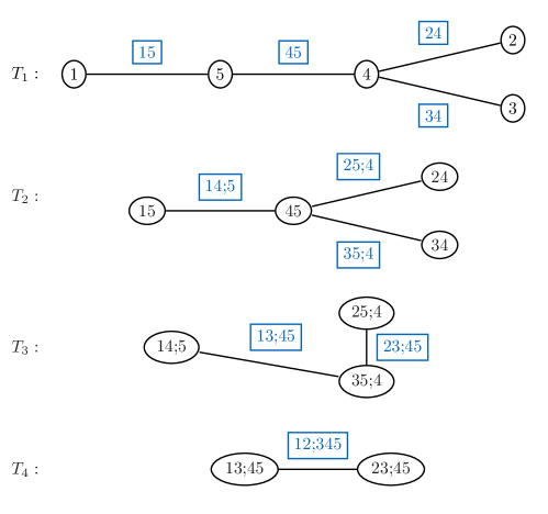
Figure 1: Tree sequence of an exemplary five-dimensional vine copula.

Vine copulas with arbitrary tree structure are often referred to as regular vines or in short R-vines. Special cases of vine copula structures are so-called D-vines and C-vines. For a D-vine each node in tree $T_{1}$ has a degree of at most $2$ such that the trees are simply connected paths. In a C-vine for each tree $T_{m}$ there exists a root node with degree $d-m$, i.e. it is a neighbor of all other nodes. Each tree then has a star-like structure.

Note that in general the pair-copula $c_{j_{e},k_{e};D_{e}}$ depends on the conditioning value $\mathbf{u}_{D_{e}}$. In order to reduce model complexity and to enable statistical inference even in high dimensions, one often makes the so-called simplifying assumption that the influence of $\mathbf{u}_{D_{e}}$ can be neglected and $c_{j_{e},k_{e};D_{e}}$ is equal for all possible values of $\mathbf{u}_{D_{e}}$.

Stöber et al., (2013) investigated which multivariate copulas could be represented as simplified vines: Similar to the relationship between correlation matrices and partial correlations (Bedford and Cooke,, 2002), every Gaussian copula can be written as a simplified Gaussian vine, i.e. a vine copula with only bivariate Gaussian pair-copulas, where any (valid) vine structure can be used and the parameters are the corresponding partial correlations. Vice versa, every Gaussian vine represents a Gaussian copula. Further, t copulas can also be decomposed into simplified vines with arbitrary (valid) vine structure. The pair-copulas are then bivariate t copulas, the association parameters are the corresponding partial correlations and the degrees of freedom in tree $T_{m}$ are $\nu+(m-1)$, where $\nu$ is the degrees of freedom parameter of the t copula. However, a regular vine copula with only bivariate t copulas, called a t vine, does not necessarily represent a t copula.

The so-called Dißmann algorithm (cf. Dißmann et al.,, 2013) is a treewise sequential algorithm that fits a simplified vine copula model to a given data set, where pairs with high dependence are modeled in lower trees in order to keep the induced estimation bias low. It is also implemented in the R package VineCopula (Schepsmeier et al.,, 2017) as RVineStructureSelect.

2.2 Model distances for vine copulas

In this section we shortly review the definitions of the most important distance measures discussed in Killiches et al., 2017b . For detailed information about the concepts consult this paper and references therein. Starting point is the so-called Kullback-Leibler distance (see Kullback and Leibler,, 1951) between two $d$-dimensional copula densities $c^{f}$, $c^{g}\colon[0,1]^{d}\to[0,\infty)$, defined as

$$\operatorname{KL}(c^{f},c^{g})=\int_{\mathbf{u}\in[0,1]^{d}}\ln\left(\frac{c^{f}(\mathbf{u})}{c^{g}(\mathbf{u})}\right)c^{f}(\mathbf{u})\mathop{}\!\mathrm{d}\mathbf{u}.$$ (2.2)

Note that due to the lack of symmetry the KL distance is not a distance in the classical sense and therefore is also referred to as Kullback-Leibler divergence. If $c^{f}$ and $c^{g}$ are the corresponding copula densities of two $d$-dimensional densities $f$ and $g$, it can be easily shown that the KL distance between $c^{f}$ and $c^{g}$ is equal to the one between $f$ and $g$ if their marginal distributions coincide. It is common practice to use the Inference Functions for Margins (IFM) method: First the univariate margins are estimated and observation are transform to the copula scale; afterwards the copula is estimated based on the transformed data (cf. Joe,, 1997, Section 10.1). Therefore, it can be justified that in the remainder of the paper we restrict ourselves to data on the copula scale.

Since in the vast majority of cases the KL distance cannot be calculated analytically, the main problem of using the KL distance in practice is the computational intractability for dimensions larger than 4. There, numerical integration suffers from the curse of dimensionality and thus becomes exceptionally inefficient. As a remedy for this issue, Proposition 2 from Killiches et al., 2017b expresses the KL between multivariate densities in terms of the sum of expected KL distances between univariate conditional densities:

$$\operatorname{KL}\big{(}c^{f},c^{g}\big{)}=\sum_{j=1}^{d}\mathbb{E}_{c^{f}_{(j+1):d}}\Big{[}\operatorname{KL}\Big{(}c^{f}_{j|(j+1):d}\left(\,\cdot\,|\mathbf{U}_{(j+1):d}\right),c^{g}_{j|(j+1):d}\left(\,\cdot\,|\mathbf{U}_{(j+1):d}\right)\Big{)}\Big{]},$$ (2.3)

where for $j<d$ we use the abbreviation $(j+1)\!:\!d=\left\{j+1,j+2,\ldots,d\right\}$ with ${(d+1)\!:\!d}:=\emptyset$ and $\mathbf{U}_{(j+1):d}\sim c^{f}_{(j+1):d}$. It would be a valid approach to approximate the expectations in Equation (missing) 2.3 by Monte Carlo integration, i.e. the average over evaluations of the integrand on a grid of points simulated according to $c^{f}_{(j+1):d}$. Since this would also be computationally challenging in higher dimensions and additionally has the disadvantage of being random, Killiches et al., 2017b propose to approximate the expectations through evaluations on a grid consisting of only warped diagonals in the respective unit (hyper)cube. The resulting diagonal Kullback-Leibler (dKL) distance between two $d$-dimensional R-vine models $\mathcal{R}^{f}$ and $\mathcal{R}^{g}$ is hence defined by

$$\operatorname{dKL}\left(\mathcal{R}^{f},\mathcal{R}^{g}\right)=\sum_{j=1}^{d-1}\frac{1}{|\mathcal{D}_{j}|}\sum_{\mathbf{u}\in\mathcal{D}_{j}}\operatorname{KL}\left(c^{f}_{j|(j+1):d}(\cdot|\mathbf{u}),c^{g}_{j|(j+1):d}(\cdot|\mathbf{u})\right),$$

where the set of warped discrete diagonals $\mathcal{D}_{j}\in[0,1]^{d-j}$ is given by

$$\mathcal{D}_{j}=T_{j}\left(\left\{\left\{\mathbf{r}+\mu\mathbf{v}(\mathbf{r})\mid\mu\in\mathcal{I}_{\varepsilon,n}\right\}\,\middle|\,\mathbf{r}\in\left\{0,1\right\}^{d-j}\right\}\right).$$

Here, $\mathbf{r}\in\left\{0,1\right\}^{d-j}$ are the corner points in the unit hypercube $\left[0,1\right]^{d-j}$, $\mathbf{v}\colon\left\{0,1\right\}^{d-j}\rightarrow\left\{-1,1\right\}^{d-j}$, $\mathbf{v}(\mathbf{r})=\boldsymbol{1}-2\mathbf{r}$ denotes the direction vector from $\mathbf{r}$ to its opposite corner point and $\mathcal{I}_{\varepsilon,n}$ is the equidistantly discretized interval $[\varepsilon,1-\varepsilon]$ of length $n$. Hence $\left\{\mathbf{r}+\mu\mathbf{v}(\mathbf{r})\mid\mu\in\mathcal{I}_{\varepsilon,n}\right\}$ represents a discretization of the diagonal from $\mathbf{r}$ to its opposite corner point $\mathbf{r}+\mathbf{v}(\mathbf{r})$. Finally, these discretized diagonals are transformed using is the inverse Rosenblatt transformation $T_{j}$ with respect to $c^{f}_{(j+1):d}$ (Rosenblatt,, 1952). Recall that the Rosenblatt transformation $\mathbf{u}$ of a vector $\mathbf{w}\in[0,1]^{d}$ with respect to a distribution function $C$ is defined by $u_{d}=w_{d}$, $u_{d-1}=C_{d-1|d}^{-1}(w_{d-1}|u_{d})$, $\ldots$ , $u_{1}=C_{1|2:d}^{-1}(w_{1}|u_{2},\ldots,u_{d})$. Often it is used to transform a uniform sample on $[0,1]^{d}$ to a sample from $C$. The concept is used to transform the unit hypercube’s diagonal points to points with high density values of $c^{f}_{(j+1):d}$ Hence, the KL distance between $c^{f}$ and $c^{g}$ is approximated by evaluating the KL distances between the univariate conditional densities $c^{f}_{j|(j+1):d}$ and $c^{g}_{j|(j+1):d}$ conditioned on values lying on warped diagonals $\mathcal{D}_{j}$, $j=1,\ldots,d-1$. Diagonals have the advantage that all components take values on the whole range from 0 to 1 covering especially the tails, where the substantial differences between copula models occur most often. With the above modifications the intractability of the KL for multivariate densities is overcome since only KL distances between univariate densities have to be evaluated. It was shown in Proposition 1 of Killiches et al., 2017b that these univariate conditional densities $c^{f}_{j|(j+1):d}$ and $c^{g}_{j|(j+1):d}$ can be easily derived for the vine copula model. Moreover, in Remark 1 they prove that for $\varepsilon\to 0$ and $n\to\infty$ the dKL converges to a sum of scaled line integrals. Further, they found heuristically that even for $n=10$ and $\varepsilon=0.025$ the dKL was a good and fast substitute for the KL distance.

Nevertheless, since the number of diagonals grows exponentially in the dimension, Killiches et al., 2017b found that for really high dimensions (e.g. $d>20$) the computation of the dKL was rather slow. However, they illustrated in several examples that the restriction of the evaluations to a single principle diagonal yields exceptionally fast calculations and still results in a viable distance measure with qualitative outcomes close to the KL distance. For $j<d$, out of the set $\mathbb{D}_{j}$ of the $2^{(d-j)-1}$ possible $(d-j)$-dimensional diagonals, the principal diagonal $\mathcal{D}_{j}^{*}$ is the one with the largest weight, measured by an integral over the diagonal with respect to the density $c^{f}_{(j+1):d}$, i.e.

$$\mathcal{D}_{j}^{*}=\operatorname{arg\,max}\limits_{\mathcal{D}\in\mathbb{D}_{j}}\int_{\mathbf{x}\in D}c^{f}_{(j+1):d}(\mathbf{x})\mathop{}\!\mathrm{d}\mathbf{x}.$$

Hence, the single diagonal Kullback-Leibler distance between $\mathcal{R}^{f}$ and $\mathcal{R}^{g}$ is given by

$$\operatorname{sdKL}(\mathcal{R}^{f},\mathcal{R}^{g})=\sum_{j=1}^{d-1}\frac{1}{|\mathcal{D}^{*}_{j}|}\sum_{\mathbf{u}\in\mathcal{D}^{*}_{j}}\operatorname{KL}\left(c^{f}_{j|(j+1):d}(\cdot|\mathbf{u}),c^{g}_{j|(j+1):d}(\cdot|\mathbf{u})\right).$$

In practice it has shown to be advisable to use the dKL for dimensions $d<10$ and the sdKL for higher-dimensional applications. For a more detailed discussion on implementation and performance of these distance measures we refer to Killiches et al., 2017b .

Without further reference it is not possible to decide whether a given distance measure value is large or small. Therefore in the following we develop a statistical test to decide whether a distance value is significantly different from zero.

2.3 Hypothesis test for model selection

In this section we provide a procedure based on parametric bootstrapping (see Efron and Tibshirani,, 1994) for choosing between a parsimonious and a more complex model. Assume we have two nested classes of $d$-dimensional parametric copula models $\mathbb{C}^{f}\subseteq\mathbb{C}^{g}$ and a copula data set $\mathbf{u}_{i}^{0}\in[0,1]^{d}$, $i=1,\ldots,N$, with true underlying distribution $\mathcal{R}^{g}\in\mathbb{C}^{g}$. We want to investigate whether a model from $\mathbb{C}^{f}$ suffices to describe the data. In other words, we want to test the null hypothesis $H_{0}\colon\mathcal{R}^{g}\in\mathbb{C}^{f}$, which means that there exists $\mathcal{R}^{f}\in\mathbb{C}^{f}$ such that $\mathcal{R}^{f}=\mathcal{R}^{g}$. Due to the identity of indiscernibles (i.e. $\operatorname{KL}(\mathcal{R}^{f},\mathcal{R}^{g})=0$ if and only if $\mathcal{R}^{f}=\mathcal{R}^{g}$) of the Kullback-Leibler distance this is equivalent to $\operatorname{KL}(\mathcal{R}^{f},\mathcal{R}^{g})=0$. Hence, for testing $H_{0}$ we can examine whether the KL distance between $\mathcal{R}^{f}$ and $\mathcal{R}^{g}$ is significantly different from zero. In practice, $\mathcal{R}^{f}$ and $\mathcal{R}^{g}$ are unknown and have to be estimated from the data $\mathbf{u}_{i}^{0}\in[0,1]^{d}$. Consider the KL distance $d_{0}=\operatorname{KL}(\hat{\mathcal{R}}_{0}^{f},\hat{\mathcal{R}}_{0}^{g})$ between the two fitted models $\hat{\mathcal{R}}_{0}^{f}$ and $\hat{\mathcal{R}}_{0}^{g}$ as the test statistic. Since the distribution of $d_{0}$ cannot be derived analytically we use the following parametric bootstrapping scheme to retrieve it:

For $j=1,\ldots,M$, generate a sample $\mathbf{u}^{j}_{i}\in[0,1]^{d}$, $i=1,\ldots,N$, from $\hat{\mathcal{R}}_{0}^{f}$. Fit copulas $\hat{\mathcal{R}}^{f}_{j}\in\mathbb{C}^{f}$ and $\hat{\mathcal{R}}^{g}_{j}\in\mathbb{C}^{g}$ to the generated sample. Calculate the distance between $\hat{\mathcal{R}}^{f}_{j}$ and $\hat{\mathcal{R}}^{g}_{j}$:

$$d_{j}=\operatorname{KL}(\hat{\mathcal{R}}^{f}_{j},\hat{\mathcal{R}}^{g}_{j}).$$

Now reorder the set $\left\{d_{j}\mid j=1,\ldots,M\right\}$ such that $d_{1}<d_{2}<\ldots<d_{M}$. For a significance level $\alpha\in(0,1)$, we can determine an empirical confidence interval $I_{1-\alpha}^{M}\subseteq\left[0,\infty\right)$ with confidence level $1-\alpha$ by

$$I_{1-\alpha}^{M}=[0,d_{\lceil M(1-\alpha)\rceil}],$$

where $\lceil\cdot\rceil$ denotes the ceiling function. Finally, we can reject $H_{0}$ if $d_{0}\notin I_{1-\alpha}^{M}$. Figure 2 illustrates the above procedure in a flow chart. At the bottom the resulting distances are plotted on the positive real line. In this exemplary case, $d_{0}$ (circled cross) lies outside the range of the empirical $100(1-\alpha)\%$ confidence interval and therefore $H_{0}$ can be rejected at the $100\alpha\%$ level, i.e. there is a significant difference between $\hat{\mathcal{R}}_{0}^{f}$ and $\hat{\mathcal{R}}_{0}^{g}$.

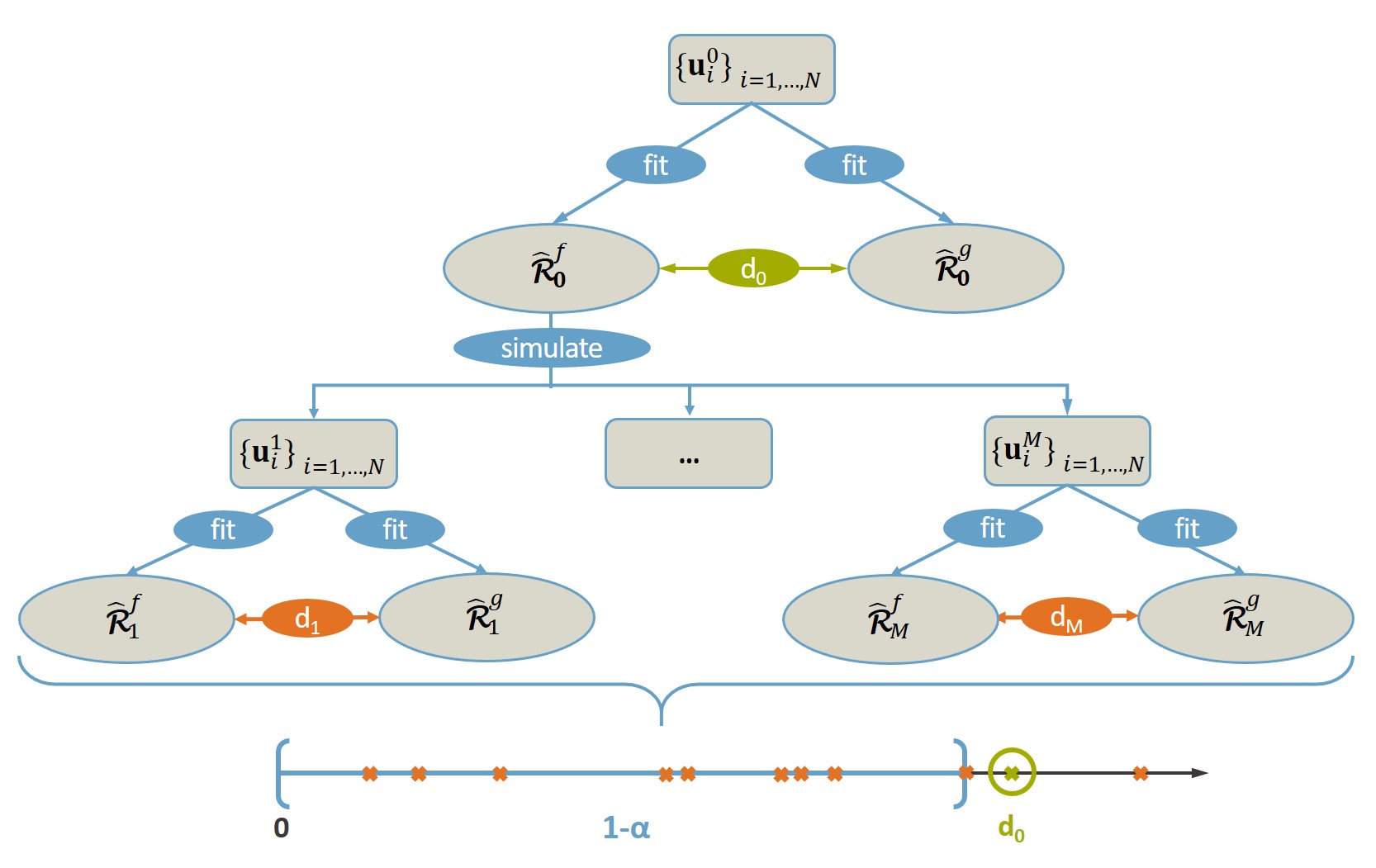
Figure 2: Scheme of the testing procedure based on parametric bootstrapping.

Since in higher dimensions the KL distance cannot be calculated in a reasonable amount of time, we use the distance measures dKL (for $d<10$) and sdKL (for $d\geq 10$), introduced in Section 2.2, as substitutes for the KL distance. The above bootstrapping scheme works similarly using the substitutes.

Of course, it is not obvious per se how to choose the number of bootstrap samples $M$. On the one hand we want to choose $M$ as small as possible (due to computational time); on the other hand we want the estimate of $d_{\lceil M(1-\alpha)\rceil}$ to be as precise as possible in order to avoid false decisions with respect to the null hypothesis (the upper bound $d_{\lceil M(1-\alpha)\rceil}$ of the confidence interval $I_{1-\alpha}^{M}$ is random with variance decreasing in $M$). Therefore, we choose $M$ so large that $d_{0}$ lies outside the $100(1-\beta)\%$ confidence interval of $d_{\lceil M(1-\alpha)\rceil}$ such that we can decide whether $d_{0}$ is significantly larger (smaller) than $d_{\lceil M(1-\alpha)\rceil}$. This confidence interval can be obtained from an estimate of the distribution of the $\lceil M(1-\alpha)\rceil$th order statistic (see for example Casella and Berger,, 2002, page 232). In all applications of this test contained in this paper we found that for $\alpha=5\%$ and $\beta=1\%$ a bootstrap sample size of $M=100$ was enough.

Validity of the parametric bootstrap for the hypothesis test

In order to establish the validity the parametric bootstrap for the above hypothesis test we will argue that under the null hypothesis $H_{0}$ the bootstrapped distances $d_{j}$, $j=1,\ldots,M$, are i.i.d. with a common distribution that is close to $F_{d_{0}}$, i.e. the distribution of $d_{0}$, for large sample size $N$: If we have a consistent estimator for $\mathcal{R}^{f}$, we know that under $H_{0}$ the estimate $\hat{\mathcal{R}}^{f}$ is close to $\mathcal{R}^{f}$ for large $N$. Since the bootstrap samples $\mathbf{u}_{i}^{j}$, $i=1,\ldots,N$, $j=1,\ldots,M$ are generated from $\hat{\mathcal{R}}^{f}$, they can be assumed to be approximate samples from $\mathcal{R}^{f}$. Since $\hat{\mathcal{R}}^{f}_{j}$ and $\hat{\mathcal{R}}^{g}_{j}$ are estimated based on the $j$th bootstrap sample $\mathbf{u}_{i}^{j}$, $i=1,\ldots,N$, the KL between $\hat{\mathcal{R}}^{f}_{j}$ and $\hat{\mathcal{R}}^{g}_{j}$, i.e. $d_{j}$, has the same distribution as the KL between $\hat{\mathcal{R}}^{f}$ and $\hat{\mathcal{R}}^{g}$, i.e. $d_{0}$, for large $N$. Therefore, we can construct empirical confidence intervals for $d_{0}$ based on the bootstrapped distances $d_{j}$, $j=1,\ldots,M$.

Of course this argumentation is not a strict proof but rather makes the proposed approach plausible. An example for a mathematical justification of the parametric bootstrap in the copula context can be found in Genest and Rémillard, (2008). In Section 3.1 we will see in a simulation study that our proposed test holds its level under the null hypothesis (for different sample sizes) when investigating the power of the test in a simplified/non-simplified vine copula framework.

3 Testing simplified versus non-simplified vine copulas

As already mentioned in the introduction, the validity of the simplifying assumption is a frequently discussed topic in the recent literature. For the case the simplifying assumption is not satisfied, Vatter and Nagler, (2016) developed a method to fit a non-simplified vine to given data such that the parameters of the pair-copulas with non-empty conditioning sets are dependent on the conditioning variable(s). This functional relationship is modeled with a generalized additive model. The fitting algorithm is implemented in the R package gamCopula (Vatter,, 2016) as the function gamVineStructureSelect. The selection of the vine structure is identical to the one of RVineStructureSelect.

In this section we will present how distance measures can be used to decide whether a (more complicated) non-simplified model is needed or the simplified model suffices. This can be done with the help of the test introduced in Section 2.3 (using the dKL). Here we take $\mathbb{C}^{f}$ and $\mathbb{C}^{g}$ to be the class of simplified and non-simplified vine copula models, respectively. Since every simplified vine can be represented as a non-simplified vine with constant parameters, $\mathbb{C}^{f}$ and $\mathbb{C}^{g}$ are nested, i.e. $\mathbb{C}^{f}\subseteq\mathbb{C}^{g}$. Now, the null hypothesis $H_{0}$ to be tested at significance level $\alpha$ is that the true underlying model is in $\mathbb{C}^{f}$, i.e. the model is simplified.

After investigating the power of the test (Section 3.1) we apply it to a hydro-geochemical and a financial data set in Section 3.2.

3.1 Power of the test

In a simulation study we investigate the performance of our test. For this purpose we consider a three-dimensional non-simplified vine consisting of the pair-copulas $c_{1,2}$, $c_{2,3}$ and $c_{1,3;2}$, where all pairs are bivariate Clayton copulas. The Kendall’s $\tau$ values of the copulas $c_{1,2}$ and $c_{2,3}$ are $\tau_{1,2}=0.7$ and $\tau_{2,3}=0.5$, respectively. The third $\tau$ value depends linearly on $u_{2}$: $\tau_{1,3;2}(u_{2})=a+(b-a)u_{2}$ with constants $a,b\in[-1,1]$. For $a=b$ the function is constant such that the vine is simplified. By construction $\tau_{1,3;2}$ can become negative for some combinations of $a$, $b$ and $u_{2}$; in such cases we use the 90 degree rotated version of the Clayton copula since the Clayton copula does not allow for negative dependence.

By fixing $a=0.3$ and letting $b$ range between $-1$ and $1$ in $0.1$ steps we obtain 21 scenarios. For each of the scenarios we generate a sample of size $N\in\left\{200,500,1000\right\}$ from the corresponding non-simplified vine copula and fit both a simplified and a non-simplified model to the generated data. Since we are only interested in the parameters and their variability we fix both the vine structure and the pair-copula families to the true ones. We test the null hypothesis that the two underlying models are equal. In order to assess the power of the test, we perform this procedure $P=250$ times (at significance level $\alpha=5\%$) and check how many times the null hypothesis is rejected. As sample size we take the same $N$ used to generate the original data. In each test we perform $M=100$ bootstrap replications. In Figure 3 the proportions of rejections of the null hypothesis within the $P=250$ performed tests are shown depending on $b$. The different sample sizes are indicated by the three different curves: $N=200$ (dotted curve), $N=500$ (dashed curve) and $N=1000$ (solid curve).

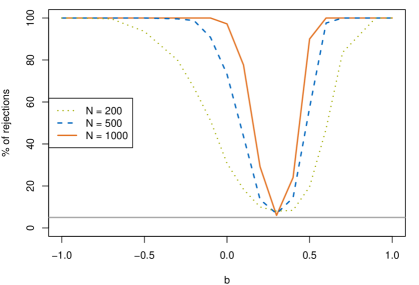
Figure 3: Percentage of rejections of $H_{0}$ (at level $\alpha=5\%$) depending on $b$ with constants $a=0.3$, $M=100$ and $P=250$ for $N=200$ (dotted curve), $N=500$ (dashed curve) and $N=1000$ (solid curve). The horizontal solid gray line indicates the 5% level.

We see that the observed power of the test is in general very high. Considering the dashed curve, corresponding to a sample size of $N=500$, one can see the following: If the distance $\left|b-a\right|$ is large, $\tau_{1,3;2}$ is far from being constant. Hence, we expect the non-simplified vine and the simplified vine to be very different and therefore the power of the test to be large. We see that for $b\leq-0.1$ and $b\geq 0.6$ the power of the test is above $80\%$ and for $b\leq-0.2$ and $b\geq 0.7$ it is even (close to) $100\%$. For values of $b$ closer to $a$ the power decreases. For example, for $b=0.1$ the Kendall’s $\tau$ value $\tau_{1,3;2}$ only ranges between 0.1 and 0.3 implying that the non-simplified vine does not differ too much from a simplified vine. Therefore, we cannot expect the test to always detect this difference. Nevertheless, even in this case the power of the test is estimated to be almost $44\%$. From a practical point of view, this result is in fact desirable since models estimated based on real data will always exhibit at least slight non-simplifiedness due to randomness even when the simplifying assumption is actually satisfied. Further, for $b=0.3$ the function $\tau_{1,3;2}(u_{2})$ is actually constant with respect to $u_{2}$ so that $\mathcal{R}^{*}$ is a simplified vine. Thus, $H_{0}$ is true and we hope to be close to the significance level $\alpha=5\%$. With $6.4\%$ of rejections, we see that this is the case here.

Looking at the dotted and the solid curve we find that the higher the sample size is, the higher is the power of the test, which is what one also would have expected. In the case of $N=1000$, we have a power of over $80\%$ for $b\in[-1,0]\cup[0.5,1]$ and even $100\%$ rejections for $b\in[-1,-0.1]\cup[0.6,1]$. For $b=0.3$ the test holds its level with $5.2\%$ of rejections. Yet even for a sample size of as little as $N=200$, the power of the test is above $80\%$ for values of $b$ between $-1$ and $-0.3$ and $0.5$ and $1$. A power of $100\%$ is reached for $b\leq-0.8$ and $b\geq 0.9$. For $b=0.3$ the test rejects the null hypothesis in $7.2\%$ of the cases.

We can conclude that our test is a valid $\alpha$-level method in finite samples to decide if a non-simplified model is necessary.

3.2 Real data examples

Three-dimensional subset of the uranium data set

To show an application of our test we use a subset of the classical seven-dimensional hydro-geochemical data set (Cook and Johnson,, 1986), which has amongst others been investigated by Acar et al., (2012) and Killiches et al., 2017a with respect to the simplifying assumption. The data set consists of $N=655$ observations of log concentrations of different chemicals in water samples from a river near Grand Junction, Colorado. We will focus on the three chemicals cobalt ($U_{1}$), titanium ($U_{2}$) and scandium ($U_{3}$) and fit both a simplified and a non-simplified vine copula to the data.

The fitted simplified vine $\hat{\mathcal{R}}_{0}^{f}$ is specified in the following way: $c_{1,2}$ is a t copula with $\tau_{1,2}=0.53$ and $\nu_{1,2}=8.03$, $c_{2,3}$ is a t copula with $\tau_{2,3}=0.43$ and $\nu_{2,3}=5.93$ and $c_{1,3;2}$ is a t copula with $\tau_{1,3;2}=0.08$ and $\nu_{1,3;2}=5.65$. For the non-simplified vine $\hat{\mathcal{R}}_{0}^{g}$, the pair-copulas $c_{1,2}$ and $c_{2,3}$ are the same as for the simplified vine, $c_{1,3;2}$ is also still a t copula but now has $\nu_{1,3;2}=6.69$ degrees of freedom and its association parameter depends on $u_{2}$ as displayed as the solid line in Figure 4. For values of $u_{2}$ below 0.8 (roughly) we have small positive Kendall’s $\tau$ values, whereas for the remaining values we observe small to medium negative association. For comparison, the (constant) Kendall’s $\tau$ of the estimated simplified vine is plotted as a dashed line. Further, the pointwise bootstrapped 95% confidence bounds under $H_{0}$ are indicated by the gray area.

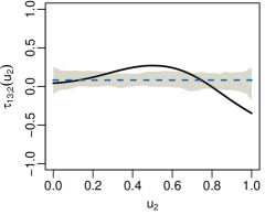
Figure 4: Estimated functional relationship between $\tau_{1,3;2}$ and $u_{2}$ (for the non-simplified model $\hat{\mathcal{R}}_{0}^{g}$). The dashed line represents the constant $\tau_{1,3;2}$ of the simplified model $\hat{\mathcal{R}}_{0}^{f}$ and the gray area indicates the pointwise bootstrapped 95% confidence bounds under $H_{0}$.

The fact that the estimated Kendall’s $\tau$ function exceeds these bounds for more than half of the $u_{2}$ values suggests that the simplified and non-simplified vines are significantly different from each other. We now use our testing procedure to formally test this.

The distance between the two vines is $\operatorname{dKL}_{0}=0.058$. In order to test the null hypothesis we generate $M=100$ samples of size $N=655$ from $\hat{\mathcal{R}}_{0}^{f}$. Then, for each sample we estimate a non-simplified vine $\hat{\mathcal{R}}^{g}_{j}$ and a simplified vine $\hat{\mathcal{R}}^{f}_{j}$ and calculate the distance between them. Since with one exception all resulting simulated distances are considerably smaller than $\operatorname{dKL}_{0}$, we can reject $H_{0}$ at the 5% level (with a p-value of 0.01). Hence, we conclude that here it is necessary to model the dependence structure between the three variables using a non-simplified vine. Acar et al., (2012) and Killiches et al., 2017a also come to the conclusion that a simplified vine would not be sufficient in this example.

Four-dimensional subset of the EuroStoxx 50 data set

We examine a 52-dimensional EuroStoxx50 data set containing 985 observations of returns of the EuroStoxx50 index, five national indices and the stocks of the 46 companies that were in the EuroStoxx50 for the whole observation period (May 22, 2006 to April 29, 2010). This data set will be studied more thoroughly in Section 5.3. Since fitting non-simplified vine copulas in high dimensions would be too computationally demanding we consider only a four-dimensional subset containing the following national indices: the German DAX ($U_{1}$), the Italian MIB ($U_{2}$), the Dutch AEX ($U_{3}$) and the Spain IBEX ($U_{4}$) (see also Example 1 of Killiches et al., 2017b , where this data set was already investigated). In practice it is very common to model financial returns using multivariate t copulas (see e.g. Demarta and McNeil,, 2005). From Stöber et al., (2013) we know that any multivariate t copula can be represented as a vine satisfying the simplifying assumption. With our test we can check whether this necessary condition is indeed fulfilled for this particular financial return data set.

We proceed as in the previous section and fit a simplified model $\hat{\mathcal{R}}_{0}^{f}$ as well as a non-simplified model $\hat{\mathcal{R}}_{0}^{g}$ to the data. The estimated structures of both models are C-vines with root nodes DAX, MIB, AEX and IBEX. Again, the pair-copulas in the first tree coincide for both models being fitted as bivariate t copulas with $\tau_{1,2}=0.70$ and $\nu_{1,2}=4.96$, $\tau_{1,3}=0.72$ and $\nu_{1,3}=6.23$, and $\tau_{1,4}=0.69$ and $\nu_{1,2}=6.80$. In the second tree of the simplified model the pair-copulas are also estimated to be t copulas with $\tau_{2,3;1}=0.23$ and $\nu_{1,2}=6.34$, and $\tau_{2,4;1}=0.24$ and $\nu_{1,2}=10.77$. The corresponding non-simplified counterparts fitted by the gamVineStructureSelect algorithm are also t copulas, whose strength of dependence varies only very little and stays within the confidence bounds of the simplified vine (see Figure 5, left and middle panel). The estimated degrees of freedom are also quite close to the simplified ones ($\nu_{2,3;1}=6.47$ and $\nu_{2,4;1}=11.56$), such that regarding the second tree we would presume that the distance between both models is negligible. Considering the copula $c_{3,4;1,2}$ in the third tree, the simplified fit is a Frank copula with $\tau_{3,4;1,2}=0.11$, while the non-simplified fit is a Gaussian copula whose $\tau$ values only depend on $u_{1}$ (i.e. the value of the DAX). In the right panel of Figure 5 we see the estimated relationship, which is a bit more varying than the others but still mostly stays in between the confidence bounds. The broader confidence bounds can be explained by the increased parameter uncertainty for higher order trees of vine copulas arising due to the sequential fitting procedure.

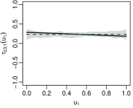
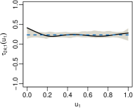
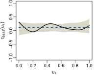
Figure 5: Estimated functional relationship of $\tau_{2,3;1}$ (left), $\tau_{2,4;1}$ (middle) and $\tau_{3,4;1,2}$ (right) in terms of $u_{1}$ from $\hat{\mathcal{R}}_{0}^{g}$. The dashed lines represent the constant $\tau$ values of the simplified model $\hat{\mathcal{R}}_{0}^{f}$ and the gray areas indicate the pointwise bootstrapped 95% confidence bounds under $H_{0}$.

The question is now, whether the estimated non-simplified vine is significantly different from the simplified one, or in other words: Is it necessary to use a non-simplified vine copula model for this data set or does a simplified one suffice?

In order to answer this question we make use of our test using parametric bootstrapping and produce $M=100$ simulated distances under the null hypothesis that both underlying models are equivalent. In this case the original distance between $\hat{\mathcal{R}}_{0}^{f}$ and $\hat{\mathcal{R}}_{0}^{g}$ is close to the lower quartile and therefore the null hypothesis clearly cannot be rejected. So we can conclude that for this four-dimensional financial return data set a simplified vine suffices to reasonably capture the dependence pattern.

In a next step we test with the procedure from Section 2.3 ($\alpha=5\%$, $M=100$) whether there is a significant difference between the above fitted simplified vine and a t copula. With a p-value of $0.10$ we cannot reject the null hypothesis that the two underlying models coincide such that it would be justifiable to assume a t copula to be the underlying dependence structure of this financial return dataset.

Although we only presented applications in dimensions 3 and 4, in general the procedure can be used in arbitrary dimensions. The computationally limiting factor is the fitting routine of the non-simplified vine copula model, which can easily be applied up to 15 dimensions in a reasonable amount of time (for the methods implemented in Vatter,, 2016).

4 Model selection

A typical application of model distance measures is model selection. Given a certain data set one often has to choose between several models with different complexity and features. Distance measures are a convenient tool that can help with the decision for the “best” or “most suitable” model out of a set of candidate models.

4.1 KL based model selection

The Kullback-Leibler distance is of particular interest for model selection because of the following relationship: For given copula data $\mathbf{u}_{i}\in[0,1]^{d}$, $i=1,\ldots,N$, from a $d$-dimensional copula model $c\colon[0,1]^{d}\to[0,\infty)$ we have

$$\operatorname{KL}(c,c^{\perp})\approx\sum_{i=1}^{N}\log\left(\frac{c(\mathbf{u}_{i})}{c^{\perp}(\mathbf{u}_{i})}\right)=\sum_{i=1}^{N}\log\left(c(\mathbf{u}_{i})\right)=\log\ell(c),$$

where $c^{\perp}$ denotes the density of the $d$-dimensional independence copula and $\log\ell(c)$ is the log-likelihood of the model $c$. This means that the log-likelihood of a model can be approximated by calculating its Kullback-Leibler distance from the corresponding independence model (also known as mutual information in the bivariate case; see e.g. Cover and Thomas,, 2012). The log-likelihood itself as well as the information criteria AIC and BIC (Akaike,, 1998; Schwarz,, 1978), which are based on the log-likelihood but penalize the use of too many parameters, can be used to assess how well a certain model fits the data. The higher (lower) the log-likelihood (AIC/BIC) is, the better the model fit. Thus, a high Kullback-Leibler distance from the independence copula also corresponds to a good model fit. Note that this approximation only holds if data in fact was generated from $c$. Since in applications the true underlying distribution $c$ is unknown, we can use the KL distance between a fitted copula and the independence copula as a proxy for the quality of the fit. Therefore, having fitted different models to a data set it is advisable to choose the one with the largest KL distance. Since dKL and sdKL are modifications of the original KL distance, it is natural to use them as substitutes for the model selection procedure.

In the following subsections we provide two examples, where dKL and sdKL based measures are applied for model selection. For this purpose we perform the following procedure 100 times: We fix a vine copula model and generate a sample of size $N=3000$ from it. Then, we fit different models and calculate the distance to the independence model with respect to dKL and sdKL, respectively. The results are compared to AIC and BIC.

4.2 Five-dimensional mixed vine

As a first example we consider a five-dimensional vine copula with the vine tree structure given in Figure 1 from Section 2.1 and the following pair-copulas:

• Tree 1: $c_{1,5}$ is a Gumbel copula with $\tau_{1,5}=0.6$, $c_{2,4}$ is a BB1 copula with $\tau_{2,4}=0.83$, $c_{3,4}$ is a BB7 copula with $\tau_{3,4}=0.74$ and $c_{4,5}$ is a Tawn copula with $\tau_{4,5}=0.72$;

• Tree 2: $c_{1,4;5}$ is a Clayton copula with $\tau_{1,4;5}=0.5$, $c_{2,5;4}$ is a Joe copula with $\tau_{2,5;4}=0.45$ and $c_{3,5;4}$ is a BB6 copula with $\tau_{3,5;4}=0.48$;

• Tree 3: $c_{1,3;4,5}$ is a t copula with $\tau_{1,3;4,5}=-0.19$ and $\nu_{1,3;4,5}=3$ degrees of freedom and $c_{2,3;4,5}$ is a Frank copula with $\tau_{2,3;4,5}=-0.31$;

• Tree 4: $c_{1,2;3,4,5}$ is a Gaussian copula with $\tau_{1,2;3,4,5}=-0.13$.

As described above, we perform the following steps 100 times: Generate a sample of size $N=3000$ from the specified vine copula and fit four different models to the data sample (a Gaussian copula, a C-vine, a D-vine and an R-vine). Table 1 displays the number of parameters, the dKL to the five-dimensional independence copula and the AIC and BIC values of the four fitted models, all averaged over the 100 replications. The corresponding estimated standard errors are given in brackets.

	# par	$\operatorname{dKL}(\,\cdot\,,c^{\perp})$	AIC	BIC
Gaussian copula	$\mathbf{10.00}\,(0.00)$	$6.24\,(0.09)$	$-23669\,(377)$	$-23609\,(377)$
C-vine	$15.57\,(0.64)$	$7.10\,(0.06)$	$-28317\,(333)$	$-28223\,(333)$
D-vine	$19.77\,(0.47)$	$7.41\,(0.08)$	$-30320\,(354)$	$-30201\,(354)$
R-vine	$15.68\,(0.78)$	$\mathbf{8.37}\,(0.06)$	$\mathbf{-33843}\,(344)$	$\mathbf{-33749}\,(345)$

Table 1: Average number of parameters, dKL to the five-dimensional independence copula, AIC and BIC of the fitted Gaussian copula, C-vine, D-vine and R-vine. Standard errors are given in brackets. Best values per column are marked in bold.

Compared to the 15 parameters of the true model, the Gaussian copula has only 10 parameters but also exhibits the poorest fit of all considered models with respect to any of the decision criteria. The C-vine (between 15 and 16 parameters on average) is ranked third by dKL, AIC and BIC. The D-vine model uses the most parameters (almost 20) but also performs better than the C-vine. With just under 16 parameters on average the R-vine copula is rated best by all three measures. We see that the ranking of the four fitted models is the same for dKL, AIC and BIC. We also checked that all 100 cases yielded this ranking. Considering the empirical ‘noise-to-signal’ ratio, i.e. the quotient of the standard errors and the absolute estimated mean, we obtain that the dKL performs better than AIC and BIC (e.g. for the R-vine we have $0.06/8.37<344/33843<345/33479$).

4.3 20-dimensional t vine

In order to show a high-dimensional example, we consider a 20-dimensional D-vine being also a t vine, i.e. a vine copula with only bivariate t copulas as pair copulas. The association parameter is chosen constant for all pair-copulas in one tree: Kendall’s $\tau$ in Tree $m$ is $0.8^{m}$, $m=1,\ldots,19$. Further, all pairs are heavy-tailed, having $\nu=3$ degrees of freedom. Due to the overall constant degrees of freedom the resulting t vine with its 380 parameters is not a t copula (cf. Section 2.1). Now we repeat the following procedure 100 times: Generate a sample of size $N=3000$ from the t vine and fit a Gaussian copula, a t copula, a t vine and an R-vine with arbitrary pair-copula families to the simulated data. Since the calculation of the dKL in $d=20$ dimensions would be rather time-consuming, we use the sdKL instead. We present the number of parameters, the sdKL to the 20-dimensional independence copula and the AIC and BIC values of the four fitted models (again averaged over the 100 replications) in Table 2. The estimated standard errors are given in brackets.

	# par	$\operatorname{sdKL}(\,\cdot\,,c^{\perp})$	AIC	BIC
Gaussian copula	$\mathbf{190.00}\,(0.00)$	$84.11\,(0.75)$	$-271610\,(2962)$	$-270468\,(2962)$
t copula	$191.00\,(0.00)$	$93.95\,(0.67)$	$-299703\,(1929)$	$-298556\,(1929)$
t vine	$380.00\,(0.00)$	$96.72\,(0.82)$	$\mathbf{-309647}\,(2112)$	$\mathbf{-307365}\,(2112)$
R-vine	$379.87\,(0.60)$	$\mathbf{96.80}\,(0.99)$	$-309337\,(2579)$	$-307056\,(2579)$

Table 2: Average number of parameters, sdKL to the 20-dimensional independence copula, AIC and BIC of the fitted Gaussian copula, t copula, t vine and R-vine. Standard errors are given in brackets. Best values per column are marked in bold.

The Gaussian copula has the least parameters (190) but also the worst sdKL, AIC and BIC values. Adding a single additional parameter already causes an enormous improvement of all three measures for the t copula. The t vine is more flexible but has considerably more parameters than the t copula (380); nevertheless all three decision criteria prefer the t vine over the t copula. Surprisingly, the t vine is even ranked a little bit higher by AIC and BIC than the R-vine, which also has roughly 380 parameters on average. This ranking might seem illogical at first because the class of R-vines is a superset of the class of t vines such that one would expect the fit of the R-vine to be at least as good as the fit of the t vine. The reason for this alleged contradiction is that the fitting procedure that is implemented in the R package VineCopula (Schepsmeier et al.,, 2017) is not optimizing globally but tree-by-tree (cf. Section 2.1). Therefore, it is possible that fitting a non-t copula in one of the lower trees might be optimal but cause poorer fits in some of the higher trees. However, the difference between the fit of the t vine and the R-vine is very small and for 83 of the 100 samples both procedures fit the same model. Therefore, we want to test whether this difference is significant at all. For this purpose, we perform a parametric bootstrapping based test as described in Section 2.3 at the level $\alpha=5\%$ with $M=100$ replications. With p-values between $0.32$ and $0.78$ we cannot even reject the null hypothesis that the two underlying models coincide in any of the remaining 17 cases, where different models were fitted. Hence we would prefer to use the simpler t vine model which is in the same model class as the true underlying model. In a similar manner we check whether the difference between the t copula and the t vine is significant. Here, however, we find out that the model can indeed be distinguished at a $5\%$ confidence level for all 100 samples (p-values range between $0$ and $0.03$). Considering the empirical noise-to-signal ratio we see that sdKL is a bit more dependent on the sample compared to dKL such that AIC, BIC and sdKL have roughly the same noise-to-signal ratio, where the values of AIC/BIC are slightly lower for the t copula, the t vine and the R-vine.

5 Determination of the optimal truncation level

As the dimension $d$ of a vine copula increases, the number of parameters $d(d-1)/2$ grows quadratically. For example, a 50-dimensional R-vine consists of 1225 (conditional) pair-copulas, each with one or more copula parameters. This on the one hand can create computational problems, while on the other hand the resulting model is difficult to interpret. Given an $d$-dimensional data set ($d$ large), it has been proposed (see Brechmann et al.,, 2012; Brechmann and Joe,, 2015) to fit a so-called $k$-truncated vine, where the pair-copulas of all trees of higher order than some truncation level $k\leq d-1$ are modeled as independence copulas. This reduces the number of pair-copulas to be estimated from $d(d-1)/2$ to $k(k-1)/2$, where $k$ is chosen as small as can be justified. The heuristic behind this approach is that the sequential fitting procedure of regular vines captures most of the dependence in the lower trees, such that the dependence in the higher trees might be negligible and therefore the approximation error caused by using an independence copula is rather small. The task of finding the optimal truncation level $k^{*}$ has already been tackled in the recent literature. Brechmann et al., (2012) use likelihood based criteria such as the AIC, BIC and Vuong test for the selection of $k^{*}$, while Brechmann and Joe, (2015) propose an approach based on fit indices that measure the distance between fitted and observed correlation matrices.

5.1 Algorithms for the determination of optimal truncation levels

Using the proposed distance measures we can directly compare several truncated vines with different truncation levels. With the bootstrapped confidence intervals described in Section 2.3 we can assess whether the distances are significant in order to find the optimal truncation level. To be precise, in the following we present two algorithms that use the sdKL for the determination of the optimal truncation level, a global one (Algorithm 1) and a sequential one (Algorithm 2).

In Algorithm 1, tRV($k$) denotes the $k$-truncated version of RV. Since a full $d$-dimensional R-vine consists of $d-1$ trees, tRV($d-1$) and RV coincide.

Algorithm 1 Global determination of the optimal truncation level

Input: $d$-dimensional copula data, significance level $\alpha$.

1:Fit full (non-truncated) regular vine $\text{RV}=\text{tRV}($d-1$)$ to the data set.

2:for $m=d-2,\ldots,0$ do

3:      Specify the truncated vine tRV($m$) by setting all pair-copulas of trees $m+1$ and higher to the independence copula.

4:      Calculate the sdKL between RV and tRV($m$) and use the parametric bootstrap to check whether the distance is significantly different from zero.

5:     if distance is significant then

6:         break the for-loop and return the optimal truncation level $k^{*}=m+1$.      

Output: Optimal truncation level $k^{*}=m+1$.

The algorithm starts with the full model RV and, going backwards, truncates the vine tree-by-tree until the distance between the $m$-truncated vine and the full model is significantly larger than 0. Hence, the truncation at level $m$ is too restrictive such that we select the level $k^{*}=m+1$, for which the distance was still insignificant. For the testing procedure we can use the test from Section 2.3 since the class of truncated vine copula models is nested in the general class of all vine copulas.

Since fitting a full vine copula model might be rather time-consuming in high dimensions with Algorithm 2 we propose another procedure of determining the truncation level, which builds the R-vine sequentially tree by tree, starting with the first tree. In each step we check whether the additionally modeled tree significantly changes the resulting model in comparison to the previous one. As long as it does, the vine is updated to one with an additionally modeled tree. Only when the addition of a new tree of order $m$ results in a model that is statistically indistinguishable from the previous one, the algorithm stops and returns the optimal truncation level $k^{*}=m-1$.

Algorithm 2 Sequential determination of the optimal truncation level

Input: $d$-dimensional copula data, significance level $\alpha$.

1:Set tRV(0) to be a truncated vine with truncation level 0, i.e. an independence copula.

2:for $m=1,\ldots,d-1$ do

3:      Specify the truncated vine tRV($m$) by taking the truncated vine from the previous step tRV($m-1$) and estimating the pair-copulas from tree $m$.

4:      Calculate the sdKL between tRV($m-1$) and tRV($m$) and use the parametric bootstrap to check whether the distance is significantly different from zero.

5:     if distance is not significant then

6:         break the for-loop and return the optimal truncation level $k^{*}=m-1$      

Output: Optimal truncation level $k^{*}=m-1$

The heuristic behind Algorithm 2 is that since the vine is estimated sequentially maximizing the sum of absolute (conditional) Kendall’s $\tau$ values in each tree (for details see Dißmann et al.,, 2013), we can expect the distance between two subsequent truncated vines to be decreasing. Therefore, if the distance between tRV($k^{*}$) and tRV($k^{*}+1$) is not significant, the distances between tRV($m$) and tRV($m+1$) for $m>k^{*}$ should be not significant either.

Comparing Algorithm 1 and Algorithm 2, we note that in general they do not find the same truncation level. For example, consider the case where for some $m$ the distances between tRV($m$) and tRV($m+1$), tRV($m+1$) and tRV($m+2$), until tRV($d-2$) and tRV($d-1$) are not significant, while the distance between tRV($m$) and tRV($d-1$) is. Then, Algorithm 2 would return an optimal truncation level of $m$, whereas we would obtain a higher truncation level by Algorithm 1. So in general we see that Algorithm 2 finds more parsimonious models than Algorithm 1.

In the following we examine how well the proposed algorithms for finding optimal truncation levels for R-vines work in several simulated scenarios as well as real data examples. We compare our results to the existing methodology of Brechmann et al., (2012), who use a Vuong test (with and without AIC/BIC correction) to check whether there is a significant difference between a certain $k$-truncated vine and the corresponding vine with truncation level $k-1$, for $k=1,\ldots,d-1$. Starting with the lowest truncation levels, once the difference is not significant for some $m$, the algorithm stops and returns the optimal truncation level $k^{*}=m-1$.

5.2 Simulation study

20-dimensional t copula truncated at level 10

In the first simulated example, we consider a scenario where the data comes from a 20-dimensional t copula truncated at level 10. For this, we set the degrees of freedom to 3 and produce a random correlation matrix sampled from the uniform distribution on the space of correlation matrices (as described in Joe,, 2006). In this example, the resulting correlations range between $-1$ and $1$ with a higher concentration on correlations with small absolute values. After sampling the correlation matrix, we express the corresponding t copula as a D-vine (cf. Section 2.1) and truncate it at level 10, i.e. the pair-copulas of trees 11 to 19 are set to the independence copula. From this truncated D-vine we generate a sample of size $N=2000$ and use the R function RVineStructureSelect from the package VineCopula to fit a vine copula to the sample with the Dißmann algorithm (see Section 2.1). The question is now if our algorithms can detect the true truncation level underlying the generated data. For this we visualize the steps of the two algorithms. Concerning Algorithm 1, in the left panel of Figure 6 we plot the sdKL-distances between the truncated vines and the full (non-truncated) vine against the 19 truncation levels together with the bootstrapped 95% confidence bounds ($d_{95}$ from Section 2.3) under the null hypothesis that the truncated vine coincides with the full model (dashed line).

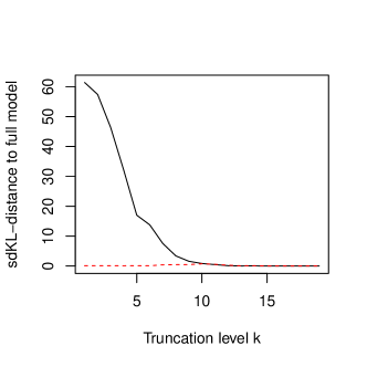
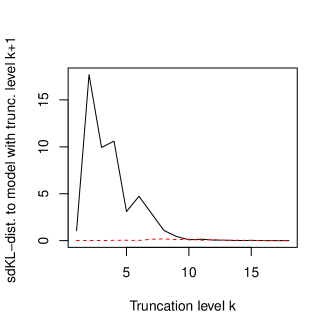
Figure 6: Visualization of the algorithms for data generated from a 20-dimensional t copula truncated at level 10.
Left (Algorithm 1): sdKL-distance to full model with dashed bootstrapped 95% confidence bounds.
Right (Algorithm 2): sdKL-distance to model with truncation level $k+1$ with dashed bootstrapped 95% confidence bounds.

Naturally, the curve corresponding to Algorithm 1 is decreasing with an extremely large distance between the one-truncated vine and the full model and a vanishingly small distance between the 18-truncated vine and the full model, which only differ in the specification of one pair-copula. In order to determine the smallest truncation level whose distance to the full model is insignificantly large, the algorithm compares these distances to the bootstrapped 95% confidence bounds. In this example we see that the smallest truncation level for which the sdKL-distance to the full model drops below the confidence bound is 10, such that the algorithm is able to detect the true truncation level. In order to check, whether this was not just a coincidence we repeated this procedure 100 times and found that the optimal truncation level found by the algorithm averages to 10.5 with a standard deviation of 0.81.

The right panel of Figure 6 displays the results for Algorithm 2. For each truncation level $k$, the sdKL-distance between the vine truncated at level $k$ and the vine truncated at level $k+1$ is plotted, again together with bootstrapped 95% confidence bounds under the null hypothesis that this distance is 0, i.e. the true model is the one with truncation level $k$. We observe that the largest sdKL-distance is given between the vine copulas truncated at levels 2 and 3, 3 and 4, and 4 and 5, respectively. This is in line with the results from Algorithm 1 (left panel of Figure 6), where we observe the steepest decrease in sdKL to the full model from truncation level 2 to 5. In this example Algorithm 2 would also detect the true truncation level 10. In the 100 simulated repetitions of this scenario, the average optimal truncation level was 10.2 with a standard deviation of 0.41.

In each of the 100 repetitions, we also used the Vuong test based algorithms without/with AIC/with BIC correction from Brechmann et al., (2012) to compare our results. They yielded average truncation levels of 14.6, 12.6 and 10.8 (without/with AIC/with BIC correction), depending on the correction method. So all three methods overestimate the truncation level, in particular the first two.

Thus we have seen that in a scenario where the data is generated from a truncated vine both our proposed algorithms manage to detect the truncation level very well. Next, we are interested in the results of the algorithms when the true underlying copula is not truncated.

20-dimensional t copula (non-truncated)

In this example we generate data from the same 20-dimensional t copula as before, this time without truncating it. The results of the algorithms are displayed in Figure 7.

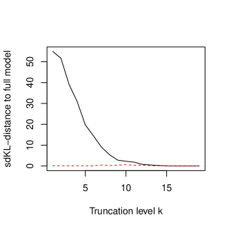
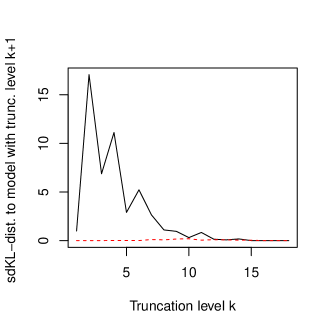
Figure 7: Visualization of the algorithms for data generated from a 20-dimensional t copula (non-truncated).
Left (Algorithm 1): sdKL-distance to full model with dashed bootstrapped 95% confidence bounds.
Right (Algorithm 2): sdKL-distance to model with truncation level $k+1$ with dashed bootstrapped 95% confidence bounds.

At first sight the plots look quite similar to those of Figure 6. Due to the sequential fitting algorithm of Dißmann et al., (2013), which tries to capture large dependencies as early as possible (i.e. in the lower trees), the sdKL distance to the full model (left panel of Figure 7) is strongly decreasing in the truncation level. However, for truncation levels 10 to 15 this distance is still significantly different from zero (albeit very close to the 95% confidence bounds for $k\geq 12$) such that the optimal truncation level is found to be 16. The right panel of Figure 7 tells us that the distance between the 11- and 12-truncated vine copulas is still fairly large and all subsequent distances between the $k$- and $(k+1)$-truncated models are very small. However, Algorithm 2 also detects 16 to be the optimal truncation level because the distances are still slightly larger than the 95% confidence bounds for smaller $k$. In the 100 simulated repetitions the detected optimal truncation level was between 14 and 18 with an average of 16.2 for Algorithm 1 and 15.4 for Algorithm 2.

Again, we used the algorithms from Brechmann et al., (2012) in each of the 100 repetitions. From the different correction methods we obtained the following average truncation levels: 18.6, 18.3 and 17.6 (without/with AIC/with BIC correction).

Hence we can conclude that for vine copulas fitted by the algorithm of Dißmann et al., (2013) our algorithms decide for a little more parsimonious models than the ones from Brechmann et al., (2012). This can even be desirable since the fitting algorithm by Dißmann et al., (2013) selects vine copulas such that there is only little strength of dependence in high-order trees. Therefore, we do not necessarily need to model all pair-copulas of the vine specification explicitly and a truncated vine often suffices.

5.3 Real data examples

Having seen that the algorithms seem to work properly for simulated data we now want to turn our attention to real data examples. First we revisit the example considered in Brechmann et al., (2012) concerning 19-dimensional Norwegian finance data.

19-dimensional Norwegian finance data

The data set consists of 1107 observations of 19 financial quantities such as interest rates, exchange rates and financial indices for the period 2003–2008 (for more details refer to Brechmann et al.,, 2012). Figure 8 shows the visualization of the two algorithms for this data set.

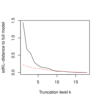
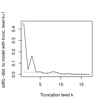
Figure 8: Visualization of the algorithms for the 19-dimensional Norwegian finance data.
Left (Algorithm 1): sdKL-distance to full model with dashed bootstrapped 95% confidence bounds.
Right (Algorithm 2): sdKL-distance to model with truncation level $k+1$ with dashed bootstrapped 95% confidence bounds.

We see that the sdKL-distance to the full model is rapidly decreasing in the truncation level $k$, being quite close to the 95% confidence bound for $k\geq 4$, very close for $k\geq 6$ and dropping below it for $k=10$. Hence we can conclude that the optimal truncation level found by Algorithm 1 is 10, while a truncation level of 6 or even 4 may also be justified if one seeks more parsimonious models. This is exactly in line with the findings of Brechmann et al., (2012), who ascertained that depending on the favored degree of parsimony both truncation levels 4 and 6 may be justified. Yet, they find that there still are significant dependencies beyond the sixth tree. This can also be seen from the right plot of Figure 8, which visualizes the results from Algorithm 2. We see that the distance between two subsequent truncated vines first falls below the 95% confidence bound for $k=6$, after being close to it for $k=4$ and $k=5$. Thus we see that in this example Algorithm 2 indeed finds a more parsimonious model than Algorithm 1. If we took the distances between all subsequent truncated vines into account, we would see that trees 9 and 10 still contribute significant dependencies, such that the “global” optimal truncation level again would be 10. If a data analyst decided that the parsimonious model truncated at level 6 or 4 would suffice for modeling this 19-dimensional data set, he or she would be able to reduce the number of pair-copulas to be modeled from 171 of the full model to 93 or 66, respectively, and thus greatly improve model interpretation and simplify further computations involving the model (e.g. Value-at-Risk simulations).

52-dimensional EuroStoxx50 data

Since the positive effect of truncating vine copulas intensifies with increasing dimensions, we revisit the 52-dimensional EuroStoxx50 data set from Section 3.2. For risk managers it is an relevant task to correctly assess the interdependencies between these variables since they are included in most international banking portfolios. Figure 9 shows the results of the algorithms for this data set.

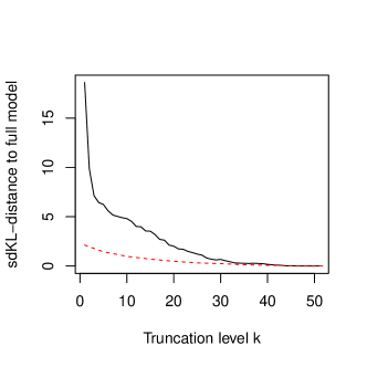
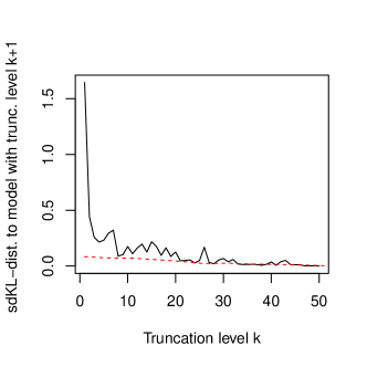
Figure 9: Visualization of the algorithms for the 52-dimensional EuroStoxx50 data.
Left (Algorithm 1): sdKL-distance to full model with dashed bootstrapped 95% confidence bounds.
Right (Algorithm 2): sdKL-distance to model with truncation level $k+1$ with dashed bootstrapped 95% confidence bounds.

In the left panel we see that most of the dependence is captured by the first few trees since there the sdKL-distance to the full model has its sharpest decrease in truncation level $k$. The distance gets very close to the dashed 95% confidence bound for $k>27$, however crossing it not before $k=43$, implying a rather high truncation level. Considering the visualized results of Algorithm 2 in the right panel of Figure 9 we observe that the distances between subsequent truncated vines is quite small for $k\geq 8$, first dropping below the 95% confidence bound for $k=24$. However, it increases again afterwards and ultimately drops below the confidence bound for $k=44$. One could argue that a truncation level of $k=33$ might be advisable since the treewise distance slightly exceeds the confidence bound only three times thereafter. This would reduce the number of pair-copulas to be modeled from 1326 for the full 52-dimensional model to 1155 for the 33-truncated vine copula. Thus, with the help of model distances we can find simpler models for high-dimensional data.

For comparison, the algorithm from Brechmann et al., (2012) finds optimal truncation levels of 47 (without correction), 24 (AIC correction) and 3 (BIC correction). We see that there are large differences between the three methods: Whereas a truncation level of 47 corresponds almost to the non-truncated vine, one should be skeptical whether a 3-truncated vine is apt to describe the dependence structure of 52 random variables.

6 Conclusion

Vine copulas are a state-of-the-art method to model high-dimensional copulas. The applications presented in this paper show the necessity of calculating distances between such high-dimensional vine copulas. In essence, whenever we have more than one vine model to describe observed data, be it a simplified and a non-simplified vine, vines with different truncation levels or with certain restrictions on pair-copula families or the underlying vine structure, model distances help to select the best out of the candidate models. The modifications of the Kullback-Leibler distance introduced in Killiches et al., 2017b have proven to be fast and accurate even in high dimensions, where the numerical calculation of the KL is infeasible. While in this paper we only considered datasets with dimensions $d\leq 52$, applications in even higher dimensions are possible. With the theory developed in Müller and Czado, (2017) the fitting of vines with hundreds of dimensions is facilitated with the focus on sparsity, i.e. fitting as many independence copulas as justifiable in order to reduce the number of parameters. In ongoing research the proposed distance measures are applied to select between several of these high-dimensional models.

References

- Aas et al., (2009) Aas, K., Czado, C., Frigessi, A., and Bakken, H. (2009). Pair-copula constructions of multiple dependence. Insurance, Mathematics and Economics, 44:182–198.
- Acar et al., (2012) Acar, E. F., Genest, C., and Nešlehová, J. (2012). Beyond simplified pair-copula constructions. Journal of Multivariate Analysis, 110:74–90.
- Akaike, (1998) Akaike, H. (1998). Information theory and an extension of the maximum likelihood principle. In Selected Papers of Hirotugu Akaike, pages 199–213. New York, NY: Springer.
- Bedford and Cooke, (2002) Bedford, T. and Cooke, R. M. (2002). Vines: A new graphical model for dependent random variables. Annals of Statistics, 30:1031–1068.
- Brechmann and Czado, (2013) Brechmann, E. C. and Czado, C. (2013). Risk management with high-dimensional vine copulas: An analysis of the Euro Stoxx 50. Statistics & Risk Modeling, 30(4):307–342.
- Brechmann et al., (2012) Brechmann, E. C., Czado, C., and Aas, K. (2012). Truncated regular vines in high dimensions with application to financial data. Canadian Journal of Statistics, 40(1):68–85.
- Brechmann and Joe, (2015) Brechmann, E. C. and Joe, H. (2015). Truncation of vine copulas using fit indices. Journal of Multivariate Analysis, 138:19–33.
- Casella and Berger, (2002) Casella, G. and Berger, R. L. (2002). Statistical inference, volume 2. Pacific Grove, CA: Duxbury.
- Chen and Fan, (2005) Chen, X. and Fan, Y. (2005). Pseudo-likelihood ratio tests for semiparametric multivariate copula model selection. Canadian Journal of Statistics, 33(3):389–414.
- Chen and Fan, (2006) Chen, X. and Fan, Y. (2006). Estimation and model selection of semiparametric copula-based multivariate dynamic models under copula misspecification. Journal of econometrics, 135(1):125–154.
- Cook and Johnson, (1986) Cook, R. and Johnson, M. (1986). Generalized burr-pareto-logistic distributions with applications to a uranium exploration data set. Technometrics, 28(2):123–131.
- Cover and Thomas, (2012) Cover, T. M. and Thomas, J. A. (2012). Elements of information theory. Hoboken, NJ: John Wiley & Sons.
- Czado, (2010) Czado, C. (2010). Pair-copula constructions of multivariate copulas. In Jaworski, P., Durante, F., Härdle, W. K., and Rychlik, T., editors, Copula theory and its applications, chapter 4, pages 93–109. New York, NY: Springer.
- Demarta and McNeil, (2005) Demarta, S. and McNeil, A. J. (2005). The t copula and related copulas. International statistical review, 73(1):111–129.
- Diks et al., (2010) Diks, C., Panchenko, V., and Van Dijk, D. (2010). Out-of-sample comparison of copula specifications in multivariate density forecasts. Journal of Economic Dynamics and Control, 34(9):1596–1609.
- Dißmann et al., (2013) Dißmann, J., Brechmann, E. C., Czado, C., and Kurowicka, D. (2013). Selecting and estimating regular vine copulae and application to financial returns. Computational Statistics & Data Analysis, 59:52–69.
- Efron and Tibshirani, (1994) Efron, B. and Tibshirani, R. J. (1994). An introduction to the bootstrap. Boca Raton, FL: CRC press.
- Genest and Rémillard, (2008) Genest, C. and Rémillard, B. (2008). Validity of the parametric bootstrap for goodness-of-fit testing in semiparametric models. In Annales de l’IHP Probabilités et statistiques, volume 44, pages 1096–1127.
- Hobæk Haff et al., (2010) Hobæk Haff, I., Aas, K., and Frigessi, A. (2010). On the simplified pair-copula construction — simply useful or too simplistic? Journal of Multivariate Analysis, 101(5):1296–1310.
- Joe, (1997) Joe, H. (1997). Multivariate models and multivariate dependence concepts. Boca Raton, FL: CRC Press.
- Joe, (2006) Joe, H. (2006). Generating random correlation matrices based on partial correlations. Journal of Multivariate Analysis, 97(10):2177–2189.
- Joe, (2014) Joe, H. (2014). Dependence modeling with copulas. Boca Raton, FL: CRC Press.
- (23) Killiches, M., Kraus, D., and Czado, C. (2017a). Examination and visualisation of the simplifying assumption for vine copulas in three dimensions. Australian & New Zealand Journal of Statistics, 59(1):95–117.
- (24) Killiches, M., Kraus, D., and Czado, C. (2017b). Model distances for vine copulas in high dimensions. Statistics and Computing, pages 1–19.
- Kullback and Leibler, (1951) Kullback, S. and Leibler, R. A. (1951). On information and sufficiency. The annals of mathematical statistics, 22:79–86.
- Müller and Czado, (2017) Müller, D. and Czado, C. (2017). Representing sparse Gaussian DAGs as sparse R-vines allowing for non-Gaussian dependence. arXiv preprint arXiv:1604.04202.
- Nelsen, (2006) Nelsen, R. (2006). An introduction to copulas, 2nd. New York, NY: Springer Science+Business Media.
- Rosenblatt, (1952) Rosenblatt, M. (1952). Remarks on a multivariate transformation. Ann. Math. Statist., 23(3):470–472.
- Schepsmeier et al., (2017) Schepsmeier, U., Stöber, J., Brechmann, E. C., Gräler, B., Nagler, T., and Erhardt, T. (2017). VineCopula: Statistical inference of vine copulas. R package version 2.1.1.
- Schwarz, (1978) Schwarz, G. (1978). Estimating the dimension of a model. The annals of statistics, 6(2):461–464.
- Sklar, (1959) Sklar, A. (1959). Fonctions dé repartition á n dimensions et leurs marges. Publications de l’Instutut de Statistique de l’Université de Paris, 8:229–231.
- Spanhel and Kurz, (2015) Spanhel, F. and Kurz, M. S. (2015). Simplified vine copula models: Approximations based on the simplifying assumption. arXiv preprint arXiv:1510.06971.
- Stöber and Czado, (2012) Stöber, J. and Czado, C. (2012). Pair copula constructions. In Mai, J. F. and Scherer, M., editors, Simulating Copulas: Stochastic Models, Sampling Algorithms, and Applications, chapter 5, pages 185–230. Singapore, SG: World Scientific.
- Stöber and Czado, (2014) Stöber, J. and Czado, C. (2014). Regime switches in the dependence structure of multidimensional financial data. Computational Statistics & Data Analysis, 76:672–686.
- Stöber et al., (2013) Stöber, J., Joe, H., and Czado, C. (2013). Simplified pair copula constructions – limitations and extensions. Journal of Multivariate Analysis, 119:101–118.
- Vatter, (2016) Vatter, T. (2016). gamCopula: Generalized additive models for bivariate conditional dependence structures and vine copulas. R package version 0.0-1.
- Vatter and Nagler, (2016) Vatter, T. and Nagler, T. (2016). Generalized additive models for pair-copula constructions. Available at SSRN 2817949.