Measuring Fairness in Ranked Outputs

Abstract

Ranking and scoring are ubiquitous. We consider the setting in which an institution, called a ranker, evaluates a set of individuals based on demographic, behavioral or other characteristics. The final output is a ranking that represents the relative quality of the individuals. While automatic and therefore seemingly objective, rankers can, and often do, discriminate against individuals and systematically disadvantage members of protected groups. This warrants a careful study of the fairness of a ranking scheme.

In this paper we propose fairness measures for ranked outputs. We develop a data generation procedure that allows us to systematically control the degree of unfairness in the output, and study the behavior of our measures on these datasets. We then apply our proposed measures to several real datasets, and demonstrate cases of unfairness. Finally, we show preliminary results of incorporating our ranked fairness measures into an optimization framework, and show potential for improving fairness of ranked outputs while maintaining accuracy.

1 Introduction

Ranking and scoring are ubiquitous. We consider the setting in which an institution, called a ranker, evaluates a set of items (typically individuals, but also colleges, restaurants, websites, products, etc) based on demographic, behavioral or other characteristics. The output is a ranking representing the relative quality of the items.

Rankings are used as the basis of important decisions including college admissions, hiring, promotion, grant making, and lending. As a result, rankings have a potentially enormous impact on the livelihood and well-being of individuals. While automatic and therefore seemingly objective, rankers can discriminate against individuals and systematically disadvantage members of protected groups [3]. This warrants a careful study of the fairness of a ranking scheme, a topic we investigate in this paper.

A useful dichotomy is between individual fairness — a requirement that similar individuals are treated similarly, and group fairness, also known as statistical parity — a requirement that demographics of those receiving a particular positive outcome are identical to the demographics of the population as a whole [4]. The focus of this paper is on statistical parity, and in particular on the case where a subset of the population belongs to a protected group. Members of a protected group share a characteristic that cannot be targeted for discrimination. In the US, such characteristics include race, gender and disability status, among others.

We make a simplifying assumption and consider membership in one protected group at a time (i.e., we consider only gender or disability status or membership in a minority group). Further, we assume that membership in a protected group is binary (minority vs. majority group, rather than a break-down by ethnicity). This is a reasonable starting point, and is in line with much recent literature [4, 9, 10].

In this paper we propose several measures that quantify statistical parity, or lack thereof, in ranked outputs. The reasons to consider this problem are two-fold. First, having insight into the properties of a ranked output, or more generally of an output of an algorithmic process, helps make the process transparent, interpretable and accountable [6, 8]. Second, principled fairness quantification mechanisms allow us to engineer better algorithmic rankers, correcting for bias in the input data that is due to the effects of historical discrimination against members of protected groups.

To reason about fair assignment of outcomes to groups, we must first understand the meaning of a positive outcome in our context. There is a large body of work on measuring discrimination in machine learning, see [10] for a survey. The most commonly considered algorithmic task is binary classification, where items assigned to the positive class are assumed to receive the positive outcome. In contrast to classification, a ranking is, by definition, relative, and so outcomes for items being ranked are not strictly positive or negative. The outcome for an item ranked among the top-5 is at least as good as the outcome for an item ranked among the top-10, which is in turn at least as good as the outcome for an item ranked among the top-20, etc.

Basic idea. Our formulation of fairness measures is based on the following intuition: Because it is more beneficial for an item to be ranked higher, it is also more important to achieve statistical parity at higher ranks. The idea is to take several well-known statistical parity measures proposed in the literature [10], and make them rank-aware by placing them within the nDCG framework [5]. nDCG is commonly used for evaluating the quality of ranked lists in information retrieval, and is appropriate here because it provides a principled weighted discount mechanism. Specifically, we calculate set-wise parity at a series of cut-off points in a ranking, and progressively sum these values with a position-based discount.

The rest of this paper is organized as follows. We fix our notation and describe a procedure for generating synthetic rankings of varying degrees of fairness in Section 2. In Section 3 we present novel ranked fairness measures and show their behavior on synthetic and real datasets. In Section 4 we show that fairness in rankings can be improved through an optimization framework, but that additional work is needed to integrate the fairness and accuracy measures into the framework more tightly, to achieve better performance. We conclude in Section 5.

2 Preliminaries

We are given a database $I(\underline{k},s,x_{1},\ldots,x_{m})$ of items. In this database, an item identified by $k$ is associated with an attribute $s$ that denotes membership in a binary protected group, and with descriptive attributes $x_{1},\ldots,x_{m}$. We denote by $S^{+}\subseteq I$ the items that belong to the protected group, and by $S^{-}=I\setminus S^{+}$ the remaining items.

A ranking over $I$ is a bijection $\boldsymbol{\tau}:I\rightarrow\{1,\ldots,N\}$, where $\boldsymbol{\tau}(k)$ is the position of the item with identifier $k$ in $\boldsymbol{\tau}$. We refer to the item at position $i$ in $\boldsymbol{\tau}$ by $\tau_{i}$. For a pair of items $k_{1},k_{2}$, we say that $k_{1}$ is preferred to $k_{2}$ in $\boldsymbol{\tau}$, denoted $k_{1}\succ_{\boldsymbol{\tau}}k_{2}$ if $\boldsymbol{\tau}(k_{1})<\boldsymbol{\tau}(k_{2})$. Figure 1 gives an example of rankings of individuals, with gender as the protected attribute.

We denote by $\boldsymbol{\tau}_{1..i}$ the top-$i$ portion of $\boldsymbol{\tau}$, and by $S^{+}_{1\ldots i}$ the items from the protected group $S^{+}$ that appear among the top-$i$: $S^{+}\cap\boldsymbol{\tau}_{1..i}$.

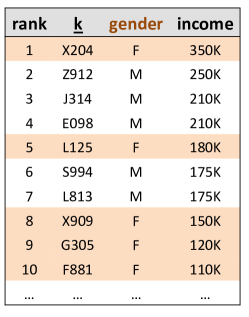
Figure 1: A ranked list, sorted in descending order of income, $gender=F$ is protected.

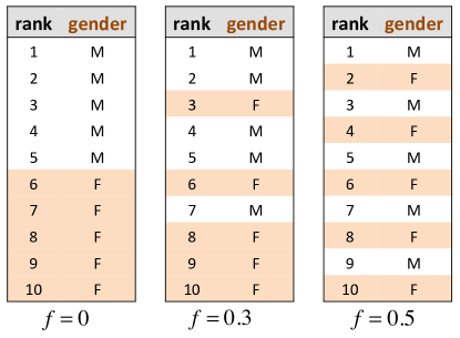
Figure 2: Three ranked lists, $gender=F$ is the protected group.

Data generator

To systematically study the behavior of the proposed measures, we generate synthetic ranked datasets of varying degrees of fairness. Algorithm 1 presents our data generation procedure. This algorithm takes two inputs. The first is a ranking $\boldsymbol{\tau}$, which may be a random permutation of the items in $I$, or it may be generated by the vendor according to their usual process, e.g., in a score-based manner. The second input is the fairness probability $f\in[0,1]$, which specifies the relative preference between items in $S^{+}$ and in $S^{-}$. When $f=0.5$, groups $S^{+}$ and $S^{-}$ are mixed in equal proportion for as long as there are items in both groups. When $f>0.5$, members of $S^{+}$ are preferred, and when $f<0.5$ members of $S^{-}$ are preferred. In extreme cases, when $f=0$, all members of $S^{-}$ will be placed in the output ranking $\boldsymbol{\sigma}$ before any members of $S^{+}$ (first all male individuals, then all female in Figure 1); when $f=1$, the opposite will be true: all of $S^{+}$ will be ranked higher than $S^{-}$ in the output $\boldsymbol{\sigma}$.

The following additional property holds for a pair $k_{1},k_{2}\in I$: if $(k_{1}.s=k_{2}.s)\wedge(k_{1}\succ_{\boldsymbol{\tau}}k_{2})$ then $k_{1}\succ_{\boldsymbol{\sigma}}k_{2}$. That is, Algorithm 1 does not change the relative order among a pair of items that are both in $S^{+}$ or in $S^{-}$.

Algorithm 1 Unfair ranking generator

0:  Ranking $\boldsymbol{\tau}$, fairness probability $f$.{Initialize the output ranking $\boldsymbol{\sigma}$.}

1:  $\boldsymbol{\sigma}\leftarrow\emptyset$

2:  $\boldsymbol{\tau}^{+}=\boldsymbol{\tau}\cap S^{+}$

3:  $\boldsymbol{\tau}^{-}=\boldsymbol{\tau}\cap S^{-}$

4:  while $(\boldsymbol{\tau}^{+}\neq\emptyset)\wedge(\boldsymbol{\tau}^{-}\neq\emptyset)$ do

5:     $p=random([0,1])$

6:     if $p<f$ then

7:        $\boldsymbol{\sigma}\leftarrow pop(\boldsymbol{\tau}^{+})$

8:     else

9:        $\boldsymbol{\sigma}\leftarrow pop(\boldsymbol{\tau}^{-})$

10:     end if

11:  end while

12:  $\boldsymbol{\sigma}\leftarrow\boldsymbol{\tau}^{+}$

13:  $\boldsymbol{\sigma}\leftarrow\boldsymbol{\tau}^{-}$

14:  return  $\boldsymbol{\sigma}$

Figure 2 gives examples of three ranked lists of 10 individuals, with the specified fairness probabilities, and with $gender=F$ as the protected group. For $f=0$, all male individuals are placed ahead of the females. For $f=0.3$, males and females are mixed, but males occur more frequently at top ranks. For $f=0.5$, males and females are mixed in equal proportion.

3 Fairness measures

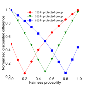
Figure 3: rND on 1,000 items

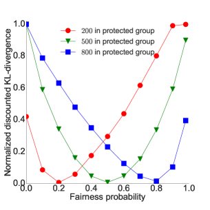
Figure 4: rKL on 1,000 items

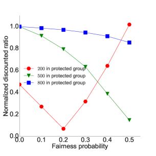
Figure 5: rRD on 1,000 items

A ranking scheme exhibits statistical parity if membership in a protected group does not influence an item’s position in the output. We now present three measures of statistical parity that capture this intuition.

Our measures quantify the relative representation of the protected group $S^{+}$ in a ranking $\boldsymbol{\tau}$. For all measures, we compute set-based fairness at discrete points in the ranking (top-$10$, top-$20$, etc), and compound these values with a logarithmic discount. In this way, we express that higher positions in the ranking are more important, i.e., that it is more important to be fair at the top-$10$ than at the top-$100$. Our logarithmic discounting method is inspired by that used in nDCG [5], a ranked quality measure in Information Retrieval.

All measures presented in this section are normalized to the $[0,1]$ range for ease of interpretation. All measures have their best (most fair) value at 0, and their worst value at 1.

Normalized discounted difference (rND)

Normalized discounted difference (rND) (Equation 1), computes the difference in the proportion of members of the protected group at top-$i$ and in the over-all population.

Values are accumulated at discrete points in the ranking with a logarithmic discount, and finally normalized. Normalizer $Z$ is computed as the highest possible value of rND for the given number of items $N$ and protected group size $|S^{+}|$.

$$\textsf{rND}(\boldsymbol{\tau})=\frac{1}{Z}\sum_{i=10,20,...}^{N}{\frac{1}{log_{2}{i}}\left|\frac{|S^{+}_{1\ldots i}|}{i}-\frac{|S^{+}|}{N}\right|}$$ (1)

Figure 5 plots the behavior of rND on synthetic datasets of 1000 items, with 200, 500 and 800 items in $S^{+}$, as a function of fairness probability. We make four observations: (1) Groups $S^{+}$ and $S^{-}$ are treated symmetrically — a low proportion of either $S^{+}$ or $S^{-}$ at high ranks leads to a high (unfair) rND score. (2) The best (lowest) value of rND is achieved when fairness parameter is set to the value matching the proportion of $S^{+}$ in $I$: 0.2 for 200 protected group members out of 1000, 0.5 for 500 members, and 0.8 for 800 members. (3) rND is convex and continuous. (4) rND is not differentiable at 0.

We argued in the introduction that fairness measures are important not only as a means to observe properties of the output, but also because they allow us to engineer processes that are more fair. A common approach is to specify an optimization problem in which some notion of accuracy or utility is traded against some notion of fairness [9]. While rND presented above is convex and continuous, it is not differentiable, limiting its usefulness in an optimization framework. This consideration motivates us to develop an alternative measure, rKL, described next.

Normalized discounted KL-divergence (rKL)

Kullback-Leibler (KL) divergence measures the expectation of the logarithmic difference between two discrete probability distributions $P$ and $Q$:

$$D_{KL}(P||Q)=\sum_{i}P(i)log\frac{P(i)}{Q(i)}$$ (2)

We use KL-divergence to compute the expectation of the difference between protected group membership at top-$i$ vs. in the over-all population. We take:

$$P=\left(\frac{|S^{+}_{1\ldots i}|}{i},\frac{|S^{-}_{1\ldots i}|}{i}\right),Q=\left(\frac{|S^{+}|}{N},\frac{|S^{-}|}{N}\right)$$ (3)

and define normalized discounted KL-divergence (rKL) as:

$$\textsf{rKL}(\boldsymbol{\tau})=\frac{1}{Z}\sum_{i=10,20,...}^{N}{\frac{D_{KL}(P||Q)}{log_{2}{i}}}$$ (4)

Figure 5 plots the behavior of rKL on synthetic datasets of 1000 items, with 200, 500 and 800 items in $S^{+}$, as a function of fairness probability. We observe that this measure has similar behavior as rND (Equation 1 and Figure 1), but that it appears smoother, and so may be more convenient to optimize robustly. An additional advantage of rKL is that it can be used without modification to go beyond binary protected group membership, e.g., to capture proportions of different racial groups, or age groups, in a population.

Normalized discounted ratio (rRD)

Our final measure, normalized discounted ratio (rRD), is formulated similarly to rND, with the difference in the denominator of the fractions: the size of $S^{+}_{1\ldots i}$ is compared to the size of $S^{-}_{1\ldots i}$, not to $i$ (and similarly for the second term, $S^{+}$). When either the numerator or the denominator of a fraction is 0, we set the value of the fraction to 0.

Behavior of the rRD measure on a synthetic dataset is presented in Figure 5. We observe that rRD reaches its best (lowest) value at the same points as do rND and rKL, but that it shows different trends. Most importantly, because rRD does not treat $S^{+}$ and $S^{-}$ symmetrically, its behavior when protected group represents the majority of the over-all population (800 protected group members out of 1000 in Figure 5), or when $S^{+}$ is preferred to $S^{-}$ (fairness probability $>0.5$), is not meaningful. We conclude that rRD is only applicable when the protected group is the minority group, i.e., when $S^{+}$ corresponds to at most 50% of the underlying population, and when fairness probability is below 0.5.

$$\textsf{rRD}(\boldsymbol{\tau})=\frac{1}{Z}\sum_{i=10,20,...}^{N}{\frac{1}{log_{2}{i}}\left|\frac{|S^{+}_{1\ldots i}|}{|S^{-}_{1\ldots i}|}-\frac{|S^{+}|}{|S^{-}|}\right|}$$ (5)

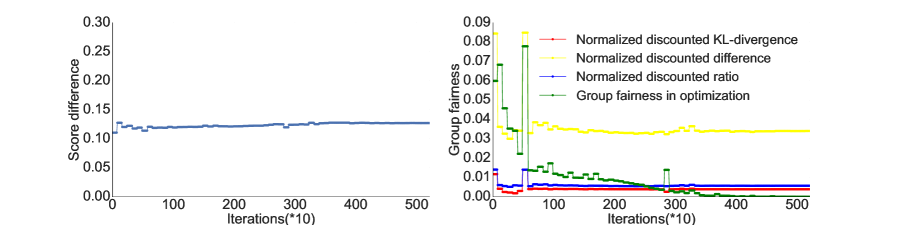
Figure 6: Accuracy and fairness on German Credit, ranked by sum of normalized attribute values, with $k=10$.

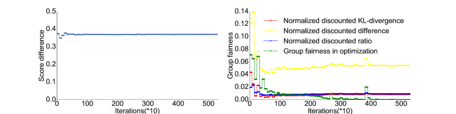
Figure 7: Accuracy and fairness on German Credit, ranked by credit amount, with $k=10$.

Evaluation with real datasets

We used several real datasets to study the relative behavior of our measures, and to see whether our measures signal any fairness violations in that data. We highlight results on two datasets: ProPublica [1] and German Credit [7]. Results on other datasets, including CS Rankings [2], US News & World Report rankings (premium.usnews.com/best-colleges), and Adult Income [7] show interesting trends but we do not include them due to space limitations. These will be discussed in the full version of the paper.

ProPublica is the recidivism data analyzed by [1] and retrieved from https://github.com/propublica/compas-analysis. This dataset contains close to 7,000 criminal defendant records. The goal of the analysis done by [1] was to establish whether there is racial bias in the software that computes predictions of future criminal activity. Racial bias was indeed ascertained, as was gender bias, see [1] for details. In our analysis we set out to check whether ranking on the values of recidivism score, violent recidivism score, and on the number of prior arrests shows parity w.r.t. race (black as the protected group, 51% of the dataset) and gender (female as the protected group, 19% of the dataset).

Using race as the protected attribute, we found rND = 0.44 for ranking on recidivism and rND = 0.44. We found lower but still noticeable rKL values for these rankings (0.17 and 0.18, respectively). Interestingly, ranking by the number of prior arrests produced rND = 0.23 but rKL = 0.04, showing much higher unfairness according to the rND measure than to the rKL. Note that rRD is inapplicable here, since the protected group constitutes the majority of the population.

Using gender as the protected attribute, we found rND = 0.15 for ranking on recidivism score, rND = 0.12 for violent recidivism and rND = 0.11 for ranking on prior arrests. The rKL was low — between 0.01 and 0.02 for these cases. We measured rRD = 0.20 for recidivism ranking, rRD = 0.14 for violent recidivism and rRD = 0.16 for prior arrests.

German Credit is a dataset from [7] with financial information about 1,000 individuals applying for loans. This dataset is typically used for classification tasks. Nonetheless, several of the attributes that are part of this dataset can be used for ranking, including duration (month), credit amount, status of existing account, and employment length. We experimented with ranking on individual attributes duration (months) and credit amount, and also used a score-based ranker that computes the score of each individual by normalizing the value of each attribute, and then summing them with equal weights. We used all attributes that are either continuous or discrete but ordered.

As protected attributes, we used gender (69% female) and age (15% younger than 25, 55% younger than 35). For these cases, rKL ranged between 0.01 and 0.15, and rND ranged between 0.05 and 0.41. rRD was only applicable to age below 25, and ranged between 0.08 and 0.12. We will show in Section 4 results of optimizing fairness for this dataset, with $age<25$ as the protected attribute.

4 Learning fair rankings

In this section we describe an optimization method for improving the fairness of ranked outputs. Our approach is based closely on the fair representations framework of Zemel et. al [9], which focuses on making classification tasks fair. We first briefly describe their framework, and then explain our modifications that make it applicable to rankings.

The main idea in [9] is to introduce a level of indirection between the input space $X$ that represents individuals and the output space $Y$ in which classification outcomes are assigned to individuals. Specifically, they introduce a multinomial random variable $Z$ of size $k$, with each of the $k$ values representing a “prototype” (cluster) in the space of $X$. The goal is to learn a mapping from $X$ to $Z$ that preserves information about attributes that are useful for the classification task at hand, while at the same time hiding information about protected group membership of $x$. Statistical parity in this framework is formulated as $P(Z=k~{}|~{}x\in S^{+})=P(Z=k~{}|~{}x\in S^{-}),\forall k$.

The goal is to learn a mapping that satisfies statistical parity and at the same time preserves utility. For this, $Z$ must be a good description of $X$ (distances from $x\in X$ to its representation in $\hat{x}$ should be small) and predictions based on $\hat{x}$ should be accurate. This formulation gives rise to the following multi-criteria optimization problem, with the loss function $L=A_{x}L_{x}+A_{y}L_{y}+A_{z}L_{z}$, where $L_{x}$, $L_{y}$ and $L_{z}$ are loss functions and $A_{x}$, $A_{y}$, $A_{z}$ are hyper-parameters governing the trade-offs. We keep the terms responsible for statistical parity ($L_{z}$) and distance in the input space ($L_{x}$) as in the original framework, and redefine the term that represents accuracy ($L_{y}$) as appropriate for ranked outcomes. We show here results that use average per-item score difference between the ground-truth ranking $\boldsymbol{\tau}$ and its estimate $\hat{\boldsymbol{\tau}}$ to quantify accuracy. We also experimented with position accuracy (per-item rank difference), Kendall-$\tau$ distance, and Spearman and Pearson’s correlation coefficients, but omit these results due to space limitations, and also because more work is needed to understand convergence properties of the optimization under these measures.

Results of our preliminary evaluation on the German Credit dataset (see Section 3), with $age<25$ as the protected attribute, are presented in Figures 6 (ranked on sum of all attributes, normalized, with equal weights) and 7 (ranked on the credit amount attribute). We show convergence of accuracy (normalized average score difference) and fairness (rND, rKL, rRD, and the statistical parity component $L_{z}$ as “group fairness in optimization”). We observe that all fairness measures converge to a low (fair) value, but that accuracy is optimized more effectively in Figure 6 than in Figure 7, where the score difference is considerable.

5 Conclusions and future work

In this paper we presented novel measures that can be used to quantify statistical parity in rankings. We evaluated these measures in synthetic and real datasets, and showed preliminary optimization results. Much future work remains on the evaluation of these measures — understanding their applicability in real settings, formally establishing their mathematical properties, incorporating them into an optimization framework, and ensuring that the framework is able to both preserve accuracy and improve fairness. One of the bottlenecks in this process is the running time, which we are working to optimize both by looking for ways to make fairness measures more computationally friendly and by careful engineering.

References

- [1] J. Angwin, J. Larson, S. Mattu, and L. Kirchner. Machine bias. ProPublica, May 23, 2016.
- [2] E. Berger. CSRankings: Computer science rankings, 2016.
- [3] D. K. Citron and F. A. Pasquale. The scored society: Due process for automated predictions. Washington Law Review, 89, 2014.
- [4] C. Dwork, M. Hardt, T. Pitassi, O. Reingold, and R. S. Zemel. Fairness through awareness. In Innovations in Theoretical Computer Science 2012, Cambridge, MA, USA, January 8-10, 2012, pages 214–226, 2012.
- [5] K. Järvelin and J. Kekäläinen. Cumulated gain-based evaluation of IR techniques. ACM Trans. Inf. Syst., 20(4):422–446, 2002.
- [6] J. A. Kroll, J. Huey, S. Barocas, E. W. Felten, J. R. Reidenberg, D. G. Robinson, and H. Yu. Accountable algorithms. University of Pennsylvania Law Review, 165, 2017.
- [7] M. Lichman. UCI machine learning repository, 2013.
- [8] J. Stoyanovich and E. P. Goodman. Revealing algorithmic rankers. Freedom to Tinker, August 5, 2016.
- [9] R. S. Zemel, Y. Wu, K. Swersky, T. Pitassi, and C. Dwork. Learning fair representations. In International Conference on Machine Learning, 2013.
- [10] I. Zliobaite. A survey on measuring indirect discrimination in machine learning. CoRR, abs/1511.00148, 2015.