Contextuality as a resource for models of quantum computation on qubits

Abstract

A central question in quantum computation is to identify the resources that are responsible for quantum speed-up. Quantum contextuality has been recently shown to be a resource for quantum computation with magic states for odd-prime dimensional qudits and two-dimensional systems with real wavefunctions. The phenomenon of state-independent contextuality poses a priori an obstruction to characterizing the case of regular qubits, the fundamental building block of quantum computation. Here, we establish contextuality of magic states as a necessary resource for a large class of quantum computation schemes on qubits. We illustrate our result with a concrete scheme related to measurement-based quantum computation.

The model of quantum computation by state injection (QCSI) Bravyi and Kitaev (2005) is a leading paradigm of fault-tolerance quantum computation. Therein, quantum gates are restricted to belong to a small set of classically simulable gates, called Clifford gates Gottesman (1997), that admit simple fault-tolerant implementations Gottesman (1998a). Universal quantum computation is achieved via injection of “magic states” Bravyi and Kitaev (2005), which are the source of quantum computational power of the model.

A central question in QCSI is to characterize the physical properties that magic states need to exhibit in order to serve as universal resources. In this regard, quantum contextuality has recently been established as a necessary resource for QCSI. This was first achieved for quopit systems Veitch et al. (2012); Howard et al. (2014), where the local Hilbert space dimension is an odd prime power, and subsequently for local dimension two with the case of rebits Delfosse et al. (2015). In the latter, the density matrix is constrained to be real at all times.

In this Letter we ask “Can contextuality be established as a computational resource for QCSI on qubits?”. This is not a straightforward extension of the quopit case because the multiqubit setting is complicated by the presence of state-independent contextuality among Pauli observables Mermin (1990a); Peres (1990). Consequently, every quantum state of $n\geq 2$ qubits is contextual with respect to Pauli measurements, including the completely mixed one Howard et al. (2014). It is thus clear that contextuality of magic states alone cannot be a computational resource for every QCSI scheme on qubits.

Yet, there exist qubit QCSI schemes for which contextuality of magic states is a resource, and we identify them in this Letter. Specifically, we consider qubit QCSI schemes ${\cal{M}}_{\cal{O}}$ that satisfy the following two constraints:

1. Resource character. There exists a quantum state that does not exhibit contextuality with respect to measurements available in ${\cal{M}}_{\cal{O}}$.

2. Tomographic completeness. For any state $\rho$, the expectation value of any Pauli observable can be inferred via the allowed operations of the scheme.

The motivation for these constraints is the following.

Condition (C1) constitutes a minimal principle that unifies, simplifies and extends the quopit Howard et al. (2014) and rebit Delfosse et al. (2015) settings. While seemingly a weak constraint, it excludes the possibility of Mermin-type state-independent contextuality Mermin (1990a); Peres (1990) among the available measurements (see Lemma 1 below). A priori, the absence of state-independent contextuality comes at a price. Namely, for any QCSI scheme ${\cal{M}}_{\cal{O}}$ on $n\geq 2$ qubits, not all $n$-qubit Pauli observables can be measured. Thus, the question arises of whether this limits access to all $n$ qubits for measurement. As we show in this Letter, this does not have to be the case.

Addressing this question, we impose tomographic completeness as our technical condition for a “true” $n$-qubit QCSI scheme, cf. (C2). It means that any quantum state can be fully measured given sufficiently many copies. The rebit scheme Delfosse et al. (2015), for example, does not satisfy this.

One of our results is that for any number $n$ of qubits there exists a QCSI scheme that satisfies both conditions (C1) and (C2). The reason why both conditions can simultaneously hold lies in a fundamental distinction between observables that can be measured directly in a given qubit QCSI scheme from those that can only be inferred by measurement of other observables. The resulting qubit QCSI schemes resemble their quopit counterparts Veitch et al. (2012); Howard et al. (2014) in the absence of state-independent contextuality, yet have full tomographic power for the multiqubit setting.

The main result of this Letter is Theorem 1. It says that if the initial (magic) states of a qubit QCSI scheme are describable by a noncontextual hidden variable model (NCHVM) it becomes fundamentally impossible to implement a universal set of gates. We highlight that Theorem 1 applies generally to any scheme fulfilling the condition (C1), including that of Ref. Delfosse et al. (2015).

The condition (C1) plays a pivotal role in our analysis. It is clear that contextuality of the magic states can be a resource only if condition (C1) holds. In this Letter we establish the converse, namely that contextuality of the magic states is a resource for QCSI if condition (C1) holds. Therefore, condition (C1) is the structural element that unifies the previously discussed quopit Howard et al. (2014) and rebit Delfosse et al. (2015) case, and the qubit scenarios discussed here. Together, condition (C1) and Theorem 1 characterize the contextuality types that are needed in quantum computation via state injection, showing that state-dependent contextuality with respect to Pauli observables is a universality resource.

As a final remark, we note that the measurements available in QCSI schemes satisfying (C1) preserve positivity of suitable Wigner functions Raussendorf et al. (2017).

Setting.—An $n$-qubit Pauli observable $T_{a}$ is a hermitian operator with $\pm 1$ eigenvalues of form

$$T_{a}:=\xi{(a)}Z(a_{Z})X(a_{X}):=\xi{(a)}\bigotimes_{i=1}^{n}Z_{i}^{a_{Z_{i}}}\bigotimes_{j=1}^{n}X_{j}^{a_{X_{j}}},$$ (1)

where $a:=(a_{Z},a_{X})$ is a $2n$-bit string and $\xi(a)$ is a phase. Pauli observables define an operator basis that we call $\mathcal{T}_{n}$.

A qubit scheme $\mathcal{M}_{\mathcal{O}}$ of quantum computation via state injection (QCSI) consists of a resource $\mathcal{M}$ of initial “magic” states and 3 kinds of allowed operations:

1. Measurement of any Pauli observable in a set $\mathcal{O}$.

2. A group $G$ of “free” Clifford gates that preserve $\mathcal{O}$ via conjugation up to a global phase.

3. Classical processing and feedforward.

Adaptive circuits of operations 1-3 may be combined with classical postprocessing in order to simulate measurements of Pauli observables that are not in $\mathcal{O}$ (cf. Fig. 1). We name the latter “inferable” and let $\mathcal{I}$ be the superset of $\mathcal{O}$ defined by them. Analogously, we let $\mathcal{J}$ be the set of sets of compatible Pauli observables that can be inferred jointly, which define the “contexts” of our computational model. As shown in Fig.  1, not every set of compatible Pauli observables is necessarily in $\mathcal{J}$. Yet, $A\in\mathcal{I}$ implies that $\{A\}\in\mathcal{J}$. Furthermore, for any pair of observables $\{A,B\}\in\mathcal{J}$ and $\alpha\in\mathbb{R}$, the observables $AB$, $\alpha A$ can be inferred jointly by measuring $A,B$, since the eigenvalues of the latter determine those of the former. Hence,

$$\{A,B\}\in\mathcal{J}\quad\Rightarrow\quad\{A,B,AB,\alpha A\}\in\mathcal{J},\,\,\,\forall\alpha\in\mathbb{R}.$$ (2)

Constraint (C2) holds if and only if $\mathcal{T}_{n}\subset\mathcal{I}$, i.e., if and only if the outcome distribution of any Pauli observable can be sampled via measurements in $\mathcal{O}$ and classical postprocessing.

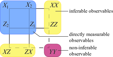
Figure 1: We consider an example scheme $\mathcal{M}_{\mathcal{O}}$ on two qubits with $\mathcal{O}=\{X_{1},X_{2},Z_{1},Z_{2}\}$. Straight lines connect maximal sets of jointly inferable observables. Here, the correlator $X_{1}X_{2}$ ($Z_{1}Z_{2}$) is not in $\mathcal{O}$ but can be inferred by measuring $X_{1},X_{2}$ ($Z_{1},Z_{2}$) and multiplying their outcomes. (This scheme is reminiscent of the syndrome measurement of subsystem codes Poulin (2005).) Yet, $X_{1}X_{2}$ cannot be inferred jointly with $Z_{1}Z_{2}$ because a forbidden measurement of $X_{1},X_{2},Z_{1},Z_{2}$ would be required to reproduce all quantum correlations, but after measuring, e.g., $Z_{1}$ and $Z_{2}$ to infer $Z_{1}Z_{2}$ the outcome statistics of $X_{1}X_{2}$ become uniformly random. Similarly, $X_{1}Z_{2}$ and $Z_{1}X_{2}$ can be separately inferred but not jointly. Further, $YY$ cannot be inferred (observables in $\mathcal{O}$ cannot distinguish its eigenstates).

Contextuality.—Above, imposing (C1) means that there exists a quantum state $\rho$ whose measurement statistics can be reproduced by a noncontextual hidden variable model (NCHVM), which we introduce next.

Definition 1.

A NCHVM $(\mathcal{S},q_{\rho},\Lambda)$ for the state $\rho$ with respect to a scheme $\mathcal{M}_{\mathcal{O}}$ consists of a probability distribution $q_{\rho}$ over a set $\mathcal{S}$ of internal states and a set $\Lambda=\{\lambda_{\nu}\}_{\nu\in\mathcal{S}}$ of value assignment functions $\lambda_{\nu}:\mathcal{I}\rightarrow\{\pm 1\}$ that fulfill:

For any $\lambda_{\nu}\in\Lambda$ and $M\in\mathcal{J}$ the real numbers $\displaystyle\{\lambda_{\nu}(A)\}_{A\in M}$ are compatible eigenvalues: i.e.  there exists a quantum state $|{\psi}\rangle$ such that

$$A|{\psi}\rangle=\lambda_{\nu}(A)|{\psi}\rangle,\quad\forall A\in M.$$ (3)

The distribution $q_{\rho}$ satisfies

$$\langle A\rangle_{\rho}=\mathrm{tr}(A\rho)=\sum_{\nu\in\mathcal{S}}\lambda_{\nu}(A)q_{\rho}(\nu),\quad\forall A\in\mathcal{I}$$ (4)

The state $\rho$ is said to be “contextual” or to “exhibit contextuality” if no NCHVM with respect to $\mathcal{M}_{\mathcal{O}}$ exists.

Qubit QCSI for which all possible inputs exhibit contextuality are forbidden by (C1). Specifically, in this Letter, $\mathcal{O}$ must be a strict subset of $\mathcal{T}_{n}$.

Main result.—We now establish contextuality as a resource for quantum computational universality for all qubit QCSI schemes that fulfill (C1). Below, we call a scheme $\mathcal{M}_{\mathcal{O}}$ universal if for any integer $n\geq 1$ and $V\in U(2^{n})$ there exists a finite-size circuit of $\mathcal{M}_{\mathcal{O}}$ operations that prepares the $n$-qubit state $V|{0}\rangle$ up to any positive trace-norm error.

Theorem 1.

A qubit QCSI scheme $\mathcal{M}_{\mathcal{O}}$ satisfying (C1) is universal for $n\geq 3$ qubits only if its magic states exhibit contextuality.

Theorem 1 applies even in the setting where the computation happens in an encoded subspace, reproducing the rebit results of Ref. Delfosse et al. (2015). We provide a general proof of this fact in a companion paper Raussendorf et al. (2017) and show it here in the encoding-free scenario under an additional assumption, denoted ($\star$), that every qubit must be measurable in at least two complementary Pauli bases. This requirement enforces $\mathcal{M}_{\mathcal{O}}$ to exhibit the phenomenon of quantum complementarity and simplifies our main argument while preserving its core structure.

The proof of theorem 1 relies on a characterization of noncontextual hidden variable models for qubit QCSIs. We make three key observations about such models.

First, by applying Def. 1.(i) to $M:=\{A,B,AB,\alpha A\}\in\mathcal{J}$ as in Eq. (2), we derive two constraints

$$\lambda_{\nu}(AB)=\lambda_{\nu}(A)\lambda_{\nu}(B),\quad\lambda_{\nu}(\alpha A)=\alpha\lambda_{\nu}(A),$$ (5)

that any $\lambda_{\nu}\in\Lambda$ must fulfill for any pair $\{A,B\}\in\mathcal{J},\alpha\in\mathbb{R}$.

Second, we prove the following lemma.

Lemma 1.

For any QCSI scheme $\mathcal{M}_{\mathcal{O}}$ fulfilling (C1) the phase $\xi{(a)}$ in Eq. (1) can be chosen w.l.o.g. so that

$$T_{a}T_{b}=T_{a+b}\quad\textnormal{for any triple $\{T_{a},T_{b},T_{a}T_{b}\}\in\mathcal{J}$}.$$ (6)

Proof.

Let $\xi$ be given and let $\lambda_{\nu}$ be a consistent value assignment for the scheme $\mathcal{M}_{\mathcal{O}}$. W.l.o.g., we can redefine $\mathcal{T}_{n}^{\prime}:=\{T_{a}^{\prime}:=\lambda_{\nu}(T_{a})T_{a},T_{a}\in\mathcal{T}_{n}\}$ and $\mathcal{O^{\prime}}=\{T_{a}^{\prime},T_{a}\in\mathcal{O}\}$ introducing a classical relabeling of measurement outcomes, without changing any quantum feature of the scheme. Using $T_{a+b}=\pm T_{a}T_{b}$, we obtain

$$T_{a+b}^{\prime}={\lambda_{\nu}(T_{a+b})}T_{a+b}={\lambda((\pm 1)T_{a}T_{b})}(\pm 1)T_{a}T_{b}$$

$$\stackrel{{\scriptstyle(\ref{eq:LinearityOfAssignments})}}{{=}}(\pm 1)^{2}{\lambda(T_{a}T_{b})}T_{a}T_{b}\stackrel{{\scriptstyle(\ref{eq:LinearityOfAssignments})}}{{=}}{\lambda(T_{a})}T_{a}{\lambda(T_{b})}T_{b}=T_{a}^{\prime}T_{b}^{\prime}.\>\>\>\>\,\,\qed$$

Last, we observe that for any $M\in\mathcal{J}$, $|{\psi}\rangle$ as in Eq. (3) and $T_{b}\in\mathcal{T}_{n}$, the state $T_{b}|{\psi}\rangle$ is a joint eigenstate of $M$:

$$(\gamma T_{a})T_{b}|{\psi}\rangle=\left(\lambda_{\nu}(\gamma T_{a})(-1)^{[a,b]}\right)T_{b}|{\psi}\rangle,\,\forall\gamma T_{a}\in M,$$ (7)

where $[a,b]:=a_{X}b_{Z}+a_{Z}b_{X}\bmod 2$; combined with Eq. (5), this induces a group action of $\mathbb{Z}_{2}^{2n}$ on value assignments

$$\lambda_{\nu}\quad\stackrel{{\scriptstyle u}}{{\rightarrow}}\quad\lambda_{\nu+u}(T_{a}):=\lambda_{\nu}(T_{a})(-1)^{[u,a]},\;\forall u\in V.$$ (8)

With these tools, we arrive at a powerful intermediate result, namely, a method to construct NCHVMs that can simulate qubit QCSIs on noncontextual inputs.

Lemma 2.

For any qubit scheme $\mathcal{M}_{\mathcal{O}}$ fulfilling (C1) and any quantum circuit $\mathcal{C}$ of $\mathcal{M}_{\mathcal{O}}$ operations, if there exists a NCHVM $(\mathcal{S},q_{\rho_{\text{in}}},\Lambda)$ for some given input state $\rho_{\text{in}}$, there then exists a NCHVM $(\mathcal{S},q_{\rho_{\text{out}}},\Lambda)$ for the output $\rho_{\text{out}}:=\mathcal{C}(\rho_{\text{in}})$.

Lemma 2 establishes that contextuality cannot be freely generated in qubit QCSI. A surprising aspect of this fact is that it holds for circuits that contain intermediate measurements. Intuitively, unitary gates in $\mathcal{G}$ must induce an action on the set of noncontextual states since they preserve the set $\mathcal{O}$. However, the evolution of noncontextual states under measurement is far from intuitive since the latter can often prepare states that are inaccessible to gates Bermejo-Vega and Van Den Nest (2014).

Lemma 2 leads to a simple classical random-walk algorithm for sampling from the output distribution of all measurements in $\mathcal{C}$, which is further efficient if oracles for sampling from $q_{\rho_{\text{in}}}$ and computing any $\lambda_{\nu}\in\Lambda$ are given. The random walk first samples a state $\nu_{0}\in\mathcal{S}$ from $q_{\rho_{\text{in}}}$ and, upon measurement of $T_{a_{t}}\in\mathcal{O}$ at time $t$, outputs $\lambda_{\nu_{t}}(T_{a_{t}})$ given $\nu_{t}$ and updates $\nu_{t}\rightarrow\nu_{t}+a$ with $1/2$ probability. The correctness of this algorithm follows from Eq. (9) below and is analyzed in detailed in Ref. Raussendorf et al. (2017).

Proof.

We fix a phase convention for $T_{a}$ so that Eq. (6) in Lemma 1 holds and introduce a simplified notation

$$\lambda_{\nu}(a):=\lambda_{\nu}(T_{a}),\quad\textnormal{where }T_{a}\in\mathcal{I},a\in\mathbb{Z}_{2}^{2n}.$$

Because free unitaries preserve $\mathcal{O}$ they can be propagated out of $\mathcal{C}$ via conjugation. Hence, we can w.l.o.g. assume that $\mathcal{C}$ consists only of measurements. Our proof is by induction. At time $t=1$, $\rho_{1}=\rho_{\text{in}}$ has an NCHVM by assumption. At any other time $t+1$, given an NCHVM $(\mathcal{S},q_{\rho_{t}},\Lambda)$ for the state $\rho_{t}$, we construct an NCHVM $(\mathcal{S},q_{\rho_{t+1}},\Lambda)$ for $\rho_{t+1}$. Specifically, let $T_{a_{t}}\in{\mathcal{O}}$ be the observable measured at time $t$ with corresponding outcome $s_{t}\in\{\pm 1\}$, ${s}_{\prec t}:=(s_{1},\ldots,s_{t})$ be the string of prior measurement records, and $p(s_{t}|{s}_{\prec t})$ the conditional probability of measuring $s_{t}$; we will now show that $\rho_{t+1}$ admits the hidden-variable representation

$$q_{\rho_{t+1}}(\nu) :=\frac{\delta_{{s_{t}},\lambda_{\nu}(a_{t})}}{p(s_{t}|{s}_{\prec t})}\frac{q_{\rho_{t}}(\nu)+q_{\rho_{t}}(\nu+a_{t})}{2},\vspace{2mm}$$ (9)

where $p(s_{t}|{s}_{\prec t})$ can be predicted by the HVM, since $2p(s_{t}|{s}_{\prec t})=\left\langle I+{s_{t}}T_{a_{t}}\right\rangle_{\rho_{t}}=\langle I\rangle_{\rho_{t}}+{s_{t}}\langle T_{{a}_{t}}\rangle_{\rho_{t}}$—which are known by the induction promise. Our goal is to show that $(\mathcal{S},q_{\rho_{t+1}},\Lambda)$ predicts the expected value of any $T_{a}\in\mathcal{I}$ measured at time $t+1$. For this, we derive a useful expression,

$$\langle T_{a}\rangle_{\rho_{t+1}}^{\mathrm{HVM}}=\displaystyle{{\sum_{\nu\in{\cal{S}}}}q_{\rho_{t+1}}(\nu)\lambda_{\nu}(a)}\vspace{1mm} \stackrel{{\scriptstyle(\ref{eq:MeasurementUpdate})}}{{=}}\sum_{\nu\in{\cal{S}}}\tfrac{\delta_{{s_{t}},\lambda_{\nu}(a_{t})}q_{\rho_{t}}(\nu)}{2p(s_{t}|{s}_{\prec t})}\lambda_{\nu}(a)+\sum_{\nu\in{\cal{S}}}\tfrac{\delta_{{s_{t}},\lambda_{\nu}(a_{t})}q_{\rho_{t}}(\nu+a_{t})}{2p(s_{t}|{s}_{\prec t})}\lambda_{\nu}(a).$$ (10)

$$\stackrel{{\scriptstyle(\ref{Transl})}}{{=}}\sum_{\nu\in{\cal{S}}}\tfrac{\delta_{{s_{t}},\lambda_{\nu}(a_{t})}q_{\rho_{t}}(\nu)}{2p(s_{t}|{s}_{\prec t})}\lambda_{\nu}(a)+\tfrac{\delta_{{s_{t}},\lambda_{\nu}(a_{t})}q_{\rho_{t}}(\nu)}{2p(s_{t}|{s}_{\prec t})}\lambda_{\nu}(a)(-1)^{[a,a_{t}]},$$

which we evaluate on two cases:

(A) $T_{a},T_{a_{t}}$ anticommute, hence, $[a,a_{t}]=1$. We get $\langle T_{a}\rangle_{\rho_{t+1}}^{\mathrm{HVM}}=0$, in agreement with quantum mechanics.

(B) $T_{a},T_{a_{t}}$ commute. In this case $[a,a_{t}]=0$. Using the identity $\delta_{s,\lambda}=(1+s\lambda)/2,s,\lambda\in\{\pm 1\}$, we obtain

$$\langle T_{a}\rangle_{\rho_{t+1}}^{\mathrm{HVM}}=\sum_{\nu\in{\cal{S}}}\frac{1+{s_{t}}\lambda_{\nu}({a}_{t})}{2p(s_{t}|{s}_{\prec t})}q_{\rho_{t}}(\nu)\lambda_{\nu}(a)$$

$$\displaystyle\stackrel{{\scriptstyle(\ref{eq:LinearityOfAssignments})}}{{=}}\frac{\sum_{\nu\in{\cal{S}}}q_{\rho_{t}}(\nu)\lambda_{\nu}(a)+{s_{t}}\sum_{\nu\in{\cal{S}}}q_{\rho_{t}}(\nu)\lambda_{\nu}(a+a_{t})}{2p(s_{t}|{s}_{\prec t})}$$

Finally, by induction hypothesis, we arrive at

$$\langle T_{a}\rangle_{\rho_{t+1}}^{\mathrm{HVM}} =\displaystyle{\frac{\langle T_{a}\rangle_{\rho_{t}}+{s_{t}}\langle T_{a+a_{t}}\rangle_{\rho_{t}}}{2p(s_{t}|{s}_{\prec t})}}\stackrel{{\scriptstyle(\ref{eq:PauliAdditivity})}}{{=}}\displaystyle{\frac{\text{tr}\left(\rho_{t}\frac{I+{s_{t}}T_{a_{t}}}{2}T_{a}\right)}{p(s_{t}|{s}_{\prec t})}}$$

$$=\displaystyle{\text{tr}\left(\frac{\left[\frac{I+{s_{t}}T_{a_{t}}}{2}\rho_{t}\frac{I+{s_{t}}T_{a_{t}}}{2}\right]}{p(s_{t}|{s}_{\prec t})}T_{a}\right)}=\mathrm{tr}\left(\rho_{t+1}T_{a}\right)$$

which is again the quantum mechanical prediction. ∎

Finally, we prove our main result.

Proof of theorem 1.

We derive a contradiction by assuming (A1) that $\mathcal{M}_{\mathcal{O}}$ is universal and (A2) that all magic states in $\mathcal{M}$ are noncontextual. We first consider the computation to be error-free and drop this assumption at the end.

Recall that, by assumption ($\star$), two complementary Pauli observables, denoted $Z_{i},X_{i}\in\mathcal{O}$ w.l.o.g., can be measured on any qubit. By (A1), the scheme $\mathcal{M}_{\mathcal{O}}$ can prepare the encoded GHZ state $|{\psi}\rangle$ that is uniquely stabilized by $X_{1}X_{2}X_{3}$, $-X_{1}Z_{2}Z_{3}$, $-Z_{1}X_{2}Z_{3}$, $-Z_{1}Z_{2}X_{3}$. Furthermore, $\mathcal{M}_{\mathcal{O}}$ can also infer the value of any correlator of form $A_{1}A_{2}A_{3}$ with $A_{i}\in\{X_{i},Z_{i}\}$ (in particular, $|{\psi}\rangle$’s stabilizers) by measuring $A_{1},A_{2},A_{3}$ individually. Quantum mechanics predicts

$$\left\langle X_{1}X_{2}X_{3}-X_{1}Z_{2}Z_{3}-Z_{1}X_{2}Z_{3}-Z_{1}Z_{2}X_{3}\right\rangle_{\psi}^{\mathrm{QM}}=4.$$

On the other hand, by (A2) and Lemma 2, there exists an NCHVM for $|{\psi}\rangle$ with respect to all quadruples of form $\{A_{1},A_{2},A_{3},A_{1}A_{2}A_{3},A_{i}\in X_{i},Z_{i}\}$. Using constraint (5) for noncontextual value assignments, we derive an inequality for the NCHVM’s prediction

$$\left\langle X_{1}X_{2}X_{3}-X_{1}Z_{2}Z_{3}-Z_{1}X_{2}Z_{3}-Z_{1}Z_{2}X_{3}\right\rangle_{\psi}^{\mathrm{HVM}}\leq 2,$$

originally due to Mermin Mermin (1990b), which contradicts quantum mechanics. Hence, either (A1) or (A2) must be false.

Last, our argument holds if arbitrarily small errors are present because the HVM’s prediction deviates from the quantum mechanical one by a finite amount (larger than 2). ∎

A qubit QCSI scheme powered by contextuality.– Here we prove that for any number $n$ of qubits there exists a universal qubit QCSI scheme $\mathcal{M}_{\mathcal{O}}$ that fulfills the conditions (C1) and (C2). The $\mathcal{O}$ measurements available in this scheme are all single-qubit Pauli measurements, the group $\mathcal{G}$ contains all single-qubit Clifford gates, and the magic state is locally unitarily equivalent to a 2D cluster state. This family of examples demonstrates that the classification provided by our main result (Theorem 1) is not empty.

We now show that single-qubit Pauli measurents satisfy (C1) and (C2). First, note that the value of any Pauli observable can be inferred by measuring its single-qubit tensor components; hence, local QCSI fulfills (C2). Second, we show (C1) is also met by giving a NCHVM for the mixed state $\rho=I/2^{n}$ with respect to single-qubit operations. The most general joint measurement in $\mathcal{J}$ that we can implement with the latter is to measure $n$ single-qubit Paulis $\sigma_{1},\ldots,\sigma_{n}$ on distinct qubits, which lets us infer the value of any observable $\gamma\bigotimes_{i=1}^{n}\sigma_{i}^{\alpha_{i}}$ with $\alpha\in\mathbb{Z}_{2}^{n},\gamma\in\mathbb{R}$. Hence, the function $\lambda_{0}(\bigotimes_{i=1}^{n}\sigma_{i}^{\alpha_{i}}):=1$, which is a joint eigenvalue of $\{\bigotimes_{i=1}^{n}\sigma_{i}^{\alpha_{i}}:\alpha\in\mathbb{Z}_{2}^{n}\}$, extends linearly to a value assignment fulfilling Def. 1(i). Picking $\mathcal{T}_{n}=\{I,X,Y,Z\}^{\otimes n}$, we obtain an NCHVM via (8) with value assignments $\lambda_{b}(T_{a}):=(-1)^{[a,b]},b\in\mathbb{Z}_{2}^{2n}$ wherein $\rho$ corresponds to a probability distribution $q_{\rho}(b):=1/2^{2n}$: indeed, our HVM predicts $\langle\gamma T_{a}\rangle_{\rho}=\gamma$ for $T_{a}=T_{0}=I$ and 0 otherwise, matching the quantum mechanical prediction—this can be checked by computing the average of $\lambda_{b}(T_{a})$ over $b$ in each case.

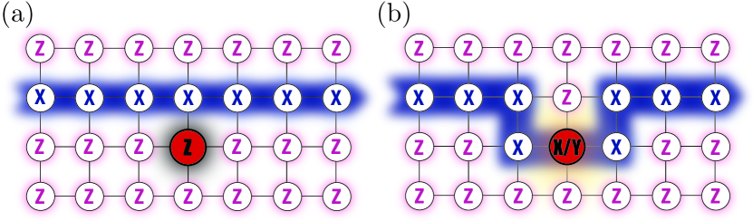
Figure 2: QCSI with modified cluster state $|{\Psi}\rangle$ and single-qubit $X_{i}$, $Y_{j}$, $Z_{k}$ Pauli measurements: the $Z$ measurements are used to cut out of the plane a web corresponding to some layout of a quantum circuit, while the $X$ measurements drive the MBQC simulation of this circuit Raussendorf and Briegel (2001). By “re-routing” a wire piece, one may choose between implementing and not implementing a non-Clifford gate. (a) Identity operation on the logical state space. (b) $X$ or $Y$ is measured adaptively to implement a logical $e^{-\textnormal{{i}}\text{{p}}/8\,Z}$ gate in MBQC Raussendorf and Briegel (2001).

Last, we present a family of magic states that promote our local QCSI scheme to universality. Unlike in standard magic state distillation Bravyi and Kitaev (2005), which relies on product magic states, our scheme has no entangling operations and requires entanglement to be present in the input to be universal. We show that a possibility is to use a modified cluster state $|{\Psi}\rangle$ that contains cells as in Fig. 2 with “red-site” qubits that are locally rotated by a $T$ gate $e^{-\textnormal{{i}}\text{{p}}/8\,Z}$. Our approach is to use such state to simulate a universal scheme of measurement based quantum computation based on adaptive local measurements $\{Z,X,Y,X\pm Y/\sqrt{2}\}$ on a regular 2D cluster state Raussendorf and Briegel (2001). Local Pauli measurements are available by assumption. Now, an on-site measurement of $X$ or $Y$ on one of the red qubits of $|{\Psi}\rangle$ has the same effect as measuring $(X\pm Y)/\sqrt{2}$ on a cluster state. To complete the simulation, it is enough to reroute the measurement-based computation through a red site (this can be done with the available $X$ measurements Raussendorf and Briegel (2001)) whenever a measurement of $(X\pm Y)/\sqrt{2}$ is needed. (See Fig. 2 for illustration.)

Note that an alternative resource state for one-qubit Pauli measurements is the so-called “union-jack” hypergraph state of Ref. Miller and Miyake (2016).

Conclusion.—In this Letter we investigated the role of contextuality in qubit QCSI and proved that it is a necessary resource for all such schemes that meet a simple minimal condition: namely, that the allowed measurements do not exhibit state-independent contextuality. Our result applies if and only if contextuality emerges as a physical property possessed by quantum states (with respect to the measurements available in the computational model). We extended earlier results on odd-prime dimensional qudits Veitch et al. (2012); Howard et al. (2014) and rebits Delfosse et al. (2015), and thereby completed establishing contextuality as a resource in QCSI in arbitrary prime dimensions. We conjecture that this result generalizes to all composite dimensions Gottesman (1998b) (the composite odd case was recently covered after completion of this work Delfosse et al. ) and to algebraic extensions of QCSI models based on normalizer gates Van den Nest (2013); Bermejo-Vega and Van Den Nest (2014); Bermejo-Vega et al. (2016, ); Bermejo-Vega and Zatloukal . Further, we demonstrated the applicability of our result to a concrete qubit QCSI scheme that does not exhibit state independent contextuality while retaining tomographic completeness.

Finally, we refer to a companion paper Raussendorf et al. (2017) where we investigate the role of Wigner functions in qubit QCSI. There, we use Wigner functions to motivate the near-classical sector of the free operations in qubit QCSI, and relate their Wigner-function negativity to contextuality and hardness of classical simulation. In comparison, in this Letter, constraint (C1) completely removes the need to introduce Wigner functions, and leads us to the simplest and most general proof that contextuality can be a resource in qubit QCSI that we are aware of. For this reason, we regard the establishing of condition (C1) as a fundamental structural insight of our Letter.

Acknowledgement.—We thank David T. Stephen and the anonymous reviewers for comments on the manuscript. JBV acknowledges financial support by by Horizon 2020 (640800-AQuS-H2020-FETPROACT-2014). ND is funded by Institute for Quantum Information and Matter (IQIM), the National Science Foundation Physics Frontiers Center (PHY-1125565) and the Gordon and Betty Moore Foundation (GBMF-2644). CO is supported by the Natural Sciences and Engineering Research Council of Canada (NSERC). RR is funded by NSERC and the Canadian Institute for Advanced Research (CIFAR). RR is scholar of the CIFAR Quantum Information Science program.

References

- Bravyi and Kitaev (2005) Sergey Bravyi and Alexei Kitaev, “Universal quantum computation with ideal Clifford gates and noisy ancillas,” Phys. Rev. A 71, 022316 (2005), quant-ph/0403025 .
- Gottesman (1997) Daniel Gottesman, Stabilizer Codes and Quantum Error Correction, Ph.D. thesis, California Institute of Technology (1997), quant-ph/9705052v1 .
- Gottesman (1998a) Daniel Gottesman, “Theory of fault-tolerant quantum computation,” Phys. Rev. A 57, 127–137 (1998a), quant-ph/9702029 .
- Veitch et al. (2012) Victor Veitch, Christopher Ferrie, David Gross, and Joseph Emerson, “Negative quasi-probability as a resource for quantum computation,” New J. Phys. 14, 113011 (2012), arXiv:1201.1256 .
- Howard et al. (2014) Mark Howard, Joel Wallman, Victor Veitch, and Joseph Emerson, “Contextuality supplies the ‘magic’ for quantum computation,” Nature 510, 351–355 (2014), arXiv:1401.4174 .
- Delfosse et al. (2015) Nicolas Delfosse, Philippe Allard Guerin, Jacob Bian, and Robert Raussendorf, “Wigner function negativity and contextuality in quantum computation on rebits,” Phys. Rev. X 5, 021003 (2015), arXiv:1409.5170 .
- Mermin (1990a) N. David Mermin, “Simple unified form for the major no-hidden-variables theorems,” Phys. Rev. Lett. 65, 3373–3376 (1990a).
- Peres (1990) Asher Peres, “Incompatible results of quantum measurements,” Phys. Lett. A 151, 107 – 108 (1990).
- Raussendorf et al. (2017) Robert Raussendorf, Dan E. Browne, Nicolas Delfosse, Cihan Okay, and Juan Bermejo-Vega, “Contextuality and Wigner-function negativity in qubit quantum computation,” Phys. Rev. A 95, 052334 (2017), arXiv:1511.08506 .
- Poulin (2005) D. Poulin, “Stabilizer formalism for operator quantum error correction,” Phys. Rev. Lett. 95, 230504 (2005), quant-ph/0508131 .
- Bermejo-Vega and Van Den Nest (2014) Juan Bermejo-Vega and Maarten Van Den Nest, “Classical simulations of Abelian-group normalizer circuits with intermediate measurements,” Quant. Info. Comput. 14, 181–216 (2014), arXiv:1210.3637 .
- Mermin (1990b) N. D. Mermin, “Extreme quantum entanglement in a superposition of macroscopically distinct states,” Phys. Rev. Lett. 65, 1838 (1990b).
- Raussendorf and Briegel (2001) Robert Raussendorf and Hans J. Briegel, “A one-way quantum computer,” Phys. Rev. Lett. 86, 5188–5191 (2001).
- Miller and Miyake (2016) Jacob Miller and Akimasa Miyake, “Hierarchy of universal entanglement in 2D measurement-based quantum computation,” npj Quantum Information 2, 16036 (2016), arXiv:1508.02695 .
- Gottesman (1998b) Daniel Gottesman, “Fault-tolerant quantum computation with higher-dimensional systems,” in Selected papers from the First NASA International Conference on Quantum Computing and Quantum Communications (Springer, New York, 1998) quant-ph/9802007 .
- (16) Nicolas Delfosse, Cihan Okay, Juan Bermejo-Vega, Dan E. Browne, and Robert Raussendorf, “Equivalence between contextuality and negativity of the Wigner function for qudits,” arXiv:1610.07093 .
- Van den Nest (2013) Maarten Van den Nest, “Efficient classical simulations of quantum Fourier transforms and normalizer circuits over abelian groups,” Quant. Inf. Comput. 13, 1007–1037 (2013), arXiv:1201.4867v1 .
- Bermejo-Vega et al. (2016) Juan Bermejo-Vega, Cedric Yen-Yu Lin, and Maarten Van den Nest, “Normalizer circuits and a Gottesman-Knill theorem for infinite-dimensional systems,” Quant. Inf. Comput. 16, 0361–0422 (2016), arXiv:1409.3208 .
- (19) Juan Bermejo-Vega, Cedric Yen-Yu Lin, and Maarten Van den Nest, “The computational power of normalizer circuits over black-box groups,” arXiv:1409.4800 .
- (20) Juan Bermejo-Vega and Kevin C. Zatloukal, “Abelian hypergroups and quantum computation,” arXiv:1509.05806 .