Ab initio Simulations of a Supernova Driven Galactic Dynamo in an Isolated Disk Galaxy

Abstract

We study the magnetic field evolution of an isolated spiral galaxy, using isolated Milky Way-mass galaxy formation simulations and a novel prescription for magnetohydrodynamic (MHD) supernova feedback. Our main result is that a galactic dynamo can be seeded and driven by supernova explosions, resulting in magnetic fields whose strength and morphology is consistent with observations. In our model, supernovae supply thermal energy, and a low level magnetic field along with their ejecta. The thermal expansion drives turbulence, which serves a dual role by efficiently mixing the magnetic field into the interstellar medium, and amplifying it by means of turbulent dynamo. The computational prescription for MHD supernova feedback has been implemented within the publicly available ENZO code, and is fully described in this paper. This improves upon ENZO’s existing modules for hydrodynamic feedback from stars and active galaxies. We find that the field attains $\mathrm{\mu G}$-levels over $\mathrm{Gyr}$-time scales throughout the disk. The field also develops large-scale structure, which appears to be correlated with the disk’s spiral arm density structure. We find that seeding of the galactic dynamo by supernova ejecta predicts a persistent correlation between gas metallicity and magnetic field strength. We also generate all-sky maps of the Faraday rotation measure from the simulation-predicted magnetic field, and present a direct comparison with observations.

1. Introduction

Magnetic fields exist throughout all types of galaxies. In spiral galaxies like our own, the fields typically attain several $\mathrm{\mu G}$ in strength, and exhibit long-range structure throughout the disk (see e.g. Beck, 2009, 2015, for recent reviews). The processes by which these fields have originated, and how they influence their host galaxy’s evolution remains the subject of intense observational and theoretical research. On the one hand, understanding the build-up of magnetic field by the galactic flow (the dynamo problem, see e.g. Moffatt, 1978; Parker, 1979) poses significant analytical and computational challenges. On the other, a galaxy’s magnetic field influences its pressure and flow profiles (Elstner et al., 2014), rate of star formation (Van Loo et al., 2014; Federrath & Klessen, 2012, 2013; Federrath, 2015), and cosmic ray transport processes (e.g. Strong et al., 2007). The co-evolution of galaxies and their magnetic fields is thus a complex and deeply significant problem.

The history of our galaxy’s magnetic field certainly includes a type of dynamo process, which has enhanced a pre-existing “seed” magnetic field and now maintains it at near-equipartition levels. It has long been appreciated that if the dynamo’s exponential folding time is the galactic rotation period, then it must have been seeded around the time of the Milky Way’s formation at a level not less than $\sim 10^{-20}\,\mathrm{G}$ (Rees, 1987). This has motivated extensive consideration of early universe processes that might have magnetized the primordial plasma from which the galaxy formed. However, a more modern view is that seeding by means of astrophysical processes, such as battery mechanisms, kinetic instabilities, or stellar feedback, would be of greater consequence than a primordial seed field (e.g. Blackman, 1998; Rees, 2006). It is also appreciated now that dynamo action is expected to grow the magnetic field at the turbulent diffusion rate, which is significantly faster than the orbital shear (Kulsrud & Anderson, 1992).

In this paper we address the question of how the magnetic field in a disk galaxy like the Milky Way would have evolved under the influence of stellar feedback alone. Within this narrative, the first significant magnetic fields would have been generated by turbulent convection within the interiors of early stars, and then dispersed by their winds or supernova explosions. Such feedback would inject magnetized plasma into the interstellar medium (ISM), while simultaneously driving turbulence that acts to disperse and amplify the field. We are thus investigating whether stars might have served as the seed for, and also the engine of galactic dynamo action. Our main result will be that this scenario offers a compelling resolution to the mystery of galactic magnetism, as it turns out to predict a magnetic field whose strength and morphology are consistent with what is known about the Milky Way’s magnetic field.

Our results are based on simulations of an initially unmagnetized galactic disk, coupled with a realistic prescription for star formation and magnetohydrodynamic (MHD) supernova feedback. In this prescription, supernova events occur in proportion to star formation activity, and provide localized injections of thermal energy, metal-rich material, and a low level of toroidal magnetic field. This is in contrast to a number of earlier studies in which supernovae were assumed to function strictly as sources of energetic cosmic rays (Hanasz et al., 2009; Siejkowski et al., 2014; Kulpa-Dybeł et al., 2011, 2015). In this study, we will neglect the influence of cosmic rays, and focus on the role of turbulence driven by supernovae through their thermal feedback. The fact that we ignore the cosmic rays, and yet recover results that are broadly consistent with earlier studies, suggests that galactic magnetism is a robust phenomenon, arising in response to several processes independently.

This computational approach will allow us to flesh out a number of details that have yet to be addressed within the supernova-driven galactic dynamo scenario. First, we wish to understand whether seed fields that are supplied locally, in small volumes around supernovae, can be mixed efficiently throughout the disk. We anticipate that if this mixing is efficient, then the outcome of our simulations may not differ dramatically from earlier ones in which a low-level seed field was imposed uniformly on the initial data (Wang & Abel, 2009; Rieder & Teyssier, 2016). We will also examine how seeding of magnetic fields by metal-rich supernova ejecta might induce a persistent correlation between metallicity and magnetism in the ISM. This is a non-trivial question because metals and magnetic flux experience distinct types of advective transport (scalar versus vector). Finally, there is the question of whether a supernova-driven dynamo leads to the development of large-scale magnetic structure. All of these questions will be addressed in the present work.

There have been a good number of studies focused on other aspects of the supernova-driven galactic dynamo. It has been simulated in a localized setting, with and without the effects of orbital shear (Gressel et al., 2008a, b). Global simulations were carried out by Wang & Abel (2009), using ENZO to study the formation and evolution of an isolated galaxy, onto which a seed field of $10^{-9}\,\mathrm{G}$ was imposed as part of the initial data. While that paper provides valuable insight on galactic magnetic field amplification, it does not include molecular cooling, star formation, or supernova feedback. Xu et al. (2009) used magnetic AGN feedback in galaxy clusters to show that turbulence in the ICM can amplify magnetic fields to observed values. Schleicher et al. (2010) investigated magnetic field growth via the small-scale dynamo for Kolmogorov and Burgers-type turbulence during the formation of the first stars and galaxies. Dubois & Teyssier (2010) introduced a more efficient method of including thermal supernova feedback in cosmological simulations using RAMSES and showed that dwarf galaxies seeded by magnetized supernova bubbles can attain magnetic fields of $\mu$G strength in 1 Gyr. (Teyssier, 2002) and studied its effect on the evolution of different types of galaxies. Beck et al. (2012) used the SPMHD code GADGET (Springel et al., 2001) to show that a primordial seed field can be amplified to equipartition strength in Milky-Way type galactic halos during virialization with the help of a small scale dynamo driven by supernova feedback. Pakmor & Springel (2013) observed exponential magnetic field amplification using an improved MHD implementation AREPO (Pakmor et al., 2011). However, instead of explicitly including thermal supernova feedback, they incorporated feedback with a modified equation of state. Rieder & Teyssier (2015) use RAMSES to build upon the work of Dubois & Teyssier (2010) and provide an in-depth study of the galactic amplification of a primordial magnetic field in the presence of thermal supernova feedback. Though they demonstrate that the turbulence created by supernova feedback drives the small-scale dynamo that amplifies the original magnetic field, they do not include magnetized supernova feedback.

Beck et al. (2013) incorporated magnetic seeding by supernova remnants in cosmological zoom-in simulations using GADGET. In their model, they inject a dipolar magnetic field in the range of $10^{-5}-10^{-3}\,\mathrm{G}$ into a volume of linear dimension 5 pc surrounding the supernova, which ultimately expands into a 25 pc radius bubble. The initial magnetic field is amplified to $\mathrm{\mu G}$ strengths through turbulent dynamo resulting from gravitational collapse, supernova feedback, and galactic mergers. They point out that even if a primordial magnetic seed field were present, it would have been washed out by the stronger fields supplied by supernovae. The goals of Beck et al. (2013) differ from our own in that their analysis focuses on a protogalactic halo, before it develops into a disk. Here we will study an isolated galactic disk, and neglect its merger history. We also model our injected magnetic fields with a toroidal geometry instead of poloidal, although we do not anticipate this difference to be consequential. Finally, we note that the inclusion of cosmic rays in simulations of galaxy formation is quickly becoming feasible; algorithms that afford a self-consistent treatment of the cosmic ray fluid within cosmological MHD frameworks have been described in Salem et al. (2014); Pfrommer et al. (2016); Pakmor et al. (2016b, a). Our choice to explore the role of thermal, as opposed to cosmic ray feedback processes, is based on a wish to understand the minimal conditions from which galactic magnetic fields are expected to arise.

Our paper is organized as follows. In §2, we describe our prescription for stellar formation and feedback, devoting particular attention to the numerical details of the magnetic field source term associated with the MHD supernova feedback. In §3, we present the results of our simulations, including a resolution study, images depicting the evolved magnetic field morphology, time series of the galactic magnetic energy budget, the power spectral distribution of magnetic energy, and correlation of magnetic field strength with gas density and metallicity. In §3.6 we present all-sky maps of the Faraday rotation measure generated from simulation data. Our findings are summarized in §5. There, we also draw comparisons with other numerical studies, speculate as to the mechanism by which our simulated galaxy develops its long-range magnetic field, and offer some reflection on the appearance of the earliest galactic magnetic fields.

Figure 1.— Two-dimensional schematic overview of the life cycle of a star cluster particle and two channels of its feedback. Left: Star cluster particle formation for an 80 pc resolution run (g80; see §2.2). Middle: Thermal feedback (see §2.3). Thermal energy by Type II supernova explosion is injected into the gas cell in which a star cluster particle of age less than 120 Myr resides . Right: Magnetic feedback (see §2.4). Toroidal magnetic fields are seeded within three finest cells from a star cluster particle.

2. Numerical Methods

2.1. Refinement, Hydrodynamics, and Radiative Cooling

We conduct this study by simulating isolated disk galaxies at three different resolutions using ENZO, a multi-physics cosmological magnetohydrodynamic (MHD) code that uses adaptive mesh refinement technology (AMR; Collins et al., 2010; Bryan et al., 2014). ENZO includes a wide range of relevant physics previously considered in galaxy-scale simulations (e.g. Kim et al., 2011, 2013a, 2013b) some of which are described in detail below.

The AMR function allows us to achieve higher resolutions more efficiently by only fully resolving areas of interest, designated by baryon and particle overdensities. Effectively, the entirety of our galactic disks were resolved at the highest level, while the outer edges of the simulation were able to remain less resolved to conserve computing time. The mass thresholds above which a cell is refined by factors of two in each axis are $M_{\rm ref,gas}=2.15\times 10^{4}M_{\odot}$ and $M_{\rm ref,part}=1.72\times 10^{6}M_{\odot}$ for gas and particles, respectively. In addition, the local Jeans length is always resolved by at least four cells to avoid artificial fragmentation (Truelove et al., 1997). We use a variety of grid configurations, ranging from a $64^{3}$ initial grid for a simulation box of 1.31 Mpc with 6 levels of refinement, to a $128^{3}$ initial grid with 7 levels of refinement. A combination of these grid conditions allows us to simulate a galaxy (described in Table 1) with three different minimum grid sizes of 320, 160, and 80 pc.

Table 1Simulation Parameters

Run ID	Minimum grid size (pc)	Disk initial metallicity ($Z_{\odot}$)	Supernova magnetic feedback parameters
			$L$ (pc)	$r_{\rm cutoff}$ (pc)	$\tau$ (Myr)	$t_{\rm cutoff}$ (Myr)	$E_{\rm tot,\,B}$ (ergs)
g320	320	1.0	262	786	0.2	1	$3.3\times 10^{48}$
g160	160	1.0	131	393	0.1	0.5	$3.3\times 10^{48}$
g160LM	160	0.001	131	393	0.1	0.5	$3.3\times 10^{48}$
g160LR	160	1.0	262	786	0.1	0.5	$3.3\times 10^{48}$
g80	80	1.0	79	236	0.025	0.1	$3.3\times 10^{48}$
g80LR	80	1.0	262	786	0.1	0.5	$3.3\times 10^{48}$

In order to solve the fluid conservation equations, we use a hyperbolic divergence cleaning approach with the MHD method that is described in Dedner et al. (2002) and is extensively tested in ENZO by Wang & Abel (2009) with various set-ups including an idealized disk formation simulation. In the work presented here, time integration is carried out by the total variation diminishing (TVD) 2nd order Runge-Kutta (RK) scheme (Shu & Osher, 1988). Spatial reconstruction employs the piecewise linear method (PLM; van Leer, 1977), and the flux at cell interfaces is computed with the local Lax-Friedrichs Riemann solver (LLF; Kurganov & Tadmor, 2000). A maximum 30% of the Courant-Friedrichs-Lewy (CFL) timestep is used to advance any fluid element in the simulation (i.e. hydrodynamic CFL safety number of 0.3). For a detailed description and testing of the MHD machinery we adopt, including the Dedner formulation of MHD equations in ENZO, we refer interested readers to Wang et al. (2008), Wang & Abel (2009), and references therein.

In addition, the gas in the ISM of our galaxy cools radiatively. Our equilibrium cooling follows pre-computed tabulated cooling rates from the photoionization code Cloudy (Ferland et al., 2013) provided via the Grackle chemistry and cooling library (Bryan et al., 2014; Kim et al., 2014), that is plugged in to ENZO. The pre-computed look-up table includes metal cooling rates for solar abundances as a function of gas density and temperature. These metal cooling rates will be scaled linearly with the metallicity that is being traced as a passive scalar field throughout our simulations. Uniform photoelectric heating of $8.5\times 10^{-26}\,\,{\rm erg\,s^{-1}cm^{-3}}$ is also considered without self-shielding (Tasker & Bryan, 2008). We however do not include the photoionization heating by the metagalactic ultraviolet background radiation from quasars and galaxies, leaving it for future exploration of the galaxy formation parameter space.

2.2. Star Cluster Particle Formation

The prescription for star formation and supernova feedback follows the algorithm first described in Cen & Ostriker (1992) with minor modifications. The finest cell (at the maximum level of refinement) of size $\Delta\,x$ and gas density $\rho_{\rm gas}$ produces a star cluster particle of initial mass $M_{\rm SC}^{\rm init}=0.1\,\rho_{\rm gas}\Delta\,x^{3}$ if all of the conditions below are met:

• the gas density is over $3.0\times 10^{-26}\,\mathrm{g\,cm^{-3}}$,

• the gas flow is converging (velocity field has negative divergence),

• the cooling time $t_{\rm cool}$ is shorter than the gas dynamical time $t_{\rm dyn}$ of the cell,

• the cell mass is larger than the local Jeans mass (Jeans unstable), and

• the cell has enough mass to create a particle of at least $M_{\rm thres}=3.0\times 10^{5}\,M_{\odot}$.

There are some notable differences between these conditions for star formation, and those adopted by other studies that also utilized ENZO (e.g. Tasker & Bryan, 2008). First, the prefactor $\Delta t/t_{\rm dyn}$ in Equation 1 of Tasker & Bryan (2008) is removed in order not to leave any unresolved mass behind when a star cluster particle is formed. Second, we do not impose “stochastic star formation”. And third, once created, a star cluster particle supplies thermal feedback (detailed below) into its surroundings for a fixed period of $120\,\mathrm{Myr}$ (rather than $12\,t_{\rm dyn}$).

2.3. Supernova Feedback: Thermal Energy Injection

Of the initial mass of a star cluster particle deposited, $M_{\rm SC}^{\rm init}$, 75% is eventually locked up in the particle after 12 $t_{\rm dyn}$. The actual stellar mass, $M_{*}$, formed inside a star cluster particle is described as a function of particle age $t$ by

$$M_{*}(t) =0.75\,M_{\rm SC}^{\rm init}\int_{0}^{\bar{t}}{\bar{t}}\,^{\prime}e^{-{\bar{t}}\,^{\prime}}\,d{\bar{t}}\,^{\prime}$$ (1)

$$=0.75\,M_{\rm SC}^{\rm init}\left[1-(1+{\bar{t}})e^{-\bar{t}}\right]\,,$$ (2)

where ${\bar{t}}=t/t_{\rm dyn}$.

Note that the actual stellar mass formation peaks at one dynamical time of the birthplace gas cell, $t_{\rm dyn}$. The rest of the particle mass, 0.25 $M_{\rm MC}^{\rm init}$, gradually returns to the cell in which the particle resides, along with $10^{-5}$ of the rest mass energy of $M_{*}$ (see Figure 1). This models $10^{51}$ ergs of thermal energy per every 42 $M_{\odot}$ of actual stellar mass formed. It is equivalent of Type II supernova explosion’s energy input and is enough to replenish the energy loss in ISM due to radiative cooling. Therefore, for a star cluster particle of initial mass $M_{\rm SC}^{\rm init}=M_{\rm thres}=3\times 10^{5}\,M_{\odot}$ which eventually produces $M_{*}=2.25\times 10^{5}\,M_{\odot}$, its supernova feedback event injects a total thermal energy of $E_{\rm tot,\,th}=5.4\times 10^{54}$ ergs. As discussed in §2.4, we will consider the case where the injected thermal energy dominates the total supernova feedback energy budget (i.e. $E_{\rm tot,\,B}\ll E_{\rm tot,\,th}$ thus $E_{\rm tot}\simeq E_{\rm tot,\,th}$). The ejecta mass blown back into the gas phase of ISM is recycled in the next generation of star formation. 2% of the ejecta mass is considered to be metals.

2.4. Supernova Feedback: Magnetic Field Injection

Balancing numerical resolution and the computational feasibility of a simulation is one of the major challenges in large numerical calculations. For this reason, in this work we aim to build a prescription for the magnetic field injection by supernova remnants with a simple geometry that could accurately be resolved by as few grid cells as possible. We propose that the best approximation is to source a toroidal loop of magnetic field around a star cluster particle (of mass $\sim 3\times 10^{5}\,M_{\odot}$) that generates a supernova feedback event (see Figure 1 and §2.3).

The spatial and temporal evolution of the injected magnetic energy is chosen to be

$$\dot{U}_{B,\,{\rm source}}=\tau^{-1}\frac{B_{0}^{2}}{4\pi}\frac{R}{L}e^{-r^{2}/L^{2}}e^{-t/\tau}(1-e^{-t/\tau})$$ (3)

where $t$ is the star cluster particle age, $R$ is the cylindrical radius, $r$ is the spherical radius, and $L$ and $\tau$ are the characteristic distance and time scale of a supernova magnetic feedback event, respectively. The time profile in Equation 3 increases from zero at $t=0$ to its characteristic value $\sim B_{0}^{2}/\tau$ around $t\sim\tau$, and then declines exponentially to zero with decay constant $\tau$.

By integrating the magnetic energy of the source field over all space and time, we acquire the expression for the normalization factor $B_{0}$ as

$$B_{0}^{2}=\frac{64}{3}\frac{\sigma E_{\rm tot}}{V_{\mathrm{SN}}}\,,$$ (4)

where $E_{\rm tot}$ is the total energy injected by a supernova feedback event, $\sigma$ is the proportion of the magnetic energy of the supernova to the total energy of the supernova, and $V_{\mathrm{SN}}=\frac{4}{3}\pi L^{3}$ is the volume of the supernova magnetic feedback event. Equations 3 and 4, combined with the relation $\dot{U}_{B,\,{\rm source}}=\mathbf{B}\cdot\dot{\mathbf{B}}/4\pi$ and our assumption that injected magnetic field is toroidal (along the randomly oriented local azimuthal unit vector $\hat{\mathbf{e}}_{\phi}$ for each event), yield an expression for the source term of magnetic field,

$$\dot{\mathbf{B}}_{\rm source}=\tau^{-1}B_{0}\left(\frac{R}{L}\right)^{1/2}e^{-r^{2}/2L^{2}}e^{-t/\tau}\,\hat{\mathbf{e}}_{\phi}\,.$$

In the presented simulations, we consider the case where the injected thermal energy dominates the total supernova feedback energy budget, that is, $E_{\rm tot,\,B}\ll E_{\rm tot,\,th}$ thus $E_{\rm tot}\simeq E_{\rm tot,\,th}$. For each supernova feedback event, we choose to inject a total magnetic energy of $E_{\rm tot,\,B}=\sigma E_{\rm tot}=3.3\times 10^{48}\,\mathrm{erg}$, implying $\sigma=6.1\times 10^{-7}$ for a star cluster particle of initial mass $3\times 10^{5}\,M_{\odot}$ (see §2.3). In addition, we set the characteristic distance scale of the magnetic feedback to be comparable with the minimum grid size of each run. For our choices of characteristic scale parameters $L$ and $\tau$ for each run, we refer the readers to Table 1. Lastly, because of numerical consideration, a cutoff distance and time are imposed when implementing the aforementioned $\dot{U}_{B,\,{\rm source}}$ and $\dot{\mathbf{B}}_{\rm source}$ formulae. We fiducially choose to cut off the exponential functions at $r_{\rm cutoff}=3L$ and at $t_{\rm cutoff}=5\tau$. Since limited numerical resolution requires that $L$ be much larger than the scale of an actual supernova remnant, we choose $L$ to be as small as possible, while remaining smoothly resolved on the grid. In practice, we find that numerical consistency between the actual magnetic energy introduced, and the integral over space and time of Equation 3, is acceptable when the supernova event occupies a subset of the computational domain as small as $3^{3}$ grid cells (see Figure 1). In our resolution comparison runs, g80LR and g160LR, the injection stencil matches that of the least-resolved run, g320.

2.5. Initial Condition

Our simulated galaxies are evolved from one of the isolated disk galaxy initial conditions (ICs) identified by the AGORA Collaboration (Kim et al., 2014), which strives to compare a wide range of galaxy simulations by creating a standardized set of ICs and feedback models. While the details of the proposed AGORA ICs are presented in the aforementioned paper, we summarize the aspect of the isolated ICs that might be of interest to readers. Note that by adopting isolated galactic disk ICs, we choose to ignore the effect of major and minor mergers. Here we already make an implicit assumption that such inter-galactic-scale dynamical interactions are secondary in the buildup of the galactic magnetic field.

The AGORA isolated IC was initially generated with the Makedisk code and distributed to the community as ASCII files in three resolution options. For our study we adopted the low-resolution version. The disk has a total mass of $M_{\rm d}=4.297\times 10^{10}\,\,M_{\odot}$, 80% of which is in $10^{5}$ stellar particles, and the rest 20% ($=f_{\rm gas}$) is in a gaseous disk that follows an analytic exponential profile

$$\rho(r,\,z)=\rho_{0}\ e^{-r/r_{\rm d}}\ e^{-|z|/z_{\rm d}}$$

with scale length $r_{\rm d}=$ 3.432 kpc, scale height $z_{\rm d}=$ 343.2 pc, and $\rho_{0}=M_{\rm d}f_{\rm gas}/4\pi r_{\rm d}^{2}z_{\rm d}$. The disk has an initial temperature of $10^{4}$ K, and an initial metallicity of $Z_{\rm d,init}=1\,Z_{\odot}$ for the g320, g160, g160LR, g80, g80LR runs, and $10^{-3}\,Z_{\odot}$ for the g160LM run (see Table 1). The stellar bulge of $1.25\times 10^{4}$ particles follows the Hernquist density profile (Hernquist, 1990) with a bulge to disk mass ratio of 0.1. The dark matter halo has a mass of $M_{200}=1.074\times 10^{12}\,\,M_{\odot}$ in $10^{5}$ particles, and follows the Navarro-Frenk-White profile (NFW; Navarro et al., 1997) with concentration parameter $c=10$ and spin parameter $\lambda=0.04$. This system is embedded in hot ($10^{6}$ K) gaseous medium, uniform in density across the entire simulation box of $(1.31\,\,{\rm Mpc})^{3}$. However the sum of this halo gas mass is only equal to the disk stellar mass, with zero velocity and negligible metallicity ($10^{-6}\,Z_{\odot}$), so it has negligible effect in the disk’s evolution. This IC models typical structural properties and gas fraction that are characteristic of Milky Way-like galaxies at $z\sim 1$.

3. Results

Here we describe the results of a family of simulated disk galaxies, evolved using the MHD supernova feedback model and initial conditions described in §2. Our family of models is summarized in Table 1. It is parameterized around the mesh spacing (in parsecs) of the finest grid blocks (those on the galactic plane). For example, in the run g160, the smallest cells are 160 parsecs in size. The scale $L$ over which supernova feedback is active is chosen to be smaller with increasing resolution, such that $L$ is roughly 3 grid cells across in each model. The composition of the supernova ejecta is given a metallicity of $Z_{\odot}$, with the exception of an additional run, g160LM, for which the metallicity was chosen to be $10^{-3}Z_{\odot}$. This choice allows us to rule out the possible influence of chemistry dependent cooling on the magnetic field evolution.

3.1. Magnetic Field Morphology

Figure 2.— The edge-on (left) and face-on (right) projections of the magnetic field strength (top), density (center), and temperature (bottom) of galaxy g80LR at t = 2.1 Gyr in 30 kpc boxes. Magnetic field streamlines are plotted in black over the image of the magnetic field strength.

The magnetic field in our disk galaxy simulations is illustrated in Figure 2. Shown there are density-weighted projections of magnetic and thermodynamic variables, taken 2.1 Gyr into the simulation at the highest resolution (model g80LR), with the disk shown edge-on in the left column, and top-down in the right. At this time, saturation of the magnetic energy throughout the disk is complete (see §3.2). Images are zoomed into the central $35\,\mathrm{kpc}$ of the simulation. The top row shows that the magnetic field strength attains levels of several $\mathrm{\mu G}$ near the disk mid-plane, and within roughly $10\,\mathrm{kpc}$ of the galactic center. In that image, we have also plotted streamlines of the magnetic field (projected onto the disk plane) to provide an impression of its overall geometry. From the top-down image, one sees that the field throughout the disk is predominantly azimuthal, with the radial field component $B_{R}$ being significantly lower than $B_{\phi}$. We believe this indicates that differential rotation of the disk is active at sustaining the field strength around its saturated value. Prevalence of the azimuthal field is consistent with observations e.g. IC 342, where the magnetic pitch angle is inferred to be relatively small (Sokoloff et al., 1992). We also note that the azimuthal field in our simulations changes sign at several radii. Those reversals imply the presence of magnetic neutral lines, which have been observed in M81 (Krause et al., 1989). The density profile indicates higher-density spiral arms, which correspond to areas of lower temperature and higher magnetic field strength.

The left column of Figure 2 illustrates the field morphology projected onto the meridional plane. The relative isotropy of meridional streamlines indicates that vertical and radial magnetic field components are comparable to one another ($B_{z}\sim B_{R}$). It is also evident from the relative smoothness of streamlines that the field is tangled at a smaller scale in the vicinity of the disk mid-plane than in the halo. Finally, we see that the halo magnetic field is considerably weaker than the field around the mid-plane. These observations are consistent with the view that agitation of the gas by supernovae, together with differential rotation of the disk, cooperatively maintain the short wavelength, equipartition-level magnetic field.

In contrast, the field in the halo is seen to be longer wavelength, and sub-equipartition. The relatively large coherency scale could be due to inverse transfer effects known to accompany turbulent relaxation (Zrake, 2014; Brandenburg et al., 2015; Zrake & East, 2016), or to mild turbulent driving supplied by the supernova outflows emerging from the disk. We favor the latter explanation because the halo magnetic field strength is sub-equipartition with respect to the kinetic energy density of turbulence, in other words motions driven externally are super-Alfvénic, so relaxation effects are not expected to be dominant here. The relatively large coherence scale of the halo magnetic fields is thus thought to arise from the presence of turbulent motions at a similar scale, which are in turn driven by the supernova outflows.

It is noteworthy that well-ordered poloidal magnetic field in galactic halos have been reported by e.g. Reuter et al. (1994), based on analysis of the $\mathrm{cm}$-wavelength synchrotron rotation measures of M82, and also by Dahlem et al. (1997), based on soft X-ray emission from high latitudes in NGC 4666. In both cases, the authors surmised the field regularity was due to inertial effects of a galactic wind. While that may be the case, the halo magnetic field in our simulated galaxies develops large-scale coherency even though no wind is driven from the galactic disk.

3.2. Magnetic Field Growth

Figure 3.— Top panel: The ratio of total magnetic energy of 40 kpc around the center of the galaxy to the total injected magnetic energy as a function of time. Middle panel: Proportion of the poloidal component of the magnetic field to the root-mean-square magnetic field value as a function of time. Bottom panel: The star formation rate as a function of time.

Figure 4.— The density weighted root-mean-square magnetic field strength as a function of time.

Our simulated disk galaxies are initialized in a completely unmagnetized state. The appearance of magnetic fields accompanies the first supernova explosions. Those fields are introduced at a very low level (only one part in $\sim 10^{8}$ of the supernova energy is in magnetic form). From there, enhancement of the magnetic field can only occur through some sort of dynamo action, which we define broadly as any conversion of kinetic into magnetic energy.

In the first phase of the magnetic field evolution, lasting roughly the first billion years, each of the galaxy models undergoes exponential growth of their total magnetic energy. In the top panel of Figure 3, we show the ratio total magnetic energy inside a $40\,\mathrm{kpc}$ sphere about the center of the domain to the total injected magnetic energy from supernova events, as a function of time. We note that in the first 500 million years, the total magnetic energy injected by the supernovae is higher than the total magnetic energy of the galaxy. This reflects that fact that magnetic energy may be reduced by adiabatic expansion or lost due to numerical dissipation, while net growth of the energy only occurs if dynamo action overwhelms those processes. We speculate that very early in the simulation, enhancement is weak because only the gas immediately nearby the supernova feedback sites is magnetized. As the magnetized gas is dispersed by turbulent mixing, amplification can occur rather uniformly throughout the disk. We believe that net enhancement (exponential growth) of magnetic energy commences once this initial mixing stage is complete. The exponential growth of the magnetic field does not follow a single straight-line (in log space) path, but can rather be divided into several stages of varying exponential growth rates. Model g320 reaches saturation at 1.5 Gyr, while the other three models reach saturation after only 1 Gyr.

We believe that exponential growth of the magnetic energy is best explained by operation of a small-scale turbulent dynamo. This process (also known as Kraichnan-Kazenstev dynamo (Kraichnan, 1968; Kazantsev, 1968), see also Brandenburg & Subramanian (2005); Tobias et al. (2011) for a review) describes enhancement of a vector field by advection and diffusion in a turbulent medium. Frozen-in advective transport of a vector field by a chaotic flow generally enhances lengths along the field lines exponentially in time. When that stretching effect prevails over resistive diffusion, exponential growth of the magnetic energy occurs. The time constant corresponds to the eddy turnover of the inner turbulence scale. Thus, the process runs to completion in a very short time, which only gets shorter as the Reynolds number increases. The process yields a spectral distribution of magnetic energy $P_{B}(k)$ that increases as $k^{3/2}$ up to the resistive cutoff scale. That is, when the magnetic Prandtl number is high (as it is in the interstellar medium), the early-stage magnetic energy is concentrated below the viscous cutoff scale. In our simulations, the magnetic Prandtl number ranges from $P_{m}\simeq 1$ in the cold, dense star forming regions to $P_{m}\simeq 10^{25}$ near the outskirts of the galactic disk, while the typical $P_{m}$ for the ambient ISM is around $10^{13}$. Once the small-scale magnetic energy density becomes comparable to the small-scale turbulent kinetic energy density, the Lorentz force begins to modify the turbulence in order to minimize further field line stretching, and the process enters a non-linear stage. Local simulations of the non-linear small-scale turbulent dynamo indicate that the magnetic energy attains scale-by-scale equipartition with the kinetic energy after a few turnovers of the largest eddies (Beresnyak, 2012; Zrake & MacFadyen, 2013; Schober et al., 2015). In the case of a disk galaxy, the small-scale dynamo completion time $\tau_{\rm dyn}$ is then $\sim h_{\rm disk}/v_{\rm eddy}$ where $h_{\rm disk}$ is the disk scale height and $v_{\rm eddy}$ is the RMS velocity of the eddies at scale $h_{\rm disk}$.

The second panel of Figure 3 adds yet another piece of evidence for the small-scale dynamo explanation. Here we plot how the strength of the poloidal component of the magnetic field as a fraction of the root-mean-square magnetic field strength varies with time. The poloidal component of the magnetic field oscillates in strength, and we do not observe the exponential growth that is predicted for large scale dynamo action. We note that although the galactic magnetic field is dominated by its toroidal component, that strength is set by the sum of many small-scale, arbitrarily oriented toroidal field loops.

3.3. Influence of the Star Formation Rate

The third panel of Figure 3 shows the star formation rate as a function of time for each of the four models. It provides a valuable complement to the first panel of that figure by informing us that the majority of star formation took place within the first billion years of the galaxy’s formation. We note that the initial star formation rate of model g80LR is much higher than those of the less-resolved models. The cause of this is purely numerical. In g80LR, the highest resolved grid cell was unable to hold as much mass as those in the less-resolved runs, which greatly stunted star particle formation. To resolve this issue, we chose to make the minimum mass required for star particles to be $2.5\times 10^{5}M_{\odot}$. This correction led to g80LR having roughly twice as many stars as the g320 and g160LR. The star formation rate continues having an influence on the magnetic field strength and topology even after the field saturates. Bursts of star formation contribute to the formation of bumps in the total-to-injected magnetic energy ratio. High star formation is also correlated with peak strengths of the poloidal magnetic field component. It is likely that increased turbulence from additional supernovae temporarily augment the poloidal component of the magnetic field.

Figure 4 shows the density weighted root-mean-square value of the magnetic field as a function of time for all of the simulated model galaxies. All models saturate around 6 $\mu G$ with the notable exception of models g80 and g80LR. We believe that bursts of star formation after t = 2.0 Gyr in model g80LR (see third panel of Figure 3) and after t = 2.5 Gyr in model g80 provide the extra turbulence necessary to raise the magnetic field strength to roughly 15 $\mu G$. We observe that models with the same minimum resolution share the same slope in the exponential growth of the magnetic field. The magnetic field e-folding timescale ranges from 40 Myr to 215 Myr with different model resolutions. This corresponds to magnetic field growth rates of $\Gamma\simeq 1\Omega-6\Omega$ assuming a galactic rotational period of 250 Myr. The magnetic field of g80 doesn’t reach $nG$ strengths until 1.2 Gyr, which is late compared to the other models. This is due to numerical dissipation around the small injection site and has no effect on the slope of the growth rate or the final magnetic field strength.

Recent studies have shown that the Jeans length scale needs to be resolved by at least 30 cells in order to capture the effect of the turbulent dynamo (Federrath et al., 2011; Turk et al., 2012). The Jeans length is defined as

$$\lambda_{J}=\left(\frac{\pi c_{s}^{2}}{G\rho}\right)^{1/2},$$ (5)

where $c_{s}$ is the sound speed of the gas, G is the gravitational constant, and $\rho$ is the density of the gas. From Figure 2, we estimate that the typical Jeans length in the galactic disk ranges from $\sim 5$ pc for the cold molecular gas to $\sim 3$ kpc for the warm ionized medium. Only our best-resolved models (g80 and g80LR) meet the 30 cell resolution criterion ($30\times 80\mathrm{pc}=2.4$ kpc) in the warm phases of the ISM. Considering that the turbulent warm phase of the ISM covers a large fraction of the disk’s volume, we interpret that the magnetic field growth in models g80 and g80LR is driven by the turbulent dynamo.

3.4. Spectral Distribution of Magnetic and Kinetic Energy

Figure 5.— The time evolution of the magnetic energy power spectrum with evenly spaced time intervals from $t=300\,\mathrm{Myr}$ to $t=3\,\mathrm{Gyr}$ for galaxy model g80LR at time intervals of $300\,\mathrm{Myr}$. The dashed line shows the power spectrum of the kinetic energy at $t=3\,\mathrm{Gyr}$. The dotted lines provide visual references of the Kolmogorov and Kazantsev power laws. These labels correspond to power laws with those familiar indices, but the data used to create the curve is $kP_{B}(k)$, which is $\propto k^{a+1}$ where $a=3/2$ or $-5/3$.

In this section we present power spectra which indicate the scalewise distribution of magnetic and kinetic energy. We briefly describe the procedure by which the spectral diagnostics are obtained from simulation data, and then we present results illustrating their evolution over time. In particular, we discuss how the spectrum, and its time evolution provides evidence for the operation of small-scale turbulent dynamo.

Power spectra are taken of the magnetic and kinetic energy per unit mass, which are defined as

$$P_{B}(k_{i}) = \frac{1}{\Delta k_{i}}\sum_{k_{i}<|\mathbf{q}|<k_{i}+\Delta k_{i}}\mathbf{b}_{\mathbf{q}}\cdot\mathbf{b}^{*}_{\mathbf{q}}/2,$$ (6)

$$P_{K}(k_{i}) = \frac{1}{\Delta k_{i}}\sum_{k_{i}<|\mathbf{q}|<k_{i}+\Delta k_{i}}\mathbf{v}_{\mathbf{q}}\cdot\mathbf{v}^{*}_{\mathbf{q}}/2,$$

where $\mathbf{b}_{\mathbf{q}}$ and $\mathbf{v}_{\mathbf{q}}$ are the Fourier amplitudes of the Alfvén velocity $\mathbf{b}=\mathbf{B}/\sqrt{4\pi\rho}$ and flow velocity $\mathbf{v}$ respectively, at wavenumber $\mathbf{q}$. The sum is over all wavenumbers whose magnitude lies in the bin of width $\Delta k_{i}$ centered at $k_{i}$. Fourier amplitudes are obtained using Fast Fourier Transform (FFT) routines provided by the Numpy module for Python. Since the simulation is performed using AMR, solution data needs to be resampled onto a uniform rectilinear mesh before being passed to the FFT. This latter stage is accomplished using the YT package to isolate a uniform data cube centered on the galactic disk. The data cube is sampled at $512^{3}$ lattice points covering $(20.6\,\mathrm{kpc})^{3}$.

Figure 6.— The distribution of cell mass as a function of density and magnetic field strength (left panel) and metallicity and magnetic field strength (right panel). The galaxy model pictured is g160LM after 3 Gyr of evolution. The data was taken from a sphere with a radius of 20 kpc about the center.

Figure 5 shows the temporal evolution of the power spectrum of the magnetic field energy as a function of the wavenumber k of the model g80LR. The coloring of the solid lines denotes the time at which the power spectrum was taken, starting with the yellow line at 0.3 Gyr, and ending with the deep blue line at 3.0 Gyr in 0.3 Gyr increments. The dashed black line represents the power spectrum of the kinetic energy of g80LR after saturation, at 3.0 Gyr. The two dotted lines serve as visual aids for the Kazantsev ($P_{B}\propto k^{3/2}$) and Kolmogorov ($P_{K}\propto k^{-5/3}$) power laws. General consistency between the early time magnetic energy spectrum and the Kazantsev spectrum suggests the magnetic field is being amplified by small-scale turbulent dynamo action. The dashed line in Figure 5 shows the kinetic energy spectrum, which is consistent with the Kolmogorov spectrum. The peak of the magnetic spectrum at saturation ($k_{*}\simeq 4\times 10^{-2}$ kpc^-1 lies at approximately 10 times the forcing scale, $k_{L}$. Also note that the late-time magnetic energy spectrum indicates that the magnetic field is marginally dominant at the small scales, and marginally sub-dominant at the large scales. These features are all consistent with the completion of non-linear small-scale turbulent dynamo in the saturation regime for high magnetic Prandtl numbers (Schekochihin et al., 2004; Schober et al., 2012, 2015). However, the geometry of our thin-disk galaxies poses a challenge in finding truly isotropic properties of magnetic and kinetic turbulence. The growth of the magnetic power spectrum could also be influenced by an efficient small-scale injection of the magnetic field, which is transported to larger scales through shear and rotation. Without performing control runs, our interpretation of the role of a turbulent small-scale dynamo remains speculative.

3.5. Metallicity-Magnetic Field Correlations

The left side of Figure 6 shows a 2D histogram of samples of the density and magnetic field strength throughout the disk. Each data point is also given a color corresponding to the cell mass at the sample location. In the right panel, the same samples are scattered according to their field strength and metallicity value, and colored according to the mass in a given cell. Data is shown from the low metallicity model, g160LM, after it was evolved for 1 Gyr. We choose g160LM because of its low initial metallicity, which makes it an excellent candidate to trace the contribution of metals from supernova events. At 1 Gyr, the magnetic field strength is attaining its saturated value (the time series data for g160LM is essentially the same as for g160, shown in Figure 3). The left panel reveals that the magnetic field is strongest in the dense regions of the galaxy, where star formation is prevalent. Meanwhile, the field strength and metallicity are weakest in the less-dense regions of the galaxy, which are found in the outskirts of the galactic disk and in the outer halo. From the right panel, we see that the magnetic field strength correlates with higher metallicity values. Though we already know supernova ejecta to be our sources of metals, we note that the magnetic field and high metallicity remain spatially coupled, even after the supernova events have ended. We note that this effect depends on the mixing efficiency of the ISM which operates on sub-grid scales and is therefore difficult to simulate effectively. Nevertheless, this is a distinct prediction made by the SN seed field / SN-driven dynamo scenario we have simulated for this study; if the seed field had been supplied uniformly in the initial condition, no magnetic field strength-metallicity correlation would be anticipated.

3.6. All-sky Rotation Measure Map

Magnetic fields in simulated galaxies such as the one reported in this article could be compared with actual observed data. The most detailed such galaxy-scale magnetic field observation is of our Milky Way galaxy. In this section, we compare our simulation results with Milky Way’s magnetic fields by constructing an all-sky map of Faraday rotation measures.

When electromagnetic waves travel through a magnetized interstellar medium, their planes of polarization rotate, and the amount of rotation is dependent upon the intervening magnetic field. Rotation measure (RM), defined below, is proportional to the magnetic field strength parallel to the line of sight, and the density of thermal electrons.

$${\rm RM}=\frac{e^{3}}{2\pi m_{e}^{2}c^{4}}\int^{L}_{0}n_{e}(s)B_{\parallel}(s)ds$$ (7)

Here $n_{e}$ is the thermal electron number density, $m_{e}$ is the mass of an electron, $B_{\parallel}$ is the magnetic field parallel to the line of sight, and $s$ is the line segment along the line of sight. Below we start by describing how this RM is evaluated in each lines of sight and how the all-sky RM map is constructed for our simulated galaxies.

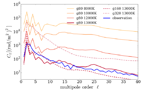
Figure 7.— Angular power spectra of the simulated all-sky Faraday rotation measure (RM) map. A series of yellow to red solid lines are for the g80LR run with varying ionization threshold temperatures $T_{\rm thres}=8000\,\mathrm{K}-13,000\,\mathrm{K}$ at $\sim 2.4\,\mathrm{Gyr}$. The blue solid line is for the Milky Way observation (Oppermann et al., 2012) whose corresponding all-sky map is reproduced in Figure 11. The dashed and dot-dashed lines are for g160LR and g320 runs, respectively, with $T_{\rm thres}=13,000\,\mathrm{K}$. The all-sky maps corresponding to g320, g160LR, g80LR runs with $T_{\rm thres}=13,000\,\mathrm{K}$ are Figures 8, 9, and 10 respectively.

In order to calculate RM, one first needs to estimate the number density of thermal electrons. Since we do not explicitly trace electron species in our simulations but only follow total gas density $\rho_{\rm gas}$, we choose to use the specific thermal energy of gas (per unit mass), $E_{\rm th}$, to estimate the ionization fraction $\chi(E_{\rm th})$ of hydrogen atoms, and then the thermal electron density $n_{e}$ in each cell as

$$n_{e}=\frac{\rho_{\rm gas}\chi(E_{\rm th})}{m_{\rm H}}$$ (8)

where $m_{\rm H}$ is the mass of a hydrogen atom.

If we assume that hydrogen becomes instantaneously fully ionized at temperature $T=T_{\rm thres}$, one can show that the ionization fraction is related to $E_{\rm th}$ as

$$\chi(\mu_{\rm eff}(E_{\rm th}))=\left\{\begin{array}[]{lr}0&\text{for }\mu_{\rm eff}\geq\mu_{\rm max}\\ \frac{4}{3\mu_{\rm eff}}-\frac{13}{12}&\text{for }\mu_{\rm min}\leq\mu_{\rm eff}\leq\mu_{\rm max}\\ 1&\text{for }\mu_{\rm eff}\leq\mu_{\rm min}\end{array}\right.$$ (12)

with an effective mean molecular weight function defined as

$$\mu_{\rm eff}(E_{\rm th})=\frac{3}{2}\frac{N_{\rm A}k_{\rm B}T_{\rm thres}}{E_{\rm th}},$$ (13)

where $N_{\rm A}$ is the Avogadro number, and $k_{\rm B}$ the Boltzmann constant. Here, if all hydrogen atoms are neutral, the mean molecular weight is $\mu_{\rm max}\simeq 1/(0.25/4+0.75/1)=1.23$, whereas if all hydrogen atoms are ionized, the mean molecular weight is $\mu_{\rm min}\simeq 1/(0.25/4+0.75/1\times 2)=0.64$. Note that the only free parameter in our formulation Eq.(12) is $T_{\rm thres}$, which should be $\sim 10^{4}\,{\rm K}$.

With Eqs.(8) to (13), one can evaluate the thermal electron density $n_{e}$ from the specific thermal energy $E_{\rm th}$. We then integrate $n_{e}(s)B_{\parallel}(s)$ along the line of sight as in Eq.(7) to acquire the rotation measure, then to produce an all-sky map like Figures 8 to 10. But first, in Figure 7, we plot the angular power spectra of all-sky RM maps for the g80LR run with 4 different ionization threshold temperatures ranging $T_{\rm thres}=8000\,{\rm K}$ to $13,000\,\mathrm{K}$ (yellow to red solid lines), in order to demonstrate how sensitive an RM map is to our choice of $T_{\rm thres}$. This figure is for $t\sim 2.4\,\mathrm{Gyr}$, well after galactic magnetic fields have reached nominal equilibrium values (see Figure 3). RM is proportional to thermal electron density, and we find that RM is highly sensitive to our understanding of how gas is ionized which is only crudely parametrized by $T_{\rm thres}$ in our model, Eq.(12). This illustrates the need to carefully characterize the ionization states of intervening medium to correctly understand the galactic magnetic field, which however is beyond the scope of this study. For the purpose of the current article, we opt to simply utilize the fact that $T_{\rm thres}=13,000\,\mathrm{K}$ best matches the observed Milky Way power spectrum assembled by Oppermann et al. (2012), shown here as a blue solid line. Therefore, we adopt $T_{\rm thres}=13,000\,\mathrm{K}$ for subsequent figures and discussion hereafter. Also in Figure 7, the power spectra for g160LR and g320 runs are plotted for comparison with $T_{\rm thres}=13,000\,\mathrm{K}$.

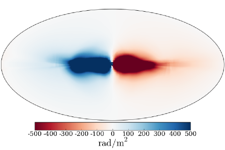
Figure 8.— All-sky RM map for the g320 run at $\sim 2.4\,{\rm Gyr}$ with $T_{\rm thres}=13,000\,\mathrm{K}$ and an origin 8 kpc away from the center of the galaxy. The angular power spectrum of this map is shown in Figure 7.

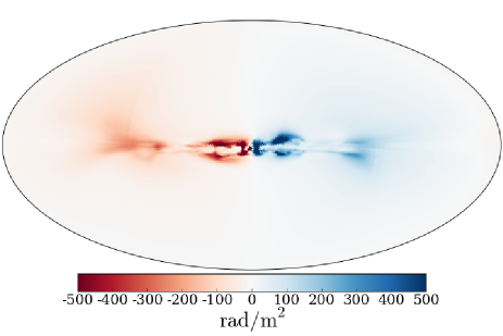
Figure 9.— All-sky RM map for the g160LR run at $\sim 2.4\,{\rm Gyr}$ with $T_{\rm thres}=13,000\,\mathrm{K}$ and an origin 8 kpc away from the center of the galaxy. The angular power spectrum of this map is shown in Figure 7.

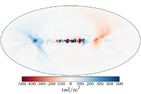
Figure 10.— All-sky RM map for the g80LR run at $\sim 2.4\,{\rm Gyr}$ with $T_{\rm thres}=13,000\,\mathrm{K}$ and an origin 8 kpc away from the center of the galaxy. The angular power spectrum of this map is shown in Figure 7.

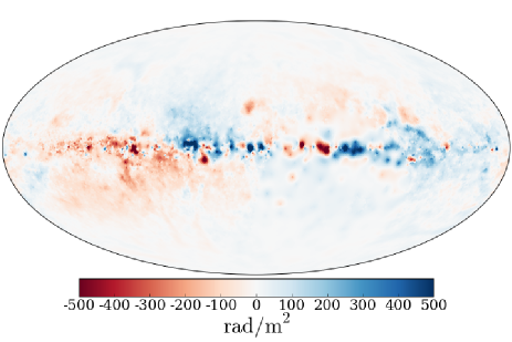
Figure 11.— All-sky RM map for the Milky Way galaxy, recreated from Oppermann et al. (2012). The angular power spectrum of this map is shown in Figure 7.

To construct simulated all-sky RM maps that mimic Oppermann et al. (2012), we position an observer at an approximate location of the Sun in our Milky Way: on the galactic disk plane about 8 kpc away from the Galactic Center. For this purpose, we first identify the location of highest density peak, $(x_{*},\,y_{*},\,z_{*})$, and define $z=z_{*}$ as the galactic disk plane. The origin (center) of the RM maps is then set on this plane, approximately 8 kpc from the galactic center in $x$-axis. By employing the Healpix pixelisation scheme (Górski et al., 2005), Figures 8 to 10 display the resulting all-sky RM maps at $\sim 2.4\,\mathrm{Gyr}$ for g320, g160LR and g80LR runs, respectively, with the ionization threshold temperature $T_{\rm thres}=13,000\,\mathrm{K}$. All these maps have the same angular resolution (i.e. Healpix parameter $N_{\rm side}=128$) that matches the observed Milky Way map in Figure 11. This Figure 11 is recreated from Oppermann et al. (2012) for comparison, using the raw data publicly available at http://wwwmpa.mpa-garching.mpg.de/ift/faraday.

Readers should be cautioned that the our RM maps and the corresponding power spectra are made for one particular snapshot ($\sim 2.4\,{\rm Gyr}$) of a greatly idealized disk galaxy, centered at an almost arbitrary location ($\sim$ 8 kpc from the galactic center in $x$-axis). Yet, several similarities are already noticeable between simulated and observed maps, such as the prominent magnetic field structure in disks, the existence of coherent large-scale field directions, and numerous smaller-scale structures possibly associated with turbulent small-scale eddies. The resemblance is the strongest for the g80LR run that has the smallest spatial resolution in our simulation suite. In particular, for the g80LR run, the spectral distribution of power in the multipole $l$-space is remarkably similar to the observed RM map, — albeit with a tuned $T_{\rm thres}$ value —, as can be seen in the angular power spectra of Figure 7. The model deviates from observations in the outer galaxy, where there is a lack of RM signal, both in strength and structure. This can be the result of several different factors. The first possibility is that the resolution of the grid decreases away from the galactic disk, which would wash out small-scale structure. The second is that the strength of the magnetic field outside of the galaxy is very weak along the plane of the disk because the magnetic field is ejected primarily through jets along the axis normal to the face of the disk. Since our snapshot is taken after 2.4 Gyr, there may not have been enough time for the surrounding medium to gain enough magnetic strength. Finally, our approximation of the ionization fraction neglects photoionization processes which would lead us to underpredict the RM signal in hot, low-density regions. Despite a highly idealized set-up, we conclude that our simulations reproduce an RM map and power spectrum that are close in shape to Milky Way’s — especially for a run with the finest resolution available.

4. Discussion

4.1. Comparison With Other Computational Approaches

Our approach is similar in certain ways to that taken by other groups. Hanasz et al. (2009) have also performed global disk galaxy simulations with magnetic fields introduced by supernovae. Whereas we used a toroidal magnetic configuration for the magnetic source term, they used randomly oriented magnetic dipoles. Their focus was on the role of cosmic rays in driving the galactic dynamo, so instead of introducing thermal energy as we did in our feedback prescription, they included a cosmic ray fluid that is sourced in the vicinity of supernova explosions. In their approach, only 10% of supernova events included a magnetic field. The same approach was adopted in Kulpa-Dybeł et al. (2011, 2015) to simulate dynamo activity in barred spiral galaxies, and by Siejkowski et al. (2014) to study dwarf galaxies. Beck et al. (2013) also utilized a magnetic dipole configuration as supernova source terms. Their simulations were carried out using an MHD version of the smoothed particle hydrodynamics (SPH) code GADGET, and were focused on magnetic evolution in a protogalactic halo instead of a disk galaxy. Wang & Abel (2009); Rieder & Teyssier (2016) carried out global disk galaxy simulations of a dynamo driven by hydrodynamic stellar feedback. In those studies a large-scale magnetic field was imposed on the initial model, rather than being seeded by the supernovae themselves. All studies appear to be in agreement regarding the saturation time-scale for turbulent dynamo.

4.2. Large Scale Magnetic Field

Throughout the course of our simulations, the magnetic field develops long-range structure. This behavior is somewhat surprising, given that small-scale turbulent dynamo, which we believe to be the driving mechanism, is not known to excite magnetic field modes of longer wavelength than that of the energy-containing turbulent eddies ($\lesssim h_{\rm disk}$). This could suggests that something akin to a mean-field dynamo (e.g. $\alpha-\Omega$) may be in effect. To determine whether that is the case, one could, in principle, measure the velocity-vorticity correlation from the simulation data to see if it has sufficient amplitude to explain the strength of the long wavelength magnetic field. Such a diagnostic could be a computational test of the arguments developed by Kulsrud & Anderson (1992), who pointed out that mean-field dynamo (which is a linear theory) may be quenched by back-reaction of the field, even at amplitudes well below equipartition.

Nevertheless, there are other mechanisms that may be responsible for the large-scale magnetic field structure seen in our simulations. As we saw in Section §3.5, the field strength is correlated with gas density. This suggests that the field enhancements could simply be tied to the density structure of the disk, which itself contains a long-wavelength component arising from self-gravitating effects. Another possibility is that the long-range field is simply the result of relaxation in regions where star formation is less active. There are at least two facts to support this view. First, it has been established observationally that the magnetic field of star-forming galaxies is generally stronger and more scrambled than in late-type galaxies (Chyży et al., 2007). Secondly, the condition for magnetic fields to exhibit self-assembly (inverse energy transfer) during turbulent relaxation turns out to be weaker than was previously believed. Although the presence of net magnetic helicity is known to be sufficient for inverse transfer to occur during relaxation (Frisch et al., 1975; Alexakis et al., 2006), it is now understood that is not a necessary condition; magnetic coherency increases due to statistical merging of locally relaxed magnetic structures even in non-helical field configurations (Zrake, 2014; Brandenburg et al., 2015). Thus, the development of large-scale structure, at least within regions of the disk where turbulence is not actively driven, should be anticipated even if the net helicity is negligible; it is unnecessary to invoke possible mechanisms by which magnetic helicity may be expelled from the disk (e.g. Sur et al., 2007).

4.3. Appearance of the Earliest Galactic Magnetic Fields

In the scenario we have simulated here, magnetic fields are first introduced alongside the first supernovae, which in our simulation occur in a fully formed, yet unmagnetized Milky Way type disk galaxy. This is not historically accurate, since the first stars and supernovae occurred at a much earlier epoch. Thus, our study should be interpreted as a proof of principle, that active star formation maintains galactic magnetic fields around equipartition levels. Since that star formation begins at an epoch preceding the disk galaxy phase we simulated here, a realistic narrative is that the protogalaxies that accreted to form the Milky Way were probably magnetized according to their level of star formation, and so the galactic disk inherited its first magnetic field from its progenitors. If agitation by supernova feedback were to terminate, then the magnetic field would relax and dissipate over the same time scale (the disk scale-height eddy turnover time) as it was built up. So, the strength and morphology of the magnetic field we observe in the evolved disk galaxy is arguably insensitive to initial conditions; had we begun the simulation with a disk magnetized at equipartition, supernova feedback would be expected to maintain it.

4.4. Role of Cosmic Rays

Our simulations use a stellar feedback prescription in which thermal energy and (small amounts of) magnetic energy are supplied by supernova explosions, but cosmic rays (CR’s) are not included. Interest in the role of CR’s in driving a galactic dynamo goes back to Parker (1992), who pointed out that their buoyancy can lead to stretching of the field which enhances its long-wavelength component. Several numerical studies have now been conducted (Hanasz et al., 2009; Siejkowski et al., 2014; Kulpa-Dybeł et al., 2011, 2015) that include CR effects coupled with MHD cosmological simulation. Overall, the results are surprisingly similar to our own; magnetic fields reach equipartition levels over $\mathrm{Gyr}$-time scales. This raises the question of the relative importance of the two primary types of energy supplied by supernovae — turbulence driven by the thermal expansion of the remnants themselves, and energy released as CR’s — since either by itself appears to be sufficient.

5. Conclusion

The existence of galactic magnetic fields is a significant puzzle in astrophysics and cosmology. In this paper, we have shown how those fields could have reached their present-day strength and morphology by stellar feedback processes alone. Weakly magnetized plasma is introduced to the galactic medium by stellar winds and supernova explosions, and the magnetic field is subsequently amplified by turbulence, driven by those same outflows. We carried out simulations of an isolated Milky Way type disk galaxy, that was initiated in an unmagnetized state. The galaxy was then evolved through an epoch of star formation and associated magnetohydrodynamic (MHD) feedback. Our simulations were continued through $3\,\mathrm{Gyr}$, at which time $\mathrm{\mu G}$-level magnetic fields were seen throughout much of the disk. Analysis of the time series and power spectrum of the magnetic field supports a picture in which small-scale turbulent dynamo, with turbulence sustained by supernova feedback, is the primary means by which the field reaches dynamically relevant strengths. The presence of differential rotation keeps the field marginally dominated by its toroidal component. In the scenario we have studied here, magnetic fields are injected in metal-rich supernova ejecta. Our simulations predict that a correlation between magnetization and metallicity should persist throughout galaxy’s evolution, and we argue that correlation is a distinct signature of a galactic dynamo seeded by supernova feedback. Finally, we presented synthetic all-sky maps of the Faraday rotation measure, as it would appear from Earth’s location relative to the galactic center. The angular power spectrum is found to match well to observations when the plasma ionization threshold temperature is chosen to be $13,000\,\mathrm{K}$.

In this work, we have also described a novel computational technique for simulating MHD supernova feedback processes. The simulation initial data we used is publicly available as part of the AGORA project. The initial model was evolved using the MHD version of the ENZO cosmological framework. We used the stellar formation algorithms that exist in the public version of that code, but modified the feedback prescription to include a magnetic field source term. The source term is chosen to inject a small fraction of the supernova energy as toroidal magnetic field, oriented relative to a randomly chosen vertical axis for each supernova event. The amplification and distribution of magnetic field in the evolved disk galaxies was found to be insensitive to the chosen injection radius or the initial metallicity of the ambient medium. Instead, the saturated field strength appears to be controlled by the level of turbulence sustained by stellar feedback. We also examined the influence of the magnetic field injection footprint size. Since resolution fine enough to resolve $\sim\mathrm{pc}$-scale supernova remnants remains computationally prohibitive, we ran a family of models with increasing resolution, and decreasing footprint size, between $320\,\mathrm{pc}$ and $80\,\mathrm{pc}$. The footprint size appears not to influence the outcome, suggesting that our conclusions would not change significantly if the injection scale was somehow reduced to astrophysically realistic values.

5.1. Acknowledgements

The authors thank Romain Teyssier, Michael Rieder, Klaus Dolag, and the anonymous referee for their insightful comments. I.B. would like to thank Sam Skillman for his time and help with ENZO.This work was performed in part under DOE Contract DE-AC02-76SF00515 and support by the Kavli foundation. The simulations were run on the Bullet cluster at the SLAC National Accelerator Laboratory and the Sherlock cluster at Stanford University.

References

- Alexakis et al. (2006) Alexakis, A., Mininni, P. D., & Pouquet, A. 2006, The Astrophysical Journal, 640, 335
- Beck et al. (2013) Beck, A. M., Dolag, K., Lesch, H., & Kronberg, P. P. 2013, MNRAS, 435, 3575
- Beck et al. (2012) Beck, A. M., Lesch, H., Dolag, K., et al. 2012, MNRAS, 422, 2152
- Beck (2009) Beck, R. 2009, Astrophysics and Space Sciences Transactions, 5, 43
- Beck (2015) —. 2015, The Astronomy and Astrophysics Review, 24, 4
- Beresnyak (2012) Beresnyak, A. 2012, Phys Rev Lett, 108, 35002
- Blackman (1998) Blackman, E. G. 1998, The Astrophysical Journal, 496, L17
- Brandenburg et al. (2015) Brandenburg, A., Kahniashvili, T., & Tevzadze, A. G. 2015, Physical Review Letters, 114, 075001
- Brandenburg & Subramanian (2005) Brandenburg, A., & Subramanian, K. 2005, Phys. Rep., 417, 1
- Bryan et al. (2014) Bryan, G. L., Norman, M. L., O’Shea, B. W., et al. 2014, ApJS, 211, 19
- Cen & Ostriker (1992) Cen, R., & Ostriker, J. P. 1992, ApJ, 399, L113
- Cho & Yoo (2012) Cho, J., & Yoo, H. 2012, eprint arXiv, 1209, 6130
- Chyży et al. (2007) Chyży, K. T., Bomans, D. J., Krause, M., et al. 2007, Astronomy and Astrophysics, 462, 933
- Collins et al. (2010) Collins, D. C., Xu, H., Norman, M. L., Li, H., & Li, S. 2010, ApJS, 186, 308
- Dahlem et al. (1997) Dahlem, M., Petr, M. G., Lehnert, M. D., Heckman, T. M., & Ehle, M. 1997, Astronomy and Astrophysics, 320
- Dedner et al. (2002) Dedner, A., Kemm, F., Kröner, D., et al. 2002, Journal of Computational Physics, 175, 645
- Dubois & Teyssier (2010) Dubois, Y., & Teyssier, R. 2010, A&A, 523, A72
- Elstner et al. (2014) Elstner, D., Beck, R., & Gressel, O. 2014, Astronomy & Astrophysics, 568, A104
- Federrath (2015) Federrath, C. 2015, Monthly Notices of the Royal Astronomical Society, 450, 4035
- Federrath & Klessen (2012) Federrath, C., & Klessen, R. S. 2012, The Astrophysical Journal, 761, 156
- Federrath & Klessen (2013) —. 2013, The Astrophysical Journal, 763, 51
- Federrath et al. (2011) Federrath, C., Sur, S., Schleicher, D. R. G., Banerjee, R., & Klessen, R. S. 2011, ApJ, 731, 62
- Ferland et al. (2013) Ferland, G. J., Porter, R. L., van Hoof, P. A. M., et al. 2013, 49, 137
- Frisch et al. (1975) Frisch, U., Pouquet, A., Leorat, J., & Mazure, A. 1975, Journal of Fluid Mechanics, 68, 769
- Górski et al. (2005) Górski, K. M., Hivon, E., Banday, A. J., et al. 2005, ApJ, 622, 759
- Gressel et al. (2008a) Gressel, O., Elstner, D., Ziegler, U., & Rüdiger, G. 2008a, Astronomy and Astrophysics, 486, L35
- Gressel et al. (2008b) Gressel, O., Ziegler, U., Elstner, D., & Rüdiger, G. 2008b, Astronomische Nachrichten, 329, 619
- Hanasz et al. (2009) Hanasz, M., Wóltański, D., & Kowalik, K. 2009, The Astrophysical Journal, 706, L155
- Hernquist (1990) Hernquist, L. 1990, ApJ, 356, 359
- Kazantsev (1968) Kazantsev, A. P. 1968, Soviet Physics JETP, 26, 1031
- Kim et al. (2013a) Kim, J.-h., Krumholz, M. R., Wise, J. H., et al. 2013a, ApJ, 775, 109
- Kim et al. (2013b) —. 2013b, ApJ, 779, 8
- Kim et al. (2011) Kim, J.-h., Wise, J. H., Alvarez, M. A., & Abel, T. 2011, ApJ, 738, 54
- Kim et al. (2014) Kim, J.-h., Abel, T., Agertz, O., et al. 2014, ApJS, 210, 14
- Kraichnan (1968) Kraichnan, R. H. 1968, Physics of Fluids, 11
- Krause et al. (1989) Krause, M., Beck, R., & Hummel, E. 1989, Astronomy and Astrophysics, 217
- Kulpa-Dybeł et al. (2015) Kulpa-Dybeł, K., Nowak, N., Otmianowska-Mazur, K., et al. 2015, Astronomy & Astrophysics, 575, A93
- Kulpa-Dybeł et al. (2011) Kulpa-Dybeł, K., Otmianowska-Mazur, K., Kulesza-Żydzik, B., et al. 2011, The Astrophysical Journal, 733, L18
- Kulsrud & Anderson (1992) Kulsrud, R. M., & Anderson, S. W. 1992, Astrophysical Journal, 396, 606
- Kurganov & Tadmor (2000) Kurganov, A., & Tadmor, E. 2000, Journal of Computational Physics, 160, 241
- Moffatt (1978) Moffatt, H. K. 1978, Cambridge, England, Cambridge University Press, 1978. 353 p.
- Navarro et al. (1997) Navarro, J. F., Frenk, C. S., & White, S. D. M. 1997, ApJ, 490, 493
- Oppermann et al. (2012) Oppermann, N., Junklewitz, H., Robbers, G., et al. 2012, A&A, 542, A93
- Pakmor et al. (2011) Pakmor, R., Bauer, A., & Springel, V. 2011, MNRAS, 418, 1392
- Pakmor et al. (2016a) Pakmor, R., Pfrommer, C., Simpson, C. M., Kannan, R., & Springel, V. 2016a, 15
- Pakmor et al. (2016b) Pakmor, R., Pfrommer, C., Simpson, C. M., & Springel, V. 2016b, 6
- Pakmor & Springel (2013) Pakmor, R., & Springel, V. 2013, MNRAS, 432, 176
- Parker (1979) Parker, E. N. 1979, Oxford, Clarendon Press; New York, Oxford University Press, 1979, 858 p.
- Parker (1992) —. 1992, The Astrophysical Journal, 401, 137
- Pfrommer et al. (2016) Pfrommer, C., Pakmor, R., Schaal, K., Simpson, C. M., & Springel, V. 2016, 30
- Rees (1987) Rees, M. J. 1987, Royal Astronomical Society, 28, 197
- Rees (2006) —. 2006, Astronomische Nachrichten, 327, 395
- Reuter et al. (1994) Reuter, H. P., Klein, U., Lesch, H., Wielebinski, R., & Kronberg, P. P. 1994, Astronomy and Astrophysics, 282
- Rieder & Teyssier (2015) Rieder, M., & Teyssier, R. 2015, ArXiv e-prints, arXiv:1506.00849
- Rieder & Teyssier (2016) Rieder, M., & Teyssier, R. 2016, Monthly Notices of the Royal Astronomical Society, 457, 1722
- Salem et al. (2014) Salem, M., Bryan, G. L., & Hummels, C. 2014, The Astrophysical Journal, 797, L18
- Schekochihin et al. (2004) Schekochihin, A. A., Cowley, S. C., Taylor, S. F., et al. 2004, Physical Review Letters, 92, 084504
- Schleicher et al. (2010) Schleicher, D. R. G., Banerjee, R., Sur, S., et al. 2010, A&A, 522, A115
- Schober et al. (2012) Schober, J., Schleicher, D., Bovino, S., & Klessen, R. S. 2012, Phys. Rev. E, 86, 066412
- Schober et al. (2015) Schober, J., Schleicher, D. R. G., Federrath, C., Bovino, S., & Klessen, R. S. 2015, Physical Review E, 92, 023010
- Schober et al. (2015) Schober, J., Schleicher, D. R. G., Federrath, C., Bovino, S., & Klessen, R. S. 2015, Phys. Rev. E, 92, 023010
- Shu & Osher (1988) Shu, C.-W., & Osher, S. 1988, Journal of Computational Physics, 77, 439
- Siejkowski et al. (2014) Siejkowski, H., Otmianowska-Mazur, K., Soida, M., Bomans, D. J., & Hanasz, M. 2014, Astronomy & Astrophysics, Volume 562, id.A136, 6 pp., 562, arXiv:1401.5293
- Sokoloff et al. (1992) Sokoloff, D., Shukurov, A., & Krause, M. 1992, Astronomy and Astrophysics, 264
- Springel et al. (2001) Springel, V., Yoshida, N., & White, S. D. M. 2001, 6, 79
- Strong et al. (2007) Strong, A. W., Moskalenko, I. V., & Ptuskin, V. S. 2007, Annual Review of Nuclear and Particle Science, vol. 57, Issue 1, p.285-327, 57, 285
- Sur et al. (2007) Sur, S., Shukurov, A., & Subramanian, K. 2007, Monthly Notices of the Royal Astronomical Society, 377, 874
- Tasker & Bryan (2008) Tasker, E. J., & Bryan, G. L. 2008, ApJ, 673, 810
- Teyssier (2002) Teyssier, R. 2002, A&A, 385, 337
- Tobias et al. (2011) Tobias, S. M., Cattaneo, F., & Boldyrev, S. 2011, eprint arXiv, 1103, 3138
- Truelove et al. (1997) Truelove, J. K., Klein, R. I., McKee, C. F., et al. 1997, ApJ, 489, L179
- Turk et al. (2012) Turk, M. J., Oishi, J. S., Abel, T., & Bryan, G. L. 2012, ApJ, 745, 154
- van Leer (1977) van Leer, B. 1977, Journal of Computational Physics, 23, 276
- Van Loo et al. (2014) Van Loo, S., Tan, J. C., & Falle, S. A. E. G. 2014, The Astrophysical Journal, 800, 7
- Wang & Abel (2009) Wang, P., & Abel, T. 2009, The Astrophysical Journal, 696, 96
- Wang et al. (2008) Wang, P., Abel, T., & Zhang, W. 2008, ApJS, 176, 467
- Xu et al. (2009) Xu, H., Li, H., Collins, D. C., Li, S., & Norman, M. L. 2009, ApJ, 698, L14
- Zrake (2014) Zrake, J. 2014, The Astrophysical Journal, 794, L26
- Zrake & East (2016) Zrake, J., & East, W. E. 2016, The Astrophysical Journal, 817, 89
- Zrake & MacFadyen (2013) Zrake, J., & MacFadyen, A. I. 2013, The Astrophysical Journal, 769, L29