Confinement-Deconfinement transition in $SU(2)+$Higgs Theory

Abstract

We study the confinement-deconfinement transition in $SU(2)$ gauge theory in the presence of massless bosons using lattice Monte Carlo simulations. The nature of this transition depends on the temporal extent ($N_{\tau}$) of the Euclidean lattice. We find that the transition is a cross-over for $N_{\tau}=2,4$ and second order with $3D$ Ising universality class for $N_{\tau}=8$. Our results show that the second order transition is accompanied by realization of the $Z_{2}$ symmetry.

I Introduction

Gauge theories such as quantum chromodynamics (QCD), standard model(SM) etc. at finite temperatures are relevant for describing the phase transitions in the early Universe and in the relativistic heavy-ion collisions. The pure gauge parts of these theories undergo the confinement-deconfinement (CD) transition Kuti:1980gh ; McLerran:1980pk at high temperatures. The corresponding pure gauge Euclidean actions are invariant under a class of gauge transformations represented by the center $Z_{N}$ of the $SU(N)$ group. This $Z_{N}$ symmetry Svetitsky:1985ye ; Svetitsky:1982gs plays an important role in the CD transition. In many ways, the nature of the CD transition is found to be similar to the transition in spin systems with $Z_{N}$ symmetry. The $Z_{N}$ symmetry is spontaneously broken in the deconfined phase by a non-zero thermal expectation value of the Polyakov loop. This leads to $N$ degenerate phases in the deconfined state.

In the fundamental representation, the $Z_{N}$ symmetry is explicitly broken in the presence of the matter fields. The $Z_{N}$ group can act only on the gauge fields and its action on the matter fields spoils their necessary temporal boundary condition. This explicit breaking affects the nature of the CD transition and the thermodynamic behavior of the phases themselves. It weakens the CD transition and, in the deconfined phase, all but only one of the $N$ phases become meta-stable. The explicit breaking vanishes when the matter fields are infinitely heavy. So it is expected that the explicit $Z_{N}$ symmetry breaking is small for large dynamical masses of the matter fields. In the mean field approximation of QCD, the explicit symmetry breaking turns out to be an effective “uniform” external field acting on the Polyakov loop Green:1983sd when the fermion masses are large. The strength of the external field grows as the masses decrease. Non-perturbative studies find that the CD transition in $SU(2)$ gauge theory with dynamical fermions is a crossover Nakamura:1984uz ; Heller:1984eq ; Heller:1985wc ; Kogut:1985xd ; Kogut:1985un . For $SU(3)$ gauge theory, the CD transition becomes a weak first order transition for large fermion mass Polonyi:1984zt ; Hasenfratz:1983ce ; Gavai:1985nz ; Fukugita:1986rr ; Karsch:2001nf . These results are consistent with the findings of the mean field approximation. However, an extrapolation of this effective external field to the chiral limit fails to explain the nature of the CD transition and the Polyakov loop behavior. In this case, the nature of the CD transition turns out to be the same as the chiral transition Digal:2002wn ; Fukushima:2002ew . This suggests that, in the chiral limit, the effective external field is a fluctuating and non-uniform dynamical field instead of a fixed uniform field. The behaviour of the chiral transition and the chiral condensate are, however, well described by a uniform/static field in the chiral limit Pisarski:1983ms .

It is expected that the explicit breaking of $Z_{N}$ due to bosonic matter fields also depends on mass. Perturbative calculations show that the explicit symmetry breaking increases with decrease in mass in presence of fermionic matter fields Gross:1980br ; Weiss:1981ev . A straightforward extension of these 1-loop calculations for bosonic fields gives similar results. For the massless case, the explicit symmetry breaking for $N=2$ is so large that there are no meta-stable states in the deconfined phase. These calculations, however, are not reliable near the CD transition. Strong coupling studies of lattice non-abelian gauge theories coupled to the Higgs field with the fixed radial mode find that the CD transition behaves like a pure gauge CD transition even for some finite non-zero coupling between the gauge and Higgs fields Fradkin:1978dv . For heavy Higgs fields, non-perturbative calculations find that the temperature dependence of the Polyakov loop expectation value shows a critical behavior above the CD transition point, i.e $\left<L\right>\sim(T-T_{c})^{1\over 3}$ Damgaard:1986qe ; Damgaard:1986jg . Recent study of the $Z_{N}$ symmetry Biswal:2015rul shows, within the numerical errors, that the strength of the explicit symmetry breaking vanishes even for a large but finite Higgs mass. These results indicate clear deviations from those of perturbative calculations in presence of matter fields. It is not clear whether the conventional expectation that the transition becomes weaker with the mass of matter fields, which is observed in QCD, also holds in the case of $SU(N)+$Higgs. To address this issue, we study the CD transition in the presence of the Higgs with vanishing bare mass using non-perturbative Monte Carlo simulations. We also compare the non-perturbative and perturbative results away from CD transition. To simplify our study, we consider $N=2$ and vanishing Higgs quartic coupling.

From lattice simulations, it is known that the thermal average of the Polyakov loop Svetitsky:1985ye ; Weiss:1981ev has strong cut-off dependence. The Polyakov loop expectation value decreases with the number of temporal cites ($N_{\tau}$) of the Euclidean lattice. However, the nature of the pure gauge CD transition does not depend on $N_{\tau}$ Datta:1999np ; Kogut:1982rt . In the presence of massless Higgs, this transition is found to be dependent on $N_{\tau}$. In this study, we find that this transition is a cross-over for $N_{\tau}=2,4$ and second order for $N_{\tau}=8$. These results suggest that in the continuum limit the CD transition is second order. We also look at the distribution of the Polyakov loop values in the thermal ensemble. The distribution in the case of $N_{\tau}=8$ clearly exhibits the $Z_{2}$ symmetry, which also explains why the CD transition is second order. This is surprising as one would expect maximal symmetry breaking as is observed in perturbative calculations Gross:1980br ; Weiss:1981ev as well as in lattice QCD Karsch:2001nf ; Digal:2000ar . Coincidentally the realization of the $Z_{2}(Z_{N})$ symmetry occurs only when the system is in the Higgs symmetric phase. This suggests that the strength of the Higgs condensate may be playing the role of the effective external field for the CD transition. We think that this restoration of the $Z_{2}(Z_{N})$ symmetry for larger $N_{\tau}$ is not due to the trivial continuum limit of pure Higgs theories Callaway:1988ya since the interaction between the gauge and Higgs increases with $N_{\tau}$. We discuss the possible reasons of this realization of $Z_{2}$ (or $Z_{N}$) symmetry in the Higgs symmetric phase later in section IV.

The paper is organized as follows. In section II we describe the $Z_{N}$ symmetry in $SU(N)+$Higgs theory. In section III we describe our simulations and results for $N=2$. This is followed by conclusions in section IV.

II The $Z_{N}$ symmetry in the presence of fundamental Higgs fields

The finite temperature partition function for a $SU(N)$ gauge field, $A_{\mu}$, in the path-integral formulation is given by

$${\cal Z}=\int[DA]e^{-S_{G}},$$ (1)

with the following gauge action

$$S_{G}=\int_{V}d^{3}x\int_{0}^{\beta}d\tau{1\over 2}\left[Tr\left(F^{\mu\nu}F_{\mu\nu}\right)\right],F_{\mu\nu}=\partial_{\mu}A_{\nu}-\partial_{\nu}A_{\mu}+g[A_{\mu},A_{\nu}].$$ (2)

The gauge field for a given Euclidean component $\mu$ is a $N\times N$ matrix, $A_{\mu}=T^{a}A^{a}_{\mu}$, where $T^{a}$’s are the generators of the $SU(N)$ group. Here $\beta$ is the inverse of the temperature $T$. The path-integration is over all $A_{\mu}$’s which are periodic along the temporal direction $\tau$, i.e $A_{\mu}(\tau)=A_{\mu}(\tau+\beta)$. This periodicity allows the gauge transformations $U(\tau)$ to be non-periodic along the temporal direction, up to a factor $z\in Z_{N}$ as

$$U(\tau=0)=zU(\tau=\beta).$$ (3)

Though the action is invariant under such gauge transformations, the Polyakov loop

$$L(\vec{\bf x})={1\over N}{\rm{Tr}}\left[{\rm{P}}\left\{\exp{\left(-ig\int_{0}^{\beta}A_{0}d\tau\right)}\right\}\right],$$ (4)

transforms as $L\longrightarrow zL$. In the deconfined phase $L$ acquires non-zero expectation value which gives rise to the spontaneous breaking of $Z_{N}$ symmetry. As a consequence, there are $N$ degenerate states in the deconfined phase characterized by each element of $Z_{N}$.

The full Euclidean action in the presence of a bosonic Higgs field $\Phi$ is given by

$$S=S_{G}+\int_{V}d^{3}x\int_{0}^{\beta}d\tau\left[{1\over 2}|D_{\mu}\Phi|^{2}+{m^{2}\over 2}\Phi^{\dagger}\Phi+{\lambda\over 4!}(\Phi^{\dagger}\Phi)^{2}\right],~{}{\rm{\large{with}}}~{}D_{\mu}\Phi=\partial_{\mu}\Phi+igA_{\mu}\Phi.$$ (5)

Here $m$ is the mass of the $\Phi$ field and $\lambda$ is the Higgs self interaction coupling constant. In the partition function

$${\cal Z}=\int[DA][D\Phi]e^{-S},$$ (6)

the path-integration of $\Phi$ is over all $\Phi$ fields which are periodic in $\tau$, i.e $\Phi(\tau)=\Phi(\tau+\beta)$. Under the action of the above gauge transformations (Eq. (3)), the transformed field $\Phi^{\prime}=U\Phi$ will not be periodic in $\tau$. So the actions of these gauge transformations have to be restricted to the gauge fields. Consequently, the action will increase under such gauge transformations, i.e $S(A^{\prime},\Phi)>S(A,\Phi)$. It is obvious that the increase in the action will change if the $\Phi$ field is varied ($\Phi\to\Phi^{\prime}$, but $\Phi^{\prime}\neq U\Phi$ ) as the gauge fields are gauge transformed. For some $\Phi$ configurations, it is possible to find $\Phi^{\prime}$ such that $S(A^{\prime},\Phi^{\prime})=S(A,\Phi)$ Biswal:2015rul . If these $\Phi$ configurations dominate the partition function, then the $Z_{N}$ symmetry will be effectively realized. In the following, we describe the simulations of the CD transition for $N=2$ and $m=0=\lambda$ using the above partition function.

III Simulations of the Confinement-Deconfinement transition

In the Monte Carlo (MC) simulations, the Euclidean space is discretized into $N_{\tau}\times N_{s}^{3}$ discrete points. $N_{\tau}=1/(aT)$ and $N_{s}=(L/a)$ are the number of lattice points along the temporal and spatial directions, respectively. $a$ is the lattice spacing and $L$ is the spatial extent of the Euclidean space. Each point $n$ on the lattice is represented by a set of four integers, i.e $n=(n_{1},n_{2},n_{3},n_{4})$. The Higgs field $\Phi_{n}$ lives on the lattice site $n$. The gauge link $U_{\mu}=\exp(-iagA_{\mu})$, on the other hand, lives on the link connecting the point $n$ to its nearest neighbor along the positive $\mu-$direction. The action with these discretized field variables with appropriate scaling in terms of $a$ for $m=0=\lambda$ is given by Kajantie:1995kf ,

$$S=\beta\sum_{p}{\rm{Tr}}(1-{U_{p}+U^{\dagger}_{p}\over 2})-{1\over 8}\sum_{\mu,n}{\rm{Re}}\left[(\Phi^{\dagger}_{n+\mu}U_{n,\mu}\Phi_{n})\right]+{1\over 2}\sum_{n}\left(\Phi^{\dagger}_{n}\Phi_{n}\right).$$ (7)

In Eq. (7), the first term represents the pure gauge action. $U_{p}$ is the product of the gauge links going anti-clockwise on the $p-$th elementary square/plaquette on the lattice. The Polyakov loop at any spatial point $n$ is given by the path order product of links on the shortest temporal loop going through $n$. The gauge transformation (Eq. (3)) of the gauge fields is equivalent to multiplication of all the temporal links on a fixed $\tau$ slice by $z\in Z_{N}$. The second term represents the interaction of the gauge and Higgs fields. This term is not invariant under the gauge transformations (Eq. (3)) of the gauge fields while the $\Phi$ field configuration is kept fixed. As mentioned above, the $\Phi$ fields can not be transformed under non-periodic gauge transformations.

In the Monte Carlo simulations, a sequence of statistically independent configurations of ($\Phi_{n}$,$U_{\mu,n}$) are generated. This is achieved by repeatedly updating an arbitrary initial configuration using numerical methods which follow the Boltzmann probability factor $e^{-S}$ and principle of detailed balance among the configurations in the sequence.  To update the gauge fields, we first use the standard heat bath algorithm Creutz:1980zw ; Kennedy:1985nu , and then update Higgs fields using pseudo heat bath algorithm Bunk:1994xs . We then again update the gauge fields using $4$ over-relaxation steps Whitmer:1984he after which Higgs fields are updated again using pseudo heat bath algorithm. To reduce auto-correlation between successive configurations along the sequence (Monte Carlo history) we carry out $10$ cycles of this updating procedure between subsequent measurements.  For our simulations, we use the publicly available MILC code milc and modify it to accommodate the Higgs fields.

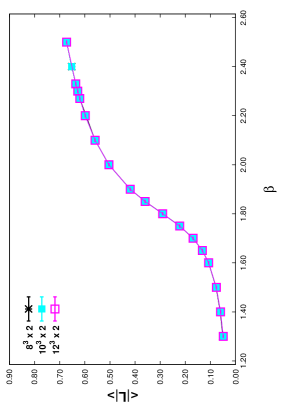
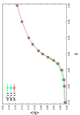
Figure 1: The Polyakov loop average $vs$ $\beta$ for (a) $N_{\tau}=2$, and (b) $N_{\tau}=4$.

The CD transition is studied for three values of $N_{\tau}=2$, we consider three spatial volumes, $N_{s}=8,10$ and $12$. For $N_{\tau}=4$ we consider $N_{s}=16,20$ and $24$ and for $N_{\tau}=8$, we consider $N_{s}=32,40$ and $48$. For each volume, we analyze $100,000$ configurations. However, we have lower statistics for $\beta$ values far away from $\beta_{c}$, particularly for the two biggest volumes $40^{3}\times 8$ and $48^{3}\times 8$. The Polyakov loop, susceptibility and Binder cumulant are computed for various values of $\beta$ to locate the transition point.

We carry out the error analysis using Jackknife method with a bin size of $10,000$ configurations. We also compute the volume average of $\Phi^{\dagger}\Phi$ and the interaction term. It is important to note that even though the $\Phi$ field is massless at the tree level, the fluctuations are finite. This is because the interaction with the gauge fields generate a non-zero finite mass for the $\Phi$ field. In the following section, we describe our simulation results.

III.1 The CD transition for $N_{\tau}=2$ and $4$

The Polyakov loop $\left<|L|\right>$ $vs$ $\beta$ for $N_{\tau}=2$ and $N_{\tau}=4$ are shown in Figs. 1 and 1, respectively. $\left<|L|\right>$ grows with $\beta$ with a sharp increase around the transition. The $1-\rm{loop}$ $\beta-$function temperature dependence of $\left<|L|\right>$ is found to be consistent with the power law, $\left<|L|\right>\sim(T-T_{c})^{1/3}$ Damgaard:1986jg . However $\left<|L|\right>$ does not show any volume dependence. The peak height of the Polyakov loop susceptibility does not vary with volume.

The Binder cumulant Binder:1981sa

$$U_{L}=1-{{\left<L^{4}\right>}\over{3\left<L^{2}\right>^{2}}},$$ (8)

for different $\beta$ are shown in Figs. 2 and 2 for $N_{\tau}=2$ and $N_{\tau}=4$, respectively. In both cases the variation in $U_{L}$ decreases for larger volume. For $N_{\tau}=2$, $U_{L}$ is almost flat against $\beta$. This behavior of the Binder cumulant is exactly the opposite of what is expected in a second order phase transition. The only explanation for these results is that the correlation length is finite and does not grow with volume. The sharp variation of the Polyakov loop around $\beta_{c}\sim 1.8\,(N_{\tau}=2)~{}\rm{and}~{}\beta_{c}\sim 2.29\,(N_{\tau}=4)$ only suggest a cross-over for the CD transition.

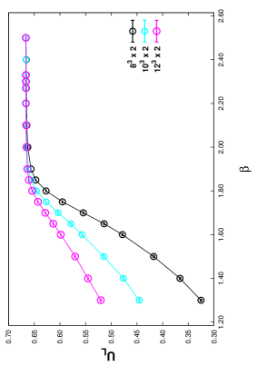
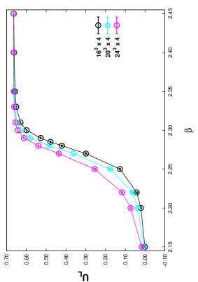
Figure 2: $U_{L}$ $vs$ $\beta$ for different volumes for (a) $N_{\tau}=2$, and (b) $N_{\tau}=4$.

III.2 The CD transition for $N_{\tau}=8$

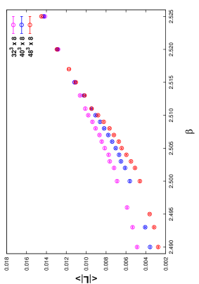
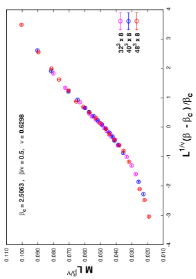
Figure 3: $N_{\tau}=8$. (a) The Polyakov loop $vs$ $\beta$ for different volumes, and (b) Scaled Polyakov loop $vs$ $\beta$ for different volumes.

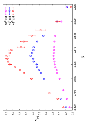
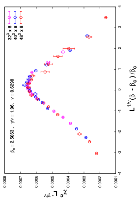
Figure 4: $N_{\tau}=8$. (a) Susceptibility $vs$ $\beta$ for different volumes, and (b) Scaled Susceptibility $vs$ $\beta$ for different volumes.

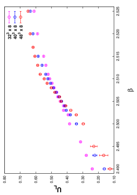
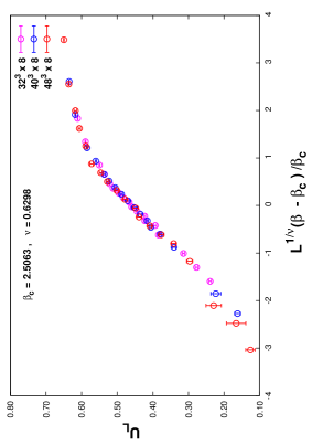
Figure 5: $N_{\tau}=8$. (a) The Binder cumulant $U_{L}$ $vs$ $\beta$ for different volumes, and (b) Scaled $U_{L}$ $vs$ $\beta$ for different volumes.

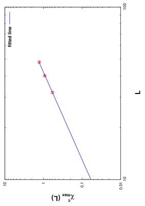
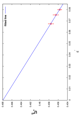
Figure 6: $N_{\tau}=8$. (a) The values of $\chi^{c}_{\mbox{\scriptsize max}}$ as a function of $L$ for $L=32,40$ and $48$. The slope of fitted line provides the value of $\gamma/\nu$. (b) The values of $U_{c}^{\rm{eff}}$ obtained from the crossing points of Binder Cumulant between two different volumes as a function of $\epsilon^{\prime}$. The intercept provides the value of $U_{c}$.

The behavior of the Polyakov loop for $N_{\tau}=8$ is completely different from that of $N_{\tau}=2$ and $4$. The Polyakov loop $\left<|L|\right>$ around the transition point $\beta_{c}$ behaves almost like the magnetization in the Ising model. The results for $\left<|L|\right>$ $vs$ $\beta$ for different volumes are shown in Fig. 3. In this case, $\left<|L|\right>$ clearly shows volume dependence. The volume dependence of the susceptibility $\chi^{c}$ of the Polyakov loop around the transition point is shown in Fig. 4. In Figs. 3 and 4, we show magnetization and susceptibility $vs$ $(L^{1/\nu}(\beta-\beta_{c})/\beta_{c})$, respectively. We see that both the quantitites collapse to single curves.

We find the value of the exponent, $\gamma/\nu$, by studying the finite size scaling (FSS) of the location of the maxima of the $\chi^{c}$’s similar to as in Kanaya:1994qe . However instead of using Rewieghting method to determine $\chi^{c}_{\mbox{\scriptsize max}}$, we use the Cubic Spline Interpolation method to generate a few hundred points close to ${\beta_{\chi}}_{\mbox{\scriptsize max}}$ for every Jackknife sample since we have reasonable amount of data near the peak for each volume. The scaling behavior of $\chi^{c}_{\mbox{\scriptsize max}}$ as a function of spatial volume, $L$, are shown in Fig. 6. We obtain $\gamma/\nu=1.98(2)$.

The Binder cumulant for $N_{\tau}=8$ is shown in Fig. 5. While the $U_{L}(\beta)$ for different volumes do not intersect for $N_{\tau}=2$ and $4$, they do for $N_{\tau}=8$ in a narrow region around the transition point. To determine $\beta_{c}$ and corresponding value of binder cumulant, we use the following finite size behavior of $U_{L}$ in the vicintiy of the critical point,

$$\displaystyle U_{L} \approx a_{0}+a_{1}\,(\beta-\beta_{c})/\beta_{c}\,L^{1/\nu}+a_{2}\,L^{-\omega}+\cdots.$$ (9)

By following the same procedure as in Fingberg:1992ju , we can write

$$\beta_{c}^{\rm{eff}} = \beta_{c}\,\left(1-\alpha\epsilon\right)\,,\,\,\,\mbox{where}\,\,\epsilon\,=\,L^{-1/\nu-\omega}\frac{1-b^{-\omega}}{b^{1/\nu}-1}\,\,,\,\,\,\,\,\,b\,=\,\frac{L^{\prime}}{L}\,,\,\,\,b>1.$$ (10)

The crossing point of the straight lines of two different spatial volumes provides $\beta_{c}^{\rm{eff}}$. By using the 3D Ising values of $\nu=0.6298$ and $\omega=0.825$, we obtain $\beta_{c}$ in the limit $\epsilon\rightarrow 0$ as $\beta_{c}=2.5064(4)$. Fig. 5 shows that $U_{L}$ $vs$ $(L^{1/\nu}(\beta-\beta_{c})/\beta_{c})$ for different volumes collapse to a single curve. To obtain infinite volume Binder Cumulant, $U_{c}$, we use the following relation

$$U_{c}^{\rm{eff}}=U_{c}\left(1+\alpha^{\prime}\epsilon^{\prime}\right)\,,\,\,\,\mbox{where}\,\,\epsilon^{\prime}\,=\,L^{-\omega}\frac{1-b^{-\omega-1/\nu}}{1-b^{-1/\nu}}$$ (11)

In Fig. 6, we show $U_{c}^{\rm{eff}}$ $vs$ $\epsilon^{\prime}$. In the limit $\epsilon^{\prime}\rightarrow 0$, we obtain $U_{c}=0.468(4)$. To determine the exponent $\beta/\nu$, we find magnetization at $\beta_{c}$ for each volume using Cubic Spline Interpolation. Using $\left.\langle|L|\rangle\right|_{\beta_{c}}\sim L^{\beta/\nu}$, we get $\beta/\nu=0.52(2)$.

The above values of $\beta/\nu$, ${\gamma/\nu}$ and $U_{L}(\beta_{c})$ from our computations are close to the $3D$ Ising values. These results seem to show that the CD transition transition for $N_{\tau}=8$ is a second order phase transition.

III.3 The $Z_{2}$ symmetry of the Polyakov loop

The different $N_{\tau}$ studies clearly show that the nature of the CD transition depends on $N_{\tau}$. The change in the nature of the CD transition from $N_{\tau}=8$ to $N_{\tau}=2,4$ is similar to that of the Ising transition when the external field is increased. So it is possible that the explicit breaking of the $Z_{2}$ symmetry decrease with increase in $N_{\tau}$. To check this, we compute the histogram of the Polyakov loop near the transition point for $N_{\tau}=2,4$ and $8$. For $N_{\tau}=2$ and $4$, no $Z_{2}$ symmetry is observed in the distribution of the Polyakov loop. On the deconfinement side and close to the transition point, the histograms always show one peak located on the positive real axis. Away from the transition point and inside the deconfinement phase, locally stable states are observed for which the Polyakov loop is negative. In Fig. 7 the histogram of the Polyakov loop $H(L)$ vs $|L|$ for $\beta=2.2$ is shown for $N_{\tau}=2$. $H(L)$ is normalized to $2$. There is no $Z_{2}$ symmetry either between the locations or the widths of the peaks. So the behavior of the Polyakov loop such as thermal average, fluctuations, correlation length etc. are found to be different for these two states. In contrast, the Polyakov loop exhibits $Z_{2}$ symmetry for $N_{\tau}=8$. Near the transition point, two peaks symmetrically located around $L=0$ on the real x-axis are observed. In Fig. 7, $H(L)$ $vs$ $|L|$ is shown for $\beta=3.20$. Though $10^{6}$ measurements are used to compute all the data points in Fig. 7, each individual point in the figure is the average over ($H(L)*10^{6}$) configurations for which the Polyakov loop values belong to a small bin centered at $L$. For example, the peaks of the histogram result from about $\sim 1.5\times 10^{4}$ configurations. It is interesting to see that $H(L)$ for $+L$ and $-L$ agree even with such small statistics. All physical observables which depend on the temporal gauge field such as gauge action and interaction term have same average when computed for the two $Z_{2}$ sector. These results suggest the effective realization of the $Z_{2}$ symmetry for $N_{\tau}=8$.

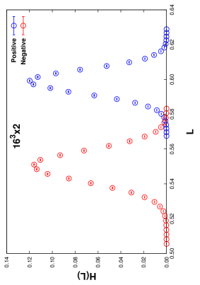
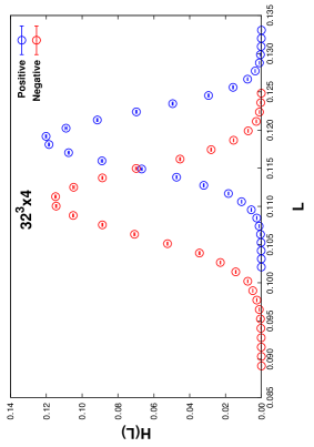
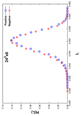
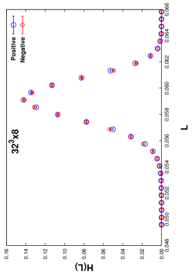
Figure 7: $H(L)\,vs\,|L|$. $H(L)$ is normalized to $2$. (a) $16^{3}\times 2$ lattice with $\beta=2.20$, (b) $32^{3}\times 4$ lattice with $\beta=2.35$, (c) $24^{3}\times 6$ lattice with $\beta=2.50$, and (d) $32^{3}\times 8$ lattice with $\beta=3.20$.

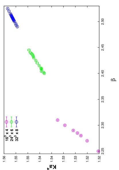
Figure 8: $Ka^{4}$ near $\beta_{c}$ for different $N_{\tau}$.

IV Discussions and Conclusions

In this work, we study the CD transition and $Z_{2}$ symmetry in $SU(2)+$Higgs theory for vanishing bare mass and quartic coupling of the Higgs field. We find that the cut-off effects are large. For $N_{\tau}=2$ and $4$, the CD transition turn out to be a crossover. The temperature dependence of the Polyakov loop average seems to show a critical behavior above the crossover point. However, no volume dependence is observed in any observable related to the Polyakov loop. For $N_{\tau}=8$, the temperature dependence, susceptibility and the Binder cumulant of the Polyakov loop show singular behavior suggesting a second order CD transition. Our results for the critical exponents are found to be consistent with the $3D$ Ising universality class.

The singular behavior of the Polyakov loop for $N_{\tau}=8$ is accompanied by the effective realization of the $Z_{2}$ symmetry. $Z_{2}$ symmetric peaks are observed in the histogram of the Polyakov loop in the deconfined phase near to the transition point. Thermal averages such as the fluctuations of the Polyakov loop, interaction term between the gauge and the Higgs field, the gauge action etc. are all found to be same for the two deconfined states related by $Z_{2}$ symmetry. Note that the interaction between the Higgs and gauge fields are non-zero which implies that the realization of the $Z_{2}$ symmetry is not due to the vanishing or small interaction. We observe that the interaction in a given physical volume increases with $N_{\tau}$. From $N_{\tau}=4$ to $6$ , the interaction increases by a factor of $\sim 5.12$ and , from $N_{\tau}=6$ to $8$ , it increases by a factor of $\sim 3.18$. In our simulations, we find that fluctuations of the Higgs field play an important role. $Z_{2}$ flip of the gauge fields are always accompanied by ”realignment” ($\Phi\to\Phi^{\prime}$) of the Higgs configuration. As soon as the Higgs fluctuations are frozen/fixed, the explicit breaking of $Z_{2}$ reappears. The reason why the $Z_{2}$ realization happens for $N_{\tau}=8$ and not for $N_{\tau}=2$ and $4$ is the increase in the phase space of $\Phi$ field with $N_{\tau}$. With the increase in the phase space, it is more likely that for a given $\Phi$ there exists a $\Phi^{\prime}$ which can compensate for the increase in action due to $Z_{2}$ rotation of the gauge fields. We find that the likelihood of finding such a $\Phi^{\prime}$ increases with $N_{\tau}$. It is important to note that the $Z_{2}$ symmetry in our simulations only implies that a $\Phi^{\prime}$ exists for every statistically significant $\Phi$. It is obvious that there will be $\Phi$ configurations for which there won’t be any $\Phi^{\prime}$ even in the limit $N_{\tau}\to\infty$. This is expected to happen when the Higgs field acquires a condensate. In this sense, the restoration/realization of the $Z_{2}$ symmetry is not exact, and the explicit symmetry breaking is not zero but statistically insignificant.

Our results may have important implications for the study of $Z_{N}$ symmetry in the presence of matter fields. Conventionally, it is expected that in the massless limit there will be maximal breaking of the $Z_{2}$ symmetry and the CD transition will be a crossover. $1$-loop perturbative calculations Gross:1980br ; Weiss:1981ev for fermions suggest that the explicit breaking for the massless case will be so large that there will be no meta-stable states in the entire deconfinement phase. A straightforward extension for bosonic fields gives similar results. However, our non-perturbative results suggest that the explicit breaking is so minimal that meta-stable states tend become degenerate with the stable state in the continuum. It would be interesting to see if similar realization of the $Z_{N}$ symmetry happens for different $N$ and also in the presence of fermion fields. We plan to study these issues in our future work.

Acknowledgements

All our numerical computations have been performed at Annapurna supercluster based at the Institute of Mathematical Sciences, India and HybriLIT supercluster based at Joint Institute for Nuclear Research, Dubna, Russia. We have used the MILC collaboration’s public lattice gauge theory code (version 6) milc as our base code.

REFERENCES

REFERENCES

- (1) J. Kuti, J. Polonyi and K. Szlachanyi, Phys. Lett. B 98, 199 (1981). doi:10.1016/0370-2693(81)90987-4
- (2) L. D. McLerran and B. Svetitsky, Phys. Lett. B 98, 195 (1981). doi:10.1016/0370-2693(81)90986-2
- (3) B. Svetitsky, Phys. Rept. 132, 1 (1986). doi:10.1016/0370-1573(86)90014-1
- (4) B. Svetitsky and L. G. Yaffe, Nucl. Phys. B 210, 423 (1982). doi:10.1016/0550-3213(82)90172-9
- (5) F. Green and F. Karsch, Nucl. Phys. B 238, 297 (1984). doi:10.1016/0550-3213(84)90452-8
- (6) A. Nakamura, Phys. Lett. 149B, 391 (1984). doi:10.1016/0370-2693(84)90430-1
- (7) U. M. Heller and F. Karsch, Nucl. Phys. B 258, 29 (1985). doi:10.1016/0550-3213(85)90601-7
- (8) U. M. Heller, Phys. Lett. 163B, 203 (1985). doi:10.1016/0370-2693(85)90221-7
- (9) J. B. Kogut, J. Polonyi, H. W. Wyld and D. K. Sinclair, Phys. Rev. D 31, 3307 (1985). doi:10.1103/PhysRevD.31.3307
- (10) J. B. Kogut, J. Polonyi, H. W. Wyld and D. K. Sinclair, Nucl. Phys. B 265, 293 (1986). doi:10.1016/0550-3213(86)90310-X
- (11) J. Polonyi, H. W. Wyld, J. B. Kogut, J. Shigemitsu and D. K. Sinclair, Phys. Rev. Lett. 53, 644 (1984). doi:10.1103/PhysRevLett.53.644
- (12) P. Hasenfratz, F. Karsch and I. O. Stamatescu, Phys. Lett. 133B, 221 (1983). doi:10.1016/0370-2693(83)90565-8
- (13) R. V. Gavai and F. Karsch, Nucl. Phys. B 261, 273 (1985). doi:10.1016/0550-3213(85)90575-9
- (14) M. Fukugita and A. Ukawa, Phys. Rev. Lett. 57, 503 (1986). doi:10.1103/PhysRevLett.57.503
- (15) F. Karsch, E. Laermann and C. Schmidt, Phys. Lett. B 520, 41 (2001) doi:10.1016/S0370-2693(01)01114-5 [hep-lat/0107020].
- (16) S. Digal, E. Laermann and H. Satz, Nucl. Phys. A 702, 159 (2002). doi:10.1016/S0375-9474(02)00700-5
- (17) K. Fukushima, Phys. Lett. B 553, 38 (2003) doi:10.1016/S0370-2693(02)03184-2 [hep-ph/0209311].
- (18) R. D. Pisarski and F. Wilczek, Phys. Rev. D 29, 338 (1984). doi:10.1103/PhysRevD.29.338
- (19) D. J. Gross, R. D. Pisarski and L. G. Yaffe, Rev. Mod. Phys. 53, 43 (1981). doi:10.1103/RevModPhys.53.43
- (20) N. Weiss, Phys. Rev. D 25, 2667 (1982). doi:10.1103/PhysRevD.25.2667
- (21) E. H. Fradkin and S. H. Shenker, Phys. Rev. D 19, 3682 (1979). doi:10.1103/PhysRevD.19.3682
- (22) P. H. Damgaard and U. M. Heller, Nucl. Phys. B 294, 253 (1987). doi:10.1016/0550-3213(87)90582-7
- (23) P. H. Damgaard and U. M. Heller, Phys. Lett. B 171, 442 (1986). doi:10.1016/0370-2693(86)91436-X
- (24) M. Biswal, S. Digal and P. S. Saumia, arXiv:1511.08295 [hep-lat].
- (25) S. Datta and R. V. Gavai, Phys. Rev. D 60, 034505 (1999) doi:10.1103/PhysRevD.60.034505 [hep-lat/9901006].
- (26) J. B. Kogut, M. Stone, H. W. Wyld, W. R. Gibbs, J. Shigemitsu, S. H. Shenker and D. K. Sinclair, Phys. Rev. Lett. 50, 393 (1983). doi:10.1103/PhysRevLett.50.393
- (27) S. Digal, E. Laermann and H. Satz, Eur. Phys. J. C 18, 583 (2001) doi:10.1007/s100520000538 [hep-ph/0007175].
- (28) D. J. E. Callaway, Phys. Rept. 167, 241 (1988). doi:10.1016/0370-1573(88)90008-7
- (29) K. Kajantie, M. Laine, K. Rummukainen and M. E. Shaposhnikov, Nucl. Phys. B 466, 189 (1996) doi:10.1016/0550-3213(96)00052-1 [hep-lat/9510020].
- (30) M. C reutz, Phys. Rev. D 21, 2308 (1980). doi:10.1103/PhysRevD.21.2308.
- (31) N. Cabibbo and E. Marinari, Phys. Lett. B 119, 387 (1982). doi:10.1016/0370-2693(82)90696-7.
- (32) A. D. Kennedy and B. J. Pendleton, Phys. Lett. 156B, 393 (1985). doi:10.1016/0370-2693(85)91632-6
- (33) B. Bunk, Nucl. Phys. Proc. Suppl. 42, 566 (1995). doi:10.1016/0920-5632(95)00313-X.
- (34) C. Whitmer, Phys. Rev. D 29, 306 (1984). doi:10.1103/PhysRevD.29.306.
- (35) http://www.physics.utah.edu/~detar/milc/.
- (36) K. Binder, Z. Phys. B 43, 119 (1981). doi:10.1007/BF01293604
- (37) K. Kanaya and S. Kaya, Phys. Rev. D 51, 2404 (1995) doi:10.1103/PhysRevD.51.2404 [hep-lat/9409001].
- (38) J. Fingberg, U. M. Heller and F. Karsch, Nucl. Phys. B 392, 493 (1993) doi:10.1016/0550-3213(93)90682-F [hep-lat/9208012].