The redshifted HI 21 cm signal from the post-reionization epoch: Cross-correlations with other cosmological probes

Abstract

Tomographic intensity mapping of the H i using the redshifted 21 cm observations opens up a new window towards our understanding of cosmological background evolution and structure formation. This is a key science goal of several upcoming radio telescopes including the Square Kilometer Array (SKA). In this article we focus on the post-reionization signal and investigate the of cross correlating the 21 cm signal with other tracers of the large scale structure. We consider the cross-correlation of the post-reionization 21 cm signal with the Lyman-$\alpha$ forest, Lyman-break galaxies and late time anisotropies in the CMBR maps like weak lensing and the Integrated Sachs Wolfe effect. We study the feasibility of detecting the signal and explore the possibility of obtaining constraints on cosmological models using it.

1 Introduction

The tomographic intensity mapping of the neutral hydrogen (H i ) distribution through redshifted HI 21-cm signal observation is an important probe of cosmological evolution and structure formation in the post reionization epoch (Bharadwaj & Sethi, 2001; Wyithe & Loeb, 2009; Loeb & Wyithe, 2008; Chang et al., 2008). The astrophysical processes dominating the epoch of reionization is now believed to have completed by redshift $z\sim 6$ (Fan et al., 2006). In the post-reionization era most of the neutral HI gas are housed in the Damped Ly-$\alpha$ (DLA) systems. These DLA clouds are the predominant source of the HI 21-cm signal. Intensity mapping involves a low resolution imaging of the diffuse HI 21-cm radiation background without attempting to resolve the individual DLAs. Such a tomographic imaging shall naturally provide astrophysical and cosmological data regarding the large scale matter distribution, structure formation and background cosmic history in the post-reionization epoch (Chang et al., 2008; Wyithe, 2008; Bharadwaj et al., 2009; Camera et al., 2013; Bull et al., 2015). Several functioning and upcoming radio interferometric arrays like Giant Metrewave Radio Telescope (GMRT) , the Ooty Wide Field Array (OWFA) (Ali & Bharadwaj, 2014), the Canadian Hydrogen Intensity Mapping Experiment (CHIME) , the Meer-Karoo Array Telescope (MeerKAT) , the Square Kilometer Array (SKA) are aimed towards detecting the cosmological 21-cm background radiation. Detecting the 21 cm signal, is however extremely challenging. This is primarily because of the large astrophysical foregrounds (Santos et al., 2005; Di Matteo et al., 2002; Ghosh et al., 2010) from galactic and extra-galactic sources which are several order of magnitude greater than the signal .

Cross-correlating the 21 cm signal with other probes may prove to be useful towards mitigating the severe effect of foreground contaminants and other systematic effects which plague the signal. The main advantage of cross-correlation is that the cosmological origin of the signal can only be ascertained only if it is detected with high a statistical significance in the cross- correlation. Cosmological parameter estimation often involves a joint analysis of two or more data sets and this would require not only the auto-correlation but also cross-correlation information. Further, the two different probes may focus on specific $k-$ modes with high signal to noise ratio and in such cases the cross-correlation signal takes advantage of the different cosmological probes simultaneously. This has been studied extensively in the case of the BAO (Guha Sarkar & Bharadwaj, 2013) signal. It is to be noted that if the observations of the distinct probes are perfect, there shall be no new advantage of using the cross correlation. However, we expect the first generation observations of the redshifted HI 21 cm signal to have large systematic errors and foreground residuals (even after subtraction). For a detection of the 21 cm signal and subsequent cosmological investigations these measurements can be cross-correlated with other large scale structure tracers to yield information from the 21 cm signal which may not be possible to obtain using the low SNR auto correlation signal. In this article we consider the cross-correlation of the 21 cm signal with the Ly-$\alpha$ flux distribution. On large scales both the Ly-$\alpha$ forest absorbed flux and the redshifted 21-cm signal are, believed to be biased tracers of the underlying dark matter (DM) distribution (McDonald, 2003; Bagla et al., 2010; Guha Sarkar et al., 2012; Villaescusa-Navarro et al., 2014). The clustering of these signals, is then, directly related to the underlying dark matter power spectrum. We investigate the possibility of using the cross-correlation of the 21-cm signal and the Ly-$\alpha$ forest for cosmological parameter estimation, neutrino mass measurement, studying BAO features and primordial bispectrum. We also investigate the possibility of correlating the post-reionization 21-cm signal with CMBR maps like the weak lensing and ISW anisotropies.

2 Cross-correlation between cosmological signals (General Formalism)

Consider two cosmological fields $A({\bf k})$ and $B({\bf k})$. These could, for example represent two tracers of large scale structure. We define the cross correlation estimator $\hat{E}$ as follows

$$\hat{E}=\frac{1}{2}\ [\ AB^{*}\ +\ BA^{*}\ ]$$ (1)

We note that $A$ and $B$ can be complex fields. We are interested in the variance

$$\sigma_{\hat{E}}^{2}=\langle\ {\hat{E}}^{2}\ \rangle-{\ \langle\hat{E}\ \rangle}^{2}$$ (2)

Noting that $\langle\ A({\bf{k}})\ A({\bf{k}})\ \rangle=\langle\ A({\bf{k}})\ A^{*}(-{\bf{k}})\ \rangle=0$, we have

$$\langle\ {\hat{E}}^{2}\ \rangle=\frac{1}{2}\ \left[\ \langle AA^{*}\rangle\langle BB^{*}\rangle\ +\ {|\langle AB\rangle|}^{2}\ +\ 3\ {|\langle AB^{*}\rangle|}^{2}\ \right]$$ (3)

Further, the term $\langle AB\rangle$ can be dropped since

$$\langle\ A({\bf{k}})\ B({\bf{k}})\ \rangle=\langle\ A({\bf{k}})\ B^{*}(-{\bf{k}})\ \rangle=C\delta_{{\bf{k}},{-{\bf{k}}}}=0$$ (4)

This gives

$$\sigma_{\hat{E}}^{2}=\langle\ {\hat{E}}^{2}\ \rangle-{\ \langle\hat{E}\ \rangle}^{2}=\ \frac{1}{2}[\ \langle AA^{*}\rangle\langle BB^{*}\rangle\ +\ {|\langle AB\rangle|}^{2}\ ]$$ (5)

The variance is suppressed by a factor of $N_{c}$ for that many number of independent estimates. Thus, finally we have

$$\sigma_{\hat{E}}^{2}=\ =\ \frac{1}{2N_{c}}[\ \langle AA^{*}\rangle\langle BB^{*}\rangle\ +\ {|\langle AB\rangle|}^{2}\ ]$$ (6)

3 Cross-correlation of Post-reionization 21 cm signal with Lyman- $\alpha$ forest

Neutral gas in the post reionization epoch produces distinct absorption features, in the spectra of background quasars (Rauch, 1998). The Ly-$\alpha$ forest, traces the HI density fluctuations along one dimensional quasar lines of sight. The Ly-$\alpha$ forest observations finds several cosmological applications (Croft et al., 1999b; Mandelbaum et al., 2003; Lesgourgues et al., 2007; Croft et al., 1999a; McDonald & Eisenstein, 2007; Gallerani et al., 2006). On large cosmological scales the Ly-$\alpha$ forest and the redshifted 21-cm signal are, both expected to be biased tracers of the underlying dark matter (DM) distribution (McDonald, 2003; Bagla et al., 2010; Guha Sarkar et al., 2012; Villaescusa-Navarro et al., 2014). This allows to study their cross clustering properties in n-point functions. Also the Baryon Oscillation Spectroscopic Survey (BOSS) is aimed towards probing the dark energy through measurements of the BAO signature in Ly-$\alpha$ forest (Delubac et al., 2014). The availability of Ly-$\alpha$ forest spectra with high signal to noise ratio for a large number of quasars from the BOSS survey allows 3D statistics to be done with Ly-$\alpha$ forest data (Pâris et al., 2014; Slosar et al., 2011a).

Detection these signals are observationally challenging. For the HI 21-cm a detection of the signal requires careful modeling of the foregrounds (Ghosh et al., 2011; Alonso et al., 2015). Some of the difficulties faced by Ly-$\alpha$ observations include proper modelling of the continuum, fluctuations of the ionizing sources, poor modeling of the temperature-density relation (McDonald et al., 2001) and metal lines contamination in the spectra (Kim et al., 2007). The two signals are tracers of the underlying dark matter distribution. Thus they are correlated on large scales. However foregrounds and other systematics are uncorrelated between the two independent observations. Hence, the cosmological nature of a detected signal can be only ascertained in a cross-correlation. The 2D and 3D cross correlation of the redshifted HI 21-cm signal with other tracers such as the Ly-$\alpha$ forest, and the Lyman break galaxies have been proposed as a way to avoid some of the observational issues (Guha Sarkar et al., 2011; Villaescusa-Navarro et al., 2015a). The foregrounds in HI 21-cm observations appear as noise in the cross correlation and hence, a significant degree foreground cleaning is still required for a detection.

We use $\delta_{T}$ to denote the redshifted 21-cm brightness temperature fluctuations and $\delta_{\mathcal{F}}$ as the fluctuation in the transmitted flux through the Ly-$\alpha$ forest. We write $\delta_{\mathcal{F}}$ and $\delta_{T}$ in Fourier space as

$$\delta_{a}({\bf r})=\int\ \frac{d^{3}{\bf{k}}}{(2\pi)^{3}}\ e^{i{\bf{k}}.{\bf r}}\Delta_{a}({\bf{k}})\,.$$ (7)

where $a={\mathcal{F}}$ and $T$ refer to the Ly-$\alpha$ forest transmitted flux and 21-cm brightness temperature respectively. On large scales we may write

$$\Delta_{a}({\bf{k}})=C_{a}[1+\beta_{a}\mu^{2}]\Delta({\bf{k}})\,$$ (8)

where $\Delta({\bf{k}})$ is the dark matter density contrast in Fourier space and $\mu$ denotes the cosine of the angle between the line of sight direction ${\bf\hat{n}}$ and the wave vector ($\mu={\bf\hat{k}\cdot\hat{n}}$). $\beta_{a}$ is similar to the linear redshift distortion parameter. The corresponding power spectra are

$$P_{a}(k,\mu)=C_{a}^{2}[1+\beta_{a}\mu^{2}]^{2}P(k)$$ (9)

where $P(k)$ is the dark matter power spectrum.

For the 21-cm brightness temperature fluctuations we have

$$C_{T}=4.0\,{\rm{mK}}\,b_{T}\,{\bar{x}_{\rm HI}}(1+z)^{2}\left(\frac{\Omega_{b0}h^{2}}{0.02}\right)\left(\frac{0.7}{h}\right)\left(\frac{H_{0}}{H(z)}\right)$$ (10)

The neutral hydrogen fraction ${\bar{x}_{\rm HI}}$ is assumed to be a constant with a value ${\bar{x}_{\rm HI}}=2.45\times 10^{-2}$ (Lanzetta et al., 1995; P’eroux et al., 2003; Noterdaeme et al., 2009). For the HI 21-cm signal the parameter $\beta_{T}$, is the ratio of the growth rate of linear perturbations $f(z)$ and the HI bias $b_{T}$. The 21 cm bias is assumed to be a consnt. This assumption of linear bias is supported by several independent numerical simulations (Bagla et al., 2010; Guha Sarkar et al., 2012) which shows that over a wide range of k modes, a constant bias model is adequately describes the 21 cm signal for $z<3$. We have adopted a constant bias $b_{T}=2$ from simulations (Bagla et al., 2010; Guha Sarkar et al., 2012; Villaescusa-Navarro et al., 2014). For the Ly-$\alpha$ forest, $\beta_{\mathcal{F}}$, can not be interpreted in the usual manner as $\beta_{T}$. This is because Ly-$\alpha$ transmitted flux and the underlying dark matter distribution (Slosar et al., 2011a) do not have a simple linear relationship. The parameters $(C_{\mathcal{F}},\beta_{\mathcal{F}})$ are independent of each other.

We adopt approximately $(C_{\mathcal{F}},\beta_{\mathcal{F}})\approx(-0.15,1.11)$ from the numerical simulations of Ly-$\alpha$ forest (McDonald, 2003). We note that for cross-correlation studies the Ly-$\alpha$ forest has to be smoothed to the observed frequency resolution of the HI 21 cm frequency channels.

We now consider the 3D cross-correlation power spectrum of the HI 21-cm signal and Ly-$\alpha$ forest flux. We consider an observational survey volume V which on the sky plane consists of a patch $L\times L$ and of line of sight thickness $l$ along the radial direction. We consider the flat sky approximation. The Ly-$\alpha$ flux fluctuations are now written as a 3-D field

$$\delta_{\mathcal{F}}(\vec{r})=\left[\ \frac{{\mathcal{F}}(\vec{r})-{\bar{\mathcal{F}}}}{{\bar{\mathcal{F}}}}\ \right]\$$ (11)

The observed quantity is $\delta_{{\mathcal{F}}o}(\vec{r})=\delta_{{\mathcal{F}}o}(\vec{r})\times\rho(\vec{r})$, where the sampling function $\rho(\vec{r})$ is defined as

$$\rho(\vec{r})=\frac{\sum_{a}w_{a}\ \delta_{D}^{2}(\vec{r}_{\perp}-\vec{r}_{\perp a})}{l\sum_{a}w_{a}}$$ (12)

and is normalized to unity ( $\int dV\rho(\vec{r})=1$ ). The summation as before extends up to $N$. The weights $w_{a}$ shall in general be related to the pixel noise. However, for measurements of transmitted hight SNR flux, the effect of the weight functions can be ignored. With this simplification we have used $w_{a}=1$, so that $\sum_{a}w_{a}=N$. In Fourier space we have

$$\Delta_{\mathcal{F}}(\vec{k})=\int_{-L/2}^{L/2}\int_{-L/2}^{L/2}\int_{-l/2}^{l/2}d^{2}{\vec{r_{\perp}}}dr_{\parallel}\ e^{i\vec{k}\cdot\vec{r}}\ \delta_{\mathcal{F}}(\vec{r})$$ (13)

One may relate $\vec{k}_{\perp}$ to $\vec{U}$ as $\vec{k}_{\perp}=\frac{2\pi\vec{U}}{r}$. We have, in Fourier space

$${\Delta}_{{\mathcal{F}}o}(\vec{k})=\tilde{\rho}(\vec{k})\otimes{\Delta_{\mathcal{F}}}(\vec{k})+\Delta_{N\mathcal{F}}(\vec{k})$$ (14)

where $\tilde{\rho}$ is the Fourier transform of $\rho$ and $\otimes$ denotes a convolution defined as

$$\tilde{\rho}(\vec{k})\otimes{\Delta_{\mathcal{F}}}(\vec{k})=\frac{1}{V}\sum_{\vec{k}^{\prime}}\ \tilde{\rho}(\vec{k}-\vec{k}^{\prime}){\Delta_{\mathcal{F}}}(\vec{k}^{\prime})$$ (15)

$\Delta_{N\mathcal{F}}(\vec{k})$ denotes a possible noise term. Similarly the 21-cm signal in Fourier space is written as

$${\Delta}_{{T}o}(\vec{k})=\Delta_{T}(\vec{k})+\Delta_{NT}(\vec{k})$$ (16)

where $\Delta_{NT}$ is the corresponding noise.

The cross-correlation 3-D power spectrum $P_{c}(\vec{k})$ for the two fields is defined as

$$\langle\ \Delta_{{\mathcal{F}}}(\vec{k})\Delta^{*}_{T}(\vec{k}^{\prime})\ \rangle=VP_{c}(\vec{k})\delta_{\vec{k},\vec{k}^{\prime}}$$ (17)

Similarly, we define the two auto-correlation multi frequency angular power spectra, $P_{T}(\vec{k})$ for 21-cm radiation and $P_{\mathcal{F}}(\vec{k})$ for Lyman-$\alpha$ forest flux fluctuations as

$$\langle\ \Delta_{T}(\vec{k})\Delta^{*}_{T}(\vec{k}^{\prime})\ \rangle=VP_{T}(\vec{k})\delta_{\vec{k},\vec{k}^{\prime}}$$ (18)

$$\langle\ \Delta_{\mathcal{F}}(\vec{k})\Delta^{*}_{\mathcal{F}}(\vec{k}^{\prime})\ \rangle=VP_{\mathcal{F}}(\vec{k})\delta_{\vec{k},\vec{k}^{\prime}}$$ (19)

We define the cross-correlation estimator $\hat{\mathcal{E}}$ as

$$\hat{\mathcal{E}}(\vec{k},\vec{k}^{\prime})=\frac{1}{2}\left[{\Delta}_{{\mathcal{F}}o}(\vec{k}){\Delta}^{*}_{{T}o}(\vec{k}^{\prime})+{\Delta}^{*}_{{\mathcal{F}}o}(\vec{k}){\Delta}_{{T}o}(\vec{k}^{\prime})\right]$$ (20)

We are interested in the various statistical properties of this estimator. Using the definitions of ${\Delta}_{{\mathcal{F}}o}(\vec{k})$ and ${\Delta}_{To}(\vec{k})$ we have the expectation value of $\hat{\mathcal{E}}$ as

$$\langle\ \hat{\mathcal{E}}(\vec{k},\vec{k}^{\prime})\ \rangle=\frac{1}{2}\langle\ [\tilde{\rho}(\vec{k})\otimes{\Delta_{\mathcal{F}}}(\vec{k})+\Delta_{N\mathcal{F}}(\vec{k})]\times[\Delta^{*}_{T}(\vec{k}^{\prime})+\Delta^{*}_{NT}(\vec{k}^{\prime})]\ \rangle$$

$$+\frac{1}{2}\langle\ [\tilde{\rho}^{*}(\vec{k})\otimes{\Delta_{\mathcal{F}}}^{*}(\vec{k})+\Delta_{N\mathcal{F}}^{*}(\vec{k})]\times[\Delta_{T}(\vec{k}^{\prime})+\Delta_{NT}(\vec{k}^{\prime})]\ \rangle$$ (21)

We assume that the quasars are distributed in a random fashion, are not clustered and the different noises are uncorrelated. Further, we note that the quasars are assumed to be at a redshift different from rest of the quantities and hence $\rho$ is uncorrelated with both $\Delta_{T}$ and $\Delta_{\mathcal{F}}$. Therefore we have

$$\langle\ \hat{\mathcal{E}}(\vec{k},\vec{k}^{\prime})\ \rangle=\frac{1}{V}\sum_{\vec{k^{\prime\prime}}}\langle\tilde{\rho}(\vec{k}-\vec{k}^{\prime\prime})\rangle\times VP_{\mathcal{F}T}(\vec{k}^{\prime\prime})\delta_{\vec{k}^{\prime\prime},\vec{k}^{\prime}}$$ (22)

Noting that

$$\langle\tilde{\rho}(\vec{k})\rangle=\delta_{\vec{k}_{\perp},0}\delta_{\vec{k}_{\parallel},0}$$ (23)

we have

$$\langle\ \hat{\mathcal{E}}(\vec{k},\vec{k}^{\prime})\ \rangle=P_{\mathcal{F}T}(\vec{k})\delta_{\vec{k},\vec{k}^{\prime}}$$ (24)

Thus, the expectation value of the estimator faithfully returns the quantity we are probing, namely the 3-D cross-correlation power spectrum $P_{\mathcal{F}T}(\vec{k})$.

We next consider the variance of the estimator $\hat{\mathcal{E}}$ defined as

$$\sigma_{\hat{\mathcal{E}}}^{2}=\langle{\hat{\mathcal{E}}}^{2}\rangle-{\langle\hat{\mathcal{E}}\rangle}^{2}$$ (25)

$$\sigma_{\hat{\mathcal{E}}}^{2}=\frac{1}{2}\langle\Delta_{{\mathcal{F}}o}(\vec{k})\Delta_{{\mathcal{F}}o}^{*}(\vec{k})\rangle\langle\Delta_{To}(\vec{k}^{\prime})\Delta_{To}^{*}(\vec{k}^{\prime})\rangle+\frac{1}{2}{|\langle\Delta_{{\mathcal{F}}o}(\vec{k})\Delta_{To}^{*}(\vec{k}^{\prime})\rangle|}^{2}$$ (26)

We saw that

$$\langle\Delta_{{\mathcal{F}}o}(\vec{k})\Delta_{To}^{*}(\vec{k}^{\prime})\rangle=P_{\mathcal{F}T}(\vec{k})\delta_{\vec{k},\vec{k}^{\prime}}$$ (27)

and we note that

$$\langle\Delta_{To}(\vec{k})\Delta_{To}^{*}(\vec{k})\rangle=V[P_{T}(\vec{k})+N_{T}(\vec{k})]$$ (28)

where $N_{T}$ is the 21-cm noise power spectrum. We also have for the Ly-$\alpha$ forest

$$\langle\Delta_{{\mathcal{F}}o}(\vec{k})\Delta_{{\mathcal{F}}o}^{*}(\vec{k})\rangle=\langle\ \tilde{\rho}(\vec{k})\otimes{\Delta_{\mathcal{F}}}(\vec{k})\ \tilde{\rho}^{*}(\vec{k})\otimes{\Delta_{\mathcal{F}}}^{*}(\vec{k})\ \rangle+N_{\mathcal{F}}L^{2}$$ (29)

where $N_{\mathcal{F}}$ is the Noise power spectrum corresponding to the Ly-$\alpha$ flux fluctuations. Using the relation

$$\langle\ \tilde{\rho}(\vec{k})\tilde{\rho}^{*}(\vec{k^{\prime}})\ \rangle=\frac{1}{N}\delta_{\vec{k_{\perp}},\ \vec{k^{\prime}_{\perp}}}\delta_{k_{\parallel,0}}\delta_{k^{\prime}_{\parallel,0}}+(1-\frac{1}{N})\delta_{\vec{k},0}\delta_{\vec{k^{\prime}},0}$$ (30)

we have

$$\langle\Delta_{{\mathcal{F}}o}(\vec{k})\Delta_{{\mathcal{F}}o}^{*}(\vec{k})\rangle=\frac{1}{V^{2}}\sum_{\vec{k_{1}},\vec{k_{2}}}\langle\tilde{\rho}(\vec{k}-\vec{k}_{1})\tilde{\rho}^{*}(\vec{k}-\vec{k}_{2})\rangle\langle\Delta_{\mathcal{F}}(\vec{k}_{1\perp},k_{1\parallel})\Delta_{\mathcal{F}}^{*}(\vec{k}_{2\perp},k_{2\parallel})\rangle$$ (31)

or

$$\langle\Delta_{\mathcal{F}o}(\vec{k})\Delta_{\mathcal{F}o}^{*}(\vec{k})\rangle=\frac{1}{V^{2}}\sum_{\vec{k_{1}},\vec{k_{2}}}\delta_{(\vec{k}-\vec{k_{1}}),0}\delta_{(\vec{k}-\vec{k_{2}}),0}+\frac{1}{N}\left(\delta_{(\vec{k_{\perp}}-\vec{k_{1\perp}}),(\vec{k_{\perp}}-\vec{k_{2\perp}})}\delta_{({k_{\parallel}}-{k_{1\parallel}}),({k_{\parallel}}-{k_{2\parallel}})}\right)$$

$$\times\langle\Delta_{\mathcal{F}}(\vec{k}_{1\perp},k_{1\parallel})\Delta_{\mathcal{F}}^{*}(\vec{k}_{2\perp},k_{2\parallel})\rangle$$ (32)

This gives

$$\sigma_{\hat{\mathcal{E}}}^{2}=\frac{1}{2}\left[\frac{1}{N}\sum_{\vec{k_{\perp}}}P_{\mathcal{F}}(\vec{k})+P_{\mathcal{F}}(\vec{k})+N_{\mathcal{F}}\right]\times\left[P_{T}(\vec{k})+N_{T}\right]+\frac{1}{2}P_{\mathcal{F}T}^{2}$$ (33)

Writing the summation as an integral we get

$$\sigma_{\hat{\mathcal{E}}}^{2}=\frac{1}{2}\left[\frac{1}{\bar{n}}\left(\int d^{2}\vec{k_{\perp}}\ P_{\mathcal{F}}(\vec{k})\right)+P_{\mathcal{F}}(\vec{k})+N_{\mathcal{F}}\right]\times\left[P_{T}(\vec{k})+N_{T}\right]+\frac{1}{2}P_{\mathcal{F}T}^{2}$$

where $\bar{n}$ is the angular density of quasars and $\bar{n}=N/L^{2}$. We assume that the variance $\sigma^{2}_{{\mathcal{F}}N}$ of the pixel noise contribution to $\delta_{\mathcal{F}}$ is a constant and is same across all the quasar spectra whereby we have $N_{\mathcal{F}}={\sigma}^{2}_{{\mathcal{F}}N}/\bar{n}$ for its noise power spectrum. An uniform weighing scheme for all quasars is a good approximation when most of the spectra are measured with a sufficiently high SNR (McQuinn & White, 2011). We have not incorporated quasar clustering which is supposed to be sub-dominant as compared to Poisson noise. In reality, the clustering would enhance the term $\left(P^{\rm{1D}}_{\mathcal{F}\mathcal{F}}(k_{\parallel})P^{\rm{2D}}_{w}+N_{\mathcal{F}}\right)$ by a factor $\left(1+{\bar{n}}C_{Q}({\bf k}_{\perp})\right)$, where $C_{Q}({\bf k}_{\perp})$ is the angular power spectrum of the quasars(Myers et al., 2007).

For a radio-interferometric measurement of the 21-cm signal we have (McQuinn et al., 2006; Wyithe et al., 2008)

$$N_{T}(k,\nu)=\frac{T_{sys}^{2}}{Bt_{0}}\left(\frac{\lambda^{2}}{A_{e}}\right)^{2}\frac{r_{\nu}^{2}L}{n_{b}(U,\nu)}$$ (34)

Here $T_{sys}$ denotes the system temperature. $B$is the observation bandwidth, $t_{0}$ is the total observation time, $r_{\nu}$ is the comoving distance to the redshift $z$ , $n_{b}(U,\nu)$ is the density of baseline $U$, and $A_{e}$ is the effective collecting area of each antenna.

3.1 The cross correlation signal and constraints with SKA

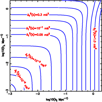
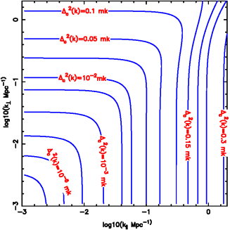
Figure 1: Figure showing the power spectrum in 3D redshift space at $z=2.5$. The left panel shows the HI 21-cm power spectrum $\Delta_{T}^{2}=k^{3}P_{TT}({\bf k})/2\pi^{2}$ and the right panel shows the 3D cross-correlation power spectrum $\Delta_{C}^{2}=k^{3}P_{T\mathcal{F}}({\bf k})/2\pi^{2}$. The redshift space distortion reveals as departure from spherical symmetry of the power spectrum. (Guha Sarkar et al. (2012))

We investigate the possibility of detecting the signal using the upcoming SKA-mid phase1 telescope and future Ly-$\alpha$ forest surveys with very high quasar number densities. Two separate telescopes named SKA-low and SKA-mid operating at two different frequency bands and will be constructed in Australia and South Africa respectively in two phases. For this work we consider the instruments SKA1-mid which will be built in phase 1. The instrument specifications such as the total number of antennae, antenna distribution, frequency coverage, total collecting area etc., have not been fixed yet and might change in future. We use the specifications considered in the ‘Baseline Design Document’ and ’SKA Level 1 Requirements (revision 6)’ which are available on the SKA website. We assume that the SKA1-mid will operate in the frequency range from $350\,{\rm MHz}$ to $14$ GHz. It shall have $250$ antennae of $7.5$ meters radius each. We use the baseline distribution given in (Villaescusa-Navarro et al., 2015b) (figure 6-blue line) for the calculation presented here. We note that, the baseline distribution used here is consistent with the projected antenna layout distribution with $40\%$, $54\%$, $70\%$, $81\%$ and $100\%$ of the total antennae are assumed to be enclosed within $0.4$ km, $1$ km, $2.5$ km, $4$ km and $100$ km radius respectively.

The fiducial redshift of $z=2.5$ is justified since the quasar distribution peaks in the range $2<z<3$. Only a smaller part of the quasar spectra corresponding to an approximate band $\Delta z\sim 0.4$ is used to avoid contamination from metal lines and quasar proximity effect. The cross-correlation can however only be computed in the region of overlap between the 21-cm signal and the Ly-$\alpha$ forest field.

The left panel of the figure (1) shows the dimensionless redshift space 21-cm power spectrum ($\Delta^{2}_{T}(k_{\perp},k_{||})=k^{3}P_{T}(k_{\perp},k_{||})/2\pi^{2}$) at $z=2.5$. We can see that the power spectrum is not circularly symmetric in the $(k_{||}$, $k_{\perp})$ plane. The asymmetry is related to the redshift space distortion parameter. The right panel of figure (1) shows the 21-cm and Ly-$\alpha$ cross-power spectrum.

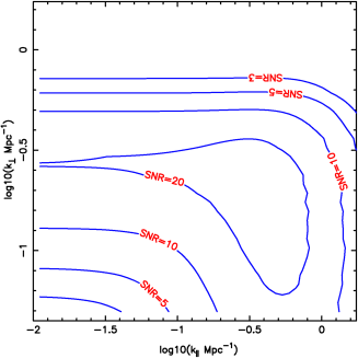
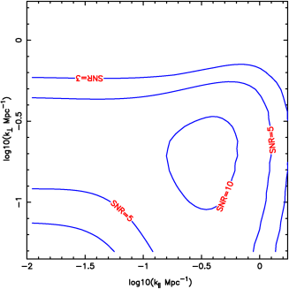
Figure 2: The left panel shows SNRcontours for the 21-cm auto-correlation power spectrum in redshift space at z = 2.5. We have considered a 400 hrs observation at 405 MHz and assumed that complete foreground cleaning is done. The right panel shows the SNR contours for the cross-correlation signal (Guha Sarkar et al. (2012))

.

We first consider that a perfect foreground subtraction is achieved. The left panel of the figure (2) shows the contours of SNR for the 21-cm auto correlation power spectrum for a $400\rm hrs$ observation and total $32$MHz bandwidth at a frequency $405.7\rm MHz$. We have taken a bin $(\Delta k,\Delta\theta)=(k/5,\pi/10)$. The SNR reaches at the peak ($>20$)at intermediate value of $(k_{\perp},k_{\parallel})=(0.4,0.4)\,{\rm Mpc^{-1}}$ . We find that $5\sigma$ detection is possible in the range $0.08\lesssim k_{\perp}\lesssim 0.6\,{\rm Mpc^{-1}}$ and $0.1\lesssim k_{\parallel}\lesssim 1.5\,{\rm Mpc^{-1}}$. The range for the $10\sigma$ detection is $0.12\lesssim k_{\perp}\lesssim 0.5\,{\rm Mpc^{-1}}$ and $0.2\lesssim k_{\parallel}\lesssim 1.2\,{\rm Mpc^{-1}}$. At lower values of $k$ the noise is expected to be dominated by cosmic variance whereas, the noise is predominantly of instrumental origin at large $k$.

The right panel of the figure (2) shows the SNR contours for the Ly-$\alpha$ 21-cm cross-correlation power spectrum. For the 21 cm signal, a $400\rm hrs$ observation is considered. We have taken $\bar{n}=30\rm deg^{-2}$, and the Ly-$\alpha$ spectra are assumed to be measured at a $2\sigma$ sensitivity level. We use $\beta_{F}$ to be $1.11$ and overall normalization factor $C_{\mathcal{F}}=-0.15$ consistent with recent measurements (Slosar et al., 2011b). Although the overall SNR for the cross power spectrum is lower compared to the 21-cm auto power spectrum, $5\sigma$ detection is ideally possible for the $0.1\lesssim k_{\perp}\lesssim 0.4\,{\rm Mpc^{-1}}$ and $0.1\lesssim k_{\parallel}\lesssim 1\,{\rm Mpc^{-1}}$. The SNR peaks ($>10$)at $(k_{\perp},k_{\parallel})\sim(0.2,0.3)\,{\rm Mpc^{-1}}$. The error in the cross-correlation can be reduced either by increasing the QSO number density or by increasing the observing time for HI 21-cm survey. The QSO number density is already in the higher side for the BOSS survey that we consider. The only way to reduce the variance is to consider more observation time for HI 21-cm survey and enhance the volume of the survey.

3.2 Parameter estimation using the cross-correlation

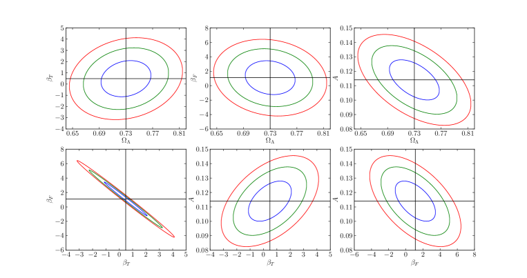
Figure 3: The $68.3\%,95.4\%$ and $99.8\%$ confidence ellipses for the parameters $(A,\beta_{T},\beta_{\mathcal{F}},\Omega_{\Lambda})$. (Guha Sarkar et al. (2012))

We now consider the precision at which we can constrain various model parameters using the Fisher matrix analysis. Figure (4) shows the $68.3\%,95.4\%$ and $99.8\%$ confidence contours obtained using the Fisher matrix analysis for the parameters $(A,\beta_{T},\beta_{\mathcal{F}},\Omega_{\Lambda})$. The table 1 summarises the $1-\sigma$ error these parameters. The parameters $(\Omega_{\Lambda},A)$ are constrained much better that $\beta_{\mathcal{F}}$ and $\beta_{T}$ at $(3.5\%,8\%)$. The error projections presented here are for a single field of view radio observation. The noise scales as $\sigma/\sqrt{N}$ where $N$ is the number of pointings.

Table 1: This shows $1-\sigma$ error on various cosmological parameters for a single field observation.

Parameters	Fiducial Value	$1\sigma$ Error	$1\sigma$ Error
		(marginalized)	(conditional)
$\beta_{T}$	0.48	1.06	0.04
$\beta_{\mathcal{F}}$	1.11	1.55	0.05
$\Omega_{\Lambda}$	0.73	0.025	0.013
$A$	0.114	0.01	0.002

We also consider conditional error on each of the parameters assuming that the other three are known. The projected $1-\sigma$ error in $\beta_{T}$ and $\beta_{\mathcal{F}}$ are $8.5\%$ and $4.5\%$ respectively for single pointing. For $10$ independent radio observations the conditional errors improve to $2.7\%$, $1.4\%$, $0.4\%$ and $0.6\%$ for $\beta_{T}$, $\beta_{\mathcal{F}}$, $\Omega_{\Lambda}$ and $A$ respectively. These constraints on the redshift space distortion parameters $\beta$ from our cross-correlation analysis are found to be quite competitive with other cosmological probes (Font-Ribera et al., 2012; Slosar et al., 2011a). Further, we note that higher density of QSOs and improved SNR for the individual QSO spectra shall also provide stronger constraints.

3.3 BAO imprint on the cross-correlation signal

The characteristic scale of the BAO is set by the acoustic horizon $s$ at the epoch of recombination The comoving length-scale $s$ defines a angular scale $\theta_{s}=s[(1+z)D_{A}(z)]^{-1}$ in the transverse direction and a radial redshift interval $\Delta z_{s}=sH(z)/c$, where $D_{A}(z)$ and $H(z)$ are the angular diameter distance and Hubble parameter respectively. The comoving acousic horizon scale $s=143\,\rm Mpc$ correspond to an angle $\theta_{s}=1.38^{\circ}$ and reshift interval $\Delta z_{s}=0.07$ at redshift $z=2.5$. Measurement of $\theta_{s}$ and $\Delta z_{s}$ separately, allows the determination of $D_{A}(z)$ and $H(z)$ separately and thereby constrain background cosmological evolution. Here we consider the possibility of measurement of these two parameters from the imprint of BAO features on the cross-correlation power spectrum.

The Fisher matrix is given by (Guha Sarkar & Bharadwaj, 2013)

$$F_{ij}=\frac{V}{(2\pi)^{3}}\int\,\,\frac{d^{3}{\bf k}}{[P^{2}_{\mathcal{F}T}({\bf k})+P_{\mathcal{F}\mathcal{F}o}({\bf k})P_{TTo}({\bf k})]}\frac{\partial P_{\mathcal{F}T}({\bf k})}{\partial q_{i}}\frac{\partial P_{\mathcal{F}T}({\bf k})}{\partial q_{j}}$$ (35)

where $q_{i}$ refer to the cosmological parameters to be constrained. This BAO signal is mainly present at small ${\bf k}$ (large scales) with the first peak at roughly $k\sim 0.045{\rm Mpc}^{-1}$. The subsequent oscillations are highly suppressed by $k\sim 0.3{\rm Mpc}^{-1}$ which is within the limits of the ${\bf k}_{\perp}$ and $k_{\parallel}$ integrals. We use $P_{b}=P-P_{c}$ to isolate the purely baryonic features, and we use this in $\partial P(k)/\partial q_{i}$. Here, $P_{c}$ is the CDM power spectrum without the baryonic features. This gives

$$P_{b}({\bf k})=\sqrt{8\pi^{2}}A\,\frac{\sin x}{x}\,\exp\left[-{\left(\frac{k}{k_{silk}}\right)}^{1.4}\right]\,\exp\left[{-\left(\frac{k^{2}}{2k_{nl}^{2}}\right)}\right]$$ (36)

where ${k_{silk}}$ and ${k_{nl}}$ denotes the scale of ‘Silk-damping’ and ‘non-linearity’ respectively. We have used $k_{nl}=(3.07\,h^{-1}\rm Mpc)^{-1}$ and $k_{silk}=(7.76\,h^{-1}\rm Mpc)^{-1}$ from (Seo & Eisenstein, 2007). The quantity $x=\sqrt{k_{\perp}^{2}s_{\perp}^{2}+k_{\parallel}^{2}s_{\parallel}^{2}}$ where $s_{\perp}$ and $s_{\parallel}$ corresponds to $\theta_{s}$ and $\Delta z_{s}$ in units of distance. $A$ is an overall normalization constant. The value of $s$ is well constrained from CMBR data. Changes in $D_{A}$ and $H(z)$ manifest as the corresponding changes in the values of $s_{\perp}$ and $s_{\parallel}$ respectively, and thus the fractional errors in $s_{\perp}$ and $s_{\parallel}$ correspond to fractional errors in $D_{A}$ and $H(z)$ respectively. We choose $q_{1}={\rm ln}(s_{\perp}^{-1})$ and $q_{2}={\rm ln}(s_{\parallel})$ as the cosmological parameters to be constrained, and determine the precision at which it will be possible to measure these using the BAO imprint on the in the cross-correlation power spectrum. We use the formalism outlined in (Seo & Eisenstein, 2007), whereby we construct the $2-D$ Fisher matrix

$$F_{ij}=VA^{2}\int dk\int_{-1}^{1}d\mu\frac{k^{2}\exp[-2(k/k_{silk})^{1.4}-(k/k_{nl})^{2}]}{[P_{\mathcal{F}T}^{2}(k)+P_{\mathcal{F}\mathcal{F}o}({\bf k})P_{TTo}({\bf k})/F^{2}_{\mathcal{F}T}(\mu)]}f_{i}(\mu)f_{j}(\mu)$$ (37)

$$F_{\mathcal{F}T}(\mu)=\frac{H(z)}{r^{2}c}C_{\mathcal{F}}C_{T}\,(1+\beta_{\mathcal{F}}\mu^{2})(1+\beta_{T}\mu^{2})$$ (38)

where $f_{1}=\mu^{2}-1$ and $f_{2}=\mu^{2}$. The Cramer-Rao bound $\delta q_{i}=\sqrt{F^{-1}_{ii}}$ is used to calculate the maximum theoretical error in the parameter $q_{i}$. A combined distance measure $D_{V}$, also referred to as the “dilation factor” (Eisenstein et al., 2005)

$$D_{V}(z)^{3}=(1+z)^{2}D_{A}(z)\frac{cz}{H(z)}$$ (39)

is often used as a single parameter to quantify BAO observations . We use $\delta D_{V}/D_{V}=\frac{1}{3}(4F^{-1}_{11}+4F^{-1}_{12}+F^{-1}_{22})^{0.5}$ to obtain the relative error in $D_{V}$. The dilation factor is known to be particularly useful when the individual measurements of $D_{A}$ and $H(z)$ have low signal to noise ratio.

The Fisher matrix formalism is used to determine the accuracy with which it will be possible to measure cosmological distances using this cross-correlation signal.

The limits $\bar{n}_{Q}\rightarrow\infty$ and $N_{T}\rightarrow 0$, which correspond to $P_{\mathcal{F}\mathcal{F}o}\rightarrow P_{\mathcal{F}\mathcal{F}}$ and $P_{TTo}\rightarrow P_{TT}$, set the cosmic variance limit. In this limit, where the SNR depends only on the survey volume corresponding to the total field of view we have $\delta D_{V}/D_{V}=0.15\%$, $\delta H/H=0.25\%$ and $D_{A}/D_{A}=0.15\%$ which are independent of any of the other observational details. The fractional errors decrease slowly beyond $\bar{n}_{Q}>50\rm deg^{-2}$ or $N_{T}<10^{-6}\rm mK^{2}$. We find that parameter values $\bar{n}_{Q}\sim 6\,\rm deg^{-2}$ and $N_{T}\sim 4.7\times 10^{-5}\ \rm mK^{2}$, attainable with BOSS and SKA1 mid are adequate for a $1\%$ accuracy, whereas $\bar{n}_{Q}\sim 2\,\rm deg^{-2}$ and $N_{T}\sim 3\times 10^{-3}\ \rm mK^{2}$ are adequate for a $\sim 10\%$ accuracy in measurement of $D_{V}$. With a BOSS like survey is possible to achieve the fiducial value $\delta D_{V}/D_{V}=2.0\%$ from the cross-correlation at $N_{T}=\,2.9\,\times\,10^{-4}{\rm mK}^{2}$. The error varies slower than $\sqrt{N_{T}}$ in the range $N_{T}=10^{-4}{\rm mK}^{2}$ to $N_{T}=10^{-5}{\rm mK}^{2}$. We have $(\delta D_{V}/D_{V},\delta D_{A}/D_{A},\delta H/H)=(1.3,1.5,1.3)\,\%$ and $(0.67,0.78,0.74)\,\%$ at $N_{T}=10^{-4}{\rm mK}^{2}$ and at $N_{T}=10^{-5}{\rm mK}^{2}$ respectively. The errors do not significantly go down much further for $N_{T}<10^{-5}{\rm mK}^{2}$, and we have $(0.55,0.63,0.63)\,\%$ at $N_{T}=10^{-6}{\rm mK}^{2}$.

3.4 Constraints on Neutrino mass

Free streaming of neutrinos causes a power suppression on large scales. This suppression of dark matter power spectrum shall imprint itself on the cross-correlation of Ly-$\alpha$ forest and 21 cm signal (Pal & Guha Sarkar, 2016). We have suggested this as a possible way to constrain neutrino mass. We have considered a BOSS like Ly-$\alpha$ survey with a quasar density of $30$ deg^-2 with an average $3\sigma$ sensitivity for the measured spectra. We have also assumed a 21 cm intensity mapping experiment at a fiducial redshift $z=2.5$ corresponding to a frequency $406$MHz using a SKA1-mid like instrument with 250 dishes each of diameter $15$m. We have assumed a $(\Omega_{\Lambda},\Omega_{m},\Omega_{r},h,\sum\nolimits_{i}m_{i})$=$(0.6825,0.3175,0.00005,0.6711,0.1{\rm ev})$ (Planck Collaboration et al., 2014) for this analysis. The Fisher matrix analysis using a two parameter $(\Omega_{m}.\Omega_{\nu})$ shows that For a 10.000 hrs radio observation distributed over 25 pointings of 400 hrs each the parameters $\Omega_{m}$ and $\Omega_{\nu}$ are measurable at $0.321\%$ and $3.671\%$. respectively [see figure (4)]. We find it significant that instead of a deep long duration observation in one small field of view, it is much better if one divides the total observation time over several pointings and thereby increasing survey volume. For 100 pointings each of $100hrs$ one can get a $2.36\%$ measurement of $\Omega_{\nu}$. This is close to the cosmic variance limit at the fiducial redshift and the given observations. In the ideal limit one may measure $\Omega_{\nu}$ at a $2.45\%$ level which corresponds to a measurement of $\sum m_{\nu}$ at the precision of $(0.1\pm 0.012)$ eV.

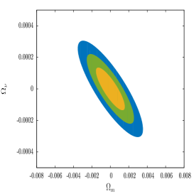
Figure 4: 68.3%,95.4% and 99.8% ellipse for 10000 hrs. observations for 25 pointings with each pointing of 400 hrs. observations. The marginalized one dimensional probability distribution function (PDF) (Pal & Guha Sarkar (2016)) for $\Omega_{m}$ and $\Omega_{\nu}$ are also shown.

4 Cross-correlation with Lyman break galaxies

The cross-correlation between the HI 21-cm signal and the Lyman break galaxies is another important tool to probe the large scale structure of the Universe at post reionization epoch. This has been studied recently (Villaescusa-Navarro et al., 2015b) using a high resolution N-body simulation. Prospects for detecting such a signal using the SKA1-mid and SKA1-low telescopes together with a Lyman break galaxy spectroscopic survey with the same volume have also been investigated. It is seen that the cross power spectrum can be detected with a SNR up to $\sim 10$ times higher than the HI 21-cm auto power spectrum. Like in all other cross power spectrum the Lyman break galaxy and HI 21-cm cross power spectrum is expected to be extracted more reliably from the much stronger by spectrally smoothed foreground contamination compared to the HI 21-cm auto power spectrum.

5 Cross-correlation of HI 21 cm signal with CMBR

5.1 Weak Lensing

Gravitational lensing has the effect of deflecting the CMBR photons. This forms a secondary anisotropy in the CMBR temperature anisotropy maps (Lewis & Challinor (2006)). The weak lensing of CMBR is a powerful probe the universe at distances ($z\sim 1100$) far greater than any galaxy surveys. Measurement of the secondary CMBR anisotropies, often uses the cross correlation of some relevant observable (related to the CMB fluctuations) with some tracer of the large scale structure (Hirata et al. (2004a); Smith et al. (2007); Hirata et al. (2004b)). For weak lensing statistics the ‘convergence’ and the ‘shear’ fields quantify the distortion of the maps due to gravitational lensing. Convergence ($\kappa$) measures the lensing effect through its direct dependence on the gravitational potential along the line of sight and is thereby a direct probe of cosmology. The difficulty in precise measurement of lensing is the need for very high resolutions in the CMBR maps, since typical deflections over cosmological scales is only a few arcminutes. The non-Gaussianity imprinted by lensing on smaller scales allows a statistical detection for surveys with low angular resolution. Cross-correlation with traces, limits the effect of systematics and thereby increases the signal to noise. The weak lensing observables like convergence are constructed using various estimators involving the the CMBR maps(T, E, B) (Seljak & Zaldarriaga (1999); Hu (2001); Hu & Okamoto (2002)). The reconstructed convergence field can then be used for cross correlation.

We have probed the possibility of using the post-reionization HI as a tracer of large scale structure to detect the weak lensing (Guha Sarkar, 2010) effects. We have studied the cross correlation between the fluctuations in the 21-cm brightness temperature maps and the weak lensing convergence field. We can probe the one dimensional integral effect of lensing at any intermediate redshift by tuning the observational frequency band for 21-cm observation. The cross-correlation power spectrum can hence independently quantify the cosmic evolution and structure formation at redshifts $z\leq 6$. The cross-correlation power spectrum may also be used to independently compare the various de-lensing estimators.

The distortions caused by the deflection is the quantity of study in weak lensing. At the lowest order, magnification of the signal is contained in the convergence. The convergence field is a line of sight integral of the matter over density $\delta$ given by (Van Waerbeke & Mellier (2003))

$$\kappa(\hat{\bf n})=\frac{3}{2}\Omega_{m0}{\left(\frac{H_{0}}{c}\right)}^{2}\int_{\eta_{0}}^{\eta_{LSS}}d\eta F(\eta)\delta(\mathcal{D}(\eta)\hat{\bf n},\eta)$$ (40)

and $F(\eta)$ is given by

$$F(\eta)=\frac{\mathcal{D}(\eta_{LSS}-\eta)\mathcal{D}(\eta)D_{+}(\eta)}{\mathcal{D}(\eta_{LSS})a(\eta)}$$ (41)

Here, $D_{+}$ denotes the growing mode of density contrast $\delta$, and $\eta_{LSS}$ denotes the conformal time to the epoch of recombination. The comoving angular diameter distance $\mathcal{D}(\chi)=\chi$ for flat universe, $\mathcal{D}(\chi)=\sin(K\chi)/K$ for $K=|1-\Omega_{m}-\Omega_{\Lambda}|^{1/2}H_{0}/c<0$ and $\mathcal{D}(\chi)=\sinh(K\chi)/K$ for $K>0$ Universe. The convergence power spectrum is defined as $\langle\ a_{\ell m}^{\kappa}a_{\ell^{\prime}m^{\prime}}^{\kappa*}\ \rangle=C_{\ell}^{\kappa}\delta_{\ell\ell^{\prime}}\delta_{mm^{\prime}}$. where $a_{\ell m}^{\kappa}$ are the expansion coefficients in spherical harmonic basis. The Convergence auto-correlation power spectrum for large $\ell$ can be approximated as

$$\mathcal{C}_{\ell}^{\kappa}\approx\frac{9}{4}\Omega_{m0}^{2}{\left(\frac{H_{0}}{c}\right)}^{4}\int d\eta\frac{F^{2}(\eta)}{\mathcal{D}^{2}(\eta)}P{\left(\frac{\ell}{\mathcal{D}(\eta)}\right)}$$ (42)

The cross correlation angular power spectrum between the post-reionization H i 21-cm brightness temperature signal and the convergence field, is given by

$${\mathcal{C}}_{\ell}^{HI-\kappa}=A(z_{\rm HI})\int dk\left[k^{2}P(k){\mathcal{I}}_{\ell}(kr_{\rm HI})\int d\eta F(\eta)j_{\ell}(kr)\right]$$ (43)

where $P(k)$ is dark matter power spectrum at $z=0$ , and

$${A}(z)=\frac{3}{\pi}\Omega_{m0}{\left(\frac{H_{0}}{c}\right)}^{2}\bar{T}(z)\bar{x}_{\rm HI}D_{+}(z)$$ (44)

We note that the convergence field $\kappa(\hat{\bf n})$, is not directly measurable in CMBR experiments. It is reconstructed from the CMBR maps through the use of various statistical estimators (Hanson et al. (2009); Kesden et al. (2003); Cooray & Kesden (2003)). The cross-correlation angular power spectrum, $\mathcal{C}_{\ell}^{HI-\kappa}$, does not de-lens the CMB maps directly. It uses the reconstructed cosmic shear fields , and is thereby very sensitive to the underlying tools of de-lensing, and the cosmological model. The cross-correlation angular power spectrum may provide a way to independently compare various de-lensing estimators.

The cross-correlation power spectrum follows the same shape as the matter power spectrum. The signal peaks at a particular $\ell$ which scales as $\ell\propto r_{\rm HI}$ when the redshift is changed. The angular distribution of power clearly follows the underlying clustering properties of matter. The amplitude depends on several factors which are related to cosmological model and the H i distribution at $z_{\rm HI}$. The angular diameter distances directly also depends directly on the cosmological parameters. The cross-correlation signal may hence be used independently for joint estimation of cosmological parameters.

We shall now discuss the prospect of detecting the cross-correlation signal assuming a perfect foreground removal. The error in the cross-correlation signal has the contribution due to instrumental noise and sample variance. Sample variance however puts a limiting bound on the detectability. The cosmic variance for $\mathcal{C}_{\ell}^{HI-\kappa}$ is given by

$$\sigma_{SV}^{2}=\frac{\mathcal{C}_{\ell}^{\kappa}\mathcal{C}_{\ell}^{HI}}{(2\ell+1){N_{c}}f_{s}\Delta\ell}$$ (45)

where $f_{s}$ is fraction of overlap portion of sky common to both observations. $N_{c}$ denotes the number of independent estimates of the signal.

In the ideal hypothetical possibility of a full sky 21 cm survey we have $f_{s}=1$, and used $\Delta\ell=1$. The predicted $S/N$ is found to be $\sim 2$ and is not significantly high for detection which requires $S/N\geq 3$. Choosing a $\Delta\ell=10$ for $\ell\leq 100$ and $\Delta\ell=100$ for $\ell>100$ shall produce a $S/N>3$. This establishes that, with full sky coverage and negligible instrumental noise, the binned cross-correlation power spectrum is not cosmic variance limited and it detectable. The $S/N$ estimate is based on H i observation at only one frequency. The $21$- cm observations allow us to probe a continuous range of redshifts. This allows us to further increase the $S/N$ by collapsing the signal from various redshifts. In principle, a broad band 21-cm experiment may further increase the $S/N$.

The $S/N$ maybe improved by collapsing the signal from different scales $\ell$ and thereby test the feasibility of a statistically significant detection. The cumulated SNR upto a multipole $\ell$ is given by

$${\left(\frac{S}{N}\right)}^{2}=\sum_{0}^{\ell}\frac{(2\ell^{\prime}+1){N_{c}}f_{s}{(\mathcal{C}_{\ell^{\prime}}^{HI-\kappa})}^{2}}{(\mathcal{C}_{\ell^{\prime}}^{HI}+N_{\ell^{\prime}}^{HI})(\mathcal{C}_{\ell^{\prime}}^{\kappa}+N_{\ell^{\prime}}^{\kappa})}$$ (46)

$N_{\ell}^{\kappa}$ and $N_{\ell}^{HI}$ denotes the noise power spectrum for $\kappa$ and H i observations respectively. Ignoring the instrument noises we note that there is a significant increase in the $S/N$ by cumulating over multipoles $\ell$. This implies that a statistically significant detection of $\mathcal{C}_{\ell}^{HI-\kappa}$ is possible and the signal is not limited cosmic variance. It is important to push instrumental noise to the limit set by cosmic variance for a detection of the signal. At the relevant redshifts of interest, it is possible to reach such low noise levels with SKA. It is however important to scan large parts of the sky and thereby increase the survey volume.

Instrumental noise plays an important role at large multipoles (small scale). For a typical CMB experiment, the noise power spectrum (Marian & Bernstein (2007); Smith et al. (2006)) is given by $N_{\ell}=\sigma^{2}_{\rm{pix}}\Omega_{\rm{pix}}{W_{\ell}}^{-2}$, where different pixels have uncorrelated noise with variance $\sigma^{2}_{\rm{pix}}=s^{2}/t_{\rm{pix}}$. Here $s^{2}$ and $t_{\rm{pix}}$ are the pixel sensitivity and ‘time spent on the pixel’ respectively. $\Omega_{\rm{pix}}$ is the solid angle subtended per pixel and we use a Gaussian beam $W_{\ell}=\rm{exp}[{-\ell^{2}\theta^{2}_{FWHM}/16ln2}]$.

For H i observations, the quantity of interest is the complex Visibility which is used to estimate the power spectrum (Ali et al. (2008)). For a radio telescope with N antennae, system temperature $T_{sys}$, operating at a frequency $\nu$, and band width $B$ the noise correlation is given by $N_{\ell}^{HI}\propto\frac{1}{N(N-1)}{\left[\frac{T_{sys}}{K}\right]}^{2}\frac{1}{T\sqrt{{\Delta\nu}B}}$.

Where $T$ denotes total observation time, and $K$ is related to the effective collecting area of the antenna dish. Binning in $\ell$ also reduces the noise. The bin $\Delta\ell=1/2{\pi}^{2}\theta_{0}$ is chosen assuming a Gaussian beam of width $\theta_{0}$. With a SKA like instrument (Ali et al. (2008)), one can attain a noise level much lesser than the signal by increasing the observation time (infact a 5000 hour observation with present SKA configuration is good enough) and also by increasing the radial distance probed bi increasing the band width of the telescope. Being inversely related to the total number of antennae in the radio array, future designs may actually allow further reduction of the the system noise and achieve $N_{\ell}^{HI}<<\mathcal{C}_{\ell}^{HI}$. This establishes the detectability of the cross-correlation signal. We would like to conclude by noting that correlation between weak lensing fields and 21 cm maps, quantified through $\mathcal{C}_{\ell}^{{HI}-\kappa}$ may allow an independent means to estimate cosmological parameters and also test various estimators for CMBR delensing.

5.2 ISW effect

In an Universe, dominated by the cosmological constant, $\Lambda$ , the expansion factor of the universe, $a$, grows at a faster rate than the linear growth of density perturbations. This consequently implies that, the gravitational potential $\Phi\propto-\delta/a$ will decay. The ISW effect is caused by the change in energy of CMB photons as they traverse these time dependent potentials.

If the horizon size at the epoch of dark energy dominance (decay of the potential) is represented by $\eta_{\Lambda}$, then the ISW effect is suppressed on scales $k\geq 2\pi/\eta_{\Lambda}$. This corresponds to an angular scale $\ell_{\Lambda}=2\pi d/\eta_{\Lambda}$, where $d$ is the angular diameter distance to the epoch of decay.

The ISW term in CMBR temperature anisotropy is given by

$$\Delta T(\hat{\bf n})^{\rm ISW}=2T\int_{\eta_{\rm{LSS}}}^{\eta_{0}}d\eta\eta\,\dot{\Phi}(r\hat{\bf n},\eta).$$ (47)

The cross correlation angular power spectrum between HI 21 cm signal and ISW is given by (Guha Sarkar et al., 2009)

$${\cal{C}}_{\ell}^{HI-ISW}={\cal{K}}(z_{\rm HI})\int dk(P(k)\cal{I}_{\ell}(kr_{\rm HI})\int_{\eta_{\rm LSS}}^{\eta_{0}}d\eta F(\eta)j_{\ell}(kr))$$ (48)

where $P(k)$ is the present day dark matter power spectrum,

$$\mathcal{K}(z)=-\bar{T}(z)\bar{x}_{\rm HI}D_{+}(z)\frac{6H_{0}^{3}\Omega_{m0}}{\pi c^{3}}$$ (49)

$${\mathcal{I}}_{\ell}(x)=bj_{\ell}(x)-f\frac{d^{2}j_{\ell}}{dx^{2}}$$ (50)

and

$$F(\eta)=\frac{D_{+}(f-1)H(z)}{H_{0}}$$ (51)

For large $\ell$ we can use the Limber approximation (Limber (1954); Afshordi et al. (2004)) which allows us to replace the spherical Bessel functions by a Dirac deltas as

$$j_{\ell}(kr)\approx\sqrt{\frac{\pi}{2\ell+1}}\delta_{D}(\ell+\frac{1}{2}-kr)$$

whereby the angular cross-correlation power spectrum takes the simple scaling of the form

$$\mathcal{C}_{\ell}^{HI-ISW}\sim\frac{\pi\mathcal{K}F}{2\ell^{2}}P(\frac{\ell}{r})$$ (52)

where $P(k)$ is the present day dark matter power spectrum and all the other terms on the rhs. are evaluated at $z_{\rm HI}$. The dimensionless quantity $f$ quantifies the growth of the dark matter perturbations, and the ISW effect is proportional to $f-1$. The term $f-1$ is a sensitive probe of dark energy. Here we estimate the viability of detecting the H i -ISW cross-correlation signal. Cosmic variance sets a limit in deciding whether the signal can at all be detected or not. Even in the cosmic variance limit at $z\sim 1.0$ with a 32 MHz observation we find that ${\rm S/N}<0.45$ for all $z_{\rm HI}$ and $\ell$ and a statistically significant detection is not possible in such cases. It is possible to increase ${\rm S/N}$ collapsing the signal at different multipoles $\ell$. To test if a statistically significant detection is thus feasible we have collapsed all multipoles less than $\ell$ to evaluate the cumulative ${\rm S/N}$ defined as (Cooray (2002); Adshead & Furlanetto (2008)) We find that the contribution in the cumulated $S/N$ comes from $\ell<50$ at all redshifts $0.4<z<2$. The cross-correlation signal is largest at ($z\sim 0.4$) and is negligible for ($z>3$). We further find that although there is an increase in ${\rm S/N}$ on collapsing the multipoles it is still less than unity. This implies that a statistically significant detection is still not possible. Thus, probing a thin shell of H i doesn’t allow us to detect a cross correlation, the signal being limited by the cosmic variance. A cumulated S/N of $\sim 1.6$ is attained for redshift upto $z=2$ and there is hardly any increase in S/N on cumulating beyond this redshift. This is reasonable because the contribution from the ISW effect becomes smaller beyond the redshift $z>2$. This S/N is the theoretically calculated value for an ideal situation and is unattainable for most practical purposes. Incomplete sky coverage, and foreground removal issues would actually reduce the S/N and attaining a statistically significant level is not feasible.

6 Acknowledgements

KKD would like to thank DST for support through the project SR/FTP/PS-119/2012. TGS would like to thank the project SR/FTP/PS-172/2012 for financial support.

References

- Adshead & Furlanetto (2008) Adshead P. J., Furlanetto S., 2008, Monthly Notices of Royal Astronomical Society, 384, 291.
- Afshordi et al. (2004) Afshordi N., Loh Y., Strauss M. A., 2004, Physical Review D, 69, 083524.
- Ali & Bharadwaj (2014) Ali S. S., Bharadwaj S., 2014, Journal of Astrophysics and Astronomy, 35, 157.
- Ali et al. (2008) Ali S. S., Bharadwaj S., Chengalur J. N., 2008, Monthly Notices of Royal Astronomical Society, 385, 2166.
- Alonso et al. (2015) Alonso D., Bull P., Ferreira P. G., Santos M. G., 2015, MNRAS, 447, 400.
- Bagla et al. (2010) Bagla J. S., Khandai N., Datta K. K., 2010, MNRAS, 407, 567.
- Bharadwaj & Sethi (2001) Bharadwaj S., Sethi S. K., 2001, Journal of Astrophysics and Astronomy, 22, 293.
- Bharadwaj et al. (2009) Bharadwaj S., Sethi S. K., Saini T. D., 2009, Physical Review D, 79, 083538.
- Bull et al. (2015) Bull P., Ferreira P. G., Patel P., Santos M. G., 2015, ApJ , 803, 21.
- Camera et al. (2013) Camera S., Santos M. G., Ferreira P. G., Ferramacho L., 2013, Phys. Rev. Lett. 111, 171302.
- Chang et al. (2008) Chang T., Pen U., Peterson J. B., McDonald P., 2008, Physical Review Letters, 100, 091303.
- Cooray (2002) Cooray A., 2002, Physical Review D, 65, 103510.
- Cooray & Kesden (2003) Cooray A., Kesden M., 2003, New Astronomy, 8, 231.
- Croft et al. (1999a) Croft R. A. C., Hu W., Davé R., 1999a, Physical Review Letters, 83, 1092.
- Croft et al. (1999b) Croft R. A. C., Weinberg D. H., Pettini M., Hernquist L., Katz N., 1999b, Astrophysical Journal, 520, 1.
- Delubac et al. (2014) Delubac T., et al., 2014, preprint, 1404.1801.)
- Di Matteo et al. (2002) Di Matteo T., Perna R., Abel T., Rees M. J., 2002, Astrophysical Journal,564, 576.
- Eisenstein et al. (2005) Eisenstein D. J., Zehavi I., Hogg D. W., Scoccimarro R., 2005, ApJ, 633, 560.
- Fan et al. (2006) Fan X., et al., 2006, Astron.J. 132, 117.
- Font-Ribera et al. (2012) Font-Ribera A., et al., 2012, J. Cosmol. Astropart. Phys. , 11, 59.
- Gallerani et al. (2006) Gallerani S., Choudhury T. R., Ferrara A., 2006, Monthly Notices of Royal Astronomical Society, 370, 1401.
- Ghosh et al. (2010) Ghosh A., Bharadwaj S., Ali S. S., Chengalur J., 2010, Submitted to MNRAS
- Ghosh et al. (2011) Ghosh A., Bharadwaj S., Ali S. S., Chengalur J. N., 2011, MNRAS, 418, 2584.
- Guha Sarkar (2010) Guha Sarkar T., 2010, Journal of Cosmology and Astro-Particle Physics, 2, 2.
- Guha Sarkar & Bharadwaj (2013) Guha Sarkar T., Bharadwaj S., 2013, J. Cosmol. Astropart. Phys., 8, 023.
- Guha Sarkar et al. (2009) Guha Sarkar T., Datta K. K., Bharadwaj S., 2009, Journal of Cosmology and Astro-Particle Physics, 8, 19.
- Guha Sarkar et al. (2011) Guha Sarkar T., Bharadwaj S., Choudhury T. R., Datta K. K., 2011, MNRAS, 410, 1130.
- Guha Sarkar et al. (2012) Guha Sarkar T., Mitra S., Majumdar S., Choudhury T. R., 2012, MNRAS, 421, 3570.
- Guha Sarkar et al. (2012) Guha Sarkar T., Datta K. 2015, JCAP, 8,1.
- Hanson et al. (2009) Hanson D., Challinor A., Lewis A., 2009, preprint, 0911.0612.)
- Hirata et al. (2004a) Hirata C. M., Padmanabhan N., Seljak U., Schlegel D., Brinkmann J., 2004a, Physical Review D, 70, 103501
- Hirata et al. (2004b) Hirata C. M., Padmanabhan N., Seljak U., Schlegel D., Brinkmann J., 2004b, Physical Review D, 70, 103501.
- Hu (2001) Hu W., 2001, Astrophysical Journal Letters, 557, L79.
- Hu & Okamoto (2002) Hu W., Okamoto T., 2002, Astrophysical Journal, 574, 566.
- Kesden et al. (2003) Kesden M., Cooray A., Kamionkowski M., 2003, Physical Review D, 67, 123507.
- Kim et al. (2007) Kim T., Bolton J. S., Viel M., Haehnelt M. G., Carswell R. F., 2007, Monthly Notices of Royal Astronomical Society, 382, 1657.
- Lanzetta et al. (1995) Lanzetta K. M., Wolfe A. M., Turnshek D. A., 1995, Astrophysical Journal, 440, 435.
- Lesgourgues et al. (2007) Lesgourgues J., Viel M., Haehnelt M. G., Massey R., 2007, Journal of Cosmology and Astro-Particle Physics, 11, 8.
- Lewis & Challinor (2006) Lewis A., Challinor A., 2006, Physics Reports, 429, 1.
- Limber (1954) Limber D. N., 1954, Astrophysical Journal, 119, 655.
- Loeb & Wyithe (2008) Loeb A., Wyithe J. S. B., 2008, Physical Review Letters, 100, 161301.
- Mandelbaum et al. (2003) Mandelbaum R., McDonald P., Seljak U., Cen R., 2003, Monthly Notices of Royal Astronomical Society, 344, 776.
- Marian & Bernstein (2007) Marian L., Bernstein G. M., 2007, MNRAS, 76, 123009.
- McDonald (2003) McDonald P., 2003, Astrophysical Journal, 585, 34.
- McDonald & Eisenstein (2007) McDonald P., Eisenstein D. J., 2007, Physical Review D, 76, 063009.
- McDonald et al. (2001) McDonald P., Miralda-Escudé J., Rauch M., Sargent W. L. W., Barlow T. A., Cen R., 2001, Astrophysical Journal, 562, 52.
- McQuinn & White (2011) McQuinn M., White M., 2011, MNRAS, 415, 2257.
- McQuinn et al. (2006) McQuinn M., Zahn O., Zaldarriaga M., Hernquist L., Furlanetto S. R., 2006, Astrophysical Journal, 653, 815.
- Myers et al. (2007) Myers A. D., Brunner R. J., Nichol R. C., Richards G. T., Schneider D. P., Bahcall N. A., 2007, Astrophysical Journal, 658, 85.
- Noterdaeme et al. (2009) Noterdaeme P., Petitjean P., Ledoux C., Srianand R., 2009, Astronomy and Astrophysics, 505, 1087.
- Pal & Guha Sarkar (2016) Pal A. K., Guha Sarkar T., 2016, MNRAS, 459.4, 3505-3511.
- Pâris et al. (2014) Pâris I., et al., 2014, Astronomy and Astrophysics, 563, A54.
- P’eroux et al. (2003) P’eroux C., McMahon R. G., Storrie-Lombardi L. J., Irwin M. J., 2003, MNRAS, 346, 1103.
- Planck Collaboration et al. (2014) Planck Collaboration et al., 2014, A A, 571, A16.
- Rauch (1998) Rauch M., 1998, ARAA, 36, 267.
- Santos et al. (2005) Santos M. G., Cooray A., Knox L., 2005, Astrophysical Journal, 625, 575.
- Seljak & Zaldarriaga (1999) Seljak U., Zaldarriaga M., 1999, Physical Review Letters, 82, 2636.
- Seo & Eisenstein (2007) Seo H.-J., Eisenstein D. J., 2007, ApJ, 665, 14.
- Slosar et al. (2011a) Slosar A., et al., 2011a, 9, 1.
- Slosar et al. (2011b) Slosar A., Font-Ribera A., Pieri M. M. e. a., 2011b, 9, 1.
- Smith et al. (2006) Smith K. M., Hu W., Kaplinghat M., 2006, 74, 123002.
- Smith et al. (2007) Smith K. M., Zahn O., Doré O., 2007, Physical Review D, 76, 043510
- Van Waerbeke & Mellier (2003) Van Waerbeke L., Mellier Y., 2003, ArXiv Astrophysics e-prints,
- Villaescusa-Navarro et al. (2014) Villaescusa-Navarro F., Viel M., Datta K. K., Choudhury T. R., 2014, JCAP, 9, 50.
- Villaescusa-Navarro et al. (2015a) Villaescusa-Navarro F., Viel M., Alonso D., Datta K. K., Bull P., Santos M. G., 2015a, 3, 034.
- Villaescusa-Navarro et al. (2015b) Villaescusa-Navarro F., Viel M., Alonso D., Datta K. K., Bull P., Santos M. G., 2015b, 3, 034.
- Wyithe (2008) Wyithe J. S. B., 2008, Monthly Notices of Royal Astronomical Society, 388, 1889.
- Wyithe & Loeb (2009) Wyithe J. S. B., Loeb A., 2009, Monthly Notices of Royal Astronomical Society, 397, 1926.
- Wyithe et al. (2008) Wyithe J. S. B., Loeb A., Geil P. M., 2008, 383, 1195.