Line of sight anisotropies in the Cosmic Dawn and EoR 21-cm power spectrum

Abstract

The line of sight direction in the redshifted 21-cm signal coming from the cosmic dawn and the epoch of reionization is quite unique in many ways compared to any other cosmological signal. Different unique effects, such as the evolution history of the signal, non-linear peculiar velocities of the matter etc will imprint their signature along the line of sight axis of the observed signal. One of the major goals of the future SKA-LOW radio interferometer is to observe the cosmic dawn and the epoch of reionization through this 21-cm signal. It is thus important to understand how these various effects affect the signal for it’s actual detection and proper interpretation. For more than one and half decades, various groups in India have been actively trying to understand and quantify the different line of sight effects that are present in this signal through analytical models and simulations. In many ways the importance of this sub-field under 21-cm cosmology have been identified, highlighted and pushed forward by the Indian community. In this article we briefly describe their contribution and implication of these effects in the context of the future surveys of the cosmic dawn and the epoch of reionization that will be conducted by the SKA-LOW.

1 Introduction

The ‘Cosmic Dawn’ (CD) is the period in the history of our universe when the first sources of light were formed and they gradually warmed up their surrounding intergalactic medium (IGM). This period was followed by the ‘Epoch of Reionization’ (EoR) when these first and subsequent population of sources produced enough ionizing photons to gradually change the state of most of the hydrogen in our universe from neutral (H i ​​) to ionized (H ii ​​). These two epochs possibly are the least known periods in the history of our universe. Our present understanding of these epochs is mainly constrained by the observations of the cosmic microwave background radiation (CMBR) (Komatsu et al., 2011; Planck Collaboration, 2015),the absorption spectra of the high redshift quasars (Becker et al., 2001; Fan et al., 2003; Becker et al., 2015) and the luminosity function and clustering properties of Ly$\alpha$ emitters (see e.g. Trenti et al. 2010; Ouchi et al. 2010; Bouwens 2016). These indirect observations are rather limited in their ability to answer many fundamental questions regarding these periods; e.g. the properties of these first sources of light and how they evolve as reionization progresses, precise duration and timing of the CD and the EoR, the relative contribution in the heating and ionization of the IGM from various types of sources, and the typical size and distribution of the heated and ionized regions. It is being anticipated that the currently ongoing and proposed future radio interferometric surveys of these epochs, through the brightness temperature fluctuations of the redshifted 21-cm signal originating due to the hyperfine transition in the neutral hydrogen, has the potential to answer most these fundamental questions.

The currently ongoing redshifted 21-cm radio interferometric surveys, being conducted using the GMRT (Paciga et al., 2013), LOFAR (Yatawatta et al., 2013; van Haarlem et al., 2013), MWA (Tingay et al., 2013; Bowman et al., 2013; Dillon et al., 2014) and PAPER (Parsons et al., 2014; Jacobs et al., 2015; Ali et al., 2015), are mainly aimed at detecting this signal from the EoR. Most of these instruments are not sensitive enough at high redshifts to detect this signal from the CD. The low frequency aperture array of the upcoming Square Kilometre Array (SKA-LOW) will be a significant step forward in this regard as it will have enough sensitivity over a large range of low frequencies to observe the redshifted 21-cm signal from both the CD and the EoR (Mellema et al., 2013; Koopmans et al., 2015). Also, it is worth mentioning that, while the first generation experiments aim to detect the signal through statistical estimators like variance and power spectrum (due to their limited sensitivity), the SKA-LOW is expected to be sensitive enough (owing to its large collecting area) to make images of fluctuations in H i from these epochs (Mellema et al., 2015).

However, as the redshifted 21-cm signal from the CD and the EoR has not been detected till date by any of these first generation telescopes and they so far only managed to provide somewhat weak upper limits on the signal power spectra (Paciga et al., 2013; Ali et al., 2015) at large length scales, so it has been planned that the first phase of the SKA-LOW will survey a large volume of the sky for a relatively shorter observation time to estimate the signal power spectrum at different redshifts, which will possibly constrain some of the main parameters of the signal (Koopmans et al., 2015). The spherically averaged power spectrum which is perceived as the main tool to achieve the first detection of the signal with the first generation instruments and the initial tool for the CD-EoR parameter estimation with the SKA-LOW, provides a high signal to noise ratio (SNR) by averaging the signal in spherical shells in Fourier space, while still preserving many important features of the signal. However, as the CD-EoR 21-cm signal is expected to be highly non-Gaussian in nature (Bharadwaj & Pandey, 2005; Mondal et al., 2015; Mondal et al., 2016b, a), thus the power spectrum alone cannot represent all the properties of such a field.

Even when one is dealing with the power spectra of the signal, one has to be aware of the fact that the line of sight (LoS) direction of the redshifted 21-cm signal is unique. As the 21-cm signal originates from a line transition, signal coming from different cosmological distances along the LoS essentially belongs to different epochs and gets redshifted to different wavelengths, characterized by their cosmological redshift $z$. This implies that the signal present in an actual observational data cube containing a range of frequencies or wavelengths will evolve in time along the frequency or LoS direction. This is popularly known as the light cone effect (Barkana & Loeb, 2006; Datta et al., 2012, 2014). Thus while analyzing the three dimensional data one has to take this into account for a proper interpretation of the signal.

Another effect which also affects the signal along the LoS direction is the non-random distortions of the signal caused by the peculiar velocities of the matter particles. The coherent inflows of matter into overdense regions and the outflows of matter from underdense regions will produce an additional red or blueshift in the 21-cm signal on top of the cosmological redshift, changing the contrast of the 21-cm signal, and making it anisotropic along the LoS. It has been first highlighted by Bharadwaj & Ali (2004, 2005) and Ali et al. (2005) that the peculiar velocities will significantly change the amplitude and the shape of the 21-cm power spectrum measured from the observations of the periods before, during and even after the reionization.

Ali et al. (2005) was also first to highlight another source of anisotropy along the LoS of the redshifted 21-cm signal from the CD and the EoR, which is caused due to the Alcock-Paczynski effect (Alcock & Paczynski, 1979). This is the anisotropy due to the non-Euclidean geometry of the space-time. It is important to take into account this effect when one wants to do parameter estimation using the CD-EoR 21-cm power spectrum.

The ‘bulk flows’, which could arise from possible supersonic relative velocities between dark matter and baryonic gas (Tseliakhovich & Hirata, 2010) can also contribute to the LoS anisotropy in the signal.

Understanding and quantifying the line of sight anisotropy (caused by several aforementioned reasons) in the CD-EoR 21-cm power spectrum has been one of the long standing important issues in 21-cm cosmology. This will be especially important in the context of the upcoming SKA-LOW observations, which will probably be the first instrument to have enough sensitivity to constrain the model parameters of both the CD and the EoR significantly using the 21-cm power spectrum. We have been very active for almost one and half decade in this sub-field under 21-cm cosmology. To be more precise, in the context of the 21-cm cosmology this sub-field was identified and highlighted by Bharadwaj et al. (2001); Bharadwaj & Ali (2004, 2005); Bharadwaj & Pandey (2005); Ali et al. (2005); Datta et al. (2007), through analytical models of the signal power spectrum. These analytical predictions were later tested, validated and further pushed forward by the same groups using various kinds of simulations (Choudhury et al., 2009; Datta et al., 2012; Majumdar et al., 2013; Jensen et al., 2013; Datta et al., 2014; Majumdar et al., 2014; Ghara et al., 2015a, b; Majumdar et al., 2016). In this article we aim to summarize the effects of line of sight anisotropy in the CD-EoR 21-cm power spectrum considering future SKA-LOW observations and our contribution in this subject.

The structure of this article is as follows. In Section 2, we briefly describe different sources that contribute to the LoS anisotropy of the signal. We next describe different methods to quantify the LoS anisotropy present in the power spectra in Section 3. In Sections 4 and 5 we describe how one would be able to quantify and interpret the two major sources of LoS anisotropy in the signal using the simulated expected signal at different era, for several ongoing experiments and as well as for the SKA-LOW. We further discuss several issues that may hinder the detection of the signal as well as the quantification of the anisotropy in it in Section 6. Finally, in Section 7, we summarize our review.

2 Line of sight anisotropies in the redshifted 21-cm signal from the CD and EoR

We briefly describe here the three major LoS anisotropies affecting the redshifted 21-cm signal originating from the cosmic dawn and the EoR.

2.1 Redshift space distortions

The fluctuations in the brightness temperature of the redshifted 21-cm radiation essentially trace the H i distribution during the CD and the EoR. In a completely neutral IGM the H i distribution is expected to follow the underlying matter distribution with a certain amount of bias, at large enough length scales. The coherent inflows of matter into overdense regions and the outflows of matter from underdense regions will produce an additional red or blue shift on top of the cosmological redshift. If we consider a distant observer located along the $x$ axis and use the $x$ component of the peculiar velocity to determine the position of H i particles in redshift space

$$s=x+\frac{v_{x}}{aH(a)}\,,$$ (1)

where $a$ and $H(a)$ are the scale factor and Hubble parameter respectively. Thus, in redshift space the apparent locations of the H i particles will change according to the above equation, which will effectively change the contrast of the 21-cm signal and will make it anisotropic along the LoS. However, as the first sources of lights were formed and they start converting their surrounding H i into H ii , the one-to-one correspondence between matter and H i no longer holds and the effect of the matter peculiar velocities on the 21-cm signal becomes much more complicated. In the context of the 21-cm signal from the CD and EoR, this effect was first pointed out and quantified in Bharadwaj & Ali (2004) and Bharadwaj & Ali (2005). Their analytical treatment showed that the redshift space distortions changes the shape and amplitude of the signal power spectrum significantly when measured from the recorded visibilities in a radio interferometric observation. It has also been proposed that one can possibly extract the matter power spectrum (Barkana & Loeb, 2005; Shapiro et al., 2013) at these epochs using the redshift space anisotropy present in the 21-cm power spectrum.

2.2 Light cone effect

The other LoS anisotropy that will be present in the observed 21-cm signal is known as the light cone anisotropy. As light takes a finite amount of time to reach from a distant point to an observer, thus the cosmological 21-cm signal coming from different cosmological redshifts essentially belongs to different distances and thus correspond to different cosmological epochs. In the context of redshifted 21-cm signal, this change in frequency due to cosmological redshift can be represented by

$$\lambda_{\rm obs}=\lambda_{\rm emitted}(1+z)\,.$$ (2)

Any radio interferometric observation produces a three dimensional data set containing a range of frequencies. The time evolution of the signal will be present in such a data set as one changes the frequency. Thus, while estimating power spectrum of the signal from such a data one needs take into account this effect for a proper interpretation of the signal. In the context of 21-cm signal this was first considered by Barkana & Loeb (2006) in their analytical estimation of the two point correlation function of the signal. This also makes the shape of the H ii regions around extremely bright sources (e.g. quasars) anisotropic along the LoS (Wyithe et al., 2005; Yu, 2005; Majumdar et al., 2011, 2012). If the reionization was dominated by such sources than the effect on power spectrum and correlation functions in such a case has been studied by Sethi & Haiman (2008). Such anisotropy in the shape of the H ii region can be detected by targeted tomographic imaging by deep observations around such sources using of the SKA-LOW (Majumdar et al., 2012). This has been discussed in further details in a different review article in this special issue.

2.3 Alcock-Paczynski effect

The Alcock-Paczynski effect (Alcock & Paczynski 1979, hereafter the AP effect), another anisotropy in the signal along the LoS, is caused due to the non-Euclidean geometry of the space-time. This makes any object, which is intrinsically spherical in shape, to appear elongated along the LoS. At low redshifts (for $z\leq 0.1$) it is not that significant but at high redshifts this causes a significant distortion in the signal, which makes the power spectrum of the 21-cm signal from the CD and the EoR anisotropic along the LoS. The AP effect in the context of 21-cm signal from the EoR was first considered by Ali et al. (2005) in their analysis of the signal through the power spectrum. The proposal of Barkana & Loeb (2005), that one can probably distinguish different sources that contribute to the 21-cm power spectrum by measuring the anisotropy in the power spectrum, has the implicit assumption that the background cosmological model is known to a great degree and hence does not take into account the anisotropies introduced by the geometry (AP effect). Ali et al. (2005) in contrast adopted a framework which allows the high redshift 21-cm signal to be interpreted without reference to a specific background cosmological model and also studied the variation in the anisotropy due to the AP effect depending on different background cosmological models. They further quantify the relative contribution in anisotropy due to the AP effect when compared with the anisotropy due to the redshift space distortions and how they differ in their nature. However, it has not been studied yet, how significant this effect will be when compared to the uncertainties due to the thermal noise and other systematics for a future SKA-LOW observation.

3 Methods to quantify the LoS anisotropy in 21-cm signal

We next discuss different possible ways of quantifying any line of sight anisotropy present in the signal through its power spectrum.

3.1 $\mu$-decomposition of the power spectrum

It is convenient to introduce a parameter $\mu$, defined as the cosine of the angle between a specific Fourier mode $\mathbf{k}$ and the LoS. In case of plane parallel redshift space distortions, the redshift space power spectrum then can be expressed as a fourth-order polynomial in $\mu$ (see e.g. Bharadwaj & Ali 2004, 2005; Ali et al. 2005; Barkana & Loeb 2005):

$$P^{\mathrm{s}}(k,\mu)=\overline{\delta T_{b}}^{2}(z)\left[P_{\mu^{0}}(k)+\mu^{2}P_{\mu^{2}}(k)+\mu^{4}P_{\mu^{4}}(k)\right]\,,$$ (3)

where $\overline{\delta T_{b}}$ is the average differential brightness temperature of the 21-cm signal at a specific redshift $z$. In the context of the CD and EoR 21-cm signal this representation of the power spectrum is popular, as one can directly identify each coefficients of the powers of $\mu$ with physical quantities contributing to the 21-cm power spectrum under the linear (Bharadwaj et al., 2001; Bharadwaj & Ali, 2004, 2005; Ali et al., 2005; Barkana & Loeb, 2005; Lidz et al., 2008; Majumdar et al., 2013) or quasi-linear (Mao et al., 2012; Jensen et al., 2013; Majumdar et al., 2014, 2016; Ghara et al., 2015a, b) model for the signal (which is valid mainly for the large scale fluctuations in the signal). Following this quasi-linear model one can express each of these coefficients of $\mu$ as:

$$P_{\mu^{0}}(k) =P_{\rho_{H{\sc I}},\rho_{H{\sc I}}}(k)+P_{\eta,\eta}(k)+P_{\rho_{H{\sc I}},\eta}(k)\,,$$

$$P_{\mu^{2}}(k) =2\left[P_{\rho_{H{\sc I}},\rho_{\mathrm{M}}}(k)+P_{\rho_{\mathrm{M}},\eta}(k)\right]\,,$$

$$P_{\mu^{4}}(k) =P_{\rho_{\mathrm{M}},\rho_{\mathrm{M}}}(k)\,.$$ (4)

where $\rho_{H{\sc I}}$ is the neutral hydrogen density, $\rho_{\mathrm{M}}$ is the total hydrogen density and $\eta(z,\mathbf{x})=1-T_{\mathrm{C}MB}(z)/T_{\mathrm{S}}(z,\mathbf{x})$ represents spin temperature fluctuations in the H i distribution. The spin temperature ($T_{\mathrm{S}}$), which represents the relative population of atoms in two different spin states, can get affected by the Lyman-$\alpha$ pumping and heating during the Cosmic Dawn and the early stages of reionization (Bharadwaj et al., 2001; Bharadwaj & Ali, 2004, 2005; Ali et al., 2005; Ghara et al., 2015a, b). For most part of the reionization, by when the IGM is expected to be significantly heated above the CMB temperature, it can be safely assumed that $T_{\mathrm{S}}\gg T_{\mathrm{C}MB}$ (unless it is a case of very late heating). In that case, all terms related to $\eta$ turns out to be zero and it becomes very tempting to conclude that at least at large scales this representation will hold and it would be possible to separate the astrophysics ($P_{\rho_{H{\sc I}},\rho_{H{\sc I}}}$ and $P_{\rho_{H{\sc I}},\rho_{\mathrm{M}}}$) from cosmology ($P_{\rho_{\mathrm{M}},\rho_{\mathrm{M}}}$). However, one has to be aware of the fact that this representation is not in orthonormal basis, thus each of these coefficients are not independent of the other, thus decomposing the power spectrum in this form and identifying the coefficients of the powers of $\mu$ with certain physical quantities may lead to erroneous conclusions. It is also important to note that this model do not consider any AP effect to be present in the signal, which will introduce an additional $\mu^{6}$ term in eq. (3) (Ali et al., 2005).

3.2 Legendre polynomial decomposition of the power spectrum

A different approach to quantify the LoS anisotropy is to instead expand the power spectrum in the orthonormal basis of Legendre polynomials, which is a well known approach in the field of galaxy redshift surveys (Hamilton, 1992, 1998; Cole et al., 1995). In this representation (assuming plane parallel redshift space distortions), the power spectrum can be expressed as a sum of the even multipoles of Legendre polynomials:

$$P^{\mathrm{s}}(k,\mu)=\sum_{l\;\mathrm{even}}{\mathcal{P}}_{l}(\mu)P_{l}^{\mathrm{s}}(k).$$ (5)

From an observed or simulated 21-cm power spectrum, one can calculate the angular multipoles $P_{l}^{\mathrm{s}}$ following:

$$P_{l}^{\mathrm{s}}(k)=\frac{2l+1}{4\pi}\int{\mathcal{P}}_{l}(\mu)P^{\mathrm{s}}(k)\mathrm{d}\Omega.$$ (6)

where ${\mathcal{P}}_{l}(\mu)$ represents different Legendre polynomials. The integral is performed over the entire solid angle to take into account all possible orientations of ${\bf k}$ with the LoS direction. Each multipole moment estimated through eq. (6) will be independent of the other, as this is a representation in orthonormal basis. In the context of 21-cm signal from the EoR, the effect of redshift space distortions was first quantified in Majumdar et al. (2013) by estimating the quadrupole ($P_{2}^{\mathrm{s}}$) and monopole ($P_{0}^{\mathrm{s}}$) moments of the power spectrum from EoR simulations. If one considers the quasi-linear model of the signal, the first three non-zero angular multipoles of the power spectrum can be expressed as (Majumdar et al., 2014, 2016):

$$P^{s}_{0} =\overline{\delta T_{b}}^{2}(z)\left[\frac{1}{5}P_{\rho_{\mathrm{M}},\rho_{\mathrm{M}}}+P_{\rho_{H{\sc I}},\rho_{H{\sc I}}}+P_{\eta,\eta}+2P_{\eta,\rho_{H{\sc I}}}\right.$$ (7)

$$\left.+\frac{2}{3}P_{\rho_{H{\sc I}},\rho_{\mathrm{M}}}+\frac{2}{3}P_{\eta,\rho_{\mathrm{M}}}\right]$$

$$P^{s}_{2} =4\,\overline{\delta T_{b}}^{2}(z)\left[\frac{1}{7}P_{\rho_{\mathrm{M}},\rho_{\mathrm{M}}}+\frac{1}{3}P_{\rho_{H{\sc I}},\rho_{\mathrm{M}}}+\frac{1}{3}P_{\eta,\rho_{\mathrm{M}}}\right]$$ (8)

$$P^{s}_{4} =\frac{8}{35}\,\overline{\delta T_{b}}^{2}(z)\,P_{\rho_{\mathrm{M}},\rho_{\mathrm{M}}}$$ (9)

This shows that it might be possible to extract the matter power spectrum by estimating the hexadecapole moment ($P_{4}^{\mathrm{s}}$) of 21-cm power spectrum for sufficiently large length scales. However, at those scales the signal might be severely dominated by the cosmic variance (see Section 6.2 for a detailed discussion). It further shows that, it is not possible to independently extract $P_{\rho_{H{\sc I}},\rho_{H{\sc I}}}$ or $P_{\rho_{H{\sc I}},\rho_{\mathrm{M}}}$, even when $T_{\mathrm{S}}\gg T_{\mathrm{C}MB}$ (i.e. when all $\eta$ related terms are zero).

3.3 Other alternative method

A simpler alternative method to quantify the LoS anisotropy in the signal power spectrum is to calculate the anisotropy ratio proposed by Fialkov et al. (2015), which is defined as:

$$r_{\mu}(k,z)=\frac{\langle P({\mathbf{k}},z)_{|\mu_{k}|>0.5}\rangle}{\langle P({\mathbf{k}},z)_{|\mu_{k}|<0.5}\rangle}-1\,,$$ (10)

where the angular bracket represent average over angles. Ideally, if the signal is isotropic then $r_{\mu}(k,z)$ should be zero, otherwise it will take positive or negative values. The redshift evolution of this quantity will some way quantify the integrated or angle averaged degree of anisotropy present in the signal at different stages of the CD and the EoR.

4 Quantifying the redshift space distortions in the 21-cm power spectrum

4.1 During the EoR

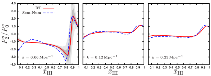
Figure 1: The evolution of the ratio $P^{s}_{2}/P^{s}_{0}$ with $\bar{x}_{{\rm H{\sc{I}}}}$ at three representative $k$ values estimated from a set of inside-out simulations of the EoR 21-cm signal (one semi-numerical and the other radiative transfer). The shaded regions in light and dark gray represent uncertainty due to the system noise for $2000$ and $5000$ hr of observation using a LOFAR like instrument at $150$ MHz. Figure taken from Majumdar et al. (2014).

The anisotropy in the redshifted 21-cm signal from the EoR has been traditionally quantified through the ratio of the spherically averaged power spectrum in redshift space to the same quantity estimated in real space. Predictions for this ratio has been made from analytical models as well as from radiative transfer and semi-numerical simulations of the signal (e.g. Lidz et al. 2007; Mesinger et al. 2011; Mao et al. 2012 etc.). However, one very important point to note here that, in reality one would not be able to estimate this ratio, as the signal will always have redshift space distortions present in it, thus it is not possible to estimate the power spectrum of the signal in real space. Instead of estimating this ratio, Majumdar et al. (2013) suggested that one could independently estimate different angular multipole moments of the power spectrum of the signal (following eq. [5] and [6]) directly from the observed visibilities, which is the basic observable in any radio interferometric survey. They further suggested that, the ratio between the first two non-zero even multipole moments of the power spectrum (i.e. monopole or $P^{s}_{0}$ and quadrupole or $P^{s}_{2}$) can be used as an estimator to quantify any LoS anisotropy present in the signal. It is precisely due to the fact that, if there is no LoS anisotropy in the signal, any higher order multipole moment, other than the monopole moment (which by definition is the spherically averaged power spectrum) will be zero. To quantify the effect of redshift space distortions in the signal Majumdar et al. (2013) used a set of semi-numerical simulations (with a proper implementation of the redshift space distortions in it using actual matter peculiar velocities) of the signal and studied the evolution of the ratio of $P^{s}_{2}/P^{s}_{0}$ with an evolving global neutral fraction ($\bar{x}_{{\rm H{\sc{I}}}}$) at different length scales observable to the present and future EoR surveys. They observed that at the early stages of the EoR ($1\gtrsim\bar{x}_{{\rm H{\sc{I}}}}\gtrsim 0.9$), for an inside-out reionization scenario, at large and intermediate length scales ($0.5\gtrsim k\gtrsim 0.05\,{\rm Mpc}^{-1}$), this ratio is positive and gradually goes up from the initial value of around $P^{s}_{2}/P^{s}_{0}=49/50$ (predicted by the linear model for a completely neutral IGM) to higher values ($\approx 3$ for $k\approx 0.05\,{\rm Mpc}^{-1}$ at $\bar{x}_{{\rm H{\sc{I}}}}\approx 0.9$) as reionization progresses further. Once the early stage of the EoR is over, one observes a sharp transition in this ratio at around $\bar{x}_{{\rm H{\sc{I}}}}\approx 0.9$, where it becomes negative and reaches values as low as $\approx-3$ at large length scales. It slowly goes up again with decreasing neutral fraction (for $0.5\lesssim\bar{x}_{{\rm H{\sc{I}}}}\lesssim 0.9$) and reaches a value of $-1$ by $\bar{x}_{{\rm H{\sc{I}}}}\approx 0.5$. This ratio remains negative and almost constant ($P^{s}_{2}/P^{s}_{0}\approx-1$) for the rest of the reionization ($\bar{x}_{{\rm H{\sc{I}}}}\leq 0.5$), until the signal strength goes down and it becomes undetectable. Majumdar et al. (2013) ascribes the sharp peak and dip features of the $P^{s}_{2}/P^{s}_{0}$ versus $\bar{x}_{{\rm H{\sc{I}}}}$ curve around $\bar{x}_{{\rm H{\sc{I}}}}\approx 0.9$ and negative value of $P^{s}_{2}/P^{s}_{0}$ for $\bar{x}_{{\rm H{\sc{I}}}}\leq 0.9$ to the inside-out nature of the reionization. The robustness of these results (and associated features in the behaviour of $P^{s}_{2}/P^{s}_{0}$) were further confirmed by Majumdar et al. (2014) by estimating the same ratio from a radiative transfer and a set of semi-numerical simulations (Figure 1). They also showed that this ratio would be detectable using LOFAR after $2000$ hr of observations. As these features of this ratio appears to be model invariant, so it can be used as a confirmative test for the detection of the signal. Both of the above mentioned studies also find that the hexadecapole moment ($P^{s}_{4}$) will be severely dominated by cosmic variance and thus it would be difficult to conclude anything about the matter power spectrum through it.

In a similar study with a radiative transfer simulation, but using the $\mu$-decomposition technique described in Section 3 through eq. (3), Jensen et al. (2013) also found that it is not possible to extract the coefficients of $\mu^{2}$ and $\mu^{4}$ terms in the signal power spectrum, i.e. not possible to extract $P_{\rho_{H{\sc I}},\rho_{\mathrm{M}}}$ and $P_{\rho_{\mathrm{M}},\rho_{\mathrm{M}}}$ independently, rather it is possible to extract the sum of the coefficients of $\mu^{2}$ and $\mu^{4}$, though it to would be more prone to errors compared to estimating the quadrupole moment ($P^{s}_{2}$) of the power spectrum, as it is a representation in non-orthonormal basis.

4.1.1 Constraining the EoR history using the redshift space anisotropy in the 21-cm signal

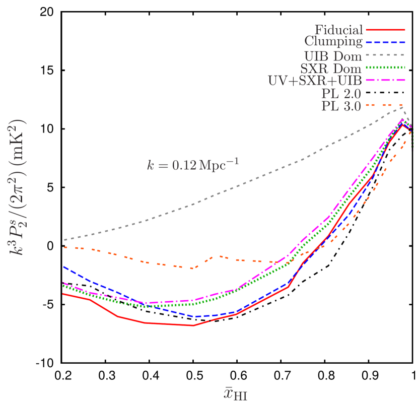
Figure 2: The quadrupole moment of the power spectrum for different reionization scenarios as a function of the global neutral fraction at $k=0.12$ Mpc^-1. Figure taken from Majumdar et al. (2016).

The quasi-linear model in eq. (8) suggest that the quadrupole moment ($P^{s}_{2}$) contains matter power spectrum and the cross-power spectrum between the matter and H i (when $T_{\mathrm{S}}\gg T_{\mathrm{C}MB}$, i.e. all $\eta$ related terms are zero). While the matter power spectrum contains the amplitude of the matter density fluctuations (which evolves rather slowly with redshift), the cross-power spectrum $P_{\rho_{H{\sc I}},\rho_{\mathrm{M}}}$ contains the information of the phase difference between the matter and the H i field. If the distribution and the properties of the reionization sources change, the topology of the ionization field will also change and one would expect then the phase difference between the matter and the H i field to also change, which it turn should have a signature in the quadrupole moment. To test whether this idea can be used to distinguish between different reionization sources using the nature and amplitude of $P^{s}_{2}$, Majumdar et al. (2016) simulated a collection of reionization scenarios considering various degrees of contribution from different kinds of reionization sources. The reionization scenarios they considered include ionizing photon contribution from the usual UV photon sources hosted by the halos with mass $\gtrsim 10^{9}\,{\rm M_{\odot}}$, a uniform ionizing background generated by hard X-ray sources, a local uniform ionizing background generated by soft X-ray sources (limited by the mean free path of soft X-ray photons), various combinations of all of these three contributions, reionization driven by quasar like very strong sources located around the most massive halos etc. They find that, for all of their reionization scenarios (except the one dominated by a uniform ionizing background), the quadrupole moment at large length scales ($k=0.12$ Mpc^-1) evolves with $\bar{x}_{{\rm H{\sc{I}}}}$ in a rather robust manner (Figure 2), even though the topology of the 21-cm signal look significantly different in all of those scenarios. They further show that as long as the major ionizing photon sources follow the underlying matter distribution, the phase difference between the matter and the H i evolves with $\bar{x}_{{\rm H{\sc{I}}}}$ in almost similar fashion, though the topology of the 21-cm signal can be drastically different. This is why the quadrupole moment ($P^{s}_{2}$) evolves in a robust fashion with $\bar{x}_{{\rm H{\sc{I}}}}$ in all of those scenarios. Building on this idea, they further demonstrate that this robustness of $P^{s}_{2}$ can be used to extract the reionization history to a great degree. They show that for an instrument with the sensitivity of the first phase of the SKA-LOW, it will require $100$ hr (per pointing) of observation over an area of minimum $5\times 5\,{\rm deg}^{2}$ in the sky to constrain the reionization history ($\bar{x}_{{\rm H{\sc{I}}}}$ versus $z$) very precisely, if foregrounds have already been removed to a great degree.

4.2 During the Cosmic Dawn

The 21-cm signal from the Cosmic Dawn and the very early stages of the EoR ($\bar{x}_{{\rm H{\sc{I}}}}\gtrsim 0.95$) are expected to be affected by the spin temperature fluctuations caused by the inhomogeneous X-ray heating and Lyman-$\alpha$ coupling around the early sources of light. In this regime one would not be able to assume $T_{\mathrm{S}}\gg T_{\mathrm{C}MB}$ and the fluctuations in the quantity $\eta(z,\mathbf{x})=1-T_{\mathrm{C}MB}(z)/T_{\mathrm{S}}(z,\mathbf{x})$ will contribute to the 21-cm brightness temperature significantly as predicted by Bharadwaj et al. (2001); Bharadwaj & Ali (2004, 2005); Ali et al. (2005) etc. Ghara et al. (2015a) developed and used an one dimensionals radiative transfer simulation to study the effects of spin temperature fluctuations on the 21-cm power spectrum during these stages while implementing the effect of redshift space distortions in the signal using the actual matter peculiar velocities. It was assumed that each of the early sources of light produced in their simulation has two components: i) usual stellar component (modelled using general population synthesis prescriptions) and ii) a mini-quasar component (assumed to have a power-law spectrum). They found some distinct features in the large scale power spectrum in this case when compared to the scenario where inhomogeneities in the gas temperature and the Lyman-$\alpha$ coupling are ignored. They observed three distinct peaks in the large scale spherically averaged power spectrum of the signal (which has been reported earlier in the literature e.g. see Pritchard & Loeb 2008) when plotted as a function of redshift (left panel of Figure 3). The peak which appears latest in the history is associated with $\sim 50\%$ neutral fraction of the IGM and the H i fluctuations have the maximum contribution to the power spectrum at this stage. The second peak is related to the fluctuations in the heating pattern and appears when $\sim 10\%$ of the volume is heated above $T_{\rm CMB}$. The third peak, which corresponds to the earliest stages of the 21-cm history, corresponds to the inhomogeneities in the Lyman-$\alpha$ coupling. Identification of these peaks (two of which were not reported earlier in the literature) would be very important when one would try to parametrize the CD and the EoR using the observed power spectrum and variance of the 21-cm signal from the proposed shallow survey ($10$ hr observation covering $10,000\,{\rm deg^{2}}$) using the first phase of SKA-LOW (Koopmans et al., 2015).

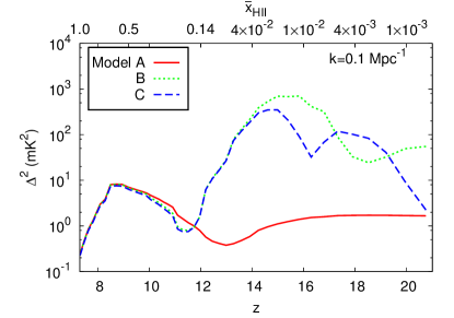
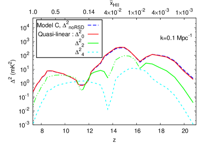
Figure 3: The left panel shows the spherically averaged 21-cm power spectrum at large length scales for three different models of X-ray heating and Lyman-$\alpha$ coupling. Model A: IGM is Lyman-$\alpha$ coupled and highly heated, Model B: IGM is strongly Lyman-$\alpha$ coupled but self consistently heated with X-ray sources, Model C: IGM is self consistently coupled with Lyman-$\alpha$ and heated by X-ray sources. The right panel shows the redshift space $\mu$-decomposed power spectra estimated following eq. (3) for Model C. Figure taken from Ghara et al. (2015a).

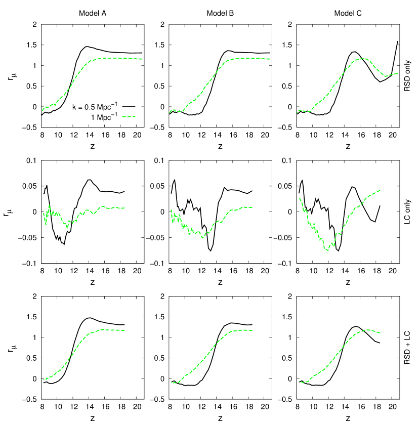
Figure 4: This shows the anisotropy ratio $r_{\mu}$ computed following eq. (10) as a function of redshift for large and intermediate length scales. The models A, B and C are the same as described in Figure 3, the only difference here is that all of them also include sources of mass lower than $10^{9}\,{\rm M_{\odot}}$. The three rows from top to bottom shows the ratio computed when the signal includes only the redshift space distortions, only light cone effect and both redshift space distortions and light cone effect, respectively. Figure taken from Ghara et al. (2015b).

To quantify the effect of redshift space distortions Ghara et al. (2015a) estimated the ratio of the spherically averaged power spectrum in redshift space and in real space. They find that this ratio at large length scales to be not that high as reported by some earlier studies (Majumdar et al., 2013; Jensen et al., 2013), when one includes the effect of spin temperature fluctuations. They associate this disagreement to the fact that they do not include the sources with mass lower than $10^{9}\,{\rm M_{\odot}}$ and also to the fact that during the CD and the early stages of the EoR the fluctuations in 21-cm are mainly driven by the fluctuations in $T_{\rm S}$, which is mildly correlated to the density field, thus the redshift space distortions do not change the amplitude and shape of the power spectrum drastically here. They have also estimated the $\mu$-decomposed power spectrum (right panel of Figure 3) following eq. (3) to further understand the effect of redshift space distortions on the signal power spectrum. They find that both the coefficients of $\mu^{2}$ and $\mu^{4}$ have non-zero values during this stage, however their amplitude are smaller or comparable but not higher than the coefficient of $\mu^{0}$ term (which is equivalent to the real space power spectrum) in the power spectrum. In a later work, Ghara et al. (2015b) have computed the anisotropy ratio (top panels of Figure 4) defined by eq. (10) as a function of $z$ at large and intermediate length scales ($k=0.1$ and $0.5\,{\rm Mpc}^{-1}$) for the similar reionization scenarios as in Ghara et al. (2015a) but here they have also included the sources of mass lower than $10^{9}\,{\rm M_{\odot}}$. It is evident from these figures that the anisotropy due to the redshift space distortions can be significant ($r_{\mu}\geq 1$) at large and intermediate length scales even during the Cosmic Dawn and the early stages of the EoR when one takes into account the inhomogeneities in the X-ray heating and Lyman-$\alpha$ coupling.

5 Quantifying the light cone effect in the 21-cm power spectrum

5.1 During the EoR

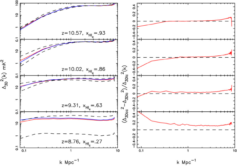
Figure 5: The left panels show the spherically averaged 21-cm power spectrum estimated from the light cone cube (LC:red solid line) and coeval cube at the central redshift (CC:blue solid line) at different stages of the EoR. The dashed lines show the power spectrum from the coeval cubes at redshifts corresponding to the back and the front sides of the light cone box. The right panels show the relative difference in the power spectra between the LC and the CC boxes, estimated at the same stages of the EoR as shown on the left. Figure taken from Datta et al. (2012).

The first numerical investigation of the light cone effect on the 21-cm power spectrum from the EoR was done by Datta et al. (2012). They used a set of radiative transfer simulations of volume $(163\,{\rm Mpc})^{3}$ having three different reionization histories (from rapid to slow) to study the light cone effect. They have quantified the impact of the light cone effect by estimating the relative difference between the spherically averaged power spectrum of the light cone box [$\Delta^{2}_{{\rm LC}}(k)$] and the same estimated from a coeval cube [$\Delta^{2}_{{\rm CC}}(k)$], corresponding to the central redshift of the light cone box, i.e. through the quantity $[\Delta^{2}_{{\rm CC}}(k)-\Delta^{2}_{{\rm LC}}(k)]/\Delta^{2}_{{\rm LC}}(k)$ (Figure 5). They observed that the relative change in the power spectrum can be up to $\approx 50\%$ within the $k$ range $\sim 0.1-9.0\,{\rm Mpc}^{-1}$ and the large scales are affected more compared to the small scales. They find that the light cone power spectrum get enhanced at large scales and suppressed at small scale compared to the coeval box power spectrum at the redshift of the centre of the box. This enhancement and suppression of power happens around a Fourier mode $k_{\rm cross-over}$, which gradually shifts towards the large scales as reionization progresses. Using simple toy models of power spectra, they argue that this behaviour is a signature of the difference in the bubble size distribution in the coeval box and the light cone box. They also observed that the difference in between $\Delta^{2}_{{\rm LC}}$ and $\Delta^{2}_{{\rm CC}}$ is minimum when reionization is half way through. The line of sight extent of the light cone box influences the difference between $\Delta^{2}_{{\rm LC}}$ and $\Delta^{2}_{{\rm CC}}$. This difference goes down with the reduction of the LoS extent of the light cone box. It was also noticed that as any radio interferometric observation do not measure the $k_{\perp}=0$ mode, thus the DC value of the signal power spectrum cannot be measured, which in turn removes the effect of the evolution of mass averaged neutral fraction ($\bar{x}_{{\rm H{\sc{I}}}}$) (across the LoS) from the observed light cone power spectrum. Datta et al. (2012) have further observed that the change in reionization history (whether rapid or slow), does not change the light cone affect on the power spectrum significantly. The light cone effect is more dependent on the mass averaged neutral fraction at the central redshift of the light cone box rather than the total EoR history. These findings of Datta et al. (2012) regarding the light cone effect were later confirmed independently by La Plante et al. (2014) as well.

It is intriguing to ask the question, whether the light cone effect introduces any significant LoS anisotropy to the observed EoR 21-cm power spectrum. If the anisotropy introduced by the light cone effect is significant and also contributes in a similar fashion in the power spectrum as the redshift space anisotropy, then it would be really difficult to distinguish between these two effects from a real observation. Also, several other proposed outcomes using the SKA-LOW observations, which uses the redshift space anisotropy as a tool, such as separating the cosmology from astrophysics (Barkana & Loeb, 2005) or extracting the reionization history (Majumdar et al., 2016), would be difficult to achieve. Datta et al. (2014) have tried to address mainly this issue, i.e. whether the light cone effect introduces any significant anisotropy to the signal power spectrum and what could be the best observational strategy to minimize the impact of the light cone effect on the EoR 21-cm power spectrum.

Datta et al. (2014) used a significantly large simulation volume ($[607\,{\rm Mpc}]^{3}$), which is comparable to the field of view of LOFAR, to study the impact of the light cone effect on the signal. The large simulation volume allowed them to study this effect in case of both very rapid as well rather slow reionization histories. They find the impact of the light cone effect on the spherically averaged power spectrum is maximum when the reionization is $\sim 20\%$ and $\sim 80\%$ finished and it is rather small at $\sim 50\%$ reionization. Which, reconfirms the findings of Datta et al. (2012). However, they do not observe any significant LoS anisotropy introduced to the power spectrum due to the light cone effect. They used a toy model to explain this rather surprising finding. They find that, even though the light cone effect makes the H ii bubbles larger in an observational data cube towards the side closer to the observer compared to the opposite side of the observational volume along the LoS, it does not necessarily makes the H ii bubbles elongated or compressed along the LoS. This systematic change in H ii bubble size along the LoS does not make the power spectrum anisotropic as long as the bubbles remain approximately spherical in shape. The power spectrum can only become anisotropic when the shape of the individual H ii bubbles distort along the LoS, which can only happen if the major sources of reionization are extremely strong in terms of their photon emission rate (e.g. quasars), which will lead to a relativistic growth of the H ii regions. They also studied the power spectrum by including both redshift space distortions and light cone effect to the signal and found that the light cone effect does not change the signatures of the redshift space distortions at any stage of the EoR.

Datta et al. (2014) also identified that there exists an optimal frequency bandwidth along the LoS for the power spectrum estimation, within which the light cone effect can be ignored without loosing the signal to the uncertainties due to the sample variance. They found that for large scales such as $k=0.16\,{\rm Mpc}^{-1}$ this is $\sim 11$ MHz and for intermediate scales $k=0.41\,{\rm Mpc}^{-1}$ this is $\sim 16$ MHz, if one allows a change of $10\%$ in the power spectra. These optimal bandwidths may change depending on the reionization history.

5.2 During the Cosmic Dawn

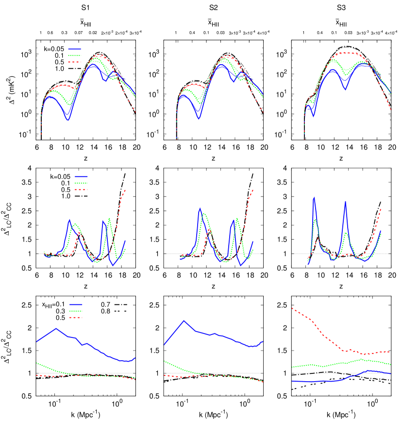
Figure 6: The top panels show evolution of the spherically averaged 21-cm power spectrum with redshift from simulation boxes with (thin line) and without (thick line) light cone effect in them. The middle and the bottom panels show relative change in the power spectrum due to the light cone effect when compared with the coeval power spectra. Three different columns correspond to three different models for reionization sources. Figure taken from Ghara et al. (2015b).

Ghara et al. (2015b) performed the first numerical study on the impact of the light cone effect on the redshifted 21-cm power spectrum from the Cosmic Dawn. They used a set of one dimensional radiative transfer simulations (similar to Ghara et al. 2015a) for the signal, while considering spin temperature fluctuations in the signal due to the inhomogeneous X-ray heating by the first sources and non-uniform Lyman-$\alpha$ coupling. They found that the impact of the light cone effect is more dramatic when one considers both the inhomogeneous X-ray heating and the Lyman-$\alpha$ coupling induced spin temperature fluctuations in the signal, compared to the case when these effects are ignored. It was observed that at large length scales $k\sim 0.05\,{\rm Mpc}^{-1}$, light cone effect is more prominent around the peaks and dips of the power spectrum when plotted as a function of redshift (Figure 6). They observed that the large scale signal power spectrum is suppressed around the three distinct peaks (by factors of $\approx 0.7$) and enhanced (by factors of $\approx 2$) around the dips due to this effect. This enhancement/suppression was found to be higher in a case where one includes sources of mass lower than $10^{9}\,{\rm M_{\odot}}$ in their reionization prescription. A significant light cone effect was also observed at small length scales ($k\sim 1\,{\rm Mpc}^{-1}$), during the Cosmic Dawn.

The reason behind this behaviour is that where ever the power spectrum experiences any non-linear evolution, the light cone effect becomes substantial at those points, as any linear evolution will be mostly cancelled out (Datta et al., 2012). This is possibly why this effect appears to be more prominent around the heating peak and the peak and dip caused due to the inhomogeneous Lyman-$\alpha$ coupling. It was also observed that inclusion or exclusion of light cone effect changes the power spectrum at large scales ($k\sim 0.05\,{\rm Mpc}^{-1}$) by $-100$ to $100\,{\rm mK}^{2}$ and at small scales ($k\geq 0.5\,{\rm Mpc}^{-1}$) by $-250$ to $100\,{\rm mK}^{2}$. These large differences should be in principle detectable by SKA-LOW, due to its higher sensitivity. It was proposed that the power spectrum peaks at large scales during the CD can be used to extract the source properties, X-ray and Lyman-$\alpha$ backgrounds etc (Mesinger et al., 2014). However, while performing such an exercise on an actual observational data set, one needs to take into account the light cone effect as it suppresses those peaks.

Similar to Datta et al. (2014) in the EoR, Ghara et al. (2015b) also did not find any significant LoS anisotropy introduced by the light cone effect in the signal from the CD. They had estimated the anisotropy ratio $r_{\mu}$ for large and intermediate scales (Figure 4) to quantify the LoS anisotropy due to the light cone effect. They found that the LoS anisotropy quantified by this ratio is less than $5\%$ during most of the duration of the CD and the EoR. They had also observed that, the light cone anisotropy do not destroy the anisotropy due to the redshift space distortions present in the signal.

6 Detectability of the line of sight anisotropy signatures

6.1 Foreground avoidance versus foreground removal

One of the major obstacle for the detection of the CD-EoR 21-cm signal is the foreground emission from galactic and extra-galactic point sources, which is expected to be few orders of magnitude larger than the signal itself. These foregrounds are assumed to be spectrally smooth, which implies that they will only affect the lowest $k$ modes parallel to the LoS ($k_{\parallel}$). However, due to the frequency dependence of an interferometers’s response, the foregrounds will propagate into higher $k$ modes. This causes the foregrounds to become confined to a wedge-shaped region in $k_{\parallel}-k_{\perp}$ plane, which was first identified by Datta et al. (2010). One of the ways to deal with the foregrounds is thus to avoid this region where foregrounds will be dominant and restrict the signal power spectrum estimation within the region of the $k_{\parallel}-k_{\perp}$ space which is expected to be clean from foregrounds (see e.g. Trott et al. 2012; Dillon et al. 2014; Pober et al. 2014 etc). One drawback of this method is that one have to live with the low SNR of the signal power spectrum, after throwing away a large fraction of the data in this way. The other drawback will be that the directional dependence of the power spectrum will be hard to quantify in this method. Detectability of any LoS anisotropy (more precisely the anisotropy due to the redshift space distortions in this context) present in the 21-cm signal power spectrum will depend on the fact that the power spectrum is sampled uniformly over all angles (or $\mu$ values) with respect to the LoS. Any sort of biased sampling of the power spectrum in this regard may lead to misinterpretation of signal characteristics and the related characteristics of the CD-EoR parameters. This would be inevitable in this foreground avoidence technique (Pober, 2015). Even when one is interested only in the spherically averaged power spectrum, it has been observed that the biased sampling of the $k_{\parallel}-k_{\perp}$ plane will introduce an atrificial but significantly large bias to the estimated power spectrum (Jensen et al., 2016). Thus to quantify the LoS anisotropies in the CD-EoR 21-cm signal using the future SKA-LOW shallow or medium survey (Koopmans et al., 2015), it is very important that we employ a proper foreground subtraction technique rather than using foreground avoidance.

6.2 Uncertainties due to the cosmic variance

Any statistical estimation of the CD-EoR 21-cm power spectrum comes with an intrinsic uncertainty of its own, which arises due to the uncertainties in the signal across its different statistically independent realizations, i.e. due to the cosmic variance of the signal. In most of the analysis present in the current literature related to the characterization of the CD-EoR 21-cm signal power spectrum, it has been assumed that the signal has properties similar to a Gaussian random field, which makes its cosmic variance to scale as the square root of the number of independent measurements. This could be a reasonably good assumption during the early phases of reionization, but during the later stages of the EoR, the signal becomes highly non-Gaussian as it gets characterized by the H ii regions around the reionization sources (Bharadwaj & Ali, 2005; Bharadwaj & Pandey, 2005). The size and population of these H ii regions gradually grow as reionization progresses, making the signal more and more non-Gaussian. A similar picture can be drawn during the early stages of the cosmic dawn as well, when the signal is characterized by the heated regions around the first sources of light. Using a large ensemble of simulated EoR 21-cm signal, Mondal et al. (2015) was the first to study the impact of the non-Gaussianity of this signal on the cosmic variance of its power spectrum estimation. They had shown that for a fixed observational volume it is not possible to obtain an SNR above a certain limit [SNR]_l, even when one increases the number of Fourier modes for the estimation of the power spectrum. This limiting SNR stays approximately in the range [SNR]${}_{l}\sim 500$ to $10$, if we only consider the effect of cosmic variance. The non-Gaussianity in the signal increases as reionization progresses, and [SNR]_l falls from $\sim 500$ at $\bar{x}_{{\rm H{\sc{I}}}}=0.9$ to $\sim 10$ at $\bar{x}_{{\rm H{\sc{I}}}}=0.15$ for the [150 Mpc]³ simulation volume. It is possible to increase the SNR by increasing the observational (or simulation) volume. In a more detailed follow up work, Mondal et al. (2016b) had provided an theoretical framework to interpret the entire error covariance matrix of the signal power spectrum. They identify two sources of contribution in the error covariance. One is the usual variance of Gaussian random field and other is the trispectrum of the signal, which comes due to the fact that the different Fourier modes in the signal are correlated due their inherent non-Gaissianity. They establish the fact that errors in differnt length scales of the EoR 21-cm power spectrum are correlated. In a further follow up on this, Mondal et al. (2016a) studied the evolution of these errors with the evolving IGM neutral fraction. Using the EoR simulations they had established that for any mass averaged neutral fraction $\bar{x}_{{\rm H{\sc{I}}}}\leq 0.8$ the error variance will have a significantly large contribution from the trispectrum of the signal for any Fourier mode $k\geq 0.5\,{\rm Mpc^{-1}}$. This dependence may change depending on the reionization source model and the resulting 21-cm topology. It is important to properly quantify the actual uncertainties present in the power spectrum of the EoR 21-cm signal due to the cosmic variance as that will decide the statistical significance with which the LoS anisotropies in the power spectrum can be quantified.

7 Summary and Future Scopes with the SKA-LOW

In most part of this review, we have been trying to stress on the fact that the understanding of the LoS anisotropy in the redshifted 21-cm is not only important for the current ongoing surveys of the CD-EoR but it will be specifically very crucial for the future SKA-LOW surveys of this era, as the SKA-LOW is expected to measure this signal with an unprecedented sensitivity in both spatial as well as frequency direction compared to any of its predecessors. In context of the proposed survey strategies for the SKA-LOW (Koopmans et al., 2015), the following issues related to LoS anisotropy in the signal would be particularly important —

• It has been proposed that using the shallow survey (observing $10,000\,{\rm deg^{2}}$ in the sky for $10$ hr) with SKA-LOW one would be able constrain different parameters for the CD-EoR 21-cm signal by comparing it with a large ensemble of simulated 21-cm power spectra (Greig et al., 2015). However, as it has been shown in the previous few sections, that a proper accounting of the impact of the redshift space distortion, the light cone effect and the bias in the sampling of the $k_{\perp}-k_{\parallel}$ space would be necessary to get a unbiased estimation of these parameters. It would be important to take into account the AP effect as well to account for any anisotropies in the signal due to the non-Euclidean geometry of the space-time. Finally, the effect of the non-Gaussian nature of the signal on it’s power spectrum error covariance needs to be taken into account. This will help to quantify the uncertainties in the estimated reionization parameters properly.

• While estimating power spectrum from the observed three dimensional data one should estimate it within an optimal band width to avoid any significant impact due to the light cone effect. The width of this optimal bandwidth needs to be properly examined with a larger variety of reionization sources and reionization histories.

• Accounting for the possible light cone effect would be also important, when one will try to characterize the heating sources during the CD from the peaks of 21-cm power spectrum, as this effect tends to reduce those peaks.

• If the foreground removal works reasonably well, it would be possible to constrain the reionization history from the evolution of the quadrupole moment of the power spectrum estimated from the proposed medium deep survey by the SKA-LOW (observing $1000\,{\rm deg^{2}}$ of the sky for $100$ hr).

• Presence of the noise bias and several telescope related anomalies in the observed data may make the quantification of the signal and the LoS anisotropy present in it very difficult. Thus it would be necessary to develop clever estimators of the signal power spectrum, which will inherently remove such bias and anomalies (Datta et al., 2007; Choudhuri et al., 2014, 2016).

References

- Alcock & Paczynski (1979) Alcock C., Paczynski B., 1979, Nature, 281, 358
- Ali et al. (2005) Ali S. S., Bharadwaj S., Pandey B., 2005, MNRAS, 363, 251
- Ali et al. (2015) Ali Z. S., et al., 2015, ApJ, 809, 61
- Barkana & Loeb (2005) Barkana R., Loeb A., 2005, ApJL, 624, L65
- Barkana & Loeb (2006) Barkana R., Loeb A., 2006, MNRAS, 372, L43
- Becker et al. (2001) Becker R. H., et al., 2001, The Astronomical Journal, 122, 2850
- Becker et al. (2015) Becker G. D., Bolton J. S., Madau P., Pettini M., Ryan-Weber E. V., Venemans B. P., 2015, MNRAS, 447, 3402
- Bharadwaj & Ali (2004) Bharadwaj S., Ali S. S., 2004, MNRAS, 352, 142
- Bharadwaj & Ali (2005) Bharadwaj S., Ali S. S., 2005, MNRAS, 356, 1519
- Bharadwaj & Pandey (2005) Bharadwaj S., Pandey S. K., 2005, MNRAS, 358, 968
- Bharadwaj et al. (2001) Bharadwaj S., Nath B. B., Sethi S. K., 2001, Journal of Astrophysics and Astronomy, 22, 21
- Bouwens (2016) Bouwens R., 2016, in Mesinger A., ed., Astrophysics and Space Science Library Vol. 423, Astrophysics and Space Science Library. p. 111 (arXiv:1511.01133), doi:10.1007/978-3-319-21957-8˙4
- Bowman et al. (2013) Bowman J. D., et al., 2013, Publications of the Astronomical Society of Australia, 30, 31
- Choudhuri et al. (2014) Choudhuri S., Bharadwaj S., Ghosh A., Ali S. S., 2014, MNRAS, 445, 4351
- Choudhuri et al. (2016) Choudhuri S., Bharadwaj S., Roy N., Ghosh A., Ali S. S., 2016, MNRAS,
- Choudhury et al. (2009) Choudhury T. R., Haehnelt M. G., Regan J., 2009, MNRAS, 394, 960
- Cole et al. (1995) Cole S., Fisher K. B., Weinberg D. H., 1995, MNRAS, 275, 515
- Datta et al. (2007) Datta K. K., Choudhury T. R., Bharadwaj S., 2007, MNRAS, 378, 119
- Datta et al. (2010) Datta A., Bowman J. D., Carilli C. L., 2010, ApJ, 724, 526
- Datta et al. (2012) Datta K. K., Mellema G., Mao Y., Iliev I. T., Shapiro P. R., Ahn K., 2012, MNRAS, 424, 1877
- Datta et al. (2014) Datta K. K., Jensen H., Majumdar S., Mellema G., Iliev I. T., Mao Y., Shapiro P. R., Ahn K., 2014, MNRAS, 442, 1491
- Dillon et al. (2014) Dillon J. S., et al., 2014, Phys. Rev. D, 89, 023002
- Fan et al. (2003) Fan X., et al., 2003, The Astronomical Journal, 125, 1649
- Fialkov et al. (2015) Fialkov A., Barkana R., Cohen A., 2015, Physical Review Letters, 114, 101303
- Ghara et al. (2015a) Ghara R., Choudhury T. R., Datta K. K., 2015a, MNRAS, 447, 1806
- Ghara et al. (2015b) Ghara R., Datta K. K., Choudhury T. R., 2015b, MNRAS, 453, 3143
- Greig et al. (2015) Greig B., Mesinger A., Koopmans L. V. E., 2015, preprint, (arXiv:1509.03312)
- Hamilton (1992) Hamilton A. J. S., 1992, ApJL, 385, L5
- Hamilton (1998) Hamilton A. J. S., 1998, in Hamilton D., ed., Astrophysics and Space Science Library Vol. 231, The Evolving Universe. p. 185 (arXiv:astro-ph/9708102)
- Jacobs et al. (2015) Jacobs D. C., et al., 2015, ApJ, 801, 51
- Jensen et al. (2013) Jensen H., et al., 2013, MNRAS, 435, 460
- Jensen et al. (2016) Jensen H., Majumdar S., Mellema G., Lidz A., Iliev I. T., Dixon K. L., 2016, MNRAS, 456, 66
- Komatsu et al. (2011) Komatsu E., et al., 2011, ApJS, 192, 18
- Koopmans et al. (2015) Koopmans L., et al., 2015, Advancing Astrophysics with the Square Kilometre Array (AASKA14), p. 1
- La Plante et al. (2014) La Plante P., Battaglia N., Natarajan A., Peterson J. B., Trac H., Cen R., Loeb A., 2014, ApJ, 789, 31
- Lidz et al. (2007) Lidz A., Zahn O., McQuinn M., Zaldarriaga M., Dutta S., Hernquist L., 2007, ApJ, 659, 865
- Lidz et al. (2008) Lidz A., Zahn O., McQuinn M., Zaldarriaga M., Hernquist L., 2008, ApJ, 680, 962
- Majumdar et al. (2011) Majumdar S., Bharadwaj S., Datta K. K., Choudhury T. R., 2011, MNRAS, 413, 1409
- Majumdar et al. (2012) Majumdar S., Bharadwaj S., Choudhury T. R., 2012, MNRAS, 426, 3178
- Majumdar et al. (2013) Majumdar S., Bharadwaj S., Choudhury T. R., 2013, MNRAS, 434, 1978
- Majumdar et al. (2014) Majumdar S., Mellema G., Datta K. K., Jensen H., Choudhury T. R., Bharadwaj S., Friedrich M. M., 2014, MNRAS, 443, 2843
- Majumdar et al. (2016) Majumdar S., et al., 2016, MNRAS, 456, 2080
- Mao et al. (2012) Mao Y., Shapiro P. R., Mellema G., Iliev I. T., Koda J., Ahn K., 2012, MNRAS, 422, 926
- Mellema et al. (2013) Mellema G., et al., 2013, Experimental Astronomy, 36, 235
- Mellema et al. (2015) Mellema G., Koopmans L., Shukla H., Datta K. K., Mesinger A., Majumdar S., 2015, Advancing Astrophysics with the Square Kilometre Array (AASKA14), p. 10
- Mesinger et al. (2011) Mesinger A., Furlanetto S., Cen R., 2011, MNRAS, 411, 955
- Mesinger et al. (2014) Mesinger A., Ewall-Wice A., Hewitt J., 2014, MNRAS, 439, 3262
- Mondal et al. (2015) Mondal R., Bharadwaj S., Majumdar S., Bera A., Acharyya A., 2015, MNRAS, 449, L41
- Mondal et al. (2016a) Mondal R., Bharadwaj S., Majumdar S., 2016a, preprint, (arXiv:1606.03874)
- Mondal et al. (2016b) Mondal R., Bharadwaj S., Majumdar S., 2016b, MNRAS, 456, 1936
- Ouchi et al. (2010) Ouchi M., et al., 2010, ApJ, 723, 869
- Paciga et al. (2013) Paciga G., et al., 2013, MNRAS, 433, 639
- Parsons et al. (2014) Parsons A. R., et al., 2014, ApJ, 788, 106
- Planck Collaboration (2015) Planck Collaboration 2015, preprint, (arXiv:1502.01589)
- Pober (2015) Pober J. C., 2015, MNRAS, 447, 1705
- Pober et al. (2014) Pober J. C., et al., 2014, ApJ, 782, 66
- Pritchard & Loeb (2008) Pritchard J. R., Loeb A., 2008, Phys. Rev. D, 78, 103511
- Sethi & Haiman (2008) Sethi S., Haiman Z., 2008, ApJ, 673, 1
- Shapiro et al. (2013) Shapiro P. R., Mao Y., Iliev I. T., Mellema G., Datta K. K., Ahn K., Koda J., 2013, Physical Review Letters, 110, 151301
- Tingay et al. (2013) Tingay S. J., et al., 2013, Publications of the Astronomical Society of Australia, 30, 7
- Trenti et al. (2010) Trenti M., Stiavelli M., Bouwens R. J., Oesch P., Shull J. M., Illingworth G. D., Bradley L. D., Carollo C. M., 2010, ApJL, 714, L202
- Trott et al. (2012) Trott C. M., Wayth R. B., Tingay S. J., 2012, ApJ, 757, 101
- Tseliakhovich & Hirata (2010) Tseliakhovich D., Hirata C., 2010, Phys. Rev. D, 82, 083520
- Wyithe et al. (2005) Wyithe J. S. B., Loeb A., Barnes D. G., 2005, ApJ, 634, 715
- Yatawatta et al. (2013) Yatawatta S., et al., 2013, A & A, 550, A136
- Yu (2005) Yu Q., 2005, ApJ, 623, 683
- van Haarlem et al. (2013) van Haarlem M. P., et al., 2013, A & A, 556, A2