Unbiased (reference-free) phase field imaging for general optical fields
including phase discontinuities

Abstract

A new numerically and experimentally tested measurement method for the local electrical light field including its phase is presented. The method is based on Self Referencing Interferograms (SRI) such as shearing interferograms. The complex electric field is the solution vector of a linear equation with the pixel resolved interference term $\overline{E}_{2}E_{1}$ as a parameter. Linearization of the non linear equations is achieved by using preknowledge in the intensity as obtained by a conventional image detetctor. The resulting linear equations are not based on any approximation, iterative perturbation expansion etc. but are exact. The method is non iterative and stable against noise for arbitrarily chosen test fields. Allowed fields can exhibit highly fluctuating amplitudes/phases on the pixel scale, areas of vanishing amplitude and $\pi$ phase jumps. The spatial resolution is of pixel size. No reference beam and no diaphragms are used. The new method can be implemented as a fast, one shot per frame video system. An outlook on the space resolved measurement of non classical two photon states (including vacuum squeezed coherent states) is given.

I Introduction

Precise optical field measurements including the phase are a prerequisite in many advanced optical systems such as adaptive optics, metrology, 3D imaging, diffractive tomography or super resolution microscopy Yoshizawa Ed. (2015),Born and Wolf (1991). The ideally needed quantity is the complex amplitude of the optical field on a grid of well defined space points. In the case of time dependent light fields, the complex amplitude becomes a function of frequency. These data completely characterize optical fields representing the maximum available information for an imaging system. Quantum optical effects can also be included (Section X).

Technologies potentially suitable for such measurements are for instance holography, Shack Hartmann detectors and SRI Self Referencing Interferometers.

In classical holography, a reference beam is needed to generate the hologram. A hologram contains the information about the complex field amplitude. However, this holographic step is somewhat arbitrary since the physical optical properties of the light field exist independently of any reference beams. Hence, it should be preferred to extract the holographic information or phase information without referring to a reference beam. Thereby, all external perturbations in the reference path e.g. vibrations, light path disturbances etc. are eliminated. Such a measurement would measure the pure unbiased information of the incoming field.

Avoiding the burdensome reference beam is particularly necessary for advanced measurement situations where in principle no ’good’ reference beam exists. This is likely the case for non linear optical effects, for measurements over long macroscopic distances (’field measurements’) or non-classical light (quantum optics).

In conclusion, it would be very advantageous to measure complex optical amplitudes without depending on the arbitrariness of a reference beam.

Shack Hartmann detectors Yoshizawa Ed. (2015) are well established wavefront detectors. The actually measured quantity is the locally averaged angle of incidence of the incoming light. The average is taken over the diameter of the individual micro lens. The angle of incidence is synonymous to the averaged phase derivative over the micro lens aperture. Each lens represents an individual measurement system. No field comparison is made for light properties between different micro lenses. As a result, no $\pi$ phase jumps can be detected. $\pi$ phase jumps can occur in spatial light fields at points where the amplitude of the field becomes zero, for instance in a standing wave. The detector behind the micro lens might measure two overlapping spots or no light at all. In any case, the micro lens does not give a valuable signal which can be associated with the $\pi$ phase jump.

In SRI Self Referencing Interferometers the attempt is often undertaken to locally generate a flat zero mode optical field, which serves as a reference beam Rhoadarmer (2004). This can be achieved by a spatial band pass such as an illuminated pin hole or single mode fiber leading to a loss of light though. Furthermore, the reference generating process involves some intensity arbitrariness of the reference field. This introduces noise sources in the overall process. Thus, this kind of SRI is not a really satisfying solution yet.

Another approach is to measure shearing interferograms and disentangle the electrical fields by solving the associated non linear equation falldorf . The method is mainly developed for shearing interferometers and uses an iterative approach which evidently must be damped by a smoothing term falldorf . In general, convergence and stability is a big challenge in phase reconstruction.

A new method is introduced here which overcomes many limitations of the methods mentioned above. The associated new device is technically called HOLOCAM, an artificial word created from HOLOgraphy and CAMera. The device is holographic since it uses a holographic type evaluation of holograms or interferograms and it measures something ’holographic’, the complex amplitude. The device is also a camera such as a CCD camera which registers the locally resolved light intensity on a flat detector. The HOLOCAM does something similar but the registered quantity is the complex amplitude field. Both the CCD and the HOLOCAM do not need a reference beam. The phase is obtained by solving a linear equation. The solution space of linear equations can be completely characterized. Hence, there is no convergence problem. Besides, it will be shown in Section III to VI that the solution is stable against noise. This is a remarkable result for phase retrieval which otherwise is often unstable.

As will be shown in Section IV the HOLOCAM can directly resolve arbitrary fields including fields with $\pi$ phase jumps.

The HOLOCAM method has been experimentally tested using a lateral shearing interferometer.

II Derivation of the fundamental linear field equation

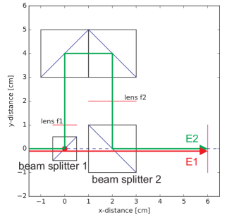
Figure 1: The HOLOCAM in a beam expander setup. The light enters by the left side and is splitted at beam splitter 1 in two beams. One beam ($E1$) passes straightly through the interferometer and hits an imaging plane at the right. The second beam passes by branch 2. Branch 2 contains 2 lenses which can be arranged such as to form a beam expander.

Figure 1 shows an exemplary HOLOCAM device. It consists of a Mach Zehnder type interferometer with two unequal branches. The upper branch (branch 2) is longer and contains, in this example, two lenses. The light enters from the left, is then splitted into two beams and these two beams subsequently come to interference on a screen on the right. The two lightfields are called $E_{1}$, $E_{2}$ being propagated by branch 1,2 respectively.

The intensity $IN$ that is measured on the screen can be expressed as

$$IN(\vec{x}_{s})=\overline{(\vec{E}_{1}(\vec{x}_{s})+\vec{E}_{2}(\vec{x}_{s}))}\cdot(\vec{E}_{1}(\vec{x}_{s})+\vec{E}_{2}(\vec{x}_{s}))$$ (1)

Here and in the following $\cdot$ denotes the scalar product of the field vectors on every pixel. In Equation (1) it is the scalar product between the 3D E-vectors.

$E_{1}(\vec{x}_{s})$,$E_{2}(\vec{x}_{s})$ are the vectorial first and second electric field, respectively. $\vec{x}_{s}$ is the location where the field is measured, s being some index of location, such as an index of a pixel. In Figure 1 the pixel is part of the plane where the fields $E1$ and $E2$ overlap on the right. To simplify the notation, the time variable $t$ (respectively $\omega$) is supressed. The particular meaning should be clear by context. In the following, $\vec{E}_{1}(\vec{x}_{s})$ stands for a quasi monochromatic field with angular frequence $\omega$, yielding $\vec{E}_{1}(t,\vec{x}_{s})=\vec{E}_{1}(\omega,\vec{x}_{s})e^{i\omega t}$. Equation 1 is actually independent of the factor $e^{i\omega t}$. Dropping the vector notation and using the abbreviation $E_{1}(\vec{x}_{s})=:E1_{s}$ Equation 1 becomes

$$IN_{s}=\overline{(E1_{s}+E2_{s})}*{(E1_{s}+E2_{s})}$$ (2)

or

$$IN_{s}=\mid E1_{s}\mid^{2}+\mid E2_{s}\mid^{2}+2\ Re(\ \overline{E2_{s}}*E1_{s}\ )$$ (3)

or further

$$IN=\mid E1\mid^{2}+\mid E2\mid^{2}+2\ Re(\ \overline{E2}*E1\ )$$ (4)

Here and in the following $*$ denotes a point wise multiplication, for instance two pixel vectors $\{x_{s}\}$,$\{y_{s}\}$ are $*$ multiplied to yield a new vector $\{z_{s}\}$ of the same dimension with $x_{s}*y_{s}=z_{s}$ for all pixel indices $s$. ’*’ is essentially different from a scalar product such as ’$\cdot$’ since it does not include summation. In most cases, the indices $s$ enumerate the pixels of the detector. In some cases (such as in Equation (2)) the running pixel index ’s’ is still kept but ’*’ is used. This is actually a redundant expression for the fact that the multiplication is individually performed on every pixel without summation.

Equation (3) is the well known interference expression. $\mid E1_{s}\mid$, $\mid E2_{s}\mid$ are the amplitudes of the electric field from branch 1,2 respectively. These quantities can be measured by conventional methods. Subtracting this background in Equation (3) shows that $Re(\ \overline{E2_{s}}*E1_{s}\ )$ can be measured.

Using known technologies such as ’phase shifting’ or ’carrier phase’ not only $Re(\ \overline{E2_{s}}*E1_{s}\ )$ but the full complex interference term can be measured. This quantity is called IF.

$$IF_{s}=\overline{E2_{s}}*E1_{s}$$ (5)

$IF_{s}$ is a complex field given for all index positions $s$. $IF_{s}$ will be called a hologram in contrast to $IN_{s}$ which is called the inferogram.

In the following, it will be assumed that an appropriately designed interferometer is used. The interferometer should have the property that the set of $\big{\{}E2_{s}\big{\}}$ for all indices $s$ is determined by $\big{\{}E1_{t}\big{\}}$ for all indices t. A simple example for such an interferomter is given in Section IV. Furthermore, the index for polarization will be suppressed. Therefore, polarization effects will be neglected. In many cases this is justified. If needed all equations can be generalized straightforwardly to include explicit polarization. The assumption about the polarization is particularly correct if $E_{1}$ and $E_{2}$ have the same polarization. Then $E_{1}$ becomes a scalar quantity and the ’$\cdot$’ operation in Equation (1) can be suppressed.

Subsequently, a mapping U from fields in branch 1 to fields in branch 2 will be defined.The mapping is defined on the pixels $x_{s}$ of the detector.

$$E2_{s}=\sum_{t}U_{s,t}E1_{t}=:U(E1)=:UE1$$ (6)

For matrices A,B the term A B (without $\cdot$ or $*$ ) stands, as usual, for the matrix multiplication of two matrices. B might be a vector (such as E1) in which case A B stands for the matrix multiplication between A B yielding a new vector. In this case, A stands for a linear mapping (such as U).

The linear mapping U: $E1\rightarrow E2$ in Equation (6) is actually a field propagation. It can be calculated by solving Maxwell’s equations. In the simplest case of a Mach-Zehnder interferometer it represents a back propagation of field E1 from the detection plane given by the locations $\big{\{}x_{t}\big{\}}$ to a plane before the first beam splitter and thereafter a forward propagation from this plane to the detection plane given again by the locations $\big{\{}x_{s}\big{\}}$. The back propagation is along the first branch of the interferometer and the forward propagation is along the second branch of the interferometer. Hence, U is in fact composed of two propagations.

The propagation could obviously show diffraction effects. Moreover, it is possible to choose appropriate focal lengths $f_{1}$, $f_{2}$ in Figure (1) so that U becomes a point mapping.

The mapping U can only be well defined if the Nyquist Shannon criterium is respected. This means that the $\pi$ phase variations of E1, E2 must not be narrower than the $x_{s}$ spacing on the detector.

Care must also be attributed to signal run off through the borders of the representation space $\big{\{}x_{s}\big{\}}$. The run off of signal strength through the borders might well happen in realistic situations. This signal strength does not affect the result though as it is not reflected. The run off of signal strength can be treated physically and numerically exactly. In many cases, it is not too difficult to choose an appropriate design for which U is a well defined physical map. U is usually injective but not necessarily unitary. Examples for U will be given in Section IV.

For the following section, it is important to state that U represents the physical relationship between E1 and E2 and that U is a property of the measuring device. It does not depend on the incoming field. Having sufficient knowledge of the used interferometer U can be calculated even though this might involve some calibration steps. Once these calibration steps have been properly performed the matrix U is determined and fixed for subsequent measurements of unknown fields.

For completeness, it is mentioned that the introduced device is conceived for a certain group of incoming fields. The allowed group of incoming fields is given by an accepted optical field of view and an allowed incoming field diameter. These are characteristics well known from other optical measuring devices. Therefore, the restrictions in the applicability of U are not particular but usual for optical devices.

Under these circumstances the following equation holds

$$IF_{s}=\overline{E2_{s}}*E1_{s}=E1_{s}*\sum_{t}\overline{U_{s,t}E1_{t}}$$ (7)

Whenever needed $E2$ can be expressed by $E1$. As a consequence, Equations (4) and (7) are nonlinear equations for the complex field $E1$. This is normally expressed as an E1 optimization problem falldorf :

$$\left\|IF_{s}-E1_{s}*\sum_{t}\overline{U_{s,t}E1_{t}}\right\|\rightarrow\min$$ (8)

Equation (8) is non linear and probably unstable in the general case.

A new approach is proposed in the following which avoids the convergence problem. For this Equation (7) is multiplied by $\overline{E1_{s}}$ yielding

$$IF_{s}*\overline{E1_{s}}=\mid E1_{s}\mid^{2}\ *\sum_{t}\overline{U_{s,t}}\ \overline{E1_{t}}$$ (9)

$$IF*\overline{E1}=\mid E1\mid^{2}\ *\ \overline{UE1}$$ (10)

In Equation (9) the term $\mid E1\mid^{2}$ can be determined by a conventional intensity measurement. In the following, it is assumed that $\mid E1\mid^{2}$ is already known. Having this pre-knowledge in $\mid E1\mid^{2}$ Equation 9 becomes a linear equation in the unknown complex field $\overline{E1}$.

Taking the conjugate complex of Equation (9) this can be reformulated as an equation for $E1$. Equation (10) is a compact formulation in matrix notation called the ’fundamental equation’ in this context. To the best available knowledge this reformulation of the phase problem has remained unnoticed up to now.

The fundamental Equation (9 , 10 ) represents an exact, simple and linear equation for the complex amplitude of field $E1_{s}$. The measured quantities $\mid E1_{s}\mid^{2}$ and $IF_{s}$ enter the equation as coefficients. The solution space of linear equations is well known. Hence, the difficulties arising from Equation (8) are avoided. In the subsequent sections (Sections III, IV, V), the uniqueness and stability of Equation (10) will be analyzed for properly designed devices.

III Sensitivity of the fundamental equation

For stability analysis a calculation of the functional derivative would be adequate. This is a high dimensional object equivalent to a perturbation expansion as known from quantum mechanics Messiah (1985). The notation of Messiah will be used in the following. The approach allows us to understand the mechanisms responsible for the perturbation (error) propagation.

A perturbation term is introduced in Equation (9) and the new solution is expanded as a function of the perturbation term. The linear operator $H_{0}$ of the unperturbed problem is introduced:

$$0=H_{0}(\overline{E1}):=\mid E1\mid^{2}\ *\ \overline{U}(\overline{E1})-IF*\overline{E1}$$ (11)

The exact solution of the unperturbed problem corresponds to a zero eigenvalue.

Secondly, a perturbed operator H is defined

$$H\overline{E^{p}}:=H_{o}\overline{E^{p}}+\delta IF*\overline{E^{p}}$$ (12)

’p’ stands for perturbed. ${E^{p}}$ can no longer be expected to be an eigenvector to the eigenvalue zero. In fact, some decision has to be made concerning how to define a solution for the perturbed problem. The option chosen here is to look for the adiabatic eigenvector as a function of the perturbation. This is equivalent to looking for the lowest eigenvalue of the perturbed problem Equation (12). Another possible approach would be to find a least square solution of (12). The latter is equivalent to the lowest singular value solution of (12).

$\delta IF$ represents measurement errors in the determination of the hologram $IF$. As $IF$ also $\delta IF$ is an array of complex numbers.

$E1$ denotes an eigenvector of the unperturbed system for the eigenvalue zero. Contrary to quantum mechanics, neither $H_{0}$ nor $\delta IF$ are self adjunct operators. However, without too much loss of generality we assume a non degenerate spectrum of $H_{0}$ and consequently a complete set $\langle n\rvert$, $\lvert n\rangle$ of left and right hand eigenvectors, defined as

$$H_{o}\lvert n\rangle=C_{n}\lvert n\rangle$$ (13)

and

$$\langle n\rvert H_{o}=C_{n}\langle n\rvert$$ (14)

respectively. Normalization is chosen such as

$$\langle m|n\rangle=\delta_{m,n}$$ (15)

and

$$\lVert\lvert n\rangle\rVert=1$$ (16)

holds.

$C_{n}$ are the complex eigenvalues of $H_{0}$.

All vectors are tupels in $s$ - index space of pixels. The bra - vectors $\langle n\rvert$ are not normalized with respect to the complex scalar product $\sum_{s}\overline{a_{s}}b_{s}$ but with respect to the Kronecker product Equation (15).

Using this notation the perturbation theory known from quantum mechanics can be used Messiah (1985). Therefore, an expansion parameter $\lambda$ is introduced which will be set to $\lambda=1$ later.

$$\overline{E1^{p}}(C_{0}+\delta C_{o})=H\overline{E1^{p}}=H_{o}\ \overline{E1^{p}}+\lambda\ \delta IF*\overline{E1^{p}}$$ (17)

and the eigenvalues and eigenvectors become

$$C_{0}+\delta C_{o}=\zeta_{0}+\lambda\zeta_{1}+\lambda^{2}\zeta_{2}+...+\lambda^{n}\zeta_{n}+...$$ (18)

$C_{0}+\delta C_{0}$ is the eigenvalue which evolves from the lowest eigenvalue $C_{0}$ of the unperturbed system. If no other perturbations are present $C_{0}$ and $\zeta_{0}$ equal zero (for the fundamental equation).

$$\overline{E1}+\delta\overline{E1}=\lvert e_{0}\rangle+\lambda\lvert e_{1}\rangle+\lambda^{2}\lvert e_{2}\rangle+...+\lambda^{n}\lvert e_{n}\rangle+...$$ (19)

By definition the relation $\overline{E1}=\lvert e_{0}\rangle$ holds. $\overline{E1^{p}}$ is the eigenvector to the eigenvalue $C_{0}+\delta C_{0}=\delta C_{0}$ of the perturbed problem.

According to MessiahMessiah (1985) the operator $\frac{Q}{a}$ is introduced

$$\frac{Q}{a}=\sum_{n>0}\frac{\lvert n\rangle\langle n\rvert}{C_{0}-C_{n}}$$ (20)

This yields the following iterative solution

$$\zeta_{n}=\langle\overline{E1}\rvert\delta IF\lvert e_{n-1}\rangle$$ (21)

$$\lvert e_{n}\rangle=\frac{Q}{a}\Big{[}(\delta IF-\zeta_{1})\lvert e_{n-1}\rangle-\zeta_{2}\lvert e_{n-2}\rangle-...-\zeta_{n-1}\lvert e_{1}\rangle\Big{]}$$ (22)

In the first order the following formula holds

$$\delta\overline{E1}\doteq\lvert e_{1}\rangle=\frac{Q}{a}\Big{[}(\delta IF-\zeta_{1})*\overline{E1}\Big{]}$$ (23)

Since $\frac{Q}{a}\overline{E1}=0$ by definition this can be further simplified to

$$\delta\overline{E1}\doteq\lvert e_{1}\rangle=\frac{Q}{a}\ (\delta IF*\overline{E1})$$ (24)

Equation (24) is the desired simple small scale formula describing error propagation in the fundamental Equation (10).

In the next two sections (Sections IV to VI) this formalism will be used to study a simple reference case. The error propagation matrix in Formula (24) is still a high dimensional object. Therefore, it is favorable to condense the result to a single key number further. $\delta\overline{E1}$ expresses how much the solution of the perturbed problem deviates from the exact (or ’correct’) solution. Hence, it is appropriate to calculate the standard deviation for $\delta\overline{E1}$. This is the vector norm of $\delta\overline{E1}$ divided by $\sqrt{N_{det}}$, $N_{det}$ being the number of detection points.

The standard deviation is

$$\sigma:=\sqrt{\frac{\sum_{s}\lvert\delta E1_{s}\rvert^{2}}{N_{det}}}=\frac{\lVert\delta\overline{E1}\rVert}{\sqrt{N_{det}}}$$ (25)

The result still depends on the scaling of E1. The reference for the signal strength is the average of E1. Thus, as usual in signal-to-noise figures the expression for the standard deviation (the ’noise’) is divided by the mean signal strength $av(\lvert E1\rvert)$.

$$av(\lvert E1\rvert):=\frac{\sum_{s}\lvert E1_{s}\rvert}{N_{det}}$$ (26)

This yields the following quality (or S/N) parameter called $\sigma_{\delta E1}$:

$$\sigma_{\delta E1}=\frac{\lVert\delta\overline{E1}\rVert}{\sqrt{N_{det}}}\frac{1}{av(\lvert E1\rvert)}$$ (27)

For $\delta IF$ a similar measure can be found:

$$\sigma_{\delta IF}=\frac{\lVert\delta IF\rVert}{\sqrt{N_{det}}}\frac{1}{av(\lvert IF\rvert)}$$ (28)

The following characteristic number for the error propagation in the system can be defined:

$$A_{error}:=\frac{\sigma_{\delta E1}}{\sigma_{\delta IF}}=\frac{\lVert\delta\overline{E1}\rVert}{\lVert\delta\overline{IF}\rVert}\frac{av(\lvert IF\rvert)}{av(\lvert E1\rvert)}$$ (29)

This ratio is called the error amplification factor.

For the phase error a normalized standard deviation can also be defined:

$$\sigma_{\delta\phi_{1}}=\frac{\lVert\delta\phi_{1}\rVert}{\sqrt{N_{det}}}$$ (30)

No reference to the signal size is necessary since the variation of the phase error is always limited by $2\pi$.

There are two possible origins of $\delta IF$, either a, for instance, gaussian random noise source or a projection of the signal IF on a discrete integer space given by the Bit space of the detector. The difference to the unprojected value is the error caused by the detector quantization. For the calculation of the error amplification factor the origin of $\delta IF$ is not of primary importance since every noise source is condensed to a $\sigma_{\delta IF}$. Nevertheless, the process of error generation slightly influences the value $A_{error}$. In the following, the type of noise generation will be noted for numerical results yielding two cases, either gaussian noise or quantization noise.

The following quantity $A\phi_{BIT-error}$ for quantization noise is particularly interesting because it is independent of any normalization:

$$A\phi_{BIT-error}:=\frac{\sigma_{\delta\phi}}{quantization}:=\frac{\lVert\delta\phi_{1}\rVert}{\sqrt{N_{det}}\ 2^{-n_{bit}}}$$ (31)

$n_{bit}$ is the Bit number of the signal IF, i.e. $n_{bit}=10$ means that the signal IF is projected on a 10 Bit number. The difference between the ’exact’ value IF and the projected value is just $\delta IF$.

In the subsequent Section IV, a simple HOLOCAM system will be designed (’the beam expander HOLOCAM’). In the Section VI the error amplification factor $A_{error}$ and the lowest eigenvalue separation $\Delta_{min}C$ will be calculated for the ’the beam expander’ HOLOCAM.

IV Design of a simple HOLOCAM system, the beam expander HOLOCAM

One of the simplest systems to study is a one dimensional system with a Mach Zehnder interferometer (Figure 1). The system could for instance be built using a linear detector array. Hence, the terminus ’one-dimensional’ only concerns the detector. In the second branch, a lens system is installed in such a way that the detector plane self mapped by U becomes a conjugate plane. This means a field point in the detector plane back propagated by branch one and then forward propagated by branch two (including the mapping by the lens system) becomes again a point image in the detector plane. The mapping U is thus a point mapping. An ideal system is assumed neglecting any aberrations in the optical system. If this was not the case the aberrations could be included in U. This is without relevance for the stability analysis though.

The expansion ratio of the beam expander is called $\gamma$ and if not otherwise stated $\gamma=2$ is used. $\gamma=2$ means that the image of the detection plane is expanded by a factor of two.

The point mapping U applied in the discrete pixel space implies some interpolation since the mapping $0,1,2,3..$ to $0,2,4,6,..$ needs to be accomplished by field values of $E2$ at intermediate pixels at $1,3,5,..$. This does not imply any loss of information. Interpolation will be further discussed in Section VII.

A simplification is made by assuming a one dimensional detector array. This systems can actually be built. The detector space not the propagation space is one dimensional. This assumption does not affect the results. Besides, general 2D problems will be studied later on in Section VI.

In the case of 50 detector points and for a selected pixel range from 20 to 30 this could be representetd by the following U matrix:

$$\left[\begin{matrix}0.0&0.0&0.5&0.5&0.0&0.0&0.0&0.0&0.0&0.0\\ 0.0&0.0&0.0&1.0&0.0&0.0&0.0&0.0&0.0&0.0\\ 0.0&0.0&0.0&0.5&0.5&0.0&0.0&0.0&0.0&0.0\\ 0.0&0.0&0.0&0.0&1.0&0.0&0.0&0.0&0.0&0.0\\ 0.0&0.0&0.0&0.0&0.5&0.5&0.0&0.0&0.0&0.0\\ 0.0&0.0&0.0&0.0&0.0&1.0&0.0&0.0&0.0&0.0\\ 0.0&0.0&0.0&0.0&0.0&0.5&0.5&0.0&0.0&0.0\\ 0.0&0.0&0.0&0.0&0.0&0.0&1.0&0.0&0.0&0.0\\ 0.0&0.0&0.0&0.0&0.0&0.0&0.5&0.5&0.0&0.0\\ 0.0&0.0&0.0&0.0&0.0&0.0&0.0&1.0&0.0&0.0\end{matrix}\right]$$ (32)

This is called ’geometric interpolation’, $U_{x}$.

The same kind of interpolation can also be made in Fourier space. Assuming the signal has an upper cup in the size of the Fourier coefficients yields another unambiguous interpolations method. Here, the Fourier representation of the field, which is a continuous function, is evaluated at intermediate points. This interpolation will be called ’Fourier interpolation’ yielding $U_{f}$.

From the preceding, it is obvious that some points are, as a consequence of discretization, calculated by interpolation. Even in this simple case U cannot be represented by a strict point mapping. The latter would be necessary if one wished to take a pointwise logartithm of Equation (5) as done in reference malacara . The error becomes small for very smooth fields with little or no amplitude variation which is not the case for general fields though. Logartithm of Equation (5) is consequently no option for solving the non linear Equation (8).

In the following, the solution of the exact Equation (10) is further analyzed. This is done by introducing random fields for which IF is calculated and for which the original field must then be recovered solving the fundamental Equation (10).

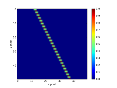
Figure 2: The matrix Ux for the beam expander setup.

Hence, for further analysis a random field $E_{1}$ must be defined.

$$E1(x_{s})=a(\varsigma_{s}+i\ \varrho_{s})$$ (33)

$\varsigma_{s}$,$\varrho_{s}$ being continuous uniform random numbers equally distributed in the half open interval $[-1.0,+1.0)$. ’a’ is a real normalization constant. Adjacent points are absolutely uncorrelated and the phase relation between adjacent points is also random in the range $[-\pi,\pi)$. The unwrapped phase corresponds to a one dimensional random walk with a maximal jump length of $\pi$. This is the maximum variation according to the Nyquist Shannon theorem.

The random field in Equation (33) has by design a flat Fourier spectrum up to the maximum k-vector ($k_{max}=\frac{2\pi}{2\Delta_{pix}}$. $IF$ is a quantity which is in real space a point wise product of $E1$ and $E2$. In order to investigate this influence further $E1$ is not only used in its raw version of Equation (33) but also Fourier filtered by a high frequency cut off in the Fourier spectrum of $E1$. If the cut off is chosen to be for instance $0.5k_{max}$ the input field $E1$ is said to be averaged over two pixel. This is labeled by $n_{av}=2$. $n_{av}=1$ means ’no averaging’. Other magnitudes of averaging are treated analogously.

According to Section III the noise sensitivity of the correct solution is determined by the error amplification factor $A_{error}$, the Bit error amplificationfactor $A\phi_{BIT-error}$ and other quantities definined in Section III.

In the case of the determination of the Bit error ($A\phi_{BIT-error}$) no further random quantity is needed. Otherwise, $\delta IF$ must be defined explicitly by another random field. For this, a gaussian random field with a standard deviation $\sigma_{\delta IF}$ is chosen.

In brief, the terrain is prepared for the numerical runs. As assumed from the beginning the amplitude $\mid E1\mid$ is known from a conventional intensity measurement.

Before doing the actual runs though preconditioning of the fundamental Equation (10) will be discussed in the following section.

V Preconditioning of the fundamental equation

E1 is an eigenvector of the ’exact’ fundamental equation, expressed as $H_{0}$. Due to measurement errors (perturbations) not $H_{0}$ but some $H$ is measured or known. The question is what kind of property of $H$ has to be determined to recover the best approximation of E1 ?

In Section III this has been done by looking for the eigenvector of the lowest eigenvalue. Although this is a valuable strategy it is not necessarily the best one.

Apart from that, Equation (10) can also be solved by minimizing the residual (’least square solution’). This is equivalent to the solution vector for the lowest singular value (’SVD - decomposition’).

The problem of finding a solution of a general homogeneous vector equation $H\overline{E^{p}}=0$ is invariant under left side multiplication by any matrix F, yielding

$$FH\overline{E^{p}}=0$$ (34)

Of course this invariance does not hold for non-zero eigenvalues. Thus, Equation (34) yields different solutions for different preconditioning matrices F. In particular for a perturbed problem (12) the solutions are no longer equivalent. Thus, in case of noise influences different starting points for the solution strategy can be chosen.

Some of the different strategies are mentioned below:

1. $H_{0}:=\mid E1\mid^{2}*\ \overline{U}-IF$

2. $H_{IFn}:=\overline{U}-\mid E1\mid^{-2}*\ IF$

3. $H_{IFU}:=IF^{-1}*\mid E1\mid^{-2}*\ \overline{U}-1$

In particular, a difference is expected for points where $\mid E1\mid$ or $\mid E2\mid$ vanishes or nearly vanishes. If $\mid E1\mid$ or $IF$ is represented in a limited discrete number space on a detector (such as a detector with $n_{bit}$ Bit resolution per pixel) the value of $\mid E1\mid$ or $IF$ attributed to a pixel can become exactly zero. The points where preconditioning is not (or not ’well’) defined can be exempted from preconditioning. This strategy will be applied for all numerical results in this paper.

Of course all different formulations are equivalent for the exact problem (’no noise’).

VI Numerical results for the beam expander HOLOCAM

In a first set of numerical experiments, the error amplification factor $A_{error}$ will be calculated for the expansion ratios $\gamma=2$ and $\gamma=4$. Two solution strategies will be used: either a solution without preconditioning (’pure’) or a solution with IFU preconditioning. In all cases, the eigenvector to the lowest eigenvalue will be determined. The results are calculated for a 14-Bit detector with 1.000 pixels. Hence, quantization is taken as a noise source.

Every data point in the following figures is actually an average over 1.000 runs for different random input fields. Figure (6) shows a histogram of the different results.

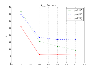
Figure 3: The error amplification factor $A_{error}$ for the beam expander setup, without preconditioning (i.e. ’pure’). The noise source is quantization noise of a 14-Bit detector. $n_{av}$ is the number of pix over which was averaged. $\gamma$ is the expansion ratio of the beam expander in Figure 1. $U_{x}$, $U_{f}$ specifies the propagation matrix.

It can be seen from Figure 3 that, as expected, the error amplification decreases for larger averaging values. $A_{error}$ below $n_{av}=2$ becomes larger as expected from the Nyquist Shannon theorem since these experimental conditions could lead to ambiguous IF values. The results are shown for two different formulations of U: either geometric average in U ($U_{x}$) or Fourier average in U ($U_{f}$). Figures 3,4 represent the results without and with preconditioning, respectively.

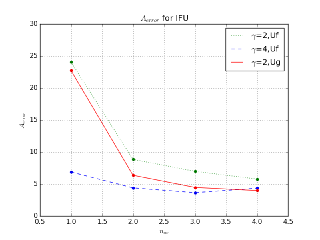
Figure 4: The error amplification factor $A_{error}$ for the beam expander setup using IFU preconditioning (i.e. ’IFU’). The noise source is quantization noise of a 14-Bit detector. $n_{av}$ is the number of pix over which was averaged. $\gamma$ is the expansion ratio of the beam expander in Figure 1. $U_{x}$, $U_{f}$ specifies the propagation matrix.

The results in Figure 4 show that preconditioning can improve the solution stability for certain applications. Moreover, a smaller error amplification is observed for larger $\gamma$ values (as expected).

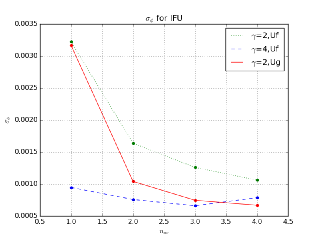
Figure 5: The $\sigma_{\phi}$ variance of the phase determination error for the beam expander setup, using IFU preconditioning (i.e. ’IFU’). The noise source is quantization noise of a 14-Bit detector. $n_{av}$ is the number of pix over which was averaged. $\gamma$ is the expansion ratio of the beam expander in Figure 1. $U_{x}$, $U_{f}$ specifies the propagation matrix.

The phase variance of $1e^{-}3$ corresponds to a factor $A\phi_{BIT-error}$ = 16.3. The variation of the phase signal is $\pm\pi$, hence the phase variance has to be divided by $\pi$ to get a normalized value that can be compared to $A_{error}$. As a result, both values $A\phi_{BIT-error}$ and $A_{error}$ are in reasonable agreement.

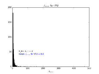
Figure 6: Histogram (1.000 runs) of the error amplification factor $A_{error}$ for the beam expander setup with IFU preconditioning, Uf, $n_{av}=2$, $\gamma=2$. The noise source is quantization noise of a 14-Bit detector.

Figure 6 shows that most runs yield values in a narrow range about E1. Some runs lead to bigger errors. Although the statistical weight of these erroneous data is small they are included in the average of $A_{error}$ (8.8). $A_{error}$ = 3.5 is the factor with the largest statistical weight.

The character of the problem and its solution is further elucidated by the inspection of single run results. A random run with an expansion ratio of $\gamma=2$ and no further averaging ($n_{av}=1$) is chosen, using $U=U_{f}$ .

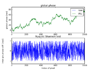
Figure 7: The global phase and the phase difference between adjacent pixels. The upper figure shows the global phase for the unperturbed field $E1$ (’raw’ or ’original’) and the field obtained for the perturbed problem using IFU preconditioning. The global phases are obtained by phase unwrapping. The lower figure represents the phase difference between adjacent pixels for the unperturbed field. The random character can be seen.

Figure 7 shows the initial phase field for the test run. The global phase, as obtained by phase unwrapping, fluctuates in a range of about 80 radians. The phase difference between adjacent pixels is absolutely random, i.e. random in the range $[-\pi,+\pi]$.

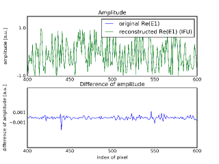
Figure 8: The real part of the complex field E1 for the unperturbed ’raw’ or ’original’ field and the reconstructed field as obtained by solving the fundamental Equation (10). The lower curve shows the difference between the raw field and the reconstructed field. It is plausible that the error is smaller than $1e^{-3}$ rad (for a 14 Bit detector). The restricted range of pixels from 400 to 600 is shown.

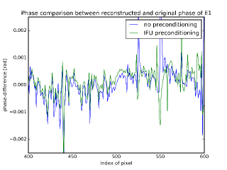
Figure 9: Influence of preconditioning on the reconstruction quality. The restricted range of pixels from 400 to 600 is shown.

Figure 8 depicts the real part of the ’raw’ or ’original’ field and the reconstructed field. For clarity, the lower figure shows the difference between the two fields. In this particular case, there is little difference between ’no preconditioning’ and ’IFU preconditioning’ as shown in Figure (9).

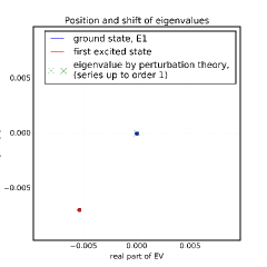
Figure 10: Eigenvalues of the fundamental equation. The lowest eigenvalues of the unperturbed problem and the eigenvalue as obtained by perturbation theory are shown. For 14 Bit quantization noise the perturbed eigenvalue stayed almost immobile at the initial location.

As known from perturbation theory in quantum mechanics, the influence of perturbations on selected eigenstates comes about by the interaction coupling to neighboring states. This arises if the eigenvalues cross as a function of the interaction parameter ($\gamma$). Figure 10 actually shows that such a crossing does not occur. The eigenvalue of first order perturbation theory remains in the neighborhood of the ground state with eigenvalue zero.

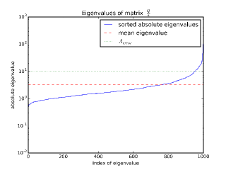
Figure 11: Eigenvalues of the error propagation matrix $\frac{Q}{a}$. The eigenvalues are mainly located in the range 1 to 10. Besides the error propagation factor $A_{error}$ and the mean eigenvalue (for $n_{av}=1$, $\gamma=2$, $U_{f}$, H = ’pure’) are plotted as vertical lines.

Equation (24) gives an explicit expression for the error propagation. As a consequence, the sensitivity is given by the spectrum of eigenvalues of $\frac{Q}{a}$. The explicit calculation results are shown in Figure 11.

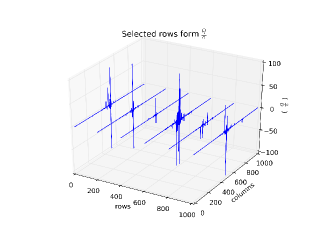
Figure 12: Selected rows of the error propagation matrix $\frac{Q}{a}$. For selected row values all column values are shown.

The structure and explicit matrix values of $\frac{Q}{a}$ can be further analyzed. Selected rows are shown in Figure 12. It can be seen that the matrix has a spiky structure which explains that larger $A_{error}$ values are rarely observed. These larger values still remain in some reasonable neighborhood to the mean value (histogram in Figure 6).

The former analysis is mainly based on a 14 Bit data acquisition. This means that the phase of IF is represented by a 14 Bit integer. Alternatively, the perturbation can be represented by a gaussian noise source as described in Section III. The advantage of this approach is that larger values of $\sigma_{\delta IF}$ can be continuously probed thereby testing the extend of the linear error propagation. This will be done for $\sigma_{\delta IF}$ values from $1e^{-4}$ to $\sigma_{\delta IF}=1$. The latter corresponds to an IF signal that is essentially buried by noise of equal amplitude. No useful phase information is expected to be found for such a noisy situation.

Figure 13 shows an essentially linear relation between the error in $\overline{E1^{p}}$ and the intensity of the noise source. The linear factor $A_{error}$ remains almost constant up to $\sigma_{\delta IF}=0.1$. For higher noise levels, a sublinear behavior is observed. For practical applications it is important not to have a super-linear behavior. The latter would correspond to some kind of ’breakdown’ of the method which is happily not observed.

Furthermore, Figure 14 supports the interpretation of a smooth increase in the deviation of the reconstructed field $\overline{E1^{p}}$ from the unperturbed ’original’ or ’raw’ values. The standard deviation $\sigma_{\delta\phi}$ expresses the degrees of correlation. Figure 14 shows a smooth transition from strongly correlated (small $\sigma_{\delta\phi}$) to uncorrelated. This proves the stability of the HOLOCAM method and is a remarkable result taking into account difficulties in phase reconstruction falldorf .

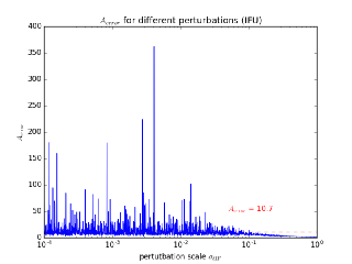
Figure 13: $A_{error}$ for different perturbations $\sigma_{\delta IF}$. $A_{error}$ is constant over almost three order of magnitude. For still higher noise contributions $A_{error}$ decreases.

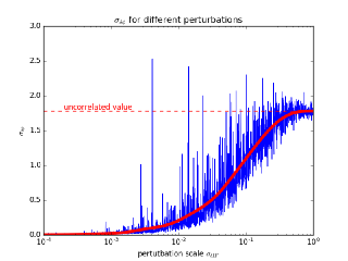
Figure 14: $\sigma_{\delta\phi}$ for different perturbations $\sigma_{\delta IF}$. The figure shows a smooth increase of the phase noise in $\overline{E1^{p}}$. The phase noise saturates as expected at higher noise contributions.

Another important property of the HOLOCAM method is the resolution of $\pi$ phase jumps. To study this property the reconstruction is tested for $E1$ being a standing wave. A 14 Bit detector is used. Figure 15 depicts the ’original’ or ’raw’ field as well as the difference of the reconstructed field compared to the unperturbed ’raw’ field.

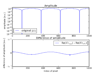
Figure 15: The amplitude of the raw field $E1$ for a standing wave (’log plot’). As expected $|E1|$ becomes zero at some of the pixels. The shown field $E1$ is a standing sine wave which looks unfamiliar since a log scale is used for clarity. The lower figure shows the reconstruction quality by plotting the real difference between the ’raw’ field and the reconstructed field.

The difference between the unperturbed field and the reconstructed perturbed field is further investigated in Figure 16. The upper figure shows an excellent correspondence in the range of $1e^{-3}$ rad. Some spikes are present which are also shown on a larger scale in the lower figure. It can be observed that this spike is half the value of the phase jump ($0.5\pi$). The original ’raw’ field does not have this intermediate phase value. Therefore, this shows up as a spike. Figure 15 shows that this happens at a vanishing amplitude. The difference is not observable for the electrical field (Figure 15).

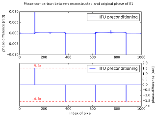
Figure 16: The phase difference beween the raw field and the reconstructed wave. The results are shown on two different scales.

Figure 17 shows the result for the unwrapped phase. Again an almost perfect correspondence between unperturbed ’raw’ fields and reconstructed fields is found. The difference on the right is $2\pi$ which is the intrinsic ambiguity of the phase.

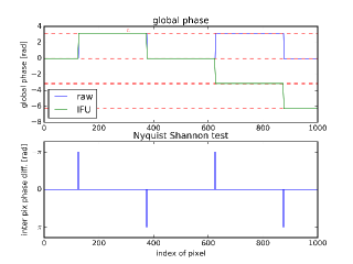
Figure 17: The global phase for the raw field and the reconstructed wave. The right phase jump of the reconstructed field is separated by $2\pi$ from the ’raw’ field. This actually corresponds to the intrinsic $2\pi$ ambiguity of the phase.

Finally, a 2D calculation is shown in Figure 18. No substantial difference between 1D and 2D calculations is found for the E1 field. This might be different for the phase unwrapping step which will not be further investigated here.

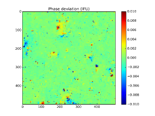
Figure 18: 2D phasemap for a 14 Bit detector for a maximum random field (no correlation between adjacent pixels). Shown is the difference between the original ’raw’ field $E1$ and the reconstructed field $E1^{p}$. The phase noise is essentially in the range $\pm 1e^{-3}$ as in the 1D case. The colorbar shows the phase range $\pm 0.01$ rad.

VII The role of detector quantization

Quantization (or detector quantization) is often the dominant noise source. This is taken into account by choosing an integer representation of the signal on a pixel. A 14 Bit detector means that the signal IF is represented by two 14 Bit integers for the real and the complex part, respectively.

VIII Finite spectral width

Optical fields might have a non negligible spectral width. For this case Equation (10) can be expressed as a frequency dependent equation. Different frequencies separate as shown in Equation (35). The former analysis in Sections II to VI also applies to this case.

$$IF_{\omega}*\overline{E1_{\omega}}=\mid E1_{\omega}\mid^{2}\ *\ \overline{U_{\omega}E1_{\omega}}$$ (35)

IX The role of detector discretization

Discretization expresses the fact that common detectors measure the signal on a rectangular grid of pixels. Every pixel has a finite extension. The signal on a pixel can be assumed to be a weighted average of the incident field intensity on the pixel.

The influence of this pixel averaging can be treated in the framework of the fundamental Equation (10). As a result, the HOLOCAM method can provide the functional value of the electrical field in the center of the pixel. This a remarkable result and another cornerstone for high precision local phase measurements.

It is recalled that the fundamental equation is formulated for a discretization of space which must obey the Nyquist Shannon criterion. In the following, we assume equally spaced grid points ${x_{s,t}}$ on the detector. The Fourier space ${q_{s,t}}$ is introduced. Each Fourier vector is a 2D plane wave on the detector, which is periodic in the boundary conditions. The set of points ${x_{s,t}}$ is finite and so is the set of Fourier vectors ${q_{s,t}}$. The maximum wavevector $q_{max}$ in ${q_{s,t}}$ is $q_{max}=\pi/\Delta_{pix}$, $\Delta_{pix}$ being the pixel spacing. The Nyquist Shannon criterium states that the maximum wavevector $qE1_{max}$ found in the electrical field $E1$ must not exceed the maximum wavevector $q_{max}$. The quantity $qE1_{max}$ is a property of the field $E1$. It is defined independently of the detector or pixel size. The same analysis holds for $E2$ and $IF$. $qE2_{max}$ and $qIF_{max}$ are defined analogously. The maximum of these three field wavevectors is called $qF_{max}$ and $qF_{max}$ must be smaller than $q_{max}$.

The electrical fields $E1$,$E2$ as well as $IF$ are continuously differentiable. By choosing a support large enough the field IF can be expressed as

$$IF(x)=\sum_{q\in\{q_{s,t}\}}^{q_{max}}\hat{IF}(q)e^{-iqx}$$ (36)

The support is chosen such that $IF=0$ and $\nabla IF=0$ holds on the border of the support ($\nabla$ is the gradient on the border). The field IF therefore fulfills periodic boundary conditions. The summation is performed over a finite number of terms. According to Fourier theory the Fourier expansion converges point wise to the fields. At first glance, this applies only to the grid values ${x_{s,t}}$. But the same question can be asked for arbitrary points x, i.e. not necessarily at a grid point.

It is remarkable that Equation (36) holds on every point of the continuous support, not only on the discrete points, assumed that the function IF satisfies periodic boundary conditions and the Nyquist Shannon condition is respected. Choosing a sufficiently large detector size and a sufficiently fine spaced detector this assumption can in fact be fulfilled.

This can be proven as follows: Testing spatial points not given by the grid ${x_{s,t}}$ is equivalent to the introduction of higher q values in the expansion of Equation (36). The points become regular points of the reciprocal lattice to these higher q values. The convergence of the Fourier expansion is again point wise but the new points are included. Thus, the Fourier expansion has the correct function value at the newly introduced spatial points. According to the assumption, the Fourier amplitudes of the newly introduced higher q modes are zero. Consequently, the functional values for these off grid points are just given by the unchanged Equation (36).

It is the purpose of the measurement process to determine the amplitudes $\hat{IF}(q)$ or $IF(x)$ in Equation (36). The Fourier transform yields

$$\hat{IF}(q)=\frac{1}{\mu_{sup}}\sum_{x_{i}}^{support}IF(x_{i})e^{iqx_{i}}$$ (37)

Here and in the following index $i$ denotes an index tupel $i=\{s,t\}$. $\mu_{sup}$ is some normalization constant depending on the support of the Fourier expansion. The difficulty with this formula is that $IF(x_{i})$ is actually unknown.

Only the pixel averaged quantities are known:

$$<IF>(x_{i})=\int_{A_{i}}IF(x)dx$$ (38)

$A_{i}$ being the surface of pixel $x_{i}$.

The quantities actually measured are $<IF>(x_{i})$ and $\hat{<IF>}(q)$, with

$$<IF>(x_{i})=:\frac{1}{\mu_{sup}}\sum_{x_{i}}^{support}\hat{<IF>}(q)e^{-iqx_{i}}$$ (39)

Inserting Equation (36) in Equation (38) yields

$$<IF>(x_{i})=\sum_{q}^{q_{max}}\hat{IF}(q)\int_{A_{i}}e^{-iqx}dx$$ (40)

which can be inverted yielding $\hat{IF}(q)$. Using the inverse Fourier transform yields the value sought ($IF(x_{i})$). Hence, the problem of finding the non-averaged IF values on a grid can be solved in principle.

To give an example $\int_{A_{i}}e^{-iqx}dx$ is evaluated with an $A_{i}$-size of $\Delta_{pix}$. It yields

$$\int_{A_{i}}e^{-iqx}dx=a\ e^{-iqx_{i}}\ sinc(q/q_{max})$$ (41)

a being some normalization constant. Equation (40) can be rewritten as

$$<IF>(x_{i})=a\ \sum_{q}^{q_{max}}\hat{IF}(q)sinc(q/q_{max})e^{-iqx_{i}}\$$ (42)

This is the Fourier expansion for the averaged values. The expansion coefficients are unique. As a result, comparing coefficients with Equation (39) yields

$$\hat{<IF>}(q)=\hat{IF}(q)sinc(q/q_{max})$$ (43)

As expected, the non averaged quantities $\hat{IF}(q)$ are determined by the averaged quantities $<\hat{IF}>(q)$. The relationship is a multiplication in q-space. The inverse function is needed leading from the averaged values to the non averaged values. This corresponds to a folding in x-space. The kernel for this folding in real space is called K. K must be folded with the measured averaged data to get the point data in demand in the center of the pixel.

$$K(x)=K_{0}\int_{|q|<q_{max}}\frac{1}{sinc(q/q_{max})}e^{-iqx}dq$$ (44)

The sum $\sum$ has been replaced by an integral, $K_{0}$ being a normalization constant, $q<q_{max}$. Expanding the 1/sinc function in terms of $q/q_{max}$ yields the following approximation:

$$K(x)\approx K_{0}\int_{q_{max}}^{q_{max}}[1+(q/q_{max})^{2}/3!]e^{iqx}dq$$ (45)

or introducing $n_{g}=\frac{x}{\Delta_{pix}}$, $n_{g}$ being the separation in units of $\Delta_{pix}$ (’g’ stands for grating).

$$K(n_{g}{\Delta_{pix}})\approx K_{0}\int_{-1}^{1}[1+y^{2}/3!]e^{i\pi yn_{g}}dy$$ (46)

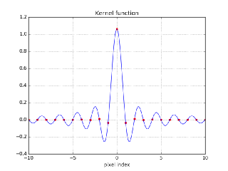
Figure 19: Kernel for the inverse filtering from averaged pixel values to point values.

The integral can be calculated analytically. The kernel function is plotted in Figure (19). For the inverse folding operation only integer values $n_{g}$ are needed.

$$\sum_{i}<IF>(x_{i})K(x_{j}-x_{i})=IF(x_{j})$$ (47)

Thus, Equation (47) calculates, as intended, the point values of IF out of the measured averages $<IF>(x_{i})$. The averaging effect of the detector can be treated correctly in Equation 10. This is another important cornerstone for high precision field measurements.

X A preview on entangled light detection

The HOLOCAM detection principle is based on space resolved correlations. This can also be used to analyze non classical light properties. The incoming quantum mechanical light state is called $\Psi$. To be specific a non-classical two photon state (or Bi-photon state) is assumed. This includes two photon number states and two photon coherent vacuum states (squeezed vacuum states). In the Heisenberg picture these states have a double frequency dependence of the generating operator. The squeezing operator is given by Loudon (2010):

$$\hat{S_{0}}(\zeta_{s})=exp({0.5(\ \bar{\zeta_{s}}\hat{a}_{s}^{2}+\zeta_{s}(\hat{a}_{s}^{\dagger})^{2})})$$ (48)

(s is some arbitrary pixel index, 0 expresses the time independence)

In the Heisenberg picture the operator time dependence becomes:

$$\hat{S(t)}(\zeta)=\hat{S_{0}}(\ \zeta\ e^{2i\omega t})$$ (49)

This time dependence corresponds to a doubled k vector of the Bi-photon in the Schrödinger picture. The Bi-photon $\Psi$ has a 2 fold space dependence $\Psi(x_{2},x_{1})$, $x_{1}$,$x_{2}$ being the coordinate of the first and the second photon, respectively. According to Bose statistics the function is symmetric upon permutation of the ordering. On the light path the phase changes as $\Psi\rightarrow\Psi e^{2ik\delta l}$.

According to quantum optics Loudon (2010) this light state is split into three components by a beam splitter. Light states where both wave parts follow path 1 or path 2 and a third option which only exists in quantum mechanics where 1 photon passes by path 1 and 1 photon passes by path 2. These three wave functions are called $\Psi_{20}$, $\Psi_{02}$, $\Psi_{11}$. The experimental situation discussed corresponds to the setup in Figure 1.

On the detector, a superposition of these three wave functions is formed. This step of superposition must be done carefully since further wave components are generated on the second beam splitter. The effects on beam splitter 1 and beam splitter 2 are quite similar. In the experiment described here, only the states where both photons reach the detector are of interest. Other states should be ideally rejected.

Different solutions exist to this problem. It is the conceptually simplest approach to limit oneself to two photon number states and to use a two photon detector Loudon (2010). Thus, this is chosen here. As a consequence, Bi-photon splitting on the second beam splitter will be neglected and the following interference signal QIN is measured:

$$QIN_{s}=\langle\Psi_{20}+\Psi_{02}+\Psi_{11}\rvert N(x_{s})\lvert\Psi_{20}+\Psi_{02}+\Psi_{11}\rangle$$ (50)

$N(x_{s})$ is the 2 photon number operator ($(\hat{a}_{s}^{\dagger})^{2}(\hat{a}_{s})^{2}$) representing the detector pixel $x_{s}$. To some extent QIN replaces the previously introduced quantity IN (Section II) although differences exist.

As usual in interference experiments, the double sum in Equation (50) can be multiplied out yielding intensity and interference terms.

There is only one term (and its conjugate complex) which has a Bi-photon path length dependence such as in Equation (49).

$$QIN_{s}=\langle\Psi_{20}\rvert N\lvert\Psi_{02}\rangle e^{2ik\delta l}+c.c.+^{\prime}otherterms^{\prime}$$ (51)

’other terms’ designates terms which do not have the ’double k’ dependence on path variations $\delta l$ in the interferometer.

Hence, using a phase resolving method, such as phase shifting, $\langle\Psi_{20}\rvert N(x_{s})\lvert\Psi_{02}\rangle$ and furthermore $\langle\Psi_{20}\rvert N(x_{s})\lvert\Psi_{20}\rangle$ and $\langle\Psi_{02}\rvert N(x_{s})\lvert\Psi_{02}\rangle$ can be measured.

The space index in $N(x_{s})$ indicates that every pixel is measured. The methods have already been used for Equation (4).

Knowing the detector response Loudon (2010) yields the quantity

$$QIF_{s,s}=\overline{\Psi 2_{s,s}}\Psi 1_{s,s}$$ (52)

and similarly the quantities $|\Psi 2_{s,s}|^{2}$ and $|\Psi 1_{s,s}|^{2}$. The short notation $\Psi 1_{s,s}$, $\Psi 2_{s,s}$ has been introduced for $\Psi_{20}(x_{s},x_{s})$, $\Psi_{02}(x_{s},x_{s})$ respectively. The equation holds for equal values in the x-entry slots of $\Psi_{20}(x_{s},x_{s})$. The double index with identical values indicates that the quantity denotes properties of the Bi-photon field for one and the same index.

The measuring device comprises a first beam splitter, two arms which are again described by some single mode propagation matrix U (Section II). As in Section IV an appropriate interferometer with a point mapping U is assumed (Figure 1). Following the rules of Section IV a mapping of the Bi-photon in branch 1 called $\Psi 1_{s,t}$ to branch 2 can be derived.

$$\Psi 2_{s,t}=\sum_{s,t}U^{\diamond}_{s,t,m,n}\Psi 1_{m,n}=U^{\diamond}(\Psi 1)$$ (53)

In general, this mapping is a linear function of the array of indices $(s,t),(m,n)$. In the case of a point mapping though $U^{\diamond}$ maps diagonal (s,s) matrix elements on diagonal (m,m) elements. The mapping is essentially ’geometric’ and there is no smearing out by diffraction.

$$\Psi 2_{s,s}=\sum_{s}U^{\diamond}_{s,s,m,m}\Psi 1_{m,m}=\sum_{s}U_{s,m}^{2}\Psi 1_{m,m}$$ (54)

$U_{s,m}^{2}$ denotes the square of the U matrix element in Equation 6. Thus, this is a simple rule to deduce $U^{\diamond}$ from $U$.

An equation similar to Equation (7) holds

$$QIF_{s,s}=\overline{\Psi 2_{s,s}}\Psi 1_{s,s}=\Psi 1_{s,s}\sum_{t}\overline{U_{s,s,t,t}^{\diamond}\Psi 1_{t,t}}$$ (55)

The solution is identical to Equation (7). $\Psi 1_{s,s}$ denotes the complex field value of the Bi-photon state on index $(s,s)$, s denoting for instance a pixel on the detector.

It should be mentioned that $\langle\Psi_{11}\rvert N\lvert\Psi_{02}\rangle e^{ik\delta l}$ and $\langle\Psi_{11}\rvert N\lvert\Psi_{20}\rangle e^{ik\delta l}$ potentially allow to measure ’off-diagonal’ (s,t) states of $\Psi 1(s,t)$. The measured quantities are of the type $\Psi_{20}(s,s)\Psi_{11}(s,s)$, $\Psi_{02}(s,s)\Psi_{11}(s,s)$. For this step $\Psi_{20}(s,s)$ and $\Psi_{02}(s,s)$ must be known from the first procedure. The involved equations can be directly solved yielding $\Psi_{11}(s,s)$. Using the properties of U and the mapping of $\Psi_{11}(s,s)$ similar to Equation (54) a set of off-diagonal elements of $\Psi 1(s,t)$ can be measured. By shearing the two paths of the interferometer other index combinations can be measured.

This shows that a careful combination of HOLOCAM and shearing methodology allows us to measure the hole set of general Bi-photon parameters $\Psi 1(x_{2},x_{1})$.

The Bi-photon HOLOCAM should be useful for super resolution microscopy and cutting edge metrology. The information is different from homodyne detection. This can be immediately concluded from the fact that the Bi-photon states (such as the Bi-photon number states) used in Chapter X have vanishing electrical field expectation values. Nevertheless, the Bi-photon HOLOCAM can measure their wave functions.

References

- Yoshizawa Ed. (2015) T. Yoshizawa Editor, Handbook of optical metrology, 2nd ed. (CRC Press, Boca Raton, 2015)
- Born and Wolf (1991) M. Born and E. Wolf, Principles of optics, 6th ed. (Pergamon Press, Oxford, 1991)
- (3) C.Falldorf, A.Simic, C. von Kopylow, R.B.Bergmann, Computational Shear Interferometry: A versatile toll for wave field sensing, Imaging and Applied Optics OSA Technical Digest (online) (Optical Society of America, 2013), paper JW2B.3 https://doi.org/10.1364/AIO.2013.JW2B.3
- Rhoadarmer (2004) T.A. Rhoadarmer, Development of a self-referencing interferometer wavefront sensor, Proc. SPIE 5553, Advanced Wavefront Control: Methods, Devices, and Applications II, 112 ( 2004)
- (5) W. J. Wild and E. O. Le Bigot, Development of a self-referencing interferometer wavefront sensor, “Rapid and robust detection of branch points from wave-front gradients, ”Optics Letters 24, pp. 190–192, Feb. 1999.
- (6) Daniel Malacara editor, Optical Shop Testing 3rd Edition, “John Wiley & Sons, 2007.
- Messiah (1985) A. Messiah, Quantenmechanic, 2nd ed. (Walter de Gruyter, Berlin New York, 1985)
- Loudon (2010) R. Loudon , The Quantum Theory of Light, 3rd ed. (Oxforf science Publications, Oxford , 2010)