Estimation and Inference for Very Large Linear Mixed Effects Models

Abstract

Linear mixed models with large imbalanced crossed random effects structures pose severe computational problems for maximum likelihood estimation and for Bayesian analysis. The costs can grow as fast as $N^{3/2}$ when there are $N$ observations. Such problems arise in any setting where the underlying factors satisfy a many to many relationship (instead of a nested one) and in electronic commerce applications, the $N$ can be quite large. Methods that do not account for the correlation structure can greatly underestimate uncertainty. We propose a method of moments approach that takes account of the correlation structure and that can be computed at $O(N)$ cost. The method of moments is very amenable to parallel computation and it does not require parametric distributional assumptions, tuning parameters or convergence diagnostics. For the regression coefficients, we give conditions for consistency and asymptotic normality as well as a consistent variance estimate. For the variance components, we give conditions for consistency and we use consistent estimates of a mildly conservative variance estimate. All of these computations can be done in $O(N)$ work. We illustrate the algorithm with some data from Stitch Fix where the crossed random effects correspond to clients and items.

and

t1Supported under US NSF Grant DGE-114747 t2Supported under US NSF Grant DMS-1407397

1 Introduction

The field of statistics is confronting two important challenges at present. The first is the arrival of ever larger data sets, sometimes described as ‘big data’. See, for instance, Provost and Fawcett, (2013) and Varian, (2014). The second is the reproducibility crisis, in which published findings cannot be replicated. This problem was clearly presented by Ioannidis, (2005) among others, and it has lead to the American Statistical Association releasing a statement on $p$-values (Wasserstein and Lazar,, 2016).

We might naively hope that the first problem would remove the second one. While larger data sets can greatly reduce uncertainty, difficulties remain. The one that we consider here is a crossed random effects structure in the data. That structure introduces a dense tangle of correlations that can sharply reduce the effective sample size of the data at hand. If, as we suspect, most data scientists treat these large data sets as IID samples, then they will greatly underestimate the uncertainty in their fitted models. The usual methods for this problem, whether based on maximum likelihood or on Bayes, scale badly to large data sets, with a cost that grows superlinearly in the sample size. We present and study a method of moments approach with cost that scales linearly in the problem size, among other advantages.

The sort of data that motivate us arise in e-commerce applications. The factors are variables like cookies, customer IDs, query strings, IP addresses, product IDs (e.g., SKUs), URLs and so on. The most direct way to handle such variables is to treat them as categorical variables that simply happen to have a large number of levels, including many that have not yet appeared in the data. We think that a random effects model is more appropriate. For instance, internet cookies are cleared regularly and hence any specific cookie is likely to disappear shortly. It is therefore appropriate to consider the specific cookies in a data set as a sample from some distribution, that is, as a random effect. Similarly there is turnover in popular products and queries, that motivate treating them as random effects too.

While the largest crossed random effect data sets we know of are in e-commerce, we expect the problem to arise in other settings where data set sizes are growing. The crossed random effects structure is very fundamental. Any setting with a many to many mapping of factor levels involves crossed effects that one might want to model as random. In agriculture there are gene by environment crosses. In education, neither schools nor neighborhoods are perfectly nested within the other (Raudenbush,, 1993) and in multiyear data sets there is a many to many relationship between teachers and students.

When our chosen model involves only one of these random effect entities then a hierarchical model, based on Bayes or empirical Bayes, can be quite effective. Things change considerably when we want to use two or more crossed random effects. In this paper, we consider the following model,

Model 1.

Two-factor linear mixed effects:

$$\begin{split}&Y_{ij}=x_{ij}^{\mathsf{T}}\beta+a_{i}+b_{j}+e_{ij},\quad x_{ij}\in\mathbb{R}^{p},\quad i,j\in\mathbb{N}\quad\text{where},\\ &a_{i}\stackrel{{\scriptstyle\mathrm{iid}}}{{\sim}}(0,\sigma^{2}_{A}),\quad b_{j}\stackrel{{\scriptstyle\mathrm{iid}}}{{\sim}}(0,\sigma^{2}_{B}),\quad e_{ij}\stackrel{{\scriptstyle\mathrm{iid}}}{{\sim}}(0,\sigma^{2}_{E})\quad\text{(independently) and},\\ &\mathbb{E}(a_{i}^{4})<\infty,\quad\mathbb{E}(b_{j}^{4})<\infty,\quad\mathbb{E}(e_{ij}^{4})<\infty.\end{split}$$ (1)

For instance, customer $i$ might assign a score $Y_{ij}$ to product $j$. Then $x_{ij}$ contains features about the customer or product or some joint properties of them, $\beta$ is of interest for the company choosing what product to recommend, $b_{j}$ measures some general appeal of the product not captured by the features in $x_{ij}$, while $a_{i}$ captures variation in which customers are harder or easier to please and $e_{ij}$ is an error term. This is a mixed effects model because it contains both random effects $a_{i}$, $b_{j}$ and fixed effects $x_{ij}$.

Model 1 describes any $ij$ pair, but the given data set will only contain some finite number $N$ of them. If the available data are laid out as rows $i$ and columns $j$ with $R$ distinct rows and $C$ distinct columns, then the cost of fitting a generalized least squares regression model for $\beta$ scales as $O((R+C)^{3})$ because it solves a $p\times p$ system of equations with $p\geqslant R+C$. See Searle et al., (1992), Raudenbush, (1993) and Bates, (2014). Now because $RC\geqslant N$ we have $\max(R,C)\geqslant\sqrt{N}$ and $(R+C)^{3}>N^{3/2}$.

Gao and Owen, (2017) consider an intercept-only version of Model 1 where $x_{ij}^{\mathsf{T}}\beta$ is simply a constant $\mu\in\mathbb{R}$ for all $i$ and $j$. They find that Markov chain Monte Carlo does not solve the inference problem. All of the MCMC methods considered either failed to mix, or converged to the wrong answer, and this took place already at modest sample sizes. For the specific case of a Gibbs sampler and Gaussian $a_{i}$, $b_{j}$ and $e_{ij}$, using methods from Roberts and Sahu, (1997) they show it will take $O(N^{1/2})$ iterations costing $O(N)$ each to converge, for a total cost of $O(N^{3/2})$. Fox, (2013) presents a very general equivalence between the convergence rate of an iterative equation solver and the convergence rate of an associated MCMC scheme, so these identical rates may be a sign of a deeper equivalence. Consensus Bayes (Scott et al.,, 2016) splits the data into shards, one per processor. However the data given to each shard has to be independent and here data sets corresponding to a subset of rows will have correlations due to commonly sampled columns (and vice versa).

We find that existing Bayes and likelihood methods are not effective for this problem. Here we present an approach based on the method of moments. We seek estimates $\hat{\beta}$, $\hat{\sigma}^{2}_{A}$, $\hat{\sigma}^{2}_{B}$ and $\hat{\sigma}^{2}_{E}$ along with variance estimates for these quantities. We have three criteria:

1. the total computational cost must be $O(N)$ time and $O(R+C)$ space,

2. the variance estimates should be reliable or conservative, and

3. we prefer $\hat{\beta}$ to be statistically efficient.

We regard the first criterion as a constraint that must be met. For the second criterion, a mild over-estimate of $\mathrm{Var}(\hat{\beta})$ is acceptable in order to keep the costs in $O(N)$. The third criterion is to be met as well as we can, subject to constraints given by the first two. Computational efficiency is more important than statistical efficiency in this context. For very large $N$, requiring $O(N^{3/2})$ computation is like asking for an oracle.

The method of moments meets our $O(N)$ time and $O(R+C)$ space criteria, and here we show that it can also yield reliable variance estimates. Further advantages of the method of moments are that it does not require parametric distributional assumptions, there are no tuning parameters to choose, and most importantly for large $N$, it is very well suited to parallel computation. The method of moments is not without drawbacks. Sometimes it yields parameter estimates that are out of bounds, such as negative variance estimates.

An outline of this paper is as follows. Section 2 introduces most of the notation for Model 1, especially the pattern of missingness in the data, and gives some of the asymptotic assumptions. Section 3 presents our algorithm and shows that it takes $O(N)$ time and $O(R+C)$ space. We compute a generalized least squares (GLS) estimate for a model with either row or column variance components, but not both. We choose based on an efficiency criterion. Then we estimate $\mathrm{Var}(\hat{\beta})$ accounting for all three error terms including the one left out of the GLS estimate. Section 4 illustrates our algorithm with some ratings data from Stitch Fix. There $Y_{ij}$ is a rating, from a $10$ point scale, by customer $i$ on item $j$, with features $x_{ij}$. Compared to OLS estimates, the random effects model leads to standard errors on coefficients $\beta_{j}$ that can be more than ten times higher. That may be interpreted as an effective sample size which is less than $1$% of the nominal sample size. Section 5 gives conditions under which $\hat{\beta}\stackrel{{\scriptstyle p}}{{\to}}\beta$, and further conditions for the variance components to be consistent. There is also a central limit theorem for $\hat{\beta}$. Section 6 compares our method of moments estimator to a state of the art GLMM code (Bates,, 2016) written in Julia (Bezanson et al.,, 2017). We find that algorithm takes $O(N^{3/2})$ cost per iteration, with a number of iterations that, in our simulations, depends on $N$. On problems where the GLMM code gives an answer we find it more statistically efficient for $\beta$ and $\sigma^{2}_{E}$ but not for $\sigma^{2}_{A}$ or $\sigma^{2}_{B}$. Section 7 discusses some future work.

Our method of moments approach is similar to methods Henderson, (1953) develops for Gaussian data. Gao and Owen, (2017) use $U$-statistics to find a counterpart to the Henderson I estimator that can be computed in $O(N)$ time and $O(R+C)$ space. They also get a variance estimator for their variance components, without assuming a Gaussian distribution. The variance estimator can be computed in $O(N)$ time. It targets a mildly conservative upper bound on the variance as the variance itself, like the one for Henderson’s estimates, takes more than $O(N)$ computation. In this paper we incorporate fixed effects along with the random effects, just as Henderson II does in generalizing Henderson I. Henderson III allows for interactions between fixed and random effects. We believe such interactions are very reasonable in our motivating applications, but incorporating them is outside the scope of this article.

Our analysis is for a fixed dimension $p$. This is reasonable for our motivating data from Stitch Fix, where $p\ll N$. It remains to develop methods for cases where $p\to\infty$ with $N$.

Another issue that we do not address in this article is selection bias in the available observations. Sometimes ratings are biased towards the high end because customers seek products that they expect to like and companies endeavor to recommend such products. In other data sets, such as restaurant reviews, customers may be more likely to make a rating when they are either very unhappy or very happy. For such data, the ratings will be biased towards both extremes and away from the middle. Accounting for selection bias requires assumptions or information from outside the given data. Propensity weighting (Imbens and Rubin,, 2015, Chapter 13) could well fit into our framework, but we leave that out of this paper, as the basic problem without selection bias is already a challenge.

2 Notation and asymptotic conditions

Here we give a fuller presentation of our notation. Equation (1) describes the distribution of seen and future data. We call the first index of $Y_{ij}$ the ‘row’ and the second the ‘column’. We use integers $i,i^{\prime},r,r^{\prime}$ to index rows and $j,j^{\prime},s,s^{\prime}$ for columns, but the actual indices may be URLs, customer IDs, or query strings. The index sets are countably infinite to always leave room for unseen levels in the future.

The variable $Z_{ij}$ takes the value $1$ if $(x_{ij},Y_{ij})$ is observed and $0$ otherwise. We assume that there is at most one observation in position $(i,j)$. For customer rating data, we suppose that if $i$ has rated $j$ multiple times, then only the most recent rating is retained. In many other settings, only a negligible fraction of $ij$ pairs will have been duplicated.

The sample size is $N=\sum_{ij}Z_{ij}<\infty$. The number of observations in row $i$ is $N_{i\text{\tiny$\bullet$}}=\sum_{j}Z_{ij}$ and the number in column $j$ is $N_{\text{\tiny$\bullet$}j}=\sum_{i}Z_{ij}$. The number of distinct rows is $R=\sum_{i}1_{N_{i\text{\tiny$\bullet$}}>0}$ and there are $C=\sum_{j}1_{N_{\text{\tiny$\bullet$}j}>0}$ distinct columns. In the following, summing over rows $i$ means summing over just the $R$ rows $i$ with $N_{i\text{\tiny$\bullet$}}>0$, and similarly for sums over columns. This convention corresponds to what happens when one makes a pass through the whole data set.

Let $Z$ be the matrix containing $Z_{ij}$. Then $(ZZ^{\mathsf{T}})_{ii^{\prime}}=\sum_{j}Z_{ij}Z_{i^{\prime}j}$ is the number of columns for which we have data in both rows $i$ and $i^{\prime}$. Similarly, $(Z^{\mathsf{T}}Z)_{jj^{\prime}}$ is the number of rows in which both columns $j$ and $j^{\prime}$ are observed. Note that $(ZZ^{\mathsf{T}})_{ii^{\prime}}\leqslant N_{i\text{\tiny$\bullet$}}$ and $(Z^{\mathsf{T}}Z)_{jj^{\prime}}\leqslant N_{\text{\tiny$\bullet$}j}$. We will use the following identities:

$$\sum_{ir}(ZZ^{\mathsf{T}})_{ir}=\sum_{j}N_{\text{\tiny$\bullet$}j}^{2},\quad\text{and}\quad\sum_{js}(Z^{\mathsf{T}}Z)_{js}=\sum_{i}N_{i\text{\tiny$\bullet$}}^{2}.$$

This notation allows for an arbitrary pattern of observations. We mention three special cases. A balanced crossed design has $Z_{ij}=1_{i\leqslant R}1_{j\leqslant C}$. If $\max_{i}N_{i\text{\tiny$\bullet$}}=1$ but $\max_{j}N_{\text{\tiny$\bullet$}j}>1$ then the data have a hierarchical structure with rows nested in columns. If $\max_{i}N_{i\text{\tiny$\bullet$}}=\max_{j}N_{\text{\tiny$\bullet$}j}=1$, then the observed $Y_{ij}$ have IID errors. Some of these patterns cause problems for parameter estimation. For example, if the errors are IID, then the variance components are not identifiable. Our assumptions rule these out to focus on large genuinely crossed data sets.

The following vectors are useful for subsequent analyses. Let $v_{1,i}$ be the length-$N$ vector with ones in entries $\sum_{r=1}^{i-1}N_{r\text{\tiny$\bullet$}}+1$ to $\sum_{r=1}^{i}N_{r\text{\tiny$\bullet$}}$ and zeros elsewhere. Similarly, let $v_{2,j}$ be the length-$N$ vector with ones in entries $\sum_{s=1}^{j-1}N_{\text{\tiny$\bullet$}s}+1$ to $\sum_{s=1}^{j}N_{\text{\tiny$\bullet$}s}$ and zeros elsewhere.

Next, we describe our asymptotic assumptions. First

$$\epsilon_{R}=\max_{i}N_{i\text{\tiny$\bullet$}}/N\to 0,\quad\text{and}\quad\epsilon_{C}=\max_{j}N_{\text{\tiny$\bullet$}j}/N\to 0,$$ (2)

so no single row or column dominates. The average row size can be measured by $N/R$ or by $\sum_{i}N_{i\text{\tiny$\bullet$}}^{2}/N$; the latter is $\mathbb{E}(N_{i\text{\tiny$\bullet$}})$ when choosing one of the $N$ data points $(i,j,x_{ij},Y_{ij})$ at random (uniformly). Similar formulas hold for the average column size. These average row and column sizes are $o(N)$, because

$$\frac{1}{N^{2}}\sum_{i}N_{i\text{\tiny$\bullet$}}^{2}\leqslant\epsilon_{R}\to 0,\quad\text{and}\quad\frac{1}{N^{2}}\sum_{j}N_{\text{\tiny$\bullet$}j}^{2}\leqslant\epsilon_{C}\to 0.$$

We often expect the average row and column sizes, while growing slower than $N$, should diverge:

$$\min(N/R,N/C)\to\infty,\quad\text{and}$$

$$\begin{split}&\min\Bigl{(}\frac{1}{N}\sum_{i}N_{i\text{\tiny$\bullet$}}^{2},\frac{1}{N}\sum_{j}N_{\text{\tiny$\bullet$}j}^{2}\Bigr{)}\to\infty.\end{split}$$

We do not however impose these conditions.

Even for large average row and columns sizes, there can still be numerous new or rare entities with $N_{i\text{\tiny$\bullet$}}=1$ or $N_{\text{\tiny$\bullet$}j}=1$. Our analysis can include such small rows and columns without requiring that they be deleted. When there are covariates $x_{ij}$ we need to rule out degenerate settings where the sample variance of $x_{ij}$ does not grow with $N$ or where it is dominated by a handful of observations. We add some such conditions when we discuss central limit theorems in Section 5.2.

The finite fourth moments $\mathbb{E}(a_{i}^{4})$, $\mathbb{E}(b_{j}^{4})$ and $\mathbb{E}(e_{ij}^{4})$ are conveniently described through finite kurtoses $\kappa_{A}$, $\kappa_{B}$ and $\kappa_{E}$, respectively. Some of the variance expressions in Gao and Owen, (2017) are dominated by terms proportional to $\kappa+2$ for one of these kurtoses. Following Gao and Owen, (2017) we assume that $\min(\kappa_{A},\kappa_{B},\kappa_{E})>-2$. This lower bound rules out some symmetric binary distributions for $a_{i}$, $b_{j}$ and $e_{ij}$. Such cases seem unrealistic for our motivating applications.

The randomness in $Y_{ij}$ comes from $a_{i}$, $b_{j}$ and $e_{ij}$. In some places we combine them into $\eta_{ij}\equiv a_{i}+b_{j}+e_{ij}$.

Gao and Owen, (2017) found exact finite sample formulas for the variance of their method of moments estimators $\hat{\sigma}^{2}_{A}$, $\hat{\sigma}^{2}_{B}$ and $\hat{\sigma}^{2}_{E}$. They then derived asymptotic expressions letting $\epsilon_{R}$, $\epsilon_{C}$, $R/N$ and $C/N$ approach zero. The Stitch Fix data that we consider in Section 4 does not have a very small value for $R/N$. Here we develop non-asymptotic magnitude bounds for bias and variance that do not require $R/N$ and $C/N$ to be close to zero. They need only be bounded away from one.

Theorem 2.1.

Suppose that $\max(R/N,C/N)\leqslant\theta$ for some $\theta<1$ and let $\epsilon=\max(\epsilon_{R},\epsilon_{C})$. Then the moment based estimators from Gao and Owen, (2017) satisfy

$$\mathbb{E}(\hat{\sigma}^{2}_{A}) =(\sigma^{2}_{A}+\Upsilon)(1+O(\epsilon)),$$

$$\mathbb{E}(\hat{\sigma}^{2}_{B}) =(\sigma^{2}_{B}+\Upsilon)(1+O(\epsilon)),\quad\text{and}$$

$$\mathbb{E}(\sigma^{2}_{E}) =(\sigma^{2}_{E}+\Upsilon)(1+O(\epsilon)),$$

where

$$\Upsilon\equiv\sigma^{2}_{A}\frac{\sum_{i}N_{i\text{\tiny$\bullet$}}^{2}}{N^{2}}+\sigma^{2}_{B}\frac{\sum_{j}N_{\text{\tiny$\bullet$}j}^{2}}{N^{2}}+\frac{\sigma^{2}_{E}}{N}=O(\epsilon).$$

Furthermore

$$\max\Bigl{(}\mathrm{Var}(\hat{\sigma}^{2}_{A}),\mathrm{Var}(\hat{\sigma}^{2}_{B}),\mathrm{Var}(\hat{\sigma}^{2}_{E})\Bigr{)} =O\Bigl{(}\frac{\sum_{i}N_{i\text{\tiny$\bullet$}}^{2}}{N^{2}}+\frac{\sum_{j}N_{\text{\tiny$\bullet$}j}^{2}}{N^{2}}\Bigr{)}=O(\epsilon).$$

Proof.

See Section LABEL:sec:backgroundproof in the supplement. ∎

Theorem 2.1 has the same variance rate for all variance components. In our computed examples $\mathrm{Var}(\sigma^{2}_{E})\ll\min(\mathrm{Var}(\sigma^{2}_{A}),\mathrm{Var}(\sigma^{2}_{B}))$ because $N\gg\max(R,C)$, a condition not imposed in Theorem 2.1. Both bias and variance are $O(\epsilon)$ and so a (conservative) effective sample size is then $O(1/\epsilon)$. The quantity $\Upsilon$ appearing in Theorem 2.1 is $\mathrm{Var}(\bar{Y}_{\text{\tiny$\bullet$}\text{\tiny$\bullet$}})$ where $\bar{Y}_{\text{\tiny$\bullet$}\text{\tiny$\bullet$}}=(1/N)\sum_{ij}Z_{ij}Y_{ij}$. The variances of the variance components contain similar quantities to $\Upsilon$ although kurtoses and other quantities appear in their implied constants.

3 An Alternating Algorithm

Our estimation procedure for Model 1 is given in Algorithm 1. We alternate twice between finding $\hat{\beta}$ and the variance component estimates $\hat{\sigma}^{2}_{A}$, $\hat{\sigma}^{2}_{B}$, and $\hat{\sigma}^{2}_{E}$. Further details of these steps, including the way we choose generalized least squares (GLS) estimator to use in step $3$, are given in the next two subsections.

The data are a collection of $(i,j,x_{ij},Y_{ij})$ tuples. A pass over the data proceeds via iteration over all tuples in the data set. Such a pass may generate $O(R+C)$ intermediate values to be retained for future computations.

1 Estimate $\beta$ via ordinary least squares (OLS): $\hat{\beta}=\hat{\beta}_{\mathrm{OLS}}$.

2 Let $\hat{\sigma}^{2}_{A}$, $\hat{\sigma}^{2}_{B}$, and $\hat{\sigma}^{2}_{E}$ be the method of moments estimates from (Gao and Owen,, 2017) defined on the data $(i,j,\hat{\eta}_{ij})$, where $\hat{\eta}_{ij}=Y_{ij}-x_{ij}^{\mathsf{T}}\hat{\beta}_{\mathrm{OLS}}$.

3 Compute a more efficient $\hat{\beta}$ using $\hat{\sigma}^{2}_{A}$, $\hat{\sigma}^{2}_{B}$, and $\hat{\sigma}^{2}_{E}$. If $\hat{\sigma}^{2}_{A}\max_{i}N_{i\text{\tiny$\bullet$}}\geqslant\hat{\sigma}^{2}_{B}\max_{j}N_{\text{\tiny$\bullet$}j}$, estimate $\beta$ via GLS accounting for row correlations: $\hat{\beta}=\hat{\beta}_{\mathrm{RLS}}$. Otherwise, estimate it via GLS accounting for column correlations: $\hat{\beta}=\hat{\beta}_{\mathrm{CLS}}$.

4 Repeat step 2 using $\hat{\eta}_{ij}=Y_{ij}-x_{ij}^{\mathsf{T}}\hat{\beta}$ with $\hat{\beta}$ from step 3.

Compute an estimate $\widehat{\mathrm{Var}}(\hat{\beta})$ for $\hat{\beta}$ from step 3 using $\hat{\sigma}^{2}_{A}$, $\hat{\sigma}^{2}_{B}$ and $\hat{\sigma}^{2}_{E}$ from step 4.

Algorithm 1 Alternating Algorithm

3.1 Step by step details for Algorithm 1

3.1.1 Step 1

The first step of Algorithm 1 is to compute the OLS estimate of $\beta$. Let $X\in\mathbb{R}^{N\times p}$ have rows $x_{ij}$ in some order and let $Y\in\mathbb{R}^{N}$ be elements $Y_{ij}$ in the same order. Then,

$$\hat{\beta}_{\mathrm{OLS}} =(X^{\mathsf{T}}X)^{-1}X^{\mathsf{T}}Y=\biggl{(}\sum_{ij}Z_{ij}x_{ij}x_{ij}^{\mathsf{T}}\biggr{)}^{-1}\sum_{ij}Z_{ij}x_{ij}Y_{ij}.$$ (3)

In one pass over the data, we can compute $X^{\mathsf{T}}X$ and $X^{\mathsf{T}}Y$ and solve for $\hat{\beta}$. Solving the normal equations this way is easy to parallelize but more prone to roundoff error than the usual alternative based on computing the SVD of $X$. The numerical conditioning of the SVD computation is like doubling the number of floating point bits available compared to solving normal equations. One can compensate by solving normal equations in extended precision. It costs $O(p^{3})$ to compute $\hat{\beta}_{\mathrm{OLS}}$ and so the cost of step $1$ is $O(Np^{2}+p^{3})$. The space cost is $O(p^{2})$.

3.1.2 Step 2

Step 2 uses the algorithm from Gao and Owen, (2017) to compute variance component estimates $\hat{\sigma}^{2}_{A}$, $\hat{\sigma}^{2}_{B}$ and $\hat{\sigma}^{2}_{E}$ in $O(N)$ time and $O(R+C)$ space. A more detailed account is in Section 3.2. This takes $O(Np)$ time to recompute $\hat{\eta}_{ij}$.

3.1.3 Step 3

GLS estimators:

First we define and compare GLS estimators of $\beta$ accounting for row correlations, or column correlations, or both. These estimators are most easily presented through a reordering of the data. Our algorithm does not have to actually sort the data which would be a major inconvenience in our motivating applications. We work with one row ordering of the data, in which $ij$ precedes $i^{\prime}j^{\prime}$ whenever $i<i^{\prime}$ and with one column ordering of the data. Let $P$ be the $N\times N$ permutation matrix corresponding to the transformation of the column ordering to the row ordering. Let $A_{R}\in\mathbb{N}^{N\times N}$ be the block diagonal matrix with $i$’th block $1_{N_{i\text{\tiny$\bullet$}}}1_{N_{i\text{\tiny$\bullet$}}}^{\mathsf{T}}$ and $B_{C}\in\mathbb{N}^{N\times N}$ the block diagonal matrix with $j$’th block $1_{N_{\text{\tiny$\bullet$}j}}1_{N_{\text{\tiny$\bullet$}j}}^{\mathsf{T}}$.

If $Y$ is given in the row ordering, then

$$\mathrm{Cov}(Y) =V_{R}\equiv\sigma^{2}_{E}I_{N}+\sigma^{2}_{A}A_{R}+\sigma^{2}_{B}B_{R},\quad\text{for}\quad B_{R}=PB_{C}P^{\mathsf{T}}.$$ (4)

For $Y$ in the column ordering,

$$\mathrm{Cov}(Y) =V_{C}\equiv\sigma^{2}_{E}I_{N}+\sigma^{2}_{A}A_{C}+\sigma^{2}_{B}B_{C},\quad\text{for}\quad A_{C}=P^{\mathsf{T}}A_{R}P.$$ (5)

GLS algorithms based on (4) or (5) have computational complexity $O(N^{3/2})$. This is better than the $O(N^{3})$ that we might face had $V_{R}$ or $V_{C}$ been arbitrary dense matrices, instead of being comprised of the identity and some low rank block diagonal matrices, but it is still too slow for large scale applications.

In a hierarchical model where only row correlations were present we could take $\sigma^{2}_{B}=0$ and define

$$\hat{\beta}_{\mathrm{RLS}} =(X^{\mathsf{T}}\hat{V}_{A}^{-1}X)^{-1}X^{\mathsf{T}}\hat{V}_{A}^{-1}Y,\quad\text{for}\quad\hat{V}_{A}=\hat{\sigma}^{2}_{E}I_{N}+\hat{\sigma}^{2}_{A}A_{R},$$ (6)

using sample estimates $\hat{\sigma}^{2}_{A}$ and $\hat{\sigma}^{2}_{E}$ of $\sigma^{2}_{A}$ and $\sigma^{2}_{E}$. This GLS estimator of $\beta$ accounts for the intra-row correlations in the data. Similarly, the GLS estimator of $\beta$ accounting for the intra-column correlations is

$$\hat{\beta}_{\mathrm{CLS}} =(X^{\mathsf{T}}\hat{V}_{B}^{-1}X)^{-1}X^{\mathsf{T}}\hat{V}_{B}^{-1}Y,\quad\text{for}\quad\hat{V}_{B}=\hat{\sigma}^{2}_{E}I_{N}+\hat{\sigma}^{2}_{B}B_{C}.$$ (7)

We show next that $\hat{\beta}_{\mathrm{RLS}}$ and $\hat{\beta}_{\mathrm{CLS}}$ can be computed in $O(N)$ time.

GLS Computations in $O(N)$ cost:

From the Woodbury formula (Hager,, 1989) and defining $Z_{a}\in\{0,1\}^{N\times R}$ as the matrix with $i$th column $v_{1,i}$ (from Section 2), we have

$$X^{\mathsf{T}}\hat{V}_{A}^{-1}X =X^{\mathsf{T}}(\hat{\sigma}^{2}_{E}I_{N}+\hat{\sigma}^{2}_{A}Z_{a}{Z_{a}}^{\mathsf{T}})^{-1}X$$

$$=\dfrac{X^{\mathsf{T}}X}{\hat{\sigma}^{2}_{E}}-\dfrac{\hat{\sigma}^{2}_{A}}{\hat{\sigma}^{2}_{E}}X^{\mathsf{T}}Z_{a}\,\mathrm{diag}\Bigl{(}\dfrac{1}{\hat{\sigma}^{2}_{E}+\hat{\sigma}^{2}_{A}N_{i\text{\tiny$\bullet$}}}\Bigr{)}Z_{a}^{\mathsf{T}}X$$

$$=\dfrac{1}{\hat{\sigma}^{2}_{E}}\sum_{ij}Z_{ij}x_{ij}x_{ij}^{\mathsf{T}}-\dfrac{\hat{\sigma}^{2}_{A}}{\hat{\sigma}^{2}_{E}}\sum_{i}\dfrac{1}{\hat{\sigma}^{2}_{E}+\hat{\sigma}^{2}_{A}N_{i\text{\tiny$\bullet$}}}\biggl{(}\sum_{j}Z_{ij}x_{ij}\biggr{)}\biggl{(}\sum_{j}Z_{ij}x_{ij}\biggr{)}^{\mathsf{T}}.$$

Likewise, $X^{\mathsf{T}}\hat{V}_{A}^{-1}Y$ equals

$$\dfrac{1}{\hat{\sigma}^{2}_{E}}\sum_{ij}Z_{ij}x_{ij}Y_{ij}-\dfrac{\hat{\sigma}^{2}_{A}}{\hat{\sigma}^{2}_{E}}\sum_{i}\dfrac{1}{\hat{\sigma}^{2}_{E}+\hat{\sigma}^{2}_{A}N_{i\text{\tiny$\bullet$}}}\biggl{(}\sum_{j}Z_{ij}x_{ij}\biggr{)}\biggl{(}\sum_{j}Z_{ij}Y_{ij}\biggr{)}.$$

One pass over the data allows us to compute $\sum_{ij}Z_{ij}x_{ij}x_{ij}^{\mathsf{T}}$ and $\sum_{ij}Z_{ij}x_{ij}Y_{ij}$, as well as $N_{i\text{\tiny$\bullet$}}$, and the row sums $\sum_{j}Z_{ij}x_{ij}$ and $\sum_{j}Z_{ij}Y_{ij}$ for $i=1,\dots,R$. The cost is $O(Np^{2})$ time and $O(Rp)$ space. None of these quantities require us to sort the data. We then compute $X^{\mathsf{T}}\hat{V}_{A}^{-1}X$ and $X^{\mathsf{T}}\hat{V}_{A}^{-1}Y$ in time $O(Rp^{2})$. Then, $\hat{\beta}_{\mathrm{RLS}}$ is computed in $O(p^{3})$. Hence, $\hat{\beta}_{\mathrm{RLS}}$ can be found within $O(Rp)$ space and $O(Np^{2}+p^{3})=O(Np^{2})$ time. Clearly $\hat{\beta}_{\mathrm{CLS}}$ costs $O(Cp)$ space and $O(Np^{2})$ time.

Efficiencies:

We can compute either $\hat{\beta}_{\mathrm{RLS}}$ or $\hat{\beta}_{\mathrm{CLS}}$ in our computational budget. We will choose RLS if the variance component associated with rows is dominant and CLS otherwise. The choice could be made dependent on $X$ but in many applications one considers numerous different $X$ matrices and we prefer to have a single choice for all regressions. Accordingly, we find a lower bound on the efficiency of RLS when $X$ is a single nonzero vector $\boldsymbol{x}\in\mathbb{R}^{N\times 1}$. We choose RLS if that lower bound is higher than the corresponding bound for CLS, in this $p=1$ setting.

The full GLS estimator is $\hat{\beta}_{\mathrm{GLS}}=(X^{\mathsf{T}}V_{R}^{-1}X)^{-1}X^{\mathsf{T}}V_{R}^{-1}Y$ when the data are ordered by rows and $(X^{\mathsf{T}}V_{C}^{-1}X)^{-1}X^{\mathsf{T}}V_{C}^{-1}Y$ when the data are ordered by columns. For data ordered by rows, the efficiency of $\hat{\beta}_{\mathrm{RLS}}$ is

$$\mathrm{eff}_{\mathrm{RLS}} =\dfrac{\mathrm{Var}(\hat{\beta}_{\mathrm{GLS}})}{\mathrm{Var}(\hat{\beta}_{\mathrm{RLS}})}=\dfrac{(\boldsymbol{x}^{\mathsf{T}}V_{A}^{-1}\boldsymbol{x})^{2}}{(\boldsymbol{x}^{\mathsf{T}}V_{A}^{-1}V_{R}V_{A}^{-1}\boldsymbol{x})(\boldsymbol{x}^{\mathsf{T}}V_{R}^{-1}\boldsymbol{x})}.$$ (8)

For data ordered by columns, the corresponding efficiency of $\hat{\beta}_{\mathrm{CLS}}$ is

$$\mathrm{eff}_{\mathrm{CLS}} =\dfrac{\mathrm{Var}(\hat{\beta}_{\mathrm{GLS}})}{\mathrm{Var}(\hat{\beta}_{\mathrm{CLS}})}=\dfrac{(\boldsymbol{x}^{\mathsf{T}}V_{B}^{-1}\boldsymbol{x})^{2}}{(\boldsymbol{x}^{\mathsf{T}}V_{B}^{-1}V_{C}V_{B}^{-1}\boldsymbol{x})(\boldsymbol{x}^{\mathsf{T}}V_{C}^{-1}\boldsymbol{x})}.$$ (9)

The next two theorems establish lower bounds on these efficiencies.

Theorem 3.1.

Let $A$ be a positive definite Hermitian matrix and $\boldsymbol{u}$ be a unit vector. If the eigenvalues of $A$ are bounded below by $m>0$ and above by $M<\infty$, then

$$(\boldsymbol{u}^{\mathsf{T}}A\boldsymbol{u})(\boldsymbol{u}^{\mathsf{T}}A^{-1}\boldsymbol{u})\leqslant\dfrac{(m+M)^{2}}{4mM}.$$

Equality may hold, for example when $\boldsymbol{u}^{\mathsf{T}}A\boldsymbol{u}=(M+m)/2$ and the only roots of $A$ are $m$ and $M$.

Proof.

This is Kantorovich’s inequality (Marshall and Olkin,, 1990). ∎

By two applications of Theorem 3.1 on (8) and (9) we prove:

Theorem 3.2.

For $p=1$ and $\sigma^{2}_{E}>0$, let $\mathrm{eff}_{\mathrm{RLS}}$ and $\mathrm{eff}_{\mathrm{CLS}}$ be defined as in (8) and (9). Then

$$\mathrm{eff}_{\mathrm{RLS}} \geqslant\dfrac{4\sigma^{2}_{E}(\sigma^{2}_{E}+\sigma^{2}_{B}\max_{j}N_{\text{\tiny$\bullet$}j})}{(2\sigma^{2}_{E}+\sigma^{2}_{B}\max_{j}N_{\text{\tiny$\bullet$}j})^{2}}\quad\text{and}$$

$$\mathrm{eff}_{\mathrm{CLS}} \geqslant\dfrac{4\sigma^{2}_{E}(\sigma^{2}_{E}+\sigma^{2}_{A}\max_{i}N_{i\text{\tiny$\bullet$}})}{(2\sigma^{2}_{E}+\sigma^{2}_{A}\max_{i}N_{i\text{\tiny$\bullet$}})^{2}}.$$

Both inequalties are tight.

Proof.

See Section LABEL:sec:proofworsteff in the supplement. ∎

After some algebra, we see that the worst case efficiency of $\hat{\beta}_{\mathrm{RLS}}$ is higher than that of $\hat{\beta}_{\mathrm{CLS}}$ when $\sigma^{2}_{A}\max_{i}N_{i\text{\tiny$\bullet$}}>\sigma^{2}_{B}\max_{j}N_{\text{\tiny$\bullet$}j}$. We set $\hat{\beta}$ to be $\hat{\beta}_{\mathrm{RLS}}$ when $\hat{\sigma}^{2}_{A}\max_{i}N_{i\text{\tiny$\bullet$}}\geqslant\hat{\sigma}^{2}_{B}\max_{j}N_{\text{\tiny$\bullet$}j}$, and $\hat{\beta}_{\mathrm{CLS}}$ otherwise.

Optimizing a lower bound does not necessarily optimize the quantity of interest, and so we expect that our choice here is not the only reasonable one. The efficiency of $\hat{\beta}_{\mathrm{RLS}}$ depends only on the ratio $\hat{\sigma}^{2}_{A}/\hat{\sigma}^{2}_{E}$ in use. We investigated GLS estimators of $\beta$ based on $\hat{V}_{A}=\hat{\sigma}^{2}_{A}A_{R}+(\hat{\sigma}^{2}_{E}+\lambda\hat{\sigma}^{2}_{B})I_{N}$ for $\lambda$ chosen by the Kantorovich inequality. It did not appear to bring an improved accuracy over our default choice in some simulations. In practice, one can also compute both $\hat{\beta}_{\mathrm{RLS}}$ and $\hat{\beta}_{\mathrm{CLS}}$ and compare $\widehat{\mathrm{Var}}(\hat{\beta}_{\mathrm{RLS}})$ and $\widehat{\mathrm{Var}}(\hat{\beta}_{\mathrm{CLS}})$.

3.1.4 Steps 4 and 5

Step 4 is just like step 2 and it costs $O(Np)$ time. Step 5 is described in Section 5.3 where we derive $\mathrm{Var}(\hat{\beta}_{\mathrm{RLS}})$ and $\mathrm{Var}(\hat{\beta}_{\mathrm{CLS}})$.

3.2 Method of Moments (Steps 2 and 4)

In this subsection, we discuss steps $2$ and $4$ of Algorithm 1 in more detail. The errors $Y_{ij}-x_{ij}^{\mathsf{T}}\beta$ follow a two-factor crossed random effects model (Gao and Owen,, 2017). If $\hat{\beta}$ is a good estimate of $\beta$, then the residuals $\hat{\eta}_{ij}=Y_{ij}-x_{ij}^{\mathsf{T}}\hat{\beta}$ approximately follow a two-factor crossed random effects model with $\mu=0$ and variance components $\sigma^{2}_{A}$, $\sigma^{2}_{B}$, and $\sigma^{2}_{E}$.

We estimate $\sigma^{2}_{A}$, $\sigma^{2}_{B}$, and $\sigma^{2}_{E}$, with the algorithm from Gao and Owen, (2017) with data $(i,j,\hat{\eta}_{ij})$. That algorithm gives unbiased estimates of the variance components in a two-factor crossed random effects model.

The algorithm of Gao and Owen, (2017) applies the method of moments to three statistics; a weighted sum of within-row sample variances, a weighted sum of within-column sample variances, and a multiple of the full sample variance. For Algorithm 1, these are:

$$\begin{split}U_{a}(\hat{\beta})&=\sum_{i}S_{i\text{\tiny$\bullet$}},\quad S_{i\text{\tiny$\bullet$}}=\sum_{j}Z_{ij}(\hat{\eta}_{ij}-\overline{\hat{\eta}}_{i\text{\tiny$\bullet$}})^{2}\\ U_{b}(\hat{\beta})&=\sum_{j}S_{\text{\tiny$\bullet$}j},\quad S_{\text{\tiny$\bullet$}j}=\sum_{i}Z_{ij}(\hat{\eta}_{ij}-\overline{\hat{\eta}}_{\text{\tiny$\bullet$}j})^{2},\quad\text{and}\\ U_{e}(\hat{\beta})&=\sum_{ij}Z_{ij}(\hat{\eta}_{ij}-\overline{\hat{\eta}}_{\text{\tiny$\bullet$}\text{\tiny$\bullet$}})^{2},\end{split}$$ (10)

where subscripts replaced by $\bullet$ are averaged over. The variance component estimates are obtained by solving the system

$$M\begin{pmatrix}\hat{\sigma}^{2}_{A}\\ \hat{\sigma}^{2}_{B}\\ \hat{\sigma}^{2}_{E}\end{pmatrix} =\begin{pmatrix}U_{a}(\hat{\beta})\\ U_{b}(\hat{\beta})\\ U_{e}(\hat{\beta})\end{pmatrix},\ M=\begin{pmatrix}0&N-R&N-R\\ N-C&0&N-C\\ N^{2}-\sum_{i}N_{i\text{\tiny$\bullet$}}^{2}&N^{2}-\sum_{j}N_{\text{\tiny$\bullet$}j}^{2}&N^{2}-N\end{pmatrix}.$$ (11)

The matrix $M$ is nonsingular under very weak conditions. It suffices to have $R\geqslant 2$, $C\geqslant 2$, $\epsilon_{R}\leqslant 1/2$ and $\epsilon_{C}\leqslant 1/2$ (Gao and Owen,, 2017, Section 4.1).

Gao and Owen, (2017) compute the $U$-statistics in one pass over the data taking $O(N)$ time and $O(R+C)$ space. Solving (11) takes constant time. Thus, steps $2$ and $4$ each have computational complexity $O(N)$ and space complexity $O(R+C)$.

4 Stitch Fix rating data

Stitch Fix sells clothing, mostly women’s clothing. They mail their clients a sample of clothing items. A client keeps and purchases some items and returns the others. It is important to predict which items a client will like. In the context of our model, client $i$ might get item $j$ and then rate that item with a score $Y_{ij}$.

Stitch Fix has provided us some of their client ratings data. This data is fully anonymized and void of any personally identifying information. The data provided by Stitch Fix is a sample of their data, and consequently does not reflect their actual numbers of clients, items or their ratios, for example. Nonetheless this is an interesting data set with which to illustrate a linear mixed effects model.

We received data on clients’ ratings of items they received, as well as the following information about the clients and items. For client $i$ and item $j$, the response is a composite rating $Y_{ij}$ on a scale from $1$ to $10$. There was a categorical variable giving the item’s material. We also received a binary variable indicating whether the item style is considered to be ‘edgy’, and another one on whether the client likes edgy styles. Similarly, there was another pair of binary variables indicating whether items were labeled ‘boho’ (Bohemian) and whether the client likes boho items. Finally, there was a match score. That is an estimate of the probability that the client keeps the item, predicted before it is actually sent. The match score is a prediction from a baseline model and is not representative of all algorithms used at Stitch Fix.

The observation pattern in the data is as follows. We received $N=5{,}000{,}000$ ratings on $C=6{,}318$ items by $R=762{,}752$ clients. Thus $C/N\doteq 0.00126$ and $R/N\doteq 0.153$. The latter ratio indicates that only a relatively small number of ratings from each client are included in the data (their full shipment history is not included in the sampled data). The data are not dominated by a single row or column because $\epsilon_{R}\doteq 9\times 10^{-6}$ and $\epsilon_{C}\doteq 0.0143$. Similarly

$$\frac{N}{\sum_{i}N_{i\text{\tiny$\bullet$}}^{2}} \doteq 0.103, \frac{\sum_{i}N_{i\text{\tiny$\bullet$}}^{2}}{N^{2}}\doteq 1.95\times 10^{-6},$$

$$\frac{N}{\sum_{j}N_{\text{\tiny$\bullet$}j}^{2}} \doteq 1.22\times 10^{-4},\quad\text{and} \frac{\sum_{j}N_{\text{\tiny$\bullet$}j}^{2}}{N^{2}}\doteq 0.00164.$$

Our two-factor linear mixed effects model for this data is:

Model 2.

For client $i$ and item $j$,

$$\text{rating}_{ij} =\beta_{0}+\beta_{1}\text{match}_{ij}+\beta_{2}\mathbb{I}\{\text{client edgy}\}_{i}+\beta_{3}\mathbb{I}\{\text{item edgy}\}_{j}$$

$$\phantom{=}\,\,+\beta_{4}\mathbb{I}\{\text{client edgy}\}_{i}*\mathbb{I}\{\text{item edgy}\}_{j}+\beta_{5}\mathbb{I}\{\text{client boho}\}_{i}$$

$$\phantom{=}\,\,+\beta_{6}\mathbb{I}\{\text{item boho}\}_{j}+\beta_{7}\mathbb{I}\{\text{client boho}\}_{i}*\mathbb{I}\{\text{item boho}\}_{j}$$

$$\phantom{=}\,\,+\beta_{8}\text{material}_{ij}+a_{i}+b_{j}+e_{ij}.$$

Here $\text{material}_{ij}$ is a categorical variable that is implemented via indicator variables for each type of material. We chose ‘Polyester’, the most common material, to be the baseline.

In a regression analysis, Model 2 would be only one of many models one might consider. There would be numerous ways to encode the variables, and the coefficients in any one model would depend on which other variables were included. The odds of settling on exactly this model are low. To keep the focus on estimated standard errors due to variance components we will work with a naive face-value interpretation of the coefficients $\beta_{j}$ in Model 2. If the emphasis is on prediction, then one can use $x_{ij}^{\mathsf{T}}\hat{\beta}$ perhaps adding shrunken row and/or column means of the residuals. Gao and Owen, (2017) consider how estimates of $\sigma^{2}_{A}$, $\sigma^{2}_{B}$, and $\sigma^{2}_{E}$ can be used to shrink row and/or column means.

Table 1: Stitch Fix Regression Results

	$\hat{\beta}_{\mathrm{OLS}}$	$\widehat{\mathrm{se}}_{\mathrm{OLS}}(\hat{\beta}_{\mathrm{OLS}})$	$\widehat{\mathrm{se}}(\hat{\beta}_{\mathrm{OLS}})$	$\hat{\beta}$	$\widehat{\mathrm{se}}(\hat{\beta})$
Intercept	$\phantom{-}4.635^{*}$	$0.005397$	$0.05808$	$\phantom{-}5.110^{*}$	$0.01250$
Match	$\phantom{-}5.048^{*}$	$0.01174$	$0.1464$	$\phantom{-}3.529^{*}$	$0.02153$
$\mathbb{I}\{\text{client edgy}\}$	$\phantom{-}0.001020$	$0.002443$	$0.004593$	$\phantom{-}0.001860$	$0.003831$
$\mathbb{I}\{\text{item edgy}\}$	$-0.3358^{*}$	$0.004253$	$0.03730$	$-0.3328^{*}$	$0.01542$
$\mathbb{I}\{\text{client edgy}\}$
$\hskip 14.22636pt{*}\mathbb{I}\{\text{item edgy}\}$	$\phantom{-}0.3925^{*}$	$0.006229$	$0.01352$	$\phantom{-}0.3864^{*}$	$0.006432$
$\mathbb{I}\{\text{client boho}\}$	$\phantom{-}0.1386^{*}$	$0.002264$	$0.004354$	$\phantom{-}0.1334^{*}$	$0.003622$
$\mathbb{I}\{\text{item boho}\}$	$-0.5499^{*}$	$0.005981$	$0.03049$	$-0.6261^{*}$	$0.01661$
$\mathbb{I}\{\text{client boho}\}$
$\hskip 14.22636pt*\mathbb{I}\{\text{item boho}\}$	$\phantom{-}0.3822^{*}$	$0.007566$	$0.01057$	$\phantom{-}0.3837^{*}$	$0.007697$
Acrylic	$-0.06482^{*}$	$0.003778$	$0.03804$	$-0.01627$	$0.02149$
Angora	$-0.01262$	$0.007848$	$0.09631$	$\phantom{-}0.07271$	$0.05837$
Bamboo	$-0.04593$	$0.06215$	$0.2437$	$\phantom{-}0.05420$	$0.1716$
Cashmere	$-0.1955^{*}$	$0.02484$	$0.1593$	$\phantom{-}0.01354$	$0.1176$
Cotton	$\phantom{-}0.1752^{*}$	$0.003172$	$0.04766$	$\phantom{-}0.09743^{*}$	$0.01811$
Cupro	$\phantom{-}0.5979^{*}$	$0.3016$	$0.4857$	$\phantom{-}0.5603$	$0.4852$
Faux Fur	$\phantom{-}0.2759^{*}$	$0.02008$	$0.08631$	$\phantom{-}0.3649^{*}$	$0.07524$
Fur	$-0.2021^{*}$	$0.03121$	$0.1560$	$-0.03478$	$0.1331$
Leather	$\phantom{-}0.2677^{*}$	$0.02482$	$0.08671$	$\phantom{-}0.2798^{*}$	$0.07335$
Linen	$-0.3844^{*}$	$0.05632$	$0.2729$	$\phantom{-}0.006269$	$0.1660$
Modal	$\phantom{-}0.002587$	$0.009775$	$0.2052$	$\phantom{-}0.1417^{*}$	$0.06498$
Nylon	$\phantom{-}0.03349^{*}$	$0.01552$	$0.1000$	$\phantom{-}0.1186$	$0.06436$
Patent Leather	$-0.2359$	$0.1800$	$0.4235$	$-0.2473$	$0.4222$
Pleather	$\phantom{-}0.4163^{*}$	$0.008916$	$0.09905$	$\phantom{-}0.3344^{*}$	$0.05023$
PU	$\phantom{-}0.4160^{*}$	$0.008225$	$0.09019$	$\phantom{-}0.4951^{*}$	$0.04196$
PVC	$\phantom{-}0.6574^{*}$	$0.06545$	$0.3898$	$\phantom{-}0.8713^{*}$	$0.3883$
Rayon	$-0.01109^{*}$	$0.002951$	$0.04602$	$\phantom{-}0.01029$	$0.01493$
Silk	$-0.1422^{*}$	$0.01317$	$0.1004$	$-0.1656^{*}$	$0.05471$
Spandex	$\phantom{-}0.3916^{*}$	$0.01729$	$0.1549$	$\phantom{-}0.3631^{*}$	$0.1284$
Tencel	$\phantom{-}0.4966^{*}$	$0.009313$	$0.1935$	$\phantom{-}0.1548^{*}$	$0.06718$
Viscose	$\phantom{-}0.04066^{*}$	$0.006953$	$0.09620$	$-0.01389$	$0.03527$
Wool	$-0.06021^{*}$	$0.006611$	$0.08141$	$-0.006051$	$0.03737$

Suppose that one ignored client and item random effects and simply ran OLS. The resulting reported regression coefficients and standard errors are shown in the first two columns of Table 1. Estimated coefficients are starred if they would have been reported as being significant at the $0.05$ level. The third column has more realistic standard errors of the OLS regression coefficients, accounting for both the client and item random effects. These standard errors were computed using the variance component estimates from our algorithm as described in Section 5.3. As expected, they can be much larger, often by a factor of ten, than the OLS reported standard errors. A ten-fold increase in standard error corresponds to a hundred-fold decrease in effective sample size.

In our simple model, ten of the variables, ‘Acrylic’, ‘Cashmere’, ‘Cupro’, ‘Fur’, ‘Linen’, ‘PVC’, ‘Rayon’, ‘Silk’, ‘Viscose’, and ‘Wool’, that appear significantly different from polyester by OLS are not really significant when one accounts for client and item correlations. An OLS analysis would lead to decisions being made with misplaced confidence. It is likely that industry uses more elaborate models than our simple regression, but a lower than anticipated effective sample size will remain an issue.

The final two columns contain the regression coefficients estimated by our algorithm and their standard errors as defined in Section 5.2. Again, estimated coefficients are starred if they are significant at the $0.05$ level. The estimated variance components are $\hat{\sigma}^{2}_{A}=1.133$, $\hat{\sigma}^{2}_{B}=0.1463$, and $\hat{\sigma}^{2}_{E}=4.474$. Their standard errors are approximately $0.0046$, $0.00089$, and $0.0050$ respectively, so these components are well determined. The error variance component is largest, and the client effect dominates the item effect by almost a factor of eight.

The ‘Match’ variable is significantly positively associated with rating, indicating that the baseline prediction provided by Stitch Fix is a useful predictor in this data set. However the random effects model reduces its coefficient from about $5$ to about $3.5$, a change that is quite a large number of estimated standard errors. We have seen that some clients tend to give higher ratings on average than others. That is, client indicator variables take away some of the explanatory power of the match variable.

Shipping an edgy item to a client who does not like edgy styles is associated with a rating decrease of about $0.33$ points, but shipping such an item to a client who does like edgy styles is associated with a small increase in rating.

The boho indicator variable also has a negative overall estimated coefficient $\hat{\beta}_{6}<0$. The modeled impact of a boho item sent to a boho client is $\hat{\beta}_{5}+\hat{\beta}_{6}+\hat{\beta}_{7}<0$, unlike the positive result we saw for sending and edgy item to an edgy client. This suggests that it is more difficult to make matches for boho items. Perhaps there is an interaction where ‘boho to boho’ has a positive impact for a sufficiently high value of the match variable. For large data sets, such an interaction can be conveniently handled by filtering the data to cases with Match${}_{ij}\geqslant t$ and refitting. We did so but did not find a threshold that yielded $\hat{\beta}_{6}+\hat{\beta}_{5}+\hat{\beta}_{7}>0$.

Of the materials, ‘Cotton’, ‘Faux Fur’, ‘Leather’, ‘Modal’, ‘Pleather’, ‘PU’, ‘PVC’, ‘Silk’, ‘Spandex’, and ‘Tencel’ are significantly different from the baseline, ‘Polyester in our crossed random effects model. ‘PU’ and ‘PVC’ are associated with an increase in rating of at least half a point. Those materials are often used to make shoes and specialty clothing, which may be related to their association with high ratings.

The computations in this section were done in python.

5 Asymptotic behavior

Here we give sufficient conditions to ensure that the parameter estimates $\hat{\beta}$, $\hat{\sigma}^{2}_{A}$, $\hat{\sigma}^{2}_{B}$, and $\hat{\sigma}^{2}_{E}$ obtained from Algorithm 1 are consistent. We also give a central limit theorem for $\hat{\beta}$. We use the sample size growth conditions from Section 2 and some additional conditions on $x_{ij}$. Our results are conditional on the observed predictors $x_{ij}$ for which $Z_{ij}=1$.

As in ordinary IID error regression problems our central limit theorem requires the information in the observed $x_{ij}$ to grow quickly in every projection while also imposing a limit on the largest $x_{ij}$. For each $i$ with $N_{i\text{\tiny$\bullet$}}>0$, let $\bar{x}_{i\text{\tiny$\bullet$}}$ be the average of those $x_{ij}$ with $Z_{ij}=1$ and similarly define column averages $\bar{x}_{\text{\tiny$\bullet$}j}$.

For a symmetric positive semi-definite matrix $V$, let $\mathcal{I}(V)$ be the smallest eigenvalue of $V$. We will need lower bounds on $\mathcal{I}(V)$ for various $V$ to rule out singular or nearly singular designs. Some of those $V$ involve centered variables. In most applications $x_{ij}$ will include an intercept term, and so we assume that the first component of every $x_{ij}$ equals $1$. That term raises some technical difficulties as centering that component always yields zero. We will treat that term specially in some of our proofs. For a symmetric matrix $V\in\mathbb{R}^{p\times p}$, we let

$$\mathcal{I}_{0}(V)=\mathcal{I}((V_{ij})_{2\leqslant i,j\leqslant p})$$

be the smallest eigenvalue of the lower $(p-1)\times(p-1)$ submatrix of $V$.

In our motivating applications, it is reasonable to assume that $\|x_{ij}\|$ are uniformly bounded. We let

$$M_{N}\equiv\max_{ij}Z_{ij}\|x_{ij}\|^{2}$$ (12)

quantify the largest $x_{ij}$ in the data so far. Some of our results would still hold if we were to let $M_{N}$ grow slowly with $N$. To focus on the essential ideas, we simply take $M_{N}\leqslant M_{\infty}<\infty$ for all $N$.

5.1 Consistency

First, we give conditions under which $\hat{\beta}_{\mathrm{OLS}}$ from step 1 is consistent.

Theorem 5.1.

Let $\max(\epsilon_{R},\epsilon_{C})\to 0$ and $\mathcal{I}(X^{\mathsf{T}}X)\geqslant cN$ for some $c>0$, as $N\to\infty$. Then $\mathbb{E}(\|\hat{\beta}_{\mathrm{OLS}}-\beta\|^{2})=O((\epsilon_{R}+\epsilon_{C})/\mathcal{I}(X^{\mathsf{T}}X/N))\to 0$.

Proof.

See Section LABEL:sec:proofolscons in the supplement. ∎

Second, we show that the variance component estimates computed in step 2 are consistent. Recall that we compute the $U$-statistics (10) on data $(i,j,\hat{\eta}_{ij}=Y_{ij}-x_{ij}^{\mathsf{T}}\hat{\beta})$ and use them to obtain estimates $\hat{\sigma}^{2}_{A}$, $\hat{\sigma}^{2}_{B}$, and $\hat{\sigma}^{2}_{E}$ via (11).

Theorem 5.2.

Suppose that as $N\to\infty$ that $\max(\epsilon_{R},\epsilon_{C})\to 0$, $\max(R,C)/N\leqslant\theta\in(0,1)$, $\hat{\beta}\stackrel{{\scriptstyle p}}{{\to}}\beta$, and that $M_{N}$ is bounded. Then $\hat{\sigma}^{2}_{A}\stackrel{{\scriptstyle p}}{{\to}}\sigma^{2}_{A}$, $\hat{\sigma}^{2}_{B}\stackrel{{\scriptstyle p}}{{\to}}\sigma^{2}_{B}$, and $\hat{\sigma}^{2}_{E}\stackrel{{\scriptstyle p}}{{\to}}\sigma^{2}_{E}$.

Proof.

See Section LABEL:sec:proofmomcons in the supplement. ∎

From Theorem 5.1, the estimate of $\beta$ obtained in step $1$ of Algorithm 1 is consistent. Therefore, from Theorem 5.2, the variance component estimates obtained in step $2$ are consistent, given the combined assumptions of those two theorems. The proof of Theorem 5.1 shows that the estimated variance components differ by $O(\|\hat{\beta}-\beta\|^{2}+\epsilon\|\hat{\beta}-\beta\|)$ from what we would get replacing $\hat{\beta}$ by an oracle value $\beta$ and computing variance components of $Y_{ij}-x_{ij}^{\mathsf{T}}\beta$. Such an estimate would have mean squared error $O(\epsilon)$ by Theorem 2.1. As a result the mean squared error for all parameters of interest is $O(\epsilon)$.

Our third result shows that the estimate of $\beta$ obtained in step $3$ is consistent. We do so by showing that estimators $\hat{\beta}_{\mathrm{RLS}}$ and $\hat{\beta}_{\mathrm{CLS}}$ are consistent when constructed using consistent variance component estimates. We give the version for $\hat{\beta}_{\mathrm{RLS}}$.

Theorem 5.3.

Let $\hat{\beta}_{\mathrm{RLS}}$ be computed with $\hat{\sigma}^{2}_{A}\stackrel{{\scriptstyle p}}{{\to}}\sigma^{2}_{A}$ and $\hat{\sigma}^{2}_{E}\stackrel{{\scriptstyle p}}{{\to}}\sigma^{2}_{E}$ as $N\to\infty$, where $\sigma^{2}_{E}>0$. If $\max(\epsilon_{R},\epsilon_{C})\to 0$ and,

$$\mathcal{I}_{0}\Bigl{(}\sum_{ij}Z_{ij}(x_{ij}-\bar{x}_{i\text{\tiny$\bullet$}})(x_{ij}-\bar{x}_{i\text{\tiny$\bullet$}})^{\mathsf{T}}/N\Bigr{)}\geqslant c>0$$ (13)

and

$$\frac{1}{R^{2}}\sum_{ir}(ZZ^{\mathsf{T}})_{ir}N_{i\text{\tiny$\bullet$}}^{-1}N_{r\text{\tiny$\bullet$}}^{-1}\to 0,$$ (14)

then $\hat{\beta}_{\mathrm{RLS}}\stackrel{{\scriptstyle p}}{{\to}}\beta$.

Proof.

See Section LABEL:sec:proofrlscons in the supplement. ∎

The most complicated part of the proof of Theorem 5.3 involves handling the contribution of $b_{j}$ to $\hat{\beta}_{\mathrm{RLS}}$. In row weighted GLS it is quite standard to have random errors $a_{i}$ and $e_{ij}$ but here we must also contend with errors $b_{j}$ that do not appear in the model for which $\hat{\beta}_{\mathrm{RLS}}$ is the MLE. Condition (14) is used to control the variance contribution of the column random effects to the intercept in $\hat{\beta}_{\mathrm{RLS}}$. For balanced data it reduces to $1/C\to 0$ and so it has an effective number of columns interpretation. Recalling that $(ZZ^{\mathsf{T}})_{ir}$ is the number of columns sampled in both rows $i$ and $r$, we have $(ZZ^{\mathsf{T}})_{ir}\leqslant N_{r\text{\tiny$\bullet$}}$ and so a sufficient condition for (14) is that $(1/R)\sum_{i}N_{i\text{\tiny$\bullet$}}^{-1}\to 0$. For sparsely observed data we expect $(ZZ^{\mathsf{T}})_{ir}\ll\max(N_{i\text{\tiny$\bullet$}},N_{r\text{\tiny$\bullet$}})$ to be typical, and then these bounds are conservative.

Any realistic setting will have $\sigma^{2}_{E}>0$ and we need $\sigma^{2}_{E}>0$ for $\hat{\beta}_{\mathrm{RLS}}$ to be well defined. So that condition in Theorem 5.3 is not restrictive.

It remains to show that the variance component estimates from step 4 are consistent. We can just apply Theorem 5.2 again. Therefore the final estimates returned by Algorithm 1 are consistent given only weak conditions on the behavior of $Z_{ij}$ and $x_{ij}$.

5.2 Asymptotic Normality of $\hat{\beta}$

Here we show that the estimator $\hat{\beta}_{\mathrm{RLS}}$ constructed using consistent estimates of $\sigma^{2}_{A}$, $\sigma^{2}_{B}$, and $\sigma^{2}_{E}$ is asymptotically Gaussian. We need stronger conditions than we needed for consistency.

These conditions are expressed in terms of some weighted means of the predictors. First, let

$$\tilde{x}_{\text{\tiny$\bullet$}j}=\frac{1}{N_{\text{\tiny$\bullet$}j}}\sum_{i}Z_{ij}\frac{\sigma^{2}_{A}}{\sigma^{2}_{A}+\sigma^{2}_{E}/N_{i\text{\tiny$\bullet$}}}\bar{x}_{i\text{\tiny$\bullet$}}.$$ (15)

This is a ‘second order’ average of $x$ for column $j$: it is the average over rows $i$ that intersect $j$, of averages $\bar{x}_{i\text{\tiny$\bullet$}}$ shrunken towards zero. For a balanced design with $Z_{ij}=1_{i\leqslant R}1_{j\leqslant C}$ we would have $\tilde{x}_{\text{\tiny$\bullet$}j}=\bar{x}_{\text{\tiny$\bullet$}\text{\tiny$\bullet$}}\sigma^{2}_{A}/(\sigma^{2}_{A}+\sigma^{2}_{E}/C)$, so then the second order means would all be very close to $\bar{x}_{\text{\tiny$\bullet$}\text{\tiny$\bullet$}}$ for large $C$. Apart from the shrinkage, we can think of $\tilde{x}_{\text{\tiny$\bullet$}j}$ as a local version of $\bar{x}_{\text{\tiny$\bullet$}\text{\tiny$\bullet$}}$ appropriate to column $j$. Next let

$$k=\sum_{j}N_{\text{\tiny$\bullet$}j}^{2}(\bar{x}_{\text{\tiny$\bullet$}j}-\tilde{x}_{\text{\tiny$\bullet$}j})\Bigm{/}\sum_{j}N_{\text{\tiny$\bullet$}j}^{2}\in\mathbb{R}^{p}.$$ (16)

This is a weighted sum of adjusted columns means, weighted by the squared column size. The intercept component of this $k$ will not be used.

Theorem 5.4.

Let $\hat{\beta}_{\mathrm{RLS}}$ be computed with $\hat{\sigma}^{2}_{A}\stackrel{{\scriptstyle p}}{{\to}}\sigma^{2}_{A}$, $\hat{\sigma}^{2}_{B}\stackrel{{\scriptstyle p}}{{\to}}\sigma^{2}_{B}$, and $\hat{\sigma}^{2}_{E}\stackrel{{\scriptstyle p}}{{\to}}\sigma^{2}_{E}>0$ as $N\to\infty$. Suppose also that

$$\mathcal{I}\biggl{(}\sum_{i}\bar{x}_{i\text{\tiny$\bullet$}}\bar{x}_{i\text{\tiny$\bullet$}}^{\mathsf{T}}\biggr{)},\quad\mathcal{I}_{0}\biggl{(}\sum_{ij}Z_{ij}(x_{ij}-\bar{x}_{i\text{\tiny$\bullet$}})(x_{ij}-\bar{x}_{i\text{\tiny$\bullet$}})^{\mathsf{T}}\biggr{)},\quad\text{and}$$

$$\mathcal{I}_{0}\biggl{(}\sum_{j}N_{\text{\tiny$\bullet$}j}^{2}(\bar{x}_{\text{\tiny$\bullet$}j}-\tilde{x}_{\text{\tiny$\bullet$}j}-k)(\bar{x}_{\text{\tiny$\bullet$}j}-\tilde{x}_{\text{\tiny$\bullet$}j}-k)^{\mathsf{T}}\biggr{)}\Bigm{/}\max_{j}N_{\text{\tiny$\bullet$}j}^{2}$$

all tend to infinity, where $\tilde{x}_{\text{\tiny$\bullet$}j}$ is given by (15) and $k$ is given by (16). Next for $c_{j}=\sum_{i}Z_{ij}\sigma^{2}_{E}/(\sigma^{2}_{E}+\sigma^{2}_{A}N_{i\text{\tiny$\bullet$}})$ and $c_{ij}=\sigma^{2}_{E}/(\sigma^{2}_{E}+\sigma^{2}_{A}N_{i\text{\tiny$\bullet$}})$ assume that both $\max_{j}c_{j}^{2}/\sum_{j}c_{j}^{2}$ and $\max_{ij}c_{ij}^{2}/\sum_{ij}c_{ij}^{2}$ converge to zero. Then $\hat{\beta}_{\mathrm{RLS}}$ is asymptotically distributed as

$$\mathcal{N}(\beta,(X^{\mathsf{T}}V_{A}^{-1}X)^{-1}X^{\mathsf{T}}V_{A}^{-1}V_{R}V_{A}^{-1}X(X^{\mathsf{T}}V_{A}^{-1}X)^{-1}).$$ (17)

Proof.

See Section LABEL:sec:proofrlsnormal in the supplement. ∎

The statement that $\hat{\beta}_{\mathrm{RLS}}$ has asymptotic distribution $\mathcal{N}(\beta,V)$ is shorthand for $V^{-1/2}(\hat{\beta}-\beta)\stackrel{{\scriptstyle p}}{{\to}}\mathcal{N}(0,I_{p})$.

Theorem 5.4 imposes three information criteria. First, the $R$ rows $i$ with $N_{i\text{\tiny$\bullet$}}>0$ must have sample average $\bar{x}_{i\text{\tiny$\bullet$}}$ vectors with information tending to infinity. It would be reasonable to expect that information to be proportional to $R$ and also reasonable to require $R\to\infty$ for a CLT. Next, the sum of within row sums of squares and cross products of row-centered $x_{ij}$ must have growing information, apart from the intercept term. Finally, thinking of $\bar{x}_{\text{\tiny$\bullet$}j}-\tilde{x}_{\text{\tiny$\bullet$}j}$ as locally centered mean for column $j$, those quantities centered on the vector $k$ must have a weighted sum of squares that is not dominated by any single column when weights proportional to $N_{\text{\tiny$\bullet$}j}^{2}$ are applied.

The conditions on $c_{j}$ and $c_{ij}$ are used to show that the CLT will apply to the intercept in the regression. The condition on $\max_{j}c^{2}_{j}/\sum_{j}c_{j}^{2}$ will fail if for example column $j=1$ has half of the $N$ observations, all in rows of size $N_{i\text{\tiny$\bullet$}}=1$. In the case of an $R\times C$ grid $\max_{j}c_{j}^{2}/\sum_{j}c_{j}^{2}=1/C$ and so we can interpret this condition as requiring a large enough effective number $\sum_{j}c_{j}^{2}/\max_{j}c_{j}^{2}$ of columns in the data.

The condition on $\max_{ij}c_{ij}^{2}/\sum_{ij}c_{ij}^{2}$ will fail if for example the data contain a full $R\times C$ grid of values plus a single observation with $i=R+1$ and $j=C+1$. The problem is that in a row based regression, a single small row can get outsized leverage. It can be controlled by dropping relatively small rows. This pruning of rows is only used for the CLT to apply to the intercept term. It is not needed for other components of $\beta$ nor is it need for consistency. We do not know if it is necessary for the CLT.

5.3 Computing $\mathrm{Var}(\hat{\beta}_{\mathrm{RLS}})$

Here we show how to compute the estimate of the asymptotic variance of $\hat{\beta}_{\mathrm{RLS}}$ from Theorem 5.4. First,

$$(X^{\mathsf{T}}V_{A}^{-1}X)^{-1}X^{\mathsf{T}}V_{A}^{-1}V_{R}V_{A}^{-1}X(X^{\mathsf{T}}V_{A}^{-1}X)^{-1}$$

$$=(X^{\mathsf{T}}V_{A}^{-1}X)^{-1}X^{\mathsf{T}}V_{A}^{-1}(V_{A}+\sigma^{2}_{B}B_{R})V_{A}^{-1}X(X^{\mathsf{T}}V_{A}^{-1}X)^{-1}$$

$$=(X^{\mathsf{T}}V_{A}^{-1}X)^{-1}+(X^{\mathsf{T}}V_{A}^{-1}X)^{-1}X^{\mathsf{T}}V_{A}^{-1}\sigma^{2}_{B}B_{R}V_{A}^{-1}X(X^{\mathsf{T}}V_{A}^{-1}X)^{-1}$$

$$=(X^{\mathsf{T}}V_{A}^{-1}X)^{-1}+(X^{\mathsf{T}}V_{A}^{-1}X)^{-1}\mathrm{Var}(X^{\mathsf{T}}V_{A}^{-1}{b})(X^{\mathsf{T}}V_{A}^{-1}X)^{-1},$$ (18)

where ${b}$ is the length-$N$ vector of column random effects for each observation. That is $b_{j}$ appears $N_{\text{\tiny$\bullet$}j}$ times in $b$.

Using the Woodbury formula we find that $\mathrm{Var}(X^{\mathsf{T}}V_{A}^{-1}{b})$ equals

$$\dfrac{\sigma^{2}_{B}}{\sigma^{4}_{E}}\sum_{j}\Bigl{(}X_{\text{\tiny$\bullet$}j}-\sigma^{2}_{A}\sum_{i}Z_{ij}\dfrac{X_{i\text{\tiny$\bullet$}}}{\sigma^{2}_{E}+\sigma^{2}_{A}N_{i\text{\tiny$\bullet$}}}\Bigr{)}\Bigl{(}X_{\text{\tiny$\bullet$}j}-\sigma^{2}_{A}\sum_{i}Z_{ij}\dfrac{X_{i\text{\tiny$\bullet$}}}{\sigma^{2}_{E}+\sigma^{2}_{A}N_{i\text{\tiny$\bullet$}}}\Bigr{)}^{\mathsf{T}}.$$ (19)

Recall that $X_{i\text{\tiny$\bullet$}}$ and $X_{\text{\tiny$\bullet$}j}$ are row and column totals, not means.

In practice, we plug consistent estimates $\hat{\sigma}^{2}_{A}$, $\hat{\sigma}^{2}_{B}$, and $\hat{\sigma}^{2}_{E}$ in for $\sigma^{2}_{A}$, $\sigma^{2}_{B}$, and $\sigma^{2}_{E}$ in (5.3) and (19). We already have $(X^{\mathsf{T}}\hat{V}_{A}^{-1}X)^{-1}$ as well as $N_{i\text{\tiny$\bullet$}}$ and $X_{i\text{\tiny$\bullet$}}$ for $i=1,\dots,R$ available from computing $\hat{\beta}_{\mathrm{RLS}}$. In a new pass over the data, we compute $X_{\text{\tiny$\bullet$}j}$ and $\sum_{i}Z_{ij}X_{i\text{\tiny$\bullet$}}$ for $j=1,\dots,C$, incurring $O(Np)$ computational and $O(Cp)$ storage cost. Then, (19) can be found in $O(Cp^{2})$ time; a final step finds (5.3) in $O(p^{3})$ time. Overall, estimating the variance of $\hat{\beta}_{\mathrm{RLS}}$ requires $O(Np+Cp^{2}+p^{3})$ additional computation time and $O(Cp)$ additional space.

6 Comparisons to the MLE

Here we compare Algorithm 1 to maximum likelihood for a linear mixed effects model, looking at both computational efficiency and statistical efficiency. We use a state of the art code for linear mixed models called MixedModels (Bates,, 2016). This is written in Julia (Bezanson et al.,, 2017) and is much faster than other linear mixed model code we have tried.

Our examples have $R=C=2\sqrt{N}$ for various $N$. We create an $R\times C$ matrix of $Z_{ij}$ and randomly choose exactly $RC/4$ components to be $1$. We have an intercept and $p$ other $x$’s with $x_{ij,t}\stackrel{{\scriptstyle\mathrm{iid}}}{{\sim}}\mathcal{N}(0,1)$, for $2\leqslant t\leqslant p$. We use all $p\in\{1,5,10,20\}$. We take $\sigma^{2}_{A}=2$, $\sigma^{2}_{B}=1/2$, $\sigma^{2}_{E}=1$ and all $\beta_{j}=1$. Our simulated random effects and our noise are all Gaussian because we are comparing to code that computes a Gaussian MLE.

6.1 Computational cost

The MixedModels package in Julia uses a derivative-free optimization method from the BOBYQA package (Powell,, 2009). At each iteration it evaluates the log likelihood at a set of points, fits a quadratic function to those points and minimizes the quadratic. The number of likelihood evaluations per iteration is fixed, but we are unable to model the number of iterations required. We consider the cost per likelihood evaluation next.

The log likelihood is

$$(Y-X\beta)^{\mathsf{T}}(\sigma^{2}_{A}A_{R}+\sigma^{2}_{B}B_{R}+\sigma^{2}_{E}I_{N})^{-1}(Y-X\beta)+\ln|\sigma^{2}_{A}A_{R}+\sigma^{2}_{B}B_{R}+\sigma^{2}_{E}I_{N}|.$$

In an analysis using the Woodbury formula we find that the log likelihood can be computed in $O(R^{3}+\sum_{i}N_{i\text{\tiny$\bullet$}}^{2})$ time. Because $1\leqslant R\leqslant N$ we can write $R=N^{\alpha}$ for some $0\leqslant\alpha\leqslant 1$. Then

$$R^{3}+\sum_{i}N_{i\text{\tiny$\bullet$}}^{2}=R^{3}+R\Bigl{(}\frac{1}{R}\sum_{i}N_{i\text{\tiny$\bullet$}}\Bigr{)}^{2}\geqslant R^{3}+N^{2}R^{-1}=N^{3\alpha}+N^{2-\alpha}.$$

Now $N^{3\alpha}+N^{2-\alpha}>\max(N^{3\alpha},N^{2-\alpha})$ and $\alpha=1/2$ minimizes $\max(3\alpha,2-\alpha)$. Therefore $R^{3}+\sum_{i}N_{i\text{\tiny$\bullet$}}^{2}>N^{3/2}$.

This is the same estimate one gets by considering the cost of solving a system of $R+C$ equations in $R+C$ unknowns. There are faster ways to solve the equations in special cases like nested models, and there is the possibility that sparsity patterns in the data can be exploited for speed. However, we are interested in arbitrarily complicated sampling plans where these special cases cannot be assumed.

Figure 1 shows computed cost per iteration for $10$ replicates at each of $11$ different sample sizes $R^{2}/4$ given by $R=10$, $20$, $40$, $\dots$, $2^{9}\times 10$, with $p=5$. The cost per iteration is flat for small $N$ presumably due to some overhead. It grows slowly until about $N=10^{4}$ and then it appears to increase parallel to a reference line with slope $3/2$.

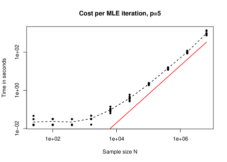
Figure 1: For $p=5$, cost per iteraton of MLE. The dashed curve is the average of $10$ replicates. The solid reference line is parallel to $N^{3/2}$.

Figure 2 shows total cost versus $N$ in a setting with $p=5$ averaged over $100$ data sets. The cost curve for the MLE computation looks different from Figure 1. It does not start out flat for small $N$. We found that the number of iterations required to find the MLE generally rose over the range $64\leqslant N\leqslant 6400$ and then declined gently thereafter.

From the analysis and empirical results, we find that a cost per iteration of $O(N^{3/2})$ is a realistic lower bound for the MLE code. The method of moments cost is $O(N)$ theoretically and appears to be proportional to $N$ empirically.

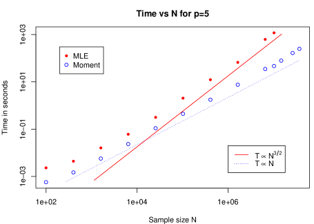
Figure 2: Computational cost for MLE and moments versus sample size $N$. There are reference lines parallel to $N^{3/2}$ and $N^{1}$.

Our computations were done with data generated in memory. In commercial applications, there could be a much larger time cost proportional to $N$ involved in reading the data from external storage. However, the $N^{3/2}$ cost component would be considerably larger at commercial scale, where $N$ is much larger than in our examples. For the method of moments it is straightforward to read and use the data in parallel even for large $N$.

A second computational issue arises with the linear mixed effects MLE. The code crashes on large enough data sets because the algorithm requires $O((R+C)^{2})$ memory. For $p=5$ we were unable to take the next step past $N=5120^{2}/4\doteq 6.5\times 10^{6}$. The program runs out of memory on our cluster. For $p=1$, it crashes for $N$ near $18$ million observations. The method of moments in Algorithm 1 has linear cost both theoretically and empirically and can be implemented in $O(R+C)$ memory. The difference is minor for our CPU time simulations that also keep all $N$ observations in memory, but it will be critical in large commercial applications.

6.2 Statistical efficiency

For statistical efficiency we considered $p=1$, $5$, $10$ and $20$. Sample sizes $N=100\times 4^{j}$ for $j=0,1,\dots,8$ were replicated $100$ times each. A few larger values of $N$ were replicated $10$ times each, though the MLE code would not run on all of the largest sample sizes we tried. The pattern in the results was the same for all of those $p$. We display results for $p=5$ in Figure 3. The MSEs for $\beta$ decay proportionally to $1/N$. The reference curves for variance components in Figure 3 are what we would expect from IID sampling of $a_{i}$, $b_{j}$ and $e_{ij}$, respectively namely $2\sigma_{A}^{4}/R$, $2\sigma_{B}^{4}/C$ and $2\sigma_{E}^{4}/N$ where $R=C=2\sqrt{N}$.

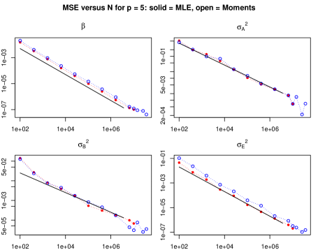
Figure 3: Mean squared errors for $\beta$, $\sigma^{2}_{A}$, $\sigma^{2}_{B}$ and $\sigma^{2}_{E}$ versus $N$. Reference lines for $\beta$ and $\sigma^{2}_{E}$ are parallel to $N^{-1}$. Reference lines for $\sigma^{2}_{A}$ and $\sigma^{2}_{B}$ are parallel to $N^{-1/2}$.

The parameter of greatest interest will ordinarily be $\beta$. The MLE has greater accuracy for $\beta$, as it must by the Gauss-Markov theorem. In this instance the MLE has about half the MSE that the method of moments does. For the variance components, the method of moments attains essentially the same MSE as the MLE does for $\sigma^{2}_{A}$ and $\sigma^{2}_{B}$. The MLE has greater efficiency for $\sigma^{2}_{E}$. In ordinary use we would want to know ratios of variance components and the uncertainty in such ratios is dominated by that in $\sigma^{2}_{A}$ and $\sigma^{2}_{B}$, where the two methods have comparable accuracy.

In this example, we saw a modest loss in statistical efficiency of $\hat{\beta}$ and $\hat{\sigma}^{2}_{E}$ and comparable accuracy for $\hat{\sigma}^{2}_{A}$ and $\hat{\sigma}^{2}_{B}$. These comparisons were run on data simulated from the Gaussian model that the MLE assumes. The method of moments does not require that assumption. Likelihood based variance estimates for variance components, such as $\widehat{\mathrm{Var}}(\hat{\sigma}^{2}_{A})$, can fail to be even asymptotically correct when the Gaussian model does not hold.

7 Conclusion and Future Work

We have proposed an algorithm for the two-factor linear mixed effects model with crossed covariance structure that provides consistent and asymptotically normal parameter estimates. It alternates twice between estimating the regression coefficients and estimating the variance components via the method of moments.

Unlike the available methods based on Bayes theorem or maximum likelihood, the moment estimates cost $O(N)$ time and $O(R+C)$ space. The variance estimate for $\hat{\beta}$ is obtained by substituting consistent estimates of $\sigma^{2}_{A}$, $\sigma^{2}_{B}$, and $\sigma^{2}_{E}$ into exact finite sample formulas for that variance matrix. The variance estimates for $\hat{\sigma}^{2}_{A}$, $\hat{\sigma}^{2}_{B}$, and $\hat{\sigma}^{2}_{E}$ are obtained by such a substitution in mildly conservative formulas from Gao and Owen, (2017). Here the usual root $n$ consistency from IID settings is replaced by a $1/\sqrt{\epsilon}$ consistency for $\epsilon=\max(\epsilon_{R},\epsilon_{C})$. Interpreting $1/\sqrt{\epsilon}$ as an effective sample size might be somewhat conservative because in theorems such as Theorem 2.1 the value of $\epsilon$ appears in upper bounds.

We exchange higher MSEs for an algorithm with cost only linear in the number of observations. We do not know how bad the efficiency loss might be in general, but we expect that when the pure error term $\sigma^{2}_{E}$ is meaningfully large that the loss will not be extreme. Also, if one of $\sigma^{2}_{A}$ and $\sigma^{2}_{B}$ very much dominates the other one, we can get a GLS estimate that accounts for the dominant source of correlation.

We anticipate that a martingale central limit theorem will apply to the variance component estimates $\hat{\sigma}^{2}_{A}$, $\hat{\sigma}^{2}_{B}$, and $\hat{\sigma}^{2}_{E}$. Some details will be in the forthcoming dissertation of the first author. We do not anticipate those variance components to be uncorrelated with $\hat{\beta}$ because the random variables $a_{i}$, $b_{j}$, and $e_{ij}$ do not need to have symmetric distributions.

This paper is a second step in developing big data versions of mixed model procedures such as the Henderson estimators. One followup step is to incorporate interactions between fixed and random steps, as the Henderson III model allows. Another is to incorporate interactions among latent variables. At present both kinds of interactions would serve to inflate $\sigma^{2}_{E}$. A third step is to adapt to binary responses, for instance by replacing the identity link in Model (1), with a logit or probit link. This third step is of value because many responses in e-commerce are categorical. One binary response of interest to Stitch Fix is whether the client keeps the item of clothing.

References

- Bates, (2014) Bates, D. (2014). Computational methods for mixed models. Technical report, Department of Statistics, University of Wisconsin–Madison. https://cran.r-project.org/web/packages/lme4/vignettes/Theory.pdf.
- Bates, (2016) Bates, D. (2016). Linear mixed-effects models in Julia. https://github.com/dmbates/MixedModels.jl.
- Bezanson et al., (2017) Bezanson, J., Edelman, A., Karpinski, S., and Shah, V. B. (2017). Julia: A fresh approach to numerical computing. SIAM Review, 59(1):65–98.
- Fox, (2013) Fox, C. (2013). Polynomial accelerated MCMC and other sampling algorithms inspired by computational optimization. In Dick, J., Kuo, F. Y., Peters, G. W., and Sloan, I. H., editors, Monte Carlo and Quasi-Monte Carlo Methods 2012, pages 349–366. Springer, Berlin.
- Gao and Owen, (2017) Gao, K. and Owen, A. B. (2017). Efficient moment calculations for variance components in large unbalanced crossed random effects models. Electronic Journal of Statistics. (To appear).
- Hager, (1989) Hager, W. W. (1989). Updating the inverse of a matrix. SIAM Review, 31(2):221–239.
- Henderson, (1953) Henderson, C. R. (1953). Estimation of variance and covariance components. Biometrics, 9(2):226–252.
- Imbens and Rubin, (2015) Imbens, G. W. and Rubin, D. B. (2015). Causal inference in statistics, social, and biomedical sciences. Cambridge University Press, Cambridge.
- Ioannidis, (2005) Ioannidis, J. P. A. (2005). Why most published research findings are false. PLoS medicine, 2(8):e124.
- Marshall and Olkin, (1990) Marshall, A. W. and Olkin, I. (1990). Matrix versions of the Cauchy and Kantorovich inequalities. Aequationes Mathematicae, 40(1):89–93.
- Powell, (2009) Powell, M. J. D. (2009). The BOBYQA algorithm for bound constrained optimization without derivatives. Technical Report NA2009/06, University of Cambridge.
- Provost and Fawcett, (2013) Provost, F. and Fawcett, T. (2013). Data science and its relationship to big data and data-driven decision making. Big Data, 1(1):51–59.
- Raudenbush, (1993) Raudenbush, S. W. (1993). A crossed random effects model for unbalanced data with applications in cross-sectional and longitudinal research. Journal of Educational and Behavioral Statistics, 18(4):321–349.
- Roberts and Sahu, (1997) Roberts, G. O. and Sahu, S. K. (1997). Updating schemes, correlation structure, blocking and parameterization for the Gibbs sampler. Journal of the Royal Statistical Society, Series B, pages 291–317.
- Scott et al., (2016) Scott, S. L., Blocker, A. W., Bonassi, F. V., Chipman, H. A., George, E. I., and McCulloch, R. E. (2016). Bayes and big data: The consensus Monte Carlo algorithm. International Journal of Management Science and Engineering Management, 11(2):78–88.
- Searle et al., (1992) Searle, S. R., Casella, G., and McCulloch, C. E. (1992). Variance components. John Wiley & Sons, New York.
- Varian, (2014) Varian, H. R. (2014). Big data: New tricks for econometrics. The Journal of Economic Perspectives, 28(2):3–27.
- Wasserstein and Lazar, (2016) Wasserstein, R. L. and Lazar, N. A. (2016). The ASA’s statement on -values: context, process, and purpose. Americal Statistician, 70(2):129–133.