On a relation between roughening and coarsening

Abstract

We argue that a strict relation exists between two in principle unrelated quantities: The size of the growing domains in a coarsening system, and the kinetic roughening of an interface. This relation is confirmed by extensive simulations of the Ising model with different forms of quenched disorder, such as random bonds, random fields and stochastic dilution.

Slow relaxation is a feature found in a variety of physical systems including randomly stirred fluids, ballistic aggregation, magnetic flux lines in superconductors sug_pl1 , directed polymers and manifolds in random media Kard97 ; Kard87 ; Fish91 , phase-ordering puri09 ; Puri04 ; Bray91 ; corbcrp ; zanreview ; Paul04 ; Henk08 ; Sic08 ; Corb02 ; Lip10 ; Corb11 ; Corb12 ; Corb13 ; sug_pl2 and others. In these cases the evolution is characterized by scale-free power-law behaviors and the equilibrium state is approached on a timescale that diverges in the thermodynamic limit. In this Letter we focus on two paradigms of slow relaxation, i) the evolution a disordered ferromagnet after a temperature quench and ii) the roughening of an interface in a medium. The aim of the paper is to show a strict correspondence between i) and ii).

A unified description of the two problems above can be arrived at by considering a ferromagnetic system, namely a collection of interacting Ising spins $S_{i}$ on the sites $i$ of a lattice. For such a system the usual para-ferromagnetic transition occurs at some critical temperature $T_{c}$. Quenched disorder, in the form of random fields or bonds, stochastic dilution or other sources of randomness, can be present provided that the low-temperature ordered phase is preserved. The two kinds of slow evolution i) and ii) mentioned above can be observed in such a model at low temperature $T<T_{c}$ by preparing the sample with the initial condition (at time $t=0$) in the following two ways:

i) The value of each spin $S_{i}=\pm 1$ is randomly chosen and is uncorrelated from the others, corresponding to the equilibrium state of the ferromagnet at infinite temperature. This protocol amounts to the instantaneous quench of the system from the initial temperature $T_{i}=\infty$ to the final temperature $T<T_{c}$. As it is well known, a coarsening stage is observed puri09 ; Puri04 ; Bray94 ; Bray91 ; corbcrp ; zanreview ; Paul04 ; Henk08 ; Sic08 ; Corb02 ; Lip10 ; Corb11 ; Corb12 ; Corb13 ; sug_pl2 with growing magnetic domains of size ${\cal L}(t,\epsilon,\ell)$, where $\ell$ is the system size and we indicate generically by $\epsilon$ the strength of the disorder. For example, denoting by $L$ the domains size in an infinite system ($L(t,\epsilon)\equiv{\cal L}(t,\epsilon,\ell=\infty)$), in a pure (non disordered) magnet ($\epsilon=0$) one usually has $L(t,0)\propto t^{1/z}$ (with $z=2$ with a non-conserved order parameter). Dynamical scaling Bray94 implies that $L$ is the only dominant length at large times.

ii) The system is divided into two halves, as for instance by the diagonal in a square system, and spins are set to the value $S_{i}=+1$ in one half and $S_{i}=-1$ in the other. Appropriate boundary conditions are provided in such a way that the spanning interface seeded by the initial condition remains at all times (e.g. if the system is divided by the diagonal anti-periodic boundary conditions are used). The main feature of the process ii) is the kinetic roughening of the interface which, in a pure system, is described by the usual Family-Vicksek scaling relation FV ; Kolt

$$W(t,\ell)=A(T)\,\xi(t)^{\alpha}{\cal V}\left(\frac{\ell}{\xi(t)}\right),$$ (1)

where $W(t,\ell)$ is the interface width, or roughness, namely the root mean square displacement with respect to the initial straight configuration (see further on for an operative definition), $\xi(t)=t^{1/Z}$ is a quantity with dimensions of a length, $A$ is a temperature-dependent constant (the width of an interface in equilibrium in a box of unitary length $\ell=1$), $\alpha$ and $Z$ are the roughening and the dynamical exponent. For the Edwards-Wilkinson universality class, corresponding to an interface in a magnetic system without conservation of the order parameter, one has $Z=2$. ${\cal V}(x)$ is a scaling function with the limiting behaviors

$$\left\{\begin{array}[]{l}{\cal V}(x)=const.\hskip 18.49411pt,\hskip 14.22636pt\mbox{for}\,\,\,x\gg 1\\ {\cal V}(x)=x^{\alpha}\hskip 34.14322pt,\hskip 14.22636pt\mbox{for}\,\,\,x\ll 1\end{array}\right.$$ (2)

Let us remark that $W(t,\ell)$, considered in the evolution i) must not be confused with the width of interfaces separating different domains during the coarsening evolution i). However, both the evolutions i) and ii) are determined by the flip of spin on interfaces which are governed by the same microscopic rules. This will be important in the following. Notice also that in the pure case, by running the two processes i) and ii) from $t=0$ in parallel and measuring $L$ in i) and $\xi$ in ii) one would find

$$L(t,\epsilon=0)\propto\xi(t)$$ (3)

because $L\sim t^{1/z}$ and $\xi\sim t^{1/Z}$ with $z=Z$ in this case. This result highlights the robustness of the fundamental length responsible of dynamical scaling under strong variations of the initial condition, as when passing from system i) to ii). In this paper we shall carry out a detailed study of this remarkable result by extending the investigation to the vast area of systems with quenched randomness.

An important point that we want to address is how Eqs. (1,2) change in the presence of quenched randomness. Quite generically Lip10 ; Corb11 ; Corb12 ; Corb13 ; Corb02 ; corbcrp this additional source of disorder introduces an extra length $\lambda(\epsilon)$ in the problem. The actual meaning of this quantity depends on the system at hand: In the presence of quenched impurities, for instance, $\lambda$ can be associated to the typical distance among two of them. One has usually the property

$$\lim_{\epsilon\to 0}\lambda(\epsilon)=\infty,$$ (4)

as it can be easily understood in the case of quenched impurities. Clearly, a possible generalization of Eq. (2) must keep into account the presence of this additional length $\lambda$. Furthermore, it is well known schehr that disorder modifies the growth of correlations $\xi$ (as will be clear from our data, see discussion later) with respect to the behavior in a pure system.

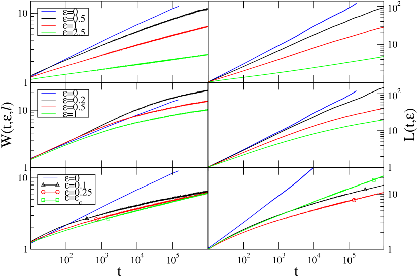
Figure 1: (Color online) $W(t,\epsilon,\ell=\infty)$ (left three panels) and $L(t,\epsilon)$ (right three panels) are plotted against time on a double-logarithmic plot for the RBIM (top two panels), the RFIM (central two panels) and the SDIM (bottom two panels). For the RBIM the values of disorder displayed are $\epsilon=0$ (pure case, blue), $\epsilon=0.5$ (black), $\epsilon=1$ (red), $\epsilon=2.5$ (green), from top to bottom. For the RFIM the disorder values are $\epsilon=0$ (pure case, blue), $\epsilon=0.2$ (black), $\epsilon=0.5$ (red), $\epsilon=1$ (green), from top to bottom. For the SDIM the dilution values are $\epsilon=0$ (pure case, blue) $\epsilon=0.1$ (black with a triangle), $\epsilon=0.25$ (red with a circle) and $\epsilon=\epsilon_{c}$ (green with a square).

Borrowing from the fact that in the pure case one can replace $\xi$ with the domains size $L$ of the corresponding process i), according to Eq. (3), we infer that the proper generalization of the scaling (1) to systems with quenched disorder is a two-parameter scaling with typical lengths $L(t,\epsilon)$ and $\lambda(\epsilon)$, namely

$$W(t,\epsilon,\ell)=A(T,\epsilon)\,L(t,\epsilon)^{\alpha}{\cal W}\left(\frac{\ell}{L(t,\epsilon)},\frac{\lambda(\epsilon)}{L(t,\epsilon)}\right),$$ (5)

with a scaling function such that

$$\lim_{y\to\infty}{\cal W}(x,y)={\cal V}(x),$$ (6)

where ${\cal V}(x)$ is given in Eq. (2) in order to recover Eq. (1) when disorder is absent (using Eq. (4)).

Eq. (5) is a bridge between two a priori unrelated quantities, the width of an isolated roughening interface (on the l.h.s.) and the size of the domains in a coarsening process (on the r.h.s). It is the central statement of this paper: Its verification in different systems will be the main issue below. Before doing that, let us stress that the form (5) is different from a usual two-parameter scaling, because the strength of disorder enters not only through the extra length $\lambda(\epsilon)$ but also in the quantity $L(t,\epsilon)$. We will show that Eq. (5) describes the whole pattern of behaviors of magnetic systems with different form of quenched disorder and for any strength $\epsilon$ of their randomness.

To start with, Eq. (5) is obviously correct in the pure case $\epsilon=0$, since due to Eqs. (4,6) one recovers Eq. (1) when disorder is absent. This shows that, both in Eqs. (1) and (5), $\alpha$ is the roughening exponent of the pure case which is obviously independent of disorder. In the opposite limit $\epsilon\to\infty$, when disorder is very strong, the roughening exponent is expected to take a different value $\zeta\neq\alpha$ Kard97 . This is accounted for by the scaling (5) if $\lim_{y\to 0}y^{\zeta-\alpha}{\cal W}(x,y)\sim\omega(x)$, where $\omega$ is another function with asymptotic behaviors analogous to those (2) of ${\cal V}$. Summarizing, one has

$$W(t,\epsilon,\ell)=A(T,\epsilon)\cdot\left\{\begin{array}[]{l}L(t,\epsilon)^{\alpha}\,{\cal V}(x)\,,\hskip 34.14322pt\mbox{for}\,\,y\gg 1\,[w]\\ L(t,\epsilon)^{\zeta}\,\lambda(\epsilon)^{\alpha-\zeta}\,\omega(x)\,,\mbox{for}\,\,y\ll 1\,\,[s],\end{array}\right.$$ (7)

where the two regimes $y\gg 1$ and $y\ll 1$ are denoted as $w$ and $s$ for the reasons that will be explained below.

In the following we will check the validity of Eq. (5) in the two-dimensional Ising model with random fields, random bonds and site dilution. All these models can be described by the Hamiltonian $H=-\sum_{\langle ij\rangle}J_{ij}n_{i}n_{j}S_{i}S_{j}-\sum_{i}h_{i}S_{i}$ where $i$ ($j$) are sites on a square lattice and $\langle ij\rangle$ are nearest neighbors couples. From this Hamiltonian the random bond Ising model (RBIM) corbcrp ; Corb11 is obtained by taking $n_{i}=1$ $\forall i$, $h_{i}=0$ $\forall i$ and $J_{ij}$ random variables uniformly distributed in $[J-\epsilon\,T,J+\epsilon\,T]$, with $\epsilon\,T<J$. The random field Ising model (RFIM), on the other hand, amounts to $n_{i}=1$ $\forall i$, $J_{ij}=J$ $\forall\langle ij\rangle$ and $h_{i}=\pm\epsilon\,T$ uncorrelated random variables with equal probability. Finally, the site diluted Ising model (SDIM) is obtained by taking a uniform $J_{ij}=J$, $h_{i}\equiv 0$ and $n_{i}$ uncorrelated random variables such that $n_{i}=0$ with probability $\epsilon$ (the dilution) and $n_{i}=1$ with probability $1-\epsilon$.

The systems above are evolved numerically, both for process i) and ii) by means of single spin flips with Glauber transition rates up to $10^{6}$ Montecarlo steps. Besides, we prevent the flipping of bulk spins which are aligned with all the nearest neighbors. In case ii) this guarantees that the interface is unique at all times. In case i) this modified dynamics has been used in several studies nobulk of phase-ordering where it was shown that it does not alter the behavior of the quantities we are interested in, in the limit of small temperatures that will be considered below. It has also the advantage to speed-up the computation.

Let us start by discussing the details of the simulations for the phase-ordering kinetics, namely process i). For this problem we have performed a set of numerical runs where phase ordering dynamics occurs in a system of size $\ell=2000\,a_{0}$, where $a_{0}$ is the lattice-spacing and we set $a_{0}=1$ hereafter. Since we have checked that this sample is sufficiently large to avoid finite-size effects in the time range considered, one has ${\cal L}(t,\epsilon,\ell=2000)\simeq{\cal L}(t,\epsilon,\ell=\infty)=L(t,\epsilon)$. The characteristic size $L$ – one building block of Eq. (5) – is obtained as the inverse excess energy $L(t,\epsilon)\sim[E(t)-E(\infty)]^{-1}$, where $E(\infty)$ is the energy of the target equilibrium state Lip10 ; Corb11 ; Corb13 and $E(t)$ is the energy at time $t$. This is a standard way to evaluate $L(t,\epsilon)$ in coarsening systems: it is based on the fact that the interior of domains is in equilibrium and the excess energy is stored on the interface, so $E(t)-E(\infty)$ is proportional to their total length. This in turn is given by the length of a single domain’s boundary ($\propto L$) times the number of such domains ($\propto L^{-2}$), from which the above relation between $L(t,\epsilon)$ and the excess energy is obtained.

Phase-ordering in random ferromagnets has been the subject of a number of recent studies Paul04 ; Henk08 ; Sic08 ; Corb02 ; Lip10 ; Corb11 ; Corb12 ; Corb13 ; corbcrp ; sug_pl2 to which we refer for a detailed discussion. For the scope of the present study what has to be recalled is the existence of a crossover length $\lambda(\epsilon)$ such that $L(t,\epsilon)$ crosses over from an early regime where the growth-law is still algebraic (although with an exponent that may depend on $\epsilon$ and $T$) for $L(t,\epsilon)\ll\lambda(\epsilon)$, to a late logarithmic growth $L(t,\epsilon)\gg\lambda(\epsilon)$. We will refer to these two regimes in a compact way as $w$ (standing for weak, as referred to the effects of disorder, since the growth-law remains algebraic) and $s$ (standing for strong), respectively. Let us also mention that $T_{c}=0$ for the RFIM in $d=2$, meaning that coarsening in this system is interrupted after a time which diverges in the $T\to 0$ limit. In all the cases considered here this time is far beyond the times accessed in the simulations.

Regarding process ii), indicating with $(m,n)$ the (horizontal and vertical) coordinate of a lattice site $i$, the width is evaluated as $W(t,\epsilon,\ell)=(\ell/a_{0})^{-1}\sum_{n=1}^{\ell}\sqrt{w_{n}(t)^{2}}$. Here $w_{n}(t)$ is the distance travelled by the portion of interface, with vertical coordinate $n$, in the time interval $[0,t]$.

In order to check the scaling relation (5), for the single interface, we have considered different system sizes $\ell\in[4,1000]$. We observe that, in the $T\to 0$ limit we consider, the interface roughens almost independently of $T$. This is at variance with what observed in continuum theories of kinetic roughening upton , meaning that the discrete character of our model is relevant at such low temperatures.

Due to the presence of the two arguments in the scaling function of Eq. (5) its verification would in principle require, for any of the disordered models introduced above, a complete scan of the three-dimensional parameter-space $t,\epsilon,\ell$ and the determination of the scaling arguments $x=\ell/L$, $y=\lambda/L$. Since this is out of reach, we mainly focus on the limits $y\gg 1$ and $y\ll 1$, corresponding to the regimes $w$ and $s$ defined above, so that Eq. (5) simplifies to the couple of forms in (7) where the scaling functions ${\cal V}$ and $\omega$ depend on a single scaling variable.

RBIM) We start this program from the RBIM. In this case it was shown in Corb11 that the crossover from the regime $w$ to the one $s$ is delayed to such huge times that in simulations the condition $\lambda(\epsilon)/L(t,\epsilon)\gg 1$ is always met, namely the system is described at any reasonably accessible time by the regime $w$ of Eq. (7). This is very neatly observed in the upper-right panel of Fig. 1, where power growth-laws of $L(t)$ are observed in the range of simulated times and there is no indication of a crossover to a slower (i.e. logarithmic) growth, typical of regime $s$, for any choice of $\epsilon$. Therefore, by plotting $L(t,\epsilon)^{-\alpha}\,W(t,\epsilon,\ell)$, with the $d=2$ Edwards-Wilkinson roughening exponent $\alpha=1/2$, against $x=\ell/L(t,\epsilon)$ for any choice of $\epsilon$ one should find data collapse among curves obtained with different values of $\ell$. Furthermore, upon changing $\epsilon$ one expects only to observe a different prefactor $A(\epsilon,T)$ which, plotting on a double log scale, amounts to a vertical shift.

As shown in the first panel of Fig. 2 all these features are very well verified by the numerical data (notice that we use here $1/x$ on the horizontal axis, not $x$). Moreover, the exponent $\alpha=1/2$ can also be read out from the large $x$ behavior (left part of the figure) of the scaling function, which grows as $x^{\alpha}$ according to Eq. (5) and to the second of Eqs. (2) (this is drawn as a blue-dotted line in the figure). We stress the highly non-trivial nature of the scaling we have verified, since it allows us to collapse (apart from the shift due to $A$) curves relative to different disorder strengths for which the growth-exponent of the $L$’s (and hence of $W$) varies by a factor as large as three, as can be detected in the upper-right panel of Fig. 1.

Regarding the constant $A$ it turns out to be very weakly dependent on $\epsilon$. Indeed the curves for different values of $\epsilon$ are basically superimposing (however, for a better presentation, in Fig. 2 curves with different $\epsilon$ have been displaced vertically, see caption). A similar behavior of $A$ is found also for the other two models (RFIM and SDIM) discussed below.

Let us now comment on what we anticipated below Eq. (4), namely the fact that in system ii) the growth of correlations in the presence of disorder is modified with respect to the behavior $\xi(t)$ holding in the pure case. Indeed, if the growth was the same as in the pure case, and since $\alpha=1/2$, one should observe an increase $W(t,\epsilon,\ell=\infty)\sim\xi(t)^{\alpha}\sim t^{1/4}$ of the roughness in an infinite system in the regime $w$ we are considering, according to Eqs. (4,6). This is clearly observed in the upper-left panel of Fig. 1 only in the pure case $\epsilon=0$, as expected, while a completely different behavior is displayed for any disorder strength $\epsilon\neq 0$. One arrives at the same conclusion by considering the different disordered models that are discussed below.

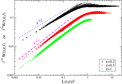
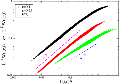
Figure 2: (Color online) Upper panel- The parametric plot $\ell^{-\alpha}W(t,\epsilon,\ell)$ vs $L(t,\epsilon)/\ell$ is plotted for the RBIM with three disorder values $\epsilon=0.5$ (black), $\epsilon=1$ (red), $\epsilon=2.5$ (green) from top to bottom. For each $\epsilon$ we consider different values of $\ell$ given by $\ell=5+1.2^{j}$, where $j$ is an integer in the range $[0:23]$, represented by different symbols. The blue-dotted line is the power law behavior $x^{1/2}$. Here and in the other panels curves relative to different values of $\epsilon$ are displaced vertically (data are multiplied by an arbitrary constant) for a better presentation. Central Panel - As in the upper panel for the RFIM with disorder values $\epsilon=0.2$ (black), $\epsilon=0.5$ (red), $\epsilon=1$ (green) from top to bottom. For this model, data collapse is obtained by plotting $\ell^{-\alpha}W(t,\epsilon)$ for $\epsilon=0.2$ and $\ell^{-\zeta}W(t,\epsilon)$ for $\epsilon=0.5$ and $\epsilon=1$. The blue-dotted line and the magenta dashed lines are the power law behavior $x^{1/2}$ and $x^{2/3}$, respectively. Lower Panel - As in the other panels but for the SDIM for three different dilution values $\epsilon=0.1$ (black), $\epsilon=0.25$ (red) and $\epsilon=\epsilon_{c}$ (green). For this model, data collapse is obtained by plotting $\ell^{-\alpha}W(t,\epsilon)$ for $\epsilon=\epsilon_{c}$ and $\ell^{-\zeta}W(t,\epsilon)$ for $\epsilon=0.1$ and $\epsilon=0.25$. The blue-dotted line and the magenta dashed lines are the power law behaviors $x^{1/2}$ and $x^{2/3}$, respectively.

RFIM) Due to its delayed crossover the RBIM was previously used as a benchmark to verify Eq. (7) in the regime $w$. In order to access the regime $s$, we will now focus on the RFIM where, since Corb12 $\lambda(\epsilon)\simeq\epsilon^{-2}$, one can arrange the parameter $\epsilon$ (the amplitude of the random field (in units of $T$), as specified below Eq. (7)) in order for the crossover from $w$ to $s$ to occur in the range of simulated times. Before doing that, in order to match with what we observed for the RBIM, we set $\epsilon$ to a value as small as $\epsilon=0.2$ for which the crossover time is larger than the simulated times. This is confirmed by inspection of the central-right panel of Fig. 1). Here one sees that also for such a small value of $\epsilon$ the behavior of the system is radically different from the non-disordered case, since $L$ grows with an effective exponent $1/z\simeq 0.4$, definitively smaller than for $\epsilon=0$. However, there is no manifestation of a crossover to the slower (i.e. logarithmic) growth-law characteristic of the $s$ regime (which, instead, is clearly observed in the same panel for the two larger values of $\epsilon$, as will be discussed later). In this small-$\epsilon$ case, since we are yet confined into the $w$ regime, we expect to observe a situation analogous to one discussed previously regarding the RBIM. This is in fact what one observes in the second panel of figure 2 (upper set of data, in black): curves for different values of $\ell$ can be collapsed by using the rescaling $w$ of Eq. (7), with $\alpha=1/2$. We interpret the somewhat poorer quality of the collapse, as compared to the RBIM, as due to the fact that even for such a small value of $\epsilon$ we have not been able to push the crossover time well beyond the end of the simulation.

The situation is radically different when values of $\epsilon$ as large as $\epsilon=0.5$ and $\epsilon=0.8$ are used. In this case the central-left panel of Fig. 1 shows that a crossover from $w$ to $s$ is observed quite early. Actually, it occurs so early that collapsing the curves by means of the scaling $w$ of Eq. (7) turns out to be impossible. Instead a good mastercurve is obtained by using the form $s$ of Eq.(7), with $\zeta=2/3$. We recall that this is the asymptotic roughening exponent expected for a class of models where disorder acts only on the interfaces noirough ; surfbulk . The same exponent is also observed pre-asymptotically in the present model noirough , despite an asymptotic value $\zeta=1$ is expected for very large times noirough ; surfbulk . The good scaling obtained with $\zeta=2/3$ signals that the truly asymptotic behavior with $\zeta=1$ is located much further in time. Again, we stress the notable character of the collapse as compared to the very different forms of $L$ and of $W$ shown in the central panels of Fig. 1, as $\epsilon$ is changed.

SDIM) It is known that in this model disorder introduces two characteristic lengths Corb13 . In a nutshell, $\lambda_{1}(\epsilon)\propto\epsilon^{-1/d}$ represents the average distance between vacancies, while $\lambda_{2}(\epsilon)\propto(\epsilon_{c}-\epsilon)^{-\nu}$, where $\epsilon_{c}=1-p_{c}\simeq 0.4072$ is the vacancy density at percolation and $\nu=4/3$ the critical exponent, represents the coherence length over which the fractal percolative structure extends. In the presence of two lengths associated to the disorder Eq. (5) can be generalized to

$$W(t,\epsilon,\ell)=A(T,\epsilon)\,L(t,\epsilon)^{\alpha}{\cal W}\left(\frac{\ell}{L(t,\epsilon)},\frac{\lambda_{1}(\epsilon)}{L(t,\epsilon)},\frac{\lambda_{2}(\epsilon)}{L(t,\epsilon)}\right).$$ (8)

The SDIM offers an interesting example where disorder introduces a couple of lengths allowing one to verify Eq. (8) in this more complex framework.

As it is clear from their behavior, in the opposite limits $\epsilon\to 0$ or $\epsilon\to\epsilon_{c}$ either one or the other length diverges, meaning that – when this occurs – the regime $w$ of Eq. (7) extends to very long times. On the other hand, for values of $\epsilon$ well inside the range $[0,\epsilon_{c}]$, such as, for instance, $\epsilon=0.25$, any length associated to the disorder becomes small and the regime $s$ is entered very soon. A first consequence of this structure is that for $\epsilon=0.25$ the growth-law of $L(t,\epsilon)$ turns out to be slower, since it is soon logarithmic, than in the cases closer either to $\epsilon=0$ or $\epsilon=\epsilon_{c}$. This is very clearly seen in the lower-right panel of Fig. 1. A second consequence is that we expect to observe the form $w$ of Eq. (7) for $\epsilon=0$ or $\epsilon_{c}-\epsilon\ll 1$ (say, $\epsilon=\epsilon_{c}$), while for intermediate values of $\epsilon$ collapse should be obtained with the scaling $s$ of Eq. (7). This is very well observed in the third panel of Fig. 2, confirming again Eq. (8). Let us emphasize that this result, obtained in a case with a complex structure with more than one length associated to quenched disorder, is a highly non-trivial and stringent check providing a further strong indication of the general validity of Eq. (8).

Eq. (5) establishes a direct correspondence between roughness of interfaces and size of growing domains holding in a variety of systems, pure or with different kind of quenched randomness. One might wonder which is the physical reason behind this. A possible explanation is the following: focusing for simplicity on the pure case, it is well known that the quantity $\xi(t,\epsilon=0)$ appearing in Eq. (1) describes a longitudinal (i.e. along the surface) coherence length growing indefinitely in a system of infinite size ($\ell=\infty$). Since the two processes i) and ii) are governed by a unique underlying model, an analogous coherence length could be expected to develop also on the boundaries of the coarsening domains of case i) (still with $\ell=\infty$), as shown pictorially in the lower part of Fig. 3. Dynamical scaling Bray94 implies that there must be a unique relevant length, suggesting $\xi\simeq L$. This shows that $\xi$ and $L$ are basically the same object and that their common behavior $\xi\sim L\sim t^{1/z}$ in the pure case is not a coincidence, allowing one to interchange them when writing the Family-Vicksek scaling (1). A similar argument to infer the roughness of domain’s boundaries in a coarsening system is quoted in upton . This basically assumes that each interface in system i) can be mapped on one of those of process ii) in equilibrium in a system whose size $l$ is kept adiabatically equal to the domain’s size $L(t)$ of process i). Since in equilibrium it is $W^{eq}(l)\sim l^{\alpha}$, this implies that in a coarsening system the domain walls have a roughness $W(t)\sim W^{eq}(l=L(t))\sim L^{\alpha}(t)\sim t^{\alpha/z}$. Our statement is partly different. Indeed the argument we propose only relies on the presence of dynamical scaling, and there is no need to make any equilibration hypotheses. Furthermore our conclusions are more general, since on one hand Eq. (5) applies not only to the interfaces of a coarsening system, but also to different situations as the one encountered in the process ii) and others. Furthermore Eq. (5) is a complete scaling form describing the process from the out-of-equilibrium stage up to the stationary asymptotic state of the interface as well as the intermediate crossover, incorporating in addition also the finite size effects due to $\ell<\infty$. Clearly, the argument above – repeated in the presence of quenched randomness with the further ingredient of the extra length $\lambda$ – generalizes the conclusions above to disordered systems.

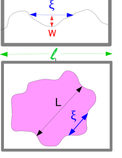
Figure 3: (Color online) Sketch of a single interface spanning a system (upper part) and of a domain during coarsening (lower part).

In this paper we have shown a strict relation between two in principle unrelated quantities, the size of the growing domains in a coarsening system, and the roughening of an interface. This relation, which has been confirmed numerically in a variety of disordered systems, opens the way to a cross-fertilization between the fields of phase-ordering and kinetic roughening, allowing one to borrow knowledge from one side to the other, possibly improving the state of the art of our comprehension of these processes. Because of that, a deeper understanding of this relation and of its domain of applicability would be desirable and represents an interesting subject for future research.

References

- (1) M. Pleimling and U.C. Tauber, Phys. Rev. B 84, 174509 (2011); H. Assi et. al., Phys. Rev. E 92, 052124 (2015).
- (2) M. Kardar, in Dynamics of Fluctuating Interfaces and Related Phenomena, edited by D. Kim, H. Park, and B. Kahng, World Scientific, Singapore, 1997.
- (3) M. Kardar and Y.-C. Zhang, Phys. Rev. Lett. 58, 2087 1987. J. M. Kim, M. A. Moore, and A. J. Bray, Phys. Rev. A 44, 2345 (1991).
- (4) D. S. Fisher and D. A. Huse, Phys. Rev. B 43, 10728 (1991).
- (5) A.J. Bray, Adv. Phys.43, 357 (1994).
- (6) S. Puri, in Kinetics of Phase Transitions, edited by S. Puri and V. Wadhawan, CRC Press, Boca Raton (2009), p. 1.
- (7) S. Puri, Phase Transitions 77, 469 (2004). S. Puri, D. Chowdhury and N. Parekh, J. Phys. A 24, L1087 (1991); S. Puri and N. Parekh, J. Phys. A 25, 4127 (1992).
- (8) A.J. Bray and K. Humayun, J. Phys. A 24, L1185 (1991).
- (9) F. Corberi, Compt. Ren. Phys. 16, 332 (2015).
- (10) G. Schehr and P. Le Doussal, Phys. Rev. Lett. 93, 217201 (2004). G. Schehr and H. Rieger, Phys. Rev. B 71, 184202 (2005).
- (11) M. Zannetti, Chapter 5 in ”Kinetics of Phase Transitions” S.Puri and V.Wadhawan Eds., CRC Press Taylor Francis Group (2009). ISBN 13:978084939065
- (12) R. Paul, S. Puri and H. Rieger, Europhys. Lett. 68, 881 (2004); R. Paul, S. Puri and H. Rieger, Phys. Rev. E 71, 061109 (2005); R. Paul, G. Schehr and H. Rieger, Phys. Rev. E 75, 030104(R) (2007).
- (13) M. Henkel and M. Pleimling, Europhys. Lett. 76, 561 (2006); Phys. Rev. B 78, 224419 (2008).
- (14) A. Sicilia, J. J. Arenzon, A. J. Bray and L. F. Cugliandolo, Europhys. Lett. 82, 1001 (2008); M. P. O. Loureiro, J. J. Arenzon, L. F. Cugliandolo, and A. Sicilia, Phys. Rev. E 81, 021129 (2010).
- (15) F. Corberi, A. de Candia, E. Lippiello and M. Zannetti, Phys. Rev. E 65, 046114 (2002); F. Corberi, A. de Candia, E. Lippiello and M. Zannetti, Physica A 314, 454 (2002).
- (16) E. Lippiello, A. Mukherjee, S. Puri and M. Zannetti, Europhys. Lett. 90, 46006 (2010).
- (17) F. Corberi, E. Lippiello, A. Mukherjee, S. Puri and M. Zannetti, J. Stat. Mech.: Theory and Experiment P03016 (2011).
- (18) F. Corberi, E. Lippiello, A. Mukherjee, S. Puri, and M. Zannetti, Phys. Rev. E 85, 021141 (2012).
- (19) F. Corberi, E. Lippiello, A. Mukherjee, S. Puri, and M. Zannetti, Phys. Rev. E 88, 042129 (2013).
- (20) H. Park and M. Pleimling, Phys. Rev. B 82, 144406 (2010); H. Park and M. Pleimling, Eur. Phys. J. B 85, 300 (2012)
- (21) F. Family and T. Vicsek: J. Phys. A: Math. Gen. 18, 75 (1985).
- (22) A.B. Kolton, A. Rosso and T. Giamarchi, Phys. Rev. Lett. 95, 180604 (2005).
- (23) F. Corberi, E. Lippiello, and M. Zannetti, Phys. Rev. E 63, 061506 (2001); Eur. Phys. J. B 24, 359 (2001); Phys.Rev. E 68, 046131 (2003); Phys.Rev. E 78, 011109 (2008); E. Lippiello, F. Corberi, A. Sarracino, and M. Zannetti, Phys. Rev. E 78, 041120 (2008); F. Corberi, and L.F. Cugliandolo, J. Stat. Mech. P05010 (2009).
- (24) T. Nattermann Europhys. Lett. 4, 1241 (1987). M.E. Fisher, J. Chem. Soc., Faraday Trans. 82, 1569 (1986). M. Kardar, J. Appl. Phys. 61, 3601 (1987). T. Halpin-Healy, Phys. Rev. Lett. 62, 442 (1989); Phys. Rev. A 42, 711 (1990). D. A. Huse and C. L. Henley, Phys. Rev. Lett. 54, 2708 (1985); M. Kardar, ibid. 55, 2923 (1985); D. A. Huse, C. L. Henley, and D. S. Fisher, ibid. 55, 2924 (1985).
- (25) F. Corberi, E. Lippiello, and M. Zannetti, J. Phys. A: Math. Theor. 49, 185001 (2016).
- (26) D. B. Abraham and P. J. Upton, Phys. Rev. B 39, 736 (1989).