Date: 25 October 2016

MuSIC : delivering the world’s most intense muon beam

S. Cook¹, R. D’Arcy¹, A. Edmonds¹, M. Fukuda², K. Hatanaka², Y. Hino³,

Y. Kuno³, M. Lancaster¹, Y. Mori⁴, T. Ogitsu⁵, H. Sakamoto³, A. Sato³,

N.H. Tran³, N.M. Truong³, M. Wing¹, A. Yamamoto⁵ and M. Yoshida⁵

¹Department of Physics and Astronomy, UCL, Gower Street, London, WC1E 6BT, UK

²Research Center for Nuclear Physics (RCNP), Osaka University, Osaka, Japan

³Department of Physics, Graduate School of Science, Osaka University, Osaka, Japan

⁴Kyoto University Reactor Research Institute (KURRI), Kyoto, Japan

⁵High Energy Accelerator Research Organization (KEK), Tsukuba, Japan

A new muon beamline, muon science innovative channel (MuSIC), was set up at the Research Center for Nuclear Physics (RCNP), Osaka University, in Osaka, Japan, using the 392 MeV proton beam impinging on a target. The production of an intense muon beam relies on the efficient capture of pions, which subsequently decay to muons, using a novel superconducting solenoid magnet system. After the pion-capture solenoid the first $36^{\circ}$ of the curved muon transport line was commissioned and the muon flux was measured. In order to detect muons, a target of either copper or magnesium was placed to stop muons at the end of the muon beamline. Two stations of plastic scintillators located upstream and downstream from the muon target were used to reconstruct the decay spectrum of muons. In a complementary method to detect negatively-charged muons, the X-ray spectrum yielded by muonic atoms in the target were measured in a germanium detector. Measurements, at a proton beam current of 6 pA, yielded $(10.4\pm 2.7)\times 10^{5}$ muons per Watt of proton beam power ($\mu^{+}$ and $\mu^{-}$), far in excess of other facilities. At full beam power (400 W), this implies a rate of muons of $(4.2\pm 1.1)\times 10^{8}$ muons s^-1, amongst the highest in the world. The number of $\mu^{-}$ measured was about a factor of 10 lower, again by far the most efficient muon beam produced. The set up is a prototype for future experiments requiring a high-intensity muon beam, such as a muon collider or neutrino factory, or the search for rare muon decays which would be a signature for phenomena beyond the Standard Model of particle physics. Such a muon beam can also be used in other branches of physics, nuclear and condensed matter, as well as other areas of scientific research.

1 Introduction

High intensity muon beams have applications in many areas of science, spanning high energy particle physics to condensed matter physics and even areas of chemistry and biology. Many results are limited by statistics and, depending on the experiment, up to and above $10^{18}$ muons per year are required, whereas only $10^{15}$ muons per year are available now.

In particle physics, intense muon beams are needed for the following experiments and areas of investigation. Rare muon decays such as charged lepton flavour violation (CLFV) have attracted much attention theoretically and experimentally [1, 2]. As the Standard Model (SM) expectation for such processes is so small ($\sim O(10^{-54}$)), higher intensity muon beams could lead to the unequivocal discovery of physics beyond the SM. There are several current and planned experiments searching for CLFV with muons. They are for example $\mu\to e\gamma$ [3], $\mu-e$ conversion in a muonic atom [4, 5] and $\mu\to eee$ [6]. In particular, planned experiments of COMET [4] in Japan and Mu2e [5] in the US, which will search for $\mu-e$ conversion with anticipated improvement of physics sensitivity of $10^{4}$, need high intensity muon beams of $10^{18}$ muons per year. The properties of the muon such as its mean lifetime, which gives a direct determination of the Fermi constant, or anomalous magnetic moment have both been measured to a precision of about one part per million [7, 8, 9]. Given the approximate $3\,\sigma$ difference between theory and data in the measurement [8] of the anomalous magnetic moment, new experiments to measure with a factor of four better precision are currently under construction [10, 11]. Highly intense muon beams of $10^{21}$ muons per year are needed for a muon collider, a machine that can investigate the energy frontier, i.e. the TeV scale. A muon collider has a number of advantages such as compactness and lower synchrotron radiation compared to an $e^{+}e^{-}$ collider but also has a number of technical challenges [12].

The use of muon beams in condensed matter physics, in particular as probes of the magnetic properties of materials, is given in detail elsewhere [13, 14]. Muons from the decay of charged pions at rest are naturally 100% polarised and are subsequently stopped by the material under investigation. Internal magnetic fields inside the material can be studied by precession of the muon spin, which can be detected from the time-dependent angular distribution of the emitted electrons, and so does not involve scattering as neutron or X-ray material probes do. Also, X-ray emission spectra from negative muons captured in matter provide a non-destructive method of determining the elemental content of a given sample, e.g. the characterisation of an archaeological artefact [15, 16].

Muon beams are usually produced via the decay of a large number of charged pions, produced by colliding a proton with a fixed target. The challenges of producing high intensity muon beams are : the need for a high power proton beam; the efficient capture of pions produced at the target; and, given the large number of particles produced with a wide range of kinematic properties, effective methods to achieve a pure muon beam. Often, muon facilities and neutron facilities are combined. The pion production target for a muon beam requires small beam loss as a neutron production target is located downstream; in such cases, a short target and no magnetic field surrounding the target are employed. At MuSIC, which is a dedicated muon source, a relatively long target is used and coupled with a system of superconducting solenoid magnets [17], a high muon production efficiency is achieved. The scheme to capture pions using solenoid magnets was first discussed by the MELC experiment [18, 19] and is also proposed for muon conversion experiments [4, 5], muon colliders [12] and neutrino factories [20]. Additionally, unlike particles usually used in particle accelerators, muons have a finite lifetime of 2.2 $\mu$s and so methods are needed to store them before decay. The most intense muon beam produced is the $\mu$E4 beamline at the Paul Scherrer Institut in Switzerland which is capable of producing $J_{\mu}=4\times 10^{8}$ muons s^-1 with momenta of about 28 MeV [21]. Given an initial proton beam power of $W_{p}=1.2$ MW, this equates to $J_{\mu}/W_{p}=3.5\times 10^{2}$ muons s^-1 W^-1.

In this article, a new high intensity muon beamline, muon science innovative channel (MuSIC), at the Research Center for Nuclear Physics (RCNP), Osaka University, in Osaka, Japan is presented. The article reports on the commissioning of the beamline and a measure of the intensity of muons produced; the facility can be used for much of the variety of science discussed above.

2 High intensity muon source

High intensity muon sources require the collection of many pions which will produce muons in their decays. To collect as many pions (and cloud muons) as possible, the pions are captured using a high-strength solenoidal magnetic field giving a large solid angle acceptance. The pion capture system consists of the pion production target, high-field solenoid magnets for pion capture, and a radiation shield. In the MuSIC case, pions emitted into the backward hemisphere can be captured within a transverse momentum threshold, $p_{\mathrm{T}}^{\mathrm{max}}$. This $p_{\mathrm{T}}^{\mathrm{max}}$ is given by the magnetic field strength, $B$, and the radius of the inner bore of solenoid magnet, $R$, as

$$p_{\mathrm{T}}^{\mathrm{max}}(\textrm{GeV}/c)=0.3\times B({\rm T})\times\frac{R({\rm m})}{2}.$$ (1)

The target is located at the position of the maximum magnetic field to maximise the solid angle for pions. It is known that the higher the pion capture magnetic field, the better the muon yield at the exit of the muon beamline. In addition, the beam emittance is better if a higher magnetic field is used for pion capture. Therefore a higher magnetic field is preferable.

The pions captured at the pion capture system have a broad directional distribution. In order to increase the acceptance of the muon beamline it is desirable to make them more parallel to the beam axis by changing the magnetic field adiabatically. From the angular momentum conservation, under a solenoidal magnetic field, the product of the radius of curvature, $R$, and the transverse momentum, $p_{\rm T}$, is an invariant:

$$p_{\rm T}\times R\propto\frac{p_{\rm T}^{2}}{B}=\mathrm{constant,}$$ (2)

where $B$ is the magnitude of the magnetic field. Therefore, if the magnetic field decreases gradually, $p_{\rm T}$ also decreases, yielding a more parallel beam. This is the principle of the adiabatic transition. Quantitatively, when the magnetic field is reduced by a factor of 1.75 (as for the MuSIC case where a magnetic field of 3.5 T is changed into 2 T), $p_{\rm T}$ decreases by a factor of $\sqrt{1.75}$. On the other hand, since

$$p_{\rm T}\times R\propto B\times R^{2}={\rm constant^{\prime}},$$ (3)

the radius of curvature increases by a factor of $\sqrt{1.75}$. Therefore, the inner radius of the magnet in the muon transport section has to be $\sqrt{1.75}$ times that of the pion capture solenoid (or more precisely the inner radius of the radiation shielding of the pion capture solenoid). At the cost of an increased beam size, the pion beam can be made more parallel.

The selection of an electric charge and momenta of beam particles can be performed by using curved (toroidal) solenoids, which makes the beam dispersive. A charged particle in a solenoidal field will follow a helical trajectory. In a curved solenoid, the central axis of this trajectory drifts in the direction perpendicular to the plane of curvature. The magnitude of this drift, $D$, is given by

$$D = \frac{1}{qB}\left(\frac{s}{R}\right)\frac{p_{\rm L}^{2}+\frac{1}{2}p_{\rm T}^{2}}{p_{\rm L}},$$ (4)

$$= \frac{1}{qB}\left(\frac{s}{R}\right)\frac{p}{2}\left(\cos\theta+\frac{1}{\cos\theta}\right)\,,$$ (5)

where $q$ is the electric charge of the particle (with its sign), $B$ is the magnetic field at the axis, and $s$ and $R$ are the path length and the radius of curvature of the curved solenoid, respectively. Here, $s/R$ ($=\theta_{\rm bend}$) is the total bending angle of the solenoid, hence $D$ is proportional to $\theta_{\rm bend}$. The quantities $p_{\rm L}$ and $p_{\rm T}$ are longitudinal and transverse momenta where $\theta$ is the pitch angle of the helical trajectory. Because of the dependence on $q$, charged particles with opposite signs move in opposite directions. This can be used for charge and momentum selection if a suitable collimator is placed after the curved solenoid.

To keep the centre of the helical trajectories of muons with a reference momentum $p_{0}$ in the bending plane, a correction dipole (CD) field parallel to the drift direction can be applied. If a correction dipole field, $B_{\mbox{\scriptsize CD}}$, given by

$$B_{\mbox{\scriptsize CD}}=\frac{1}{qR}\frac{p_{0}}{2}\left(\cos\theta_{0}+\frac{1}{\cos\theta_{0}}\right)\,,$$ (6)

is applied, the trajectories of particles of charge $q$ with momentum $p_{0}$ and pitch angle $\theta_{0}$ will be corrected to be on-axis.

3 Muon production at RCNP

The proton cyclotron accelerator at RCNP, Osaka University, Japan, provides a continuous proton beam [22]. Protons are produced in an ion source and accelerated in two stages, initially up to about 65 MeV, and finally up to about 400 MeV. A maximum beam current of 1 $\mu$A, corresponding to a beam power of 400 W, can be transported to the MuSIC experimental facility. The results presented here are based on a beam energy of 392 MeV and a proton beam current, $I_{p}$, in the range from 6 pA to 1 nA measured during data taking using monitors at the end of the beamline.

The proton beam impacts a graphite cylindrical target of length 20 cm and radius 2 cm, at an angle 22^∘ horizontally from the surrounding pion capture solenoid (PCS) axis, see Figure 1, so that the proton beam trajectory and the target axis are aligned. Fluorescent plates are attached to both ends of the target circular surface so that, by looking at the fluorescent light, the beam can be centred on the target face. The target is supported by a support shaft of 5 m in length and can be removed or inserted easily. The target is surrounded by stainless steel shielding of up to 27 cm thick, tapering on either side of the target. The taper is more rapid in the backwards direction, see Figure 1, in order to capture the maximum number of pions and muons.

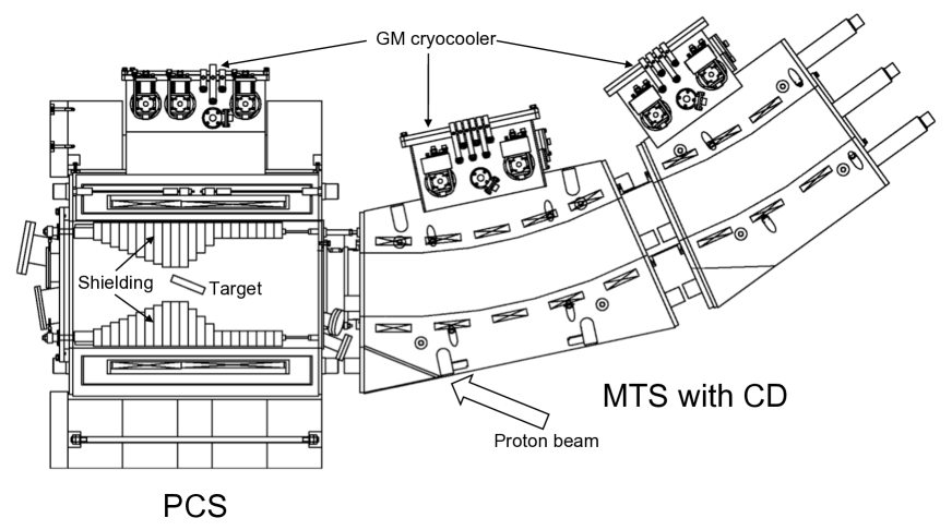
Figure 1: Layout of the MuSIC beamline showing the target surrounded by shielding and the pion capture solenoid (PCS). To the right are the two modules of five and three element coils, respectively, of the muon transport solenoid (MTS), covering an arc of $36^{\circ}$. Each coil in the MTS includes a correction dipole (CD). All superconducting coils are cooled with conduction cooling using Gifford–McMahon (GM) cryocoolers. The direction of the incoming proton beam is also indicated.

To reduce backgrounds from in particular neutrons and protons which will primarily be emitted in the forward (direction of initial proton beam) direction, backward-going pions are collected. Backward-going pions are captured by the PCS with a peak magnetic field of 3.5 T and focused towards the muon transport solenoid (MTS) via the graded magnetic field. The design parameters of the PCS are given in Table 1 [17].

The copper-stabilised NbTi superconducting coils are cooled using three GM cryocoolers which have a total cooling power of 4 W at the operating temperature of 4 K. Nuclear heating, mostly due to neutrons, was estimated using the MARS simulation [23, 24, 25, 26, 27]. The coil density was assumed to be 9 g$/$cm³ and the thickness of the stainless steel support structure of the coil was 10 mm. The total energy deposited at the solenoid coils including the support structure was about 0.6 W for a proton beam of 400 MeV and 1 $\mu$A. Given a static heat load of 1 W, the combined value is below the cryocoolers total cooling power.

Table 1: Design parameters of the pion capture solenoid (PCS), muon transport solenoid (MTS) and correction dipole (CD) magnets. The coil thickness for the PCS is 40 mm for upstream of 400 mm to increase the magnetic field. RRR is a residual-resistance ratio of superconductors used.

	PCS	MTS	CD
Conductor	Cu stabilised NbTi	Cu stabilised NbTi	Cu stabilised NbTi
Conductor diameter (mm)	1.2	1.2	1.2
Cu / NbTi	4	4	4
RRR (R293K / R10K)	$>$ 240	$>$ 150	$>$ 150
Coil diameter (mm)	900	480	460
Coil length (mm)	1 000	200	200
Coil thickness (mm)	35	30
Number of turns	30 000	4 000	528
Operation current (A)	145	145	115 (Bipolar)
Field (T)	3.5	2	0.04
Inductance (H)	400	124	0.04
Stored energy (MJ)	5	1.4
Quench back heater	1.2 mm Cu wire	1.3 mm Cu wire

The curved MTS is employed to preferentially select muons in the momentum region ($\sim 20-60$ MeV) low enough to be subsequently stopped in a target further downstream. In order to have a high transport efficiency for such muons, the solenoid has a large bore of 36 cm with an on-axis magnetic field of 2 T. A correction dipole (CD) magnetic field from $-0.04$ T to $+0.04$ T is applied in order to keep the trajectory of the low energy muons roughly centred and to filter out other particles. The CD magnetic field can be also used to select electric charges of muons in the beam coming to downstream. However, the covered arc of 36^∘ is not large enough to obtain good separation of charges, and therefore, contamination of oppositely charged particles in the beam, could not be fully eliminated, as mentioned later. The design parameters of the MTS and CD are given in Table 1.

4 Muon detection

The particles exiting the beam-pipe were a mixture of electrons and positrons, pions and muons of both charges and protons and neutrons, because of the short arc of 36^∘ coverage of the MTS. The challenge of this experiment is to measure the muon flux above such high backgrounds. Two methods were employed, the first of which measures electrons (and positrons) from muon decays and the second measures negatively charged muons. The first relies on measuring the decay time spectrum of the muon to identify and count their number by measuring a coincidence of a muon in one detector followed by an electron in a later detector. The second measures the muonic X-ray energy spectrum emitted by the negatively-charged muons captured by a nucleus. The experimental set-ups are given in the following.

4.1 Muon decay spectrum

A system to measure the muon flux was made by detecting electrons (and positrons) from muon decays. The correction magnetic field $B_{\rm CD}=-$0.04 T was set to primarily select positively charged muons. According to simulations (see Section 5), electrons made up about 74% of the beam with positrons the next most prevalent, making up about 10% of total population. The fraction of positive and negative muons was estimated to be about 5% and 0.5% respectively

An aluminium degrader, with height and width both of 400 mm, was optionally placed immediately after the beam exited the beam-pipe and magnet system. Thicknesses of 0.5, 1 and 5 mm were used in order to select different ranges of muon momentum. From simulations, the mean momentum for muons at the end of the beam-pipe and subsequently stopped were e.g. with no degrader and a 5 mm-thick degrader, $45.2\pm 0.2$ MeV and $66.1\pm 0.2$ MeV, respectively. After the degrader, a copper or magnesium stopping target was sandwiched between two sets of plastic scintillator counters. The first scintillator, S1, consisted of eight channels, with height and width of 30 mm and 380 mm and was 0.5 mm thick, in order to disturb the beam minimally. This counter was used to detect the passage of the initial muons. The second scintillator, S2, consisted of five channels, with height and width of 50 mm and 380 mm, and was of thickness 3.5 mm; this was used to detect electrons from the decay of a muon. The scintillators were wrapped in reflective mylar foils and black plastic sheets to prevent light leakage. Each scintillator strip had a wavelength-shifting fibre mounted on the back of it which was connected to a multi-pixel photon counter (MPPC) at each end. The signals from each pair of MPPCs were combined and amplified before being passed to the data acquisition (DAQ) system for processing. A schematic of the set-up is shown in Figure 2.

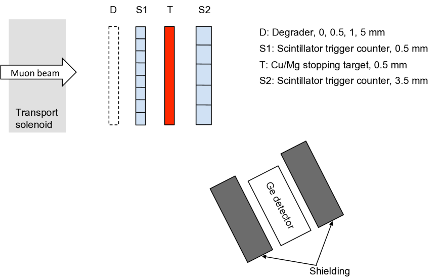
Figure 2: Schematic of the independent detection systems for measuring the muon flux. After 36^∘ arc of the muon beamline, the beam, including muons, exits the transport solenoid and optionally passes through an aluminium degrader, D. The beam then passes through a plastic scintillator trigger counter, S1, and a target, T, where muons are stopped. X-rays emitted by a captured muon dropping down orbital energy levels are detected in a germanium detector which is also shielded. Electrons arising from the decay of a muon are registered in another plastic scintillator, S2.

In order to trigger on muon decays, a “hit” recorded in S2 was required to occur 50 ns to 20 $\mu$s after the hit in S1. A hit in S1 was defined as a coincident signal in both MPPCs of a given scintillator strip where the signal value was at least 8 photons, set by a discriminator. A hit in S2 was given by a signal of at least 10 photons, higher than in S1 as electrons deposit more energy in the thick scintillators than slow muons in the thin scintillators. The time difference, $t$, between the signals in S1 and S2 was used for further analysis in order to reconstruct the muon decay time spectrum.

4.2 Muonic X-ray measurement

A complementary system to measure the negative muon flux was the use of a germanium detector to measure X-rays emitted by negatively charged muons as they drop down energy levels in a muonic atom after being captured by one of the nuclei in the target, T, shown in Figure 2. A stopping target was made of magnesium of 20 mm thickness, with height and width of 80 mm and 370 mm. The germanium detector is a planar type of Canberra GL0515R with a germanium crystal of an active diameter of 25.2 mm and depth of 15 mm. The cryostat window, made of beryllium, was 0.15 mm thick. To ensure low backgrounds from particles exiting the beam line and other secondary interactions, the detector was placed off axis by 25^∘ from the beam axis and a distance of 500 mm from the target. The CD magnetic field of $B_{\rm CD}=+0.04$ T was chosen to select negatively charged muons. This setup is also shown schematically in Figure 2.

Since the detector was not far from the proton target, the neutron flux at the detector location was very high. To reduce neutrons, the germanium detector was shielded with paraffin, cadmium, and lead blocks from outer to inner sides. The paraffin cylindrical shielding of 100 mm thickness was used to decelerate fast neutrons to thermal neutrons. The cadmium shielding of 2 mm thickness was used to absorb thermal neutrons followed by $\gamma$-ray emission. The lead shielding of 50 mm thickness was used to absorb $\gamma$-rays from cadmium and other $\gamma$-rays. Furthermore, it was found that characteristic X-rays from lead blocked the muonic $L_{\alpha}$ X-rays and the pionic X-rays from magnesium. Additional shielding, which consisted of cylindrical tubes of tin, copper and aluminium (outer to inner) were placed between the germanium detector and the lead shielding.

The signal output from the germanium detector was amplified and fed to a multi-channel analyser (MCA). The MCA was triggered by the muon stop logic signal formed by the beam hodoscopes. The energy calibration of the germanium detector was made by using a ¹³³Ba source.

5 Simulation

The experimental set up was simulated in order to aid the design of the detectors, to determine efficiencies and acceptances, and to compare to the data. Two codes were used to perform the simulation: G4Beamline [28] was used to simulate the hadron production and track particles through the beamline; and Geant4 [29] was used to simulate the detectors.

G4Beamline was used to simulate the bulk of the experiment: the initial proton beam; the pion capture system, including the target, capture solenoid, shielding and return yoke; and the transport system, bending magnets and beampipe sections. The position and momentum of all particles passing through the end of the beamline were recorded and used as input to the subsequent Geant4 simulation.

Geant4 is used to simulate the detector set-up shown in Figure 2. Using the output from G4Beamline, the particles pass through materials constituting the various detector components, interacting with them according to formulae for energy loss, emission spectra, etc.. A full optical simulation of photon production in the scintillators and detection in the MPPCs was performed. The QGSP_BERT_HP physics list in Geant4 was used to simulate hadronic interactions as this is designed to transport neutrons with energies as low as 20 MeV. The reconstruction and cuts described in Section 4 as well as the signal extraction described in Section 6 were performed on the simulated data as for the real data.

6 Analysis method

6.1 Analysis of muon lifetime

The distributions of $t$ are shown in Figure 3 for each of the five S2 channels for an example data sample (see [30] for other samples). Also shown is a fit, $N(t)$, to the data given by:

$$N(t)=N_{f}\exp\left(-\frac{t}{\tau_{f}}\right)+N_{s}\exp\left(-\frac{t}{\tau_{s}}\right)+N_{b1}\sin\left(2\pi\frac{t-\phi}{T}\right)+N_{b2}\,,$$ (7)

where $t$ is the time in ns. The four components correspond to the free decay of positive muons, $f$, the decay of negative muons in the stopping target, $s$, a sinusoidal background, $b1$, and a flat background, $b2$. The muon decays rates are parametrised with a scale factor, $N$, and a lifetime, $\tau$. The sinusoidal background term, which comes from beam particles (mostly electrons) directly hitting the counters, has a period, $T$, and a phase relative to the trigger time, $\phi$. It is due to the minor bunching of the protons in acceleration with RF frequency of the RCNP cyclotron. The flat background term is due to combinatorial background of beam particles which fake a signal. Known values of the lifetimes, $\tau_{f}=2\,196.9811\pm 0.0022$ ns [9] and, for a copper stopping target, the lifetime of a muonic atom of copper [31], $\tau_{s}=163.5\pm 1.0$ ns, were fixed in the fit. The value of $T$ was also fixed to $60\pm 5$ ns determined by fitting the background noise in a region where no signal is expected, i.e. high $t$. The time distribution for an example data sample, with a degrader thickness of 5 mm, is shown for each of the five S2 channels in Figure 3. The fit to the data with the function in Equation (7 ) is also shown. The fits to the data are reasonable with some distributions having values of $\chi^{2}$ per degree of freedom of about one as is the case for the first channel shown here. Channels 4 and 5 give consistently poor values, worse than channels from 1 to 3, and so are excluded from further analysis.

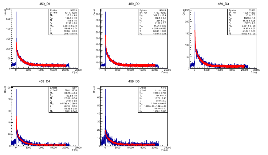
Figure 3: Time distribution for an example data sample, with a degrader thickness of 5 mm, for each of the five S2 channels. The fit to the data with the function in Equation (7) and the parameters extracted for each distribution are also shown.

The functions for the free decays of positive muons and decays of negative muons in a muonic atom of copper with parameters extracted in the fit to the data are then integrated in order to determine the number of muons in each sample. As a cross check of the method, simulated distributions were fit with the function in Equation (7) and the number of muons extracted. These values agreed with simply counting the number of real muons in the simulation.

The dead time of the DAQ system, due to it being busy, was calculated for each running configuration from the number of potential and good triggers. The potential triggers were those with a signal in the upstream scintillator and no corresponding signal downstream within the 50 ns veto window. A good trigger was defined as a potential trigger without the system being busy. The dead time varied from $38.43\pm 0.03$ % when no degrader was used to $15.05\pm 0.12$ % when a 5 mm-thick degrader was used. The decreasing dead time with increasing degrader thickness is to be expected due to the decrease in the overall rate of beam particles entering the detector system. In order to calculate the muon flux, the data were corrected for the dead time.

In order to extract a measured value, independent of the detector set-up, the muon flux was corrected for the detector acceptance and the MPPC efficiency. The detector acceptance was calculated with simulation by determining the fraction of muons which produced the signals described previously in the two scintillator detectors. The value was $A=79.6\pm 1.2$%. The efficiency of the MPPCs was determined using cosmic rays by placing the scintillator and MPPC system between a set of large scintillator paddles with the scintillation photons detected by photomultiplier tubes. By requiring a coincidence in the paddles above and below, the efficiency of an MPPC, accounting for the geometrical acceptance, was determined to be $\epsilon=0.431\pm 0.134$. The large uncertainty comes from the lack of stability over time and the differences for different MPPCs. Given the requirement in the measurement of signals in both MPPCs for a given scintillator strip, this gives an efficiency of $\epsilon^{2}=18.6\pm 11.6$%. The efficiency of the MPPC system is the dominant systematic uncertainty.

Other uncertainties considered were related to the fitting procedure and extraction of the integrated number of the electrons and positrons from muon decays, $N_{e}$ , in their time spectra. The lower bound on the fit and the binning of the data was varied. The uncertainty on the number of free positive muon decays was about 1.1%, where for negative muons decaying in copper, it was about 56%. The large uncertainty for the results of decays in copper arise due to the sensitivity of the fit at small times where the decays in copper are concentrated.

The total number of muons stopped in the target, $N_{\mu}$, measured by the decay electrons and positrons is given by

$$N_{\mu}={N_{e}\over{A\cdot\epsilon^{2}}}\,,$$ (8)

where $A$ and $\epsilon$ are the detector acceptance and the MPPC efficiency respectively. The data samples with the same degrader thickness give consistent results, demonstrating control of the analysis with time. The muon rate also decreases with increasing degrader thickness, consistent with the expectation. These two qualitative conclusions were observed for both free decays of positive muons and negative muons decaying in a muonic atom of copper.

6.2 Analysis of muonic X-ray measurement

The muonic X-ray measurements on magnesium were done for three data sets [32]. The list of the data sets is shown in Table 2, where different proton beam currents were used. The X-ray spectra for each data set are shown in Figure 4, where muonic $K_{\alpha}$ and $L_{\alpha}$ X-rays were measured together with pionic X-rays. The energy calibration was done using a ¹³³Ba source.

Table 2: Data sets for muonic X-ray measurements with different proton beam currents.

Data	Measurement	Proton beam	Muonic $K_{\alpha}$	Muonic $L_{\alpha}$
name	time (s)	current (pA)	X-ray events	X-ray events
		($I_{p}$)	($N_{2\rightarrow 1}$)	($N_{3\rightarrow 2}$)
data1	$1.0\times 10^{4}$	59	$23\pm 6$	$46\pm 13$
data2	$1.1\times 10^{4}$	134	$72\pm 12$	$141\pm 22$
data3	$1.0\times 10^{4}$	435	$212\pm 21$	$318\pm 48$

The muonic X-ray peaks were fit with a Gaussian and a constant background to obtain the total number of events of muonic X-rays. The energy dependence of the X-ray peak width was found from the measured data to be

$$\sigma=0.0196\sqrt{E({\rm keV})+57}\,.$$ (9)

The numbers of muonic X-ray events are summarised in Table 2.

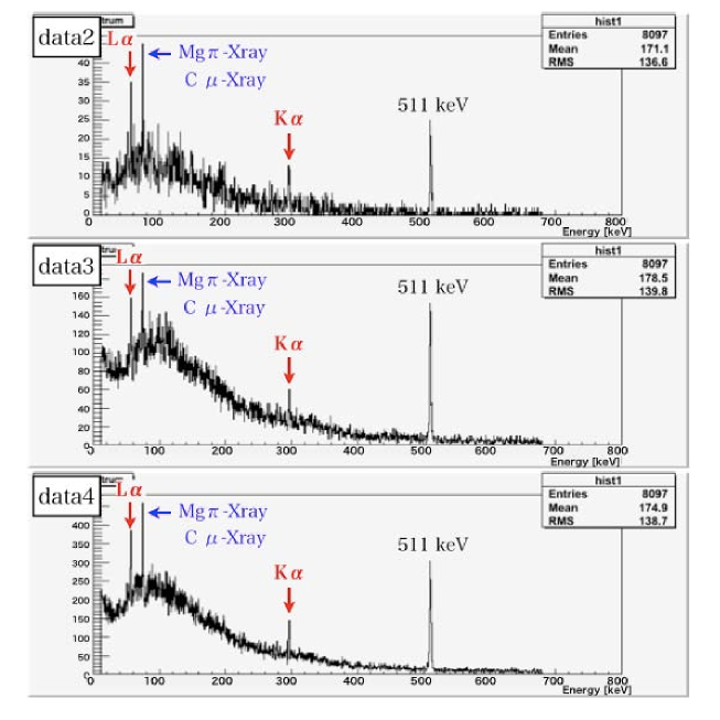
Figure 4: Muonic X-ray spectra for different data sets.

The total number of negatively charged muons stopped in the target, $N_{\mu}$, was determined using the following

$$N_{\mu^{-}}={N_{i\rightarrow j}\over P_{i\rightarrow j}\times(\Omega/4\pi)\times\varepsilon}\,,$$ (10)

where $N_{i\rightarrow j}$ and $P_{i\rightarrow j}$ are the number and the emission probability of the muonic X-ray in transition from the muonic atomic state of $i$ to that of $j$; $P_{i\rightarrow j}$ is known [34] and listed in Table 3. The quantity $(\Omega/4\pi)$ is the solid angle of the germanium detector and $\varepsilon$ is the efficiency of the germanium detector. Their combination, $\Omega_{D}=(\Omega/4\pi)\times\varepsilon$ can be estimated from Geant4 simulations taking into account the energy dependence of absorption by material and that of detection in germanium. The values $\Omega_{D}=(1.28\pm 0.05)\times 10^{-5}$ for $K_{\alpha}$ X-rays and $\Omega_{D}=(2.77\pm 0.12)\times 10^{-5}$ for $L_{\alpha}$ X-rays were obtained.

Table 3: Energy and emission probability for different muonic X-rays on magnesium.

Muonic X-ray	Energy	Probability
($i\rightarrow j$)	$E_{i\rightarrow j}$ (keV) [33]	$P_{i\rightarrow j}$ (%) [34]
$K_{\alpha}$ ($2\rightarrow 1$)	296.4	$(79.6\pm 0.7)$
$L_{\alpha}$ ($3\rightarrow 2$)	56.6	$(62.5\pm 0.7)$

The simulation was validated by the measurements with the standard calibration source of ¹³³Ba with its known absolute strength. The source was placed 200 mm away from the germanium detector. The comparison between the simulation and the measurement gave uncertainties of 2 % and 6 % for the reconstruction of the $K_{\alpha}$ and $L_{\alpha}$ X-rays.

7 Results and measurement of muon beam intensity

7.1 Results from muon lifetime analysis

The final number needed in order to extract the total muon flux is the number of muons which pass through the degrader, subsequently stopped and are measured in the detector system. The simulation started from the pion production was used to get the muon stopping distribution in the stopping target. Figure 5 shows the momentum distribution of muons stopped in the target from the simulation. From simulation, the probability of the muons stopping was determined to be at most $F_{s}=8$%, depending on the degrader thickness and includes both positive and negative muons.

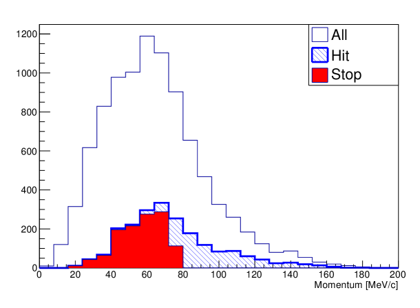
Figure 5: Momentum distributions for all muons in a beam (white), the muons hitting the trigger counters (blue) and those stopped in the target (red).

Given an expected beam design current of 1 $\mu$A, the final muon flux in muons per second is given by

$$J_{\mu}={N_{\mu}\over{I_{p}\cdot F_{s}\cdot D\cdot L}}\,,$$ (11)

where $I_{p}$ is the proton beam current in $\mu$A, $D$ is the duration of the run and $L$ is the live time, i.e. the dead time subtracted from 100%.

The data samples taken with different degrader thickness are consistent with each other and so averaging over these values gives a final flux of $J_{\mu}=(4.2\pm 1.1)\times 10^{8}$ muons s^-1 which corresponds to an efficiency for full beam power (400 W) of $J_{\mu}/W_{p}=(10.4\pm 2.7)\times 10^{5}$ muons s^-1 W^-1. This value is far in excess of any other muon source, i.e. is the by far the most efficient muon beam produced.

7.2 Results from X-ray measurements

From the three data sets with different proton beam currents, the muon beam intensity of negative muons, $J_{\mu^{-}}$ , was obtained to be

$$J_{\mu^{-}}={N_{\mu^{-}}\over{I_{p}\cdot F_{s}\cdot D\cdot L}}\,,$$ (12)

where $I_{p}$ is the proton beam current in $\mu$A and $D$ is the duration of the run and $L$ is the live time. $N_{\mu^{-}}$ is the total number of muons stopped in the target, given in Equation (10). The measurements of $K_{\alpha}$ and $L_{\alpha}$ X-rays were combined. For a maximum proton beam current of 1 $\mu$A at RCNP, a muon yield of $J_{\mu^{-}}=(3.6\pm 0.4)\times 10^{7}$ muons s^-1, which is the world’s highest, was obtained. The muon yield per beam power is $J/W_{p}=(9.0\pm 1.0)\times 10^{4}$ muons s^-1 W^-1, an improvement of about 1 000 over existing facilities. Geant simulations with QGSP_BERT give about $J_{\mu^{-}}=6.5\times 10^{7}$ muons s^-1, which is larger than the measured yield. This could be due to the hadron code in Geant simulations.

8 Summary

The world’s most efficient muon beam has been produced at the MuSIC facility in Osaka, Japan. The muon yield per beam power was measured to be (for $\mu^{+}$ and $\mu^{-}$) $(10.4\pm 2.7)\times 10^{5}$ muons s^-1 W^-1 and (for $\mu^{-}$ only) $(9.0\pm 1.0)\times 10^{4}$ muons s^-1 W^-1, over a factor of 1 000 higher than current facilities. Given a maximum beam power of 400 W, rates of about $4\times 10^{8}$ muons s^-1 are achievable. The increase in efficiency arises principally due to the use of a novel superconducting solenoid magnet system to capture pions produced at a target. This demonstration in increased efficiency will be utilised in future muon experiments in order to maximise the flux of muons and hence search for charged lepton flavour violation.

9 Acknowledgements

This work is supported in part by the Japan Society of the Promotion of Science (JSPS) KAKENHI Grant No. 25000004. The support of the Science and Technology Facilities Council, UK is acknowledged. M. Wing acknowledges the support of DESY and the Alexander von Humboldt Stiftung.

References

- [1] Y. Kuno and Y. Okada, Rev. Mod. Phys. 73 (2001) 151.
- [2] R.H. Bernstein and P.S. Cooper, Phys. Rept. 532 (2013) 27.
- [3] J. Adam et al. (MEG Collaboration), Phys. Rev. Lett. 110 (2013) 201801.
- [4] Y. Kuno (on behalf of the COMET Collaboration), Prog. Theo. Exp. Phys. (2013) 022C01.
- [5] R.J. Abrams et al. (Mu2e Collaboration), Mu2e Conceptual Design Report, Fermilab-TM-2545, arXiv:1211.7019 (2012).
- [6] A. Blondel et al., Research Proposal for an Experiment to Search for the Decay , arXiv:1301.6113 (2012).
- [7] D.M. Webber et al. (MuLan Collaboration), Phys. Rev. Lett. 106 (2011) 041803.
- [8] G.W. Bennett et al. (Muon Collaboration), Phys. Rev. D 73 (2006) 072003.
- [9] J. Beringer et al. (Particle Data Group), Phys. Rev. D 86 (2012) 010001 and 2013 partial update for the 2014 edition.
-
[10]
R.M. Carey et. al. (New Muon () Collaboration), see
lss.fnal.gov/archive/testproposal/0000/fermilab-proposal-0989.shtml - [11] N. Saito (J-PARC EDM Collaborations), AIP Conf. Proc. 1467 (2012) 45.
-
[12]
M.A. Palmer (Ed.), Muon Collider and Neutrino Factory Overview, ICFA Beam Dynamics Newsletter, 55 (2011)
http://icfa-usa.jlab.org/archive/newsletter/icfa_bd_nl_55.pdf - [13] S.J. Blundel, Contemporary Phys. 40 (1999) 175.
- [14] A. Yaouanc and P. Dalmas de Réotier, Muon Spin Rotation, Relaxation and Resonance: Applications to Condensed Matter, Oxford University Press (2011).
- [15] H. Daniel, Nucl. Instrum. Meth. B 3 (1984) 65.
- [16] M.K. Kubo et al., J. Radioanal. Nucl. Chem. 278 (2008) 777.
- [17] M. Yoshida et al., Superconducting Solenoid Magnets for the MuSIC Project, IEEE Trans. Appl. Supercond. 21 (2011) 1752.
- [18] R. Djilkibaev and V.M. Lobashev, Sov. J. Nucl. Phys. 49 (1989) 384.
- [19] R. Djilkibaev and V.M. Lobashev, The solenoid muon capture system for the MELC experiment, AIP Conf. Proc. 372 (1996) 53.
- [20] S. Geer, Phys. Rev. D 57 (1998) 6989.
- [21] T. Prokscha et al., Nucl. Instrum. Meth. A 595 (2008) 317.
- [22] I. Miura, The Research Center for Nuclear Physics Ring Cyclotron, in Proc. PAC1993, Washington DC, USA (1993) p.1650.
- [23] N.V. Mokhov, The Mars Code System User’s Guide, Fermilab-FN-628 (1995).
- [24] O.E. Krivosheev and N.V. Mokhov, MARS Code Status, Proc. Monte Carlo 2000 Conf., Lisbon (2000) p.943, Fermilab-Conf-00/181.
- [25] N.V. Mokhov, Status of MARS Code, Fermilab-Conf-03/053 (2003).
- [26] N.V. Mokhov et al., Recent Enhancements to the MARS15 Code, Fermilab-Conf-04/053 (2004).
- [27] http://www-ap.fnal.gov/MARS/
- [28] T.J. Roberts and D.M. Kaplan, G4Beamline Simulation Program for Matter-dominated Beamlines, in Proc. PAC2007, Albuquerque, New Mexico, USA (2007) p.3468.
-
[29]
S. Agostinelli et al., Nucl. Instrum. Meth. A 506 (2003) 250;
J. Allison et al., IEEE Trans. Nucl. Science 53 (2006) 270. -
[30]
S.L. Cook, PhD thesis, University College London (2014), available at
http://www.hep.ucl.ac.uk/theses/SamCook.pdf - [31] T. Suzuki, D.F. Measday and J.P. Roalsvig, Phys. Rev. C 35 (1987) 2212.
-
[32]
Y. Hino, Master thesis (in Japanese), Osaka University (2012), available at
http://www-kuno.phys.sci.osaka-u.ac.jp/papers/m-thesis/fy2012_hino_m-thesis.pdf - [33] A. Suzuki, Phys. Rev. Lett. 19 (1967) 18.
- [34] P. Vogel, Phys, Rev. A 22 (1980) 4.