Novel electric field effects on Landau levels in multi-Weyl semimetals

Abstract

Multi-Weyl semimetals(WSMs) have an anisotropic non-linear dispersion along a 2-D plane and a linear dispersion in an orthogonal direction. They have topological charge $`n$’ and are created when two or multiple Weyl points or nodes with nonzero net monopole charge are brought together onto a high-symmetry point. We study the perturbation corrections up to second order of such multi-WSMs in crossed electric($\mathcal{E}$) and magnetic (B) fields in the low electric field approximation. As a result, the first order correction lifts only n-fold degeneracy of the lowest Landau levels(LLs) while the higher Landau levels are modified due to the second order perturbation. We study the signatures of these corrections due to electric fields on the density of states (DOS) subjected to a magnetic field.

I Introduction

After graphene, Weyl semimetal(WSM) is another gapless system which is going to study at a rapid pace. WSM is a three dimensional analog of graphene where the low energy Hamiltonian has isotropic relativistic linear dispersion in k space (which obey the 3D Weyl equation) from accidental degenerate band touching points referred to as Weyl points. The electronic states around the Weyl points possess a nonzero Berry curvature, which gives rise to topological charge $\pm 1$ vafek14 . As a consequence, WSMs host topologically protected surface states in the form of open Fermi arcs terminating at the projections of bulk Weyl points (WPs) of opposite chirality. Other fascinating physical consequences of these Berry phases are exotic transport phenomena such as a large negative magnetoresistance due to chiral anomaly volovik86 ; volovik09 ; son13 . In recent angle-resolved photoemission spectroscopy(ARPES) and scanning tunneling microscopy(STM) experiments, several materials such as Cd₃As₂ neupane14 ; jeon14 ; liu14 ; borisenko14 ; he14 ; li15 ; moll15 , Na₃Bi liu14a ,NbAsxu15a , TaPxu15 ; xu16 , ZrTe₅ chen15 ; li16 and TaAs lv15 ; lv15a ; lv15b ; huang15a ; xu15b ; yang15 ; inoue16 have been identified as Weyl semimetals. Also, several attempts have been made on the realization of WSMs in artificial systems such as photonic crystals chen15a ; zhang15 ; dubcek15 ; lu15 ; lu16 .

In addition to above isotropic or single WSM, a new three-dimensional topological semimetals have been proposed in materials with certain point-group characterized by $C_{4,6}$ symmetries xu11 ; fang12 ; huang16 e.g. the double(triple)-Weyl semimetals have band touching points with quadratic(cubic) dispersions along $k_{x}-k_{y}$ plane and linear dispersion along $k_{z}$ direction. The double-Weyl nodes are protected by $C_{4}$ or $C_{6}$ rotation symmetry and its half-metallicity has been realized in the three-dimensional semimetal $\mathrm{HgCr_{2}Se_{4}}$ in the ferromagnetic phase, with a single pair of double-Weyl nodes along the z-direction guan15 . However, the material realization of triple-WSMs remains elusive. The double-Weyl node possesses a monopole(anti-monopole) charge of +2 (-2) and it shows double-Fermi arcs on the surface Brillouin zone(BZ) xu11 ; fang12 ; huang16 . Similarly, triple-Weyl node possesses a monopole(anti-monopole) charge of +3 (-3) and it shows triple-Fermi arcs on the surface BZ.

The single or isotropic-WSMs are predicted to have a fascinating response similar to graphene and 2D- WSM in crossed electric ($\mathcal{E}$) and magnetic fields (B) ming16 . These systems have topologically protected gapless Dirac or Weyl nodes with relativistic dispersion. This naturally induces Lorentz boosts in crossed electric ($\mathcal{E}$) and magnetic fields (B) luckose07 . As a consequence of Lorentz invariance of the Dirac equation, these problems can be solved exactly by choosing a reference frame in which the electric field vanishes as long as the drift velocity $v_{d}=\mathcal{E}/\mathrm{B}$ is smaller than the Fermi velocity($v_{F}$), which plays the role of an upper bound for the velocity as the speed of light c in relativity. This lifts the Landau levels(LLs) degeneracy. As a consequence, the LLs spacing is reduced and at a particular value of $\mathcal{E}/v_{F}\mathrm{B}$, the LLs get collapse ming16 ; luckose07 .

Our main contribution is to extend this mechanism for multi-WSMs(double and triple-WSMs). The double and triple-WSMs have non-Lorentz invariant physics due to quadratic and cubic dispersions respectively in $k_{x}-k_{y}$ plane and therefore their crossed electric and magnetic fields response cannot be solved exactly due to the absence of a reference frame in which the electric field vanishes. We, therefore, study this problem by perturbation theory up to second order corrections in electric fields as it has been discussed for multilayers graphene katsnelson13 . The rest of the paper is organized as follows. In Section II, we study the Landau level spectrum of the multi-Weyl semimetals in the presence of an in-plane uniform electric field. These problems have been well studied in 2-dimensional single layer graphene, 2-D WSMs and 3-dimensional single WSMs and type-II WSMsluckose07 ; peres07 ; goerbig09 ; morinari09 ; tchoumakov16 . In Section III, we study the response of multi-WSMs in crossed electric and magnetic fields by perturbation theory. We also calculate the density of states in crossed fields in Section IV. Finally, we make some concluding remarks in Section V.

II Landau levels formation in multi-Weyl semimetals

The non-interacting low energy effective Hamiltonian for a single multi-Weyl semimetals is given by ahn16 ; bitan15 ; lia16 ; ahna16 ,

$$H=\alpha_{n}[(\hat{p}_{-})^{n}\sigma_{+}+(\hat{p}_{+})^{n}\sigma_{-}]+\chi v_{z}\hat{p}_{z}\sigma_{z},$$ (1)

where $\sigma_{\pm}=\frac{1}{2}(\sigma_{x}\pm i\sigma_{y})$, $\hat{p}_{\pm}=\hat{p}_{x}\pm i\hat{p}_{y}$, and $\chi=\pm 1$ is the chilarity, $`n$’ represents monopole charge , $v_{z}$ is the Fermi velocity along $\hat{z}$ direction and $\alpha_{n}$ is the material dependent parameter, e.g. $\alpha_{1}$ and $\alpha_{2}$ are the Fermi velocity and inverse of the mass respectively for single and double WSMs. The energy spectrum of Eq.(1),

$$\epsilon_{s}(\mathbf{k})=s\sqrt{\alpha_{n}^{2}(\hbar k_{\parallel})^{2n}+\left(\hbar k_{z}v_{z}\right)^{2}},$$ (2)

where $s=\pm 1$ and $k_{\parallel}=\sqrt{k_{x}^{2}+k_{y}^{2}}$ is the momentum along $\hat{x}$-$\hat{y}$ plane. The density of states of such an anisotropic Hamiltonian is given by $g(\epsilon)\sim\epsilon^{2/n}$ ahn16 . In the presence of large external magnetic field, the Hamiltonian Eq.(1) form the Landau level spectrum Abrikosov98 ; Roy15 ; Chen16a . Under an external magnetic field B directed along $z$-axis, we make the usual Peierls substitution $\textbf{p}\rightarrow\textbf{p}+e\textbf{A}$ ($e>0$) in Hamiltonian Eq. (1) with the vector potential A. We choose A in the Landau gauge ($A_{y}=Bx$). Therefore, the Hamiltonian Eqn.$(1)$ transforms to

$$H=\left(\begin{array}[]{cc}v_{z}\hat{p}_{z}&\alpha_{n}\Bigl{(}\hat{p}_{x}-i(\hat{p}_{y}+eBx)\Bigr{)}^{n}\\ \alpha_{n}\Bigl{(}\hat{p}_{x}+i(\hat{p}_{y}+eBx)\Bigr{)}^{n}&-v_{z}\hat{p}_{z}\end{array}\right)$$ (3)

where $\hat{p}_{x,y,z}=-i\hbar\partial_{x,y,z}$. The time-independent Schrödinger equation $H\Psi=E_{m}\Psi$. Since the above Hamiltonian contain explicitly only x, we will look for the solutions of the usual form

$$\Psi=\Psi(x)e^{i\hbar(k_{y}y+k_{z}z)}$$ (4)

so that Eqn.$(3)$ transforms to

$$\left(\begin{array}[]{cc}\hbar v_{z}k_{z}&\alpha_{n}\Bigl{(}\hat{p}_{x}-i(\hbar{k}_{y}+eBx)\Bigr{)}^{n}\\ \alpha_{n}\Bigl{(}\hat{p}_{x}+i(\hbar{k}_{y}+eBx)\Bigr{)}^{n}&-\hbar v_{z}k_{z}\end{array}\right)\Psi(x)=E\Psi(x)$$ (7)

Let us now define a new variable $\quad u=\frac{(x+k_{y}l_{B}^{2})}{l_{B}}$ with $l_{B}=\sqrt{\hbar/(eB)}$ the magnetic length and introduce the annihilation and creation operators $\hat{a}=\frac{1}{\sqrt{2}}[u+\partial_{u}],\hat{a}^{{\dagger}}=\frac{1}{\sqrt{2}}[u-\partial_{u}]$ which satisfy the standard commutation relation $[\hat{a},\hat{a}^{{\dagger}}]=1$. Thus, Eqn.$(\ref{Big:eqn})$ becomes

$$\left(\begin{array}[]{cc}\hbar v_{z}k_{z}&(-i)^{n}\alpha_{n}(\sqrt{2}\frac{\hbar}{l_{B}})^{n}\hat{a}^{n}\\ (i)^{n}\alpha_{n}(\sqrt{2}\frac{\hbar}{l_{B}})^{n}[\hat{a}^{{\dagger}}]^{n}&-\hbar v_{z}k_{z}\end{array}\right)\Psi_{m}=$$ (10)

$$E_{m}\Psi_{m}$$

with Landau levels(LLs) spectrum for $m\geq n$

$$E_{m}^{0} = s\sqrt{m(m-1)...(m-n+1)(\omega)^{2n}\alpha_{n}^{2}+v_{z}^{2}\left(\hbar k_{z}\right)^{2}}$$

whereas for $m<n$

$$E_{0,1,2,...n}=\chi\hbar v_{z}k_{z}$$ (13)

with $\omega=\frac{\sqrt{2}\hbar}{l_{B}}$ and m is the Landau level index. Thus, it is clear from Eq.(13) that the lowest Landau levels(LLS) have n- degenerate chiral modes i.e. the lowest LLs for double and triple WSM have two and three fold degeneracy, respectively.

The normalized solutions for $m\geq n$ are

$$\Psi_{m,s=+}=\frac{1}{\sqrt{2}}\left(\begin{array}[]{c}(-i)^{n}b_{m}\psi_{m-n}\\ a_{m}\psi_{m}\end{array}\right)$$ (14)

$$\Psi_{m,s=-1}=\frac{1}{\sqrt{2}}\left(\begin{array}[]{c}-(-i)^{n}a_{m}\psi_{m-n}\\ b_{m}\psi_{m}\end{array}\right)$$ (15)

whereas for $m<n$

$$\Psi_{n}=\left(\begin{array}[]{c}0\\ \psi_{n}\end{array}\right)$$ (16)

where $a_{m}=\Bigl{(}1+\frac{v_{z}\hbar k_{z}}{E_{m}^{0}}\Bigr{)}^{1/2}$, $b_{m}=\Bigl{(}1-\frac{v_{z}\hbar k_{z}}{E_{m}^{0}}\Bigr{)}^{1/2}$ and $\psi_{m}$ are the usual normalized eigenfunctions of a free electron in a magnetic field

$$\psi_{m}=\frac{\sqrt{l_{B}}}{\sqrt{2^{m}m!\sqrt{\pi}}}e^{-u^{2}/2}H_{m}(u)$$ (17)

Here $H_{m}$ are Hermite polynomials.

III Energy levels in the presence of magnetic field and electric field

Let us assume that in addition to the magnetic field, one has an uniform electric field along the x direction. This add to the Hamiltonian a term of the form $-eV\textbf{1}=-e\mathcal{E}x\textbf{1}$ where V is the electric potential associated with the applied electric field $\textbf{E}=(\mathcal{E},0,0)$ and 1 is the $2\times 2$ unit matrix. Then the single particle Hamiltonian is given by

$$H=\left(\begin{array}[]{cc}v_{z}\hat{p}_{z}-e\mathcal{E}x&\alpha_{n}\Bigl{(}\hat{p}_{x}-i(\hat{p}_{y}+eBx)\Bigr{)}^{n}\\ \alpha_{n}\Bigl{(}\hat{p}_{x}+i(\hat{p}_{y}+eBx)\Bigr{)}^{n}&-v_{z}\hat{p}_{z}-e\mathcal{E}x\end{array}\right)$$ (18)

We try the wave function as $\Psi_{1,2}=\Psi_{1,2}(x)e^{i\hbar(k_{y}y+k_{z}z)}$. For n=1, the above $2\times 2$ Hamiltonian is an equivalent to a tilted WSMs ming16 and can be exactly solved for $\mathcal{E}/v_{F}B<1$ due to Lorentz invariant physics of the Hamiltonian. The corresponding eigenvalues are given by

$$E_{m}=\frac{1}{\gamma}\sqrt{v_{z}^{2}\hbar^{2}k_{z}^{2}+\frac{2eB\hbar}{\gamma}m\alpha_{1}^{2}}+\frac{\mathcal{E}}{B}\hbar k_{y}$$ (19)

where $\gamma=1/\sqrt{1-\beta^{2}}$, $\beta=\mathcal{E}/{\alpha_{1}B}$. Therefore, when $\mathcal{E}/{\alpha_{1}B}=1$, there is a complete collapse of the Landau Levels(LLs). The above Hamiltonian is not exactly soluble for topological charge $n>1$ due to the absence of a reference frame in which the electric field vanishes and therefore we solve the above problem for low electric field and high magnetic field such that Landau levels remain intact.

III.1 The zero order approximation

Let us introduce an another parameter $\lambda$

$$\lambda=\frac{e\mathcal{E}l_{B}}{\sqrt{2}}$$ (20)

such that $\lambda$ is always small with respect to the leading energy scale $2^{n/2}\hbar^{n}\alpha_{n}/l_{B}^{n}$ which holds at low electric field $\mathcal{E}$ . This validates the perturbation theory. Now, the Schrödinger equation (18) reads

$$\left(\begin{array}[]{cc}\hbar v_{z}k_{z}-\lambda(\hat{a}^{{\dagger}}+\hat{a})&(-i)^{n}2^{n/2}\frac{\hbar^{n}}{l_{B}^{n}}\alpha_{n}\hat{a}^{n}\\ (i)^{n}2^{n/2}\frac{\hbar^{n}}{l_{B}^{n}}\alpha_{n}[\hat{a}^{{\dagger}}]^{n}&-\hbar v_{z}k_{z}-\lambda(\hat{a}^{{\dagger}}+\hat{a})\end{array}\right)\Psi_{1,2}(x) = \tilde{E}_{m}\Psi_{1,2}(x)=(E_{m}-\frac{\mathcal{E}}{B}\hbar k_{y})\Psi_{1,2}(x)$$ (23)

When $\mathcal{E}$ is small, in the zeroth order approximation over $\lambda$ we have:

$$\hbar v_{z}k_{z}\psi_{1}+(-i)^{n}2^{n/2}\frac{\hbar^{n}}{l_{B}^{n}}\alpha_{n}[\hat{a}]^{n}\psi_{2} = (E_{m}-\frac{\mathcal{E}}{B}\hbar k_{y}){\psi}_{1}$$

$$(i)^{n}2^{n/2}\frac{\hbar^{n}}{l_{B}^{n}}\alpha_{n}[\hat{a}^{{\dagger}}]^{n}\psi_{1}-\hbar v_{z}k_{z}\psi_{2} = (E_{m}-\frac{\mathcal{E}}{B}\hbar k_{y}){\psi}_{2}$$

(We cannot neglect here $\frac{\mathcal{E}}{B}\hbar k_{y}$ because $\hbar k_{y}$ may be large.) Thus, we have the same Landau levels as without electric field just shifted by $\frac{\mathcal{E}}{B}\hbar k_{y}$.

         

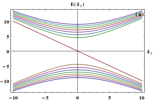
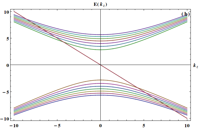
Figure 1: Landau levels spectrum for a single-Weyl semimetals for $k_{y}=0$ (a)obtained exactly for $\mathcal{E}=0$ and (b) obtained in perturbation theory to the second order in electric field for $\mathcal{E}=3.5$. Other parameters: B=5, $v_{z}$ =$1$, $\alpha_{2}=1$.

III.2 The first order correction

In the first order approximation, we have

$$\left(\begin{array}[]{cc}\hbar v_{z}k_{z}-\lambda(\hat{a}^{{\dagger}}+\hat{a})&(-i)^{n}2^{n/2}\frac{\hbar^{n}}{l_{B}^{n}}\alpha_{n}\hat{a}^{n}\\ (i)^{n}2^{n/2}\frac{\hbar^{n}}{l_{B}^{n}}\alpha_{n}[\hat{a}^{{\dagger}}]^{n}&-\hbar v_{z}k_{z}-\lambda(\hat{a}^{{\dagger}}+\hat{a})\end{array}\right)\Psi_{1,2}(x)=\tilde{E}_{m}\Psi_{1,2}(x)=(E_{m}-\frac{\mathcal{E}}{B}\hbar k_{y})\Psi_{1,2}(x)$$ (28)

One can easily see that the first-order term due to $\lambda$ vanishes for $m\geq n$. For $m<n$, we use degenerate first order perturbation theory capri and finds that there is the first order correction to the energy for $n\geq 2$. This correction is given by

$$\Phi_{m}^{\dagger}H^{\prime}\Phi_{m^{\prime}}=\tilde{E}_{m}^{(1)}\delta_{mm^{\prime}}{}$$ (29)

where $H^{\prime}=-\lambda(\hat{a}^{{\dagger}}+\hat{a})\mathbb{I}_{2\times 2}$ and $\Phi_{m}$ is a new basis which has been expressed in terms of original lowest Landau levels basis $\Psi_{m}$ by unitary transformation

$$\Phi_{m}=\sum_{m^{\prime}=0}^{n-1}a_{m^{\prime}}\Psi_{m^{\prime}}$$ (30)

where $a_{m^{\prime}}$ is the ampitude of $\Psi_{m^{\prime}}$ and summation is over lowest Landau levels (i.e.$m^{\prime}<n$). The matrices $\Omega$ formed from $\Psi_{p}^{\prime}H^{\prime}\Psi_{m}^{\prime}$ for double and triple-WSMs reduce to

$$\left(\begin{array}[]{cc}0&-\lambda\\ -\lambda&0\end{array}\right)=\Omega$$ (31)

and

$$\left(\begin{array}[]{ccc}0&-\lambda&0\\ -\lambda&0&-\sqrt{2}\lambda\\ 0&-\sqrt{2}\lambda&0\end{array}\right)=\Omega$$ (32)

respectively which have eigenvalues

$$\tilde{E}_{m}^{(1)}=\pm\lambda;$$

$$\tilde{E}_{m}^{(1)}=0,\pm\sqrt{3}\lambda$$ (33)

for double and triple-WSMs respectively. Therefore, in the presence of electric field $\mathcal{E}$, the n-fold degeneracy of chiral lowest LLs is lifted.

III.3 The second order approximation

We have already seen that the first-order term in $\mathcal{E}$ in powers of $\lambda$ vanishes for $m\geq n$. Therefore, we look at the second-order term

$$\tilde{E}_{m,s}^{(2)}=\lambda^{2}\sum_{k\neq m,s^{\prime}}\frac{1}{E_{m,s}^{(0)}-E_{k,s^{\prime}}^{(0)}}|\Psi_{m,s}^{\dagger}(\hat{a}^{{\dagger}}+\hat{a})\Psi_{k,s^{\prime}}|^{2}$$ (34)

where s, $s^{\prime}$ denotes the band index.

First, we consider the case $m\geq n$ for which Eq. (34) can be rewritten as

$$\tilde{E}_{m}^{(2)} = \frac{\lambda^{2}}{4}\Bigl{(}\frac{1}{E_{m}^{(0)}-E_{m+1}^{(0)}}[a_{m+1}a_{m}\sqrt{m+1}+b_{m+1}b_{m}\sqrt{m-n+1}]^{2}$$ (35)

$$+\frac{1}{E_{m}^{(0)}-E_{m-1}^{(0)}}[a_{m}a_{m-1}\sqrt{m}+b_{m}b_{m-1}\sqrt{m-n}]^{2}$$

$$+\frac{1}{E_{m}^{(0)}+E_{m+1}^{(0)}}[a_{m}b_{m+1}\sqrt{m+1}-a_{n+1}b_{n}\sqrt{m-n+1}]^{2}$$

$$+\frac{1}{E_{m}^{(0)}+E_{m-1}^{(0)}}[a_{m}b_{m-1}\sqrt{m}-a_{m-1}b_{m}\sqrt{m-n}]^{2}\Bigr{)}$$

$$=\frac{\lambda^{2}}{4}\zeta_{m}$$

with

$$\zeta_{m} = \frac{2}{\theta_{1}}\Bigl{[}\{2(m+1)-n\}E_{m}^{0}+2n\hbar v_{z}k_{z}+\{2(m+1)-n\}\frac{(\hbar v_{z}k_{z})^{2}}{E_{m}^{0}}$$ (36)

$$+\frac{2}{E_{m}^{0}}(m+1)m(m-1)....(m-n+1)\omega^{2n}\alpha_{n}^{2}\Bigr{]}$$

$$\frac{2}{\theta_{2}}\Bigl{[}(2m-n)E_{m}^{0}+2n\hbar v_{z}k_{z}+(2m-n)\frac{(\hbar v_{z}k_{z})^{2}}{E_{m}^{0}}$$

$$+\frac{2}{E_{m}^{0}}m(m-1)....(m-n)\omega^{2n}\alpha_{n}^{2}\Bigr{]}$$

where $\theta_{1}=(E_{m}^{0})^{2}-(E_{m+1}^{0})^{2}=-nm(m-1)(m-2)....(m-n+2)\omega^{2n}\alpha_{n}^{2}$ and $\theta_{2}=(E_{m}^{0})^{2}-(E_{m-1}^{0})^{2}=n(m-1)(m-2)....(m-n+2)(m-n+1)\omega^{2n}\alpha_{n}^{2}$.

In particular, for a single WSMs case ($n=1$), the second order energy correction

$$\tilde{E}_{m}^{(2)} = -\frac{1}{4}\beta^{2}[2E_{m}^{0}+\frac{m}{E_{m}^{0}}(\alpha_{1}^{2}\omega^{2})]$$ (37)

$$=-\frac{1}{2}\beta^{2}E_{m}^{0}-\frac{1}{2}\frac{m}{E_{m}^{0}}(\hbar eB)\alpha_{1}^{2}\beta^{2}$$

         

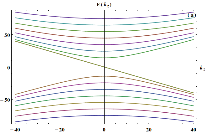
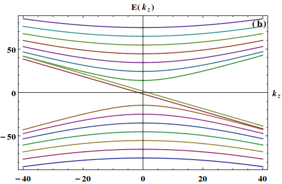
Figure 2: Landau levels spectrum for double-Weyl semimetals for $k_{y}=0$ (a) obtained exactly for $\mathcal{E}=0$ and (b) obtained in perturbation theory to the second order in the electric field for $\mathcal{E}=5$. Other parameters: B=5, $v_{z}$ =$1$, $\alpha_{2}=1$.

         

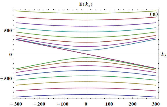
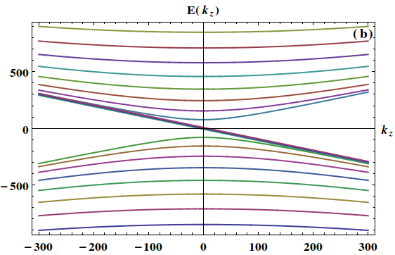
Figure 3: Landau levels spectrum for triple-Weyl semimetals for $k_{y}=0$ (a)obtained exactly for $\mathcal{E}=0$ and (b)obtained in perturbation theory to the second order in the lectric field for $\mathcal{E}=25$. Other parameters: B=5, $v_{z}$ =$1$, $\alpha_{2}=1$.

Therefore, the modified energy

$$E_{m} = E_{m}^{0}-\frac{1}{2}\beta^{2}E_{m}^{0}-\frac{1}{2}\frac{m}{E_{m}^{0}}(\hbar eB)\alpha_{1}^{2}\beta^{2}+\frac{\mathcal{E}}{B}\hbar k_{y}$$ (38)

$$\approx\frac{1}{\gamma}E_{m}^{0}-\frac{1}{2}\frac{m}{E_{m}^{0}}(\hbar eB)\alpha_{1}^{2}\beta^{2}+\frac{\mathcal{E}}{B}\hbar k_{y}$$

where we have taken $\gamma=1/\sqrt{1-\beta^{2}}\approx 1/(1-\frac{1}{2}\beta^{2})$ at low $\beta$ in above equation. This energy agrees with exact results for type-II WSMs or tilted single WSMs in ref.tchoumakov16 .

$$E_{m}(k_{z})=\frac{1}{\gamma}\sqrt{v_{z}^{2}\hbar^{2}k_{z}^{2}+\frac{2eB\hbar}{\gamma}m\alpha_{1}^{2}}+\frac{\mathcal{E}}{B}\hbar k_{y}$$ (39)

Similarly, we can show that Landau levels spectrum of other multi WSMs gets modified in the presence of electric field. For double-WSMs, the second order energy correction

$$\tilde{E}_{m}^{(2)} = \lambda^{2}\Bigl{[}-\frac{(2m-1)}{2E_{m}^{0}}+\frac{\hbar v_{z}k_{z}}{\omega^{4}\alpha_{2}^{2}m(m-1)}\Bigr{]}$$ (40)

and for triple-WSMs,we have second order energy correction

$$\tilde{E}_{m}^{(2)} = \lambda^{2}\Bigl{[}\frac{(E_{m}^{0})^{2}+(\hbar v_{z}k_{z})^{2}}{3E_{m}^{0}\omega^{6}\alpha_{3}^{2}m(m-2)}-\frac{2(m-1)}{3E_{m}^{0}}$$ (41)

$$+\frac{2\hbar v_{z}k_{z}}{m(m-1)(m-2)\omega^{6}\alpha_{3}^{2}}\Bigr{]}$$

Therefore, the corresponding modified energies for double WSMs is

$$E_{m} = E_{m}^{0}+\lambda^{2}\Bigl{[}-\frac{(2m-1)}{2E_{m}^{0}}+\frac{\hbar v_{z}k_{z}}{\omega^{4}\alpha_{2}^{2}m(m-1)}\Bigr{]}+\frac{\mathcal{E}}{B}\hbar k_{y}$$

and for triple-WSMs, the modified energy dispersion

$$E_{m} = E_{m}^{0}+\lambda^{2}\Bigl{[}\frac{(E_{m}^{0})^{2}+(\hbar v_{z}k_{z})^{2}}{3E_{m}^{0}\omega^{6}\alpha_{3}^{2}m(m-2)}-\frac{2(m-1)}{3E_{m}^{0}}$$ (43)

$$+\frac{2\hbar v_{z}k_{z}}{m(m-1)(m-2)\omega^{6}\alpha_{3}^{2}}\Bigr{]}+\frac{\mathcal{E}}{B}\hbar k_{y}$$

For m$<$n, we use degenerate perturbation theory(Rayleigh-Schrödinger solution)capri and and show it easily that the second order correction vanishes due to the cancellation from positive and negative energy bands of higher Landau levels. Therefore, the modified lowest LLs energy dispersion due to the first and second order corrections.

$$E_{m}=-\hbar k_{z}v_{z}+\frac{\mathcal{E}}{B}\hbar k_{y}-\lambda\mathrm{EV}[\Omega]$$ (44)

where EV$(\Omega)$ represents the eigenvalues of $\Omega$.

Thus, energy spectrum of lowest LLs for double and triple-WSMs are $-\hbar k_{z}v_{z}+\frac{\mathcal{E}}{B}\hbar k_{y}\pm\lambda$ and $-\hbar k_{z}v_{z}+\frac{\mathcal{E}}{B}\hbar k_{y}$, $-\hbar k_{z}v_{z}+\frac{\mathcal{E}}{B}\hbar k_{y}\pm\sqrt{3}\lambda$ respectively. Therefore, the n-fold degeneracy of lowest LLs is lifted due to the in-plane electric field $\mathcal{E}$ . The Eqns. (LABEL:eqn_dwsms), (43) and (34) are the modified energy spectrum of LLs and are our main results of the paper. The Landau levels spectrum for single, double and triple-WSMs with and without in-plane electric field are shown in Fig(1), Fig.(2) and Fig.(3) respectively. We have shown the Landau levels spectrum only near left chiral Weyl point. A similar LL spectrum can be easily obtained for right chiral Weyl point. It is clearly seen from Fig.(1 (b)), Fig.(2(b)) and Fig.(3(b)) that lowest Landau levels splits in the presence of $\mathcal{E}$ while it is unaffected without $\mathcal{E}$, see Fig.(1 (a)), Fig.(2(a)) and Fig.(3(a)). However, there is always n number of chiral lowest LLs cut the zero energy which can be substantiated by the fact that in zero magnetic fields the topological charge of the Weyl nodes is $\pm n$ (the degeneracy of the zero LLs). Thus, the lowest LLs in double and triple WSMs cuts the zero energy along momentum $k_{z}$ at $\pm\lambda/{\hbar v_{z}}$ and 0, $\pm\sqrt{3}\lambda/{\hbar v_{z}}$ respectively. This LLs splitting modifies the density of states(DOS) which could be observed in quantum oscillations experiments. Next, we discuss the DOS of the multi-WSMs with and without electric fields and their physical consequences.

IV Density of states

The density of states(DOS) governs the pattern of quantum oscillation measurements (through Shubnikov-de Haas effect or De Haas-van Alphen effect) of all transport and thermodynamic quantities lia16 ; pippard89 ; behnia11 . In the presence of high magnetic fields, the energy dispersion of multi-WSMs in the plane perpendicular to B is completely suppressed while it is still dispersive along the direction of the applied magnetic field. Thus the magnetic field step down the dimension of the system and the WSM in the external magnetic field can be visualized as a collection of one-dimensional systems with multiple subbands due to Landau levels. The DOS of multi-WSMs can be worked out by the following definition,

$$D(\varepsilon)=\frac{1}{2\pi l_{B}^{2}}\sum_{m}\int_{-\infty}^{+\infty}\frac{dk_{z}}{2\pi}\,\delta[E_{m}^{0}(k_{z})-\varepsilon],$$ (45)

where $m$ labels Landau level index, $k_{z}$ is the conserved momentum of the one-dimensional conducting channel along the B direction and $l_{B}$ is the magnetic length.

The DOS for multi- WSM in the absence of in-plane electric field $\mathcal{E}$ can be obtained analytically. Let us first consider the dispersion for a single WSM

$$E_{m}^{0}(k_{z})=\sqrt{\hbar^{2}v_{z}^{2}k_{z}^{2}+m\omega^{2}\alpha_{1}^{2}},$$ (46)

In such a system, each m$\geq$1 LLs crosses the Fermi energy $\varepsilon$ twice at critical momentum $k_{zc}=\pm\sqrt{\varepsilon^{2}-m\omega^{2}\alpha_{1}^{2}}/(\hbar v_{z})$, whereas the $m=0$ LL only cuts the Fermi energy once, at $k_{z}=-\varepsilon/(\hbar v_{z})$. Therefore, the DOS for this single WSM is given by

$$D(\varepsilon)=D_{0}\left[1+\sum_{m\geq 1}\frac{2\varepsilon\,\Theta(\varepsilon-\sqrt{m}\omega\alpha_{1})}{\sqrt{\varepsilon^{2}-m\omega^{2}\alpha_{1}^{2}}}\right],$$ (47)

where $D_{0}=1/(4\pi^{2}l_{B}^{2}\hbar v_{z})$ and $\Theta(x)$ is the Heaviside Theta function.

Similarly, the DOS for double WSM and triple WSMs can be obtainded analytically by the above same arguments. The DOS for double-WSM is given by

$$D(\varepsilon)=D_{0}\left[2+\sum_{m\geq 2}\frac{2\varepsilon\,\Theta(\varepsilon-\sqrt{m(m-1)}\omega^{2}\alpha_{2})}{\sqrt{\varepsilon^{2}-m(m-1)\omega^{4}\alpha_{2}^{2}}}\right],$$ (48)

and for triple-WSM

$$D(\varepsilon)=D_{0}\left[3+\sum_{m\geq 3}\frac{2\varepsilon\,\Theta\left[\varepsilon-\sqrt{m(m-1)(m-2)}\omega^{3}\alpha_{3}\right]}{\sqrt{\varepsilon^{2}-m(m-1)(m-2)\omega^{6}\alpha_{3}^{2}}}\right],$$ (49)

where the numbers 2 and 3 in Eqns.(48) and (49) accounted for the two-fold and three-fold degeneracy of the lowest LLs respectively.

                   

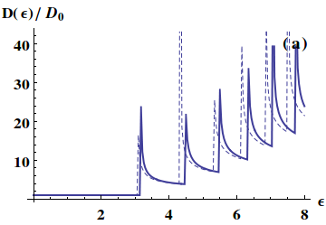
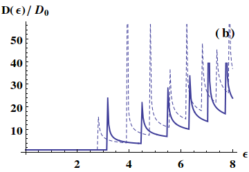
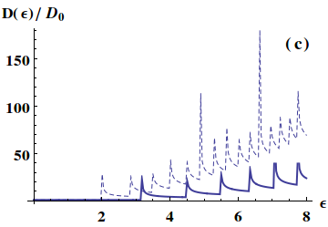
Figure 4: DOS for Landau levels in a single-WSM, renormalized by $D_{0}$ when (a) $\mathcal{E}=1$ (b) $\mathcal{E}=2$ and (c) $\mathcal{E}=3.5$ respectively. Dark and dotted plots shows the DOS without and with electric fields. Other parameters: B=5, $v_{z}$ =$1$, $\alpha_{1}=1$.

                   

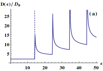
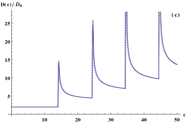
Figure 5: DOS for Landau levels in a double-WSM, renormalized by $D_{0}$ when (a) $\mathcal{E}=3$ (b) $\mathcal{E}=4$ and (c) $\mathcal{E}=5$ respectively. Dark and dotted plots shows the DOS without and with electric fields. Other parameters: B=5, $v_{z}$ =$1$, $\alpha_{1}=1$.

                   

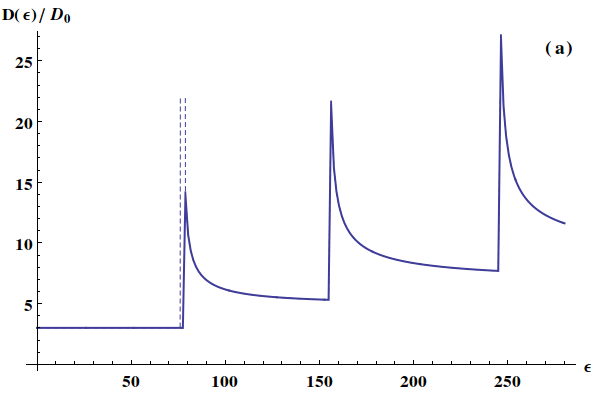
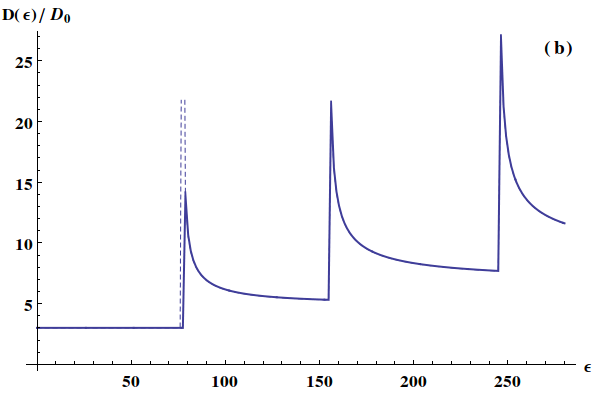
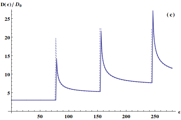
Figure 6: DOS for Landau levels in a triple-WSM, renormalized by $D_{0}$ when (a) $\mathcal{E}=5$ (b) $\mathcal{E}=10$ and (c) $\mathcal{E}=25$ respectively. Dark and dotted plots shows the DOS without and with electric fields. Other parameters: B=5, $v_{z}$ =$1$, $\alpha_{1}=1$.

In the presence of an in-plane electric field $\mathcal{E}$ along the x-direction, the DOS cannot be calculated analytically. Therefore, we compute it numerically using Eq.(45) and display in Fig.(4), Fig.(5) and Fig.(6) with increasing values of the electric field for single, double and triple-WSMs respectively. The magnetic oscillations have a sawtooth appearance originating from the $k_{z}$ dispersion of higher Landau levels (i.e. $m\geq n$). The peaks correspond to the spacing of the singularities which go like $B^{(}n/2)_{eff}$ where $B_{eff}$ is the effective or reduced effective magnetic field due to the electric field $\mathcal{E}$. In the case of single-WSMs, $B_{eff}$ is reduced strongly compared to the bare applied magnetic field $B$ along z-direction whereas it has a minor modifications for the case of double and triple-WSMs. As a result, a considerable shift of peaks towards low $\varepsilon$ are observed with increasing electric field $\mathcal{E}$ in the case for single-WSMs whereas there is a minor change in shift of peaks towards low $\varepsilon$ are observed for the double and triple-WSMs case. In the case of single-WSM, the LLs becomes closer and closer with increasing $\mathcal{E}$ and at the critical value $\mathcal{E}_{c}=v_{F}\mathrm{B}$, it collapses in the plane perpendicular direction to B while it is still dispersive along B. The corresponding DOS squeezes with the electric field and at a critical value $\mathcal{E}_{c}$, it reaches a constant value which corresponds to DOS of the one-dimension dispersion along the z-direction. For double and triple-WSMs, there are no such modifications in their DOS with $\mathcal{E}$ due to the non-collapse of the LLs and therefore, their DOS show small changes with $\mathcal{E}$. Further for lowest LLs (i.e. $m<n$), we observe that there is no change of the plateau in DOS at low energy $\epsilon$ due to the lifting of the degeneracy of their lowest LLs in the case of double and triple-WSMs. Since the degeneracy of lowest Landau level in the presence of in-plane electric field are symmetrically shifted about its lowest Landau levels energy $-\hbar v_{z}k_{z}$ in case of double and triple-WSMs. Therefore, when we add contributions from these shifted lowest Landau levels, it density of states(DOS) remains constants. These changes of DOS of multi-WSMs with $\mathcal{E}$ could be detected in angle-resolved quantum oscillations. e.g. the above features of DOS could be reflected in the specific heat and magnetization.

V Conclusion

In conclusion, we summarize the main findings of the present manuscript. We have analyzed a perturbative study of a multi-WSMs in crossed electric and magnetic fields in low electric field approximation. This problem cannot be exactly solved for monopole charge $n>1$ due to the absence of a reference frame in which the electric field vanishes. Therefore, we have calculated energy corrections up to second order. The main consequences of this electric field $\mathcal{E}$ are the n-fold degeneracy of the lowest Landau levels is lifted while the higher one remain unaffected due to the first order correction in electric field $\mathcal{E}$. The higher Landau levels have corrections due to the second order perturbation in electric field $\mathcal{E}$ while lowest Landau levels remain unaffected. We have compared the density of states of multi-WSMs system for both the absence and presence of the electric field. The lowest LLs (i.e. m$<$n)have no change of plateau in DOS at low energy $\epsilon$ in the case of double and triple-WSMs even with the lifting of the degeneracy of lowest LLs with electric field $\mathcal{E}$. Further, the higher LLs( m$\geq$ n) contribute to the considerable amount of shift of peaks towards low energy $\epsilon$ with increasing electric field $\mathcal{E}$ for the case of a single-WSM while it has a little shift of peaks for double and triple WSMs case. This changes in DOS can be directly tested in angle-resolved quantum oscillation measurements in the future.

VI Acknowledgements

We acknowledge helpful discussions with Debanand Sa, N. S. Vidhyadhiraja and Daniel Yumnam. This work is supported by Science and Engineering Research Board (SERB), India for the SERB National Post doctoral Fellowship. I would like to thank JNCASR for the facilities for this work.

References

References

• (1) O.Vafek and A.Vishwanath, Annual Review of Condensed Matter Physics 5, 83 (2014).
• (2) G. E. Volovik, JETP Lett, 43 9, (1986).
• (3) G. E. Volovik, The Universe in a Helium Droplet, Oxford University Press New York, (2009).
• (4) D. T. Son and B. Z. Spivak, Phys. Rev. B 88, 104412 (2013).
• (5) Madhab Neupane, Su-Yang Xu, Raman Sankar, Nasser Alidoust, Guang Bian, Chang Liu, Ilya Belopolski, Tay-Rong Chang, Horng-Tay Jeng, Hsin Lin, Arun Bansil, Fangcheng Chou and M. Zahid Hasan, Nat. Commun. 5, 3786 (2014).
• (6) Sangjun Jeon, Brian B. Zhou, Andras Gyenis, Benjamin E. Feldman, Itamar Kimchi, Andrew C. Potter, Quinn D. Gibson, Robert J. Cava, Ashvin Vishwanath and Ali Yazdani, Nat. Mater. 13, 851 (2014).
• (7) Z. K. Liu, J. Jiang, B. Zhou, Z. J. Wang, Y. Zhang, H. M. Weng, D. Prabhakaran, S-K. Mo, H. Peng, P. Dudin, T. Kim, M. Hoesch, Z. Fang, X. Dai, Z. X. Shen, D. L. Feng, Z. Hussain and Y. L. Chen, Nat. Mater. 13, 677 (2014).
• (8) Sergey Borisenko, Quinn Gibson, Danil Evtushinsky, Volodymyr Zabolotnyy, Bernd BΓΌchner, and Robert J. Cava, Phys. Rev. Lett. 113, 27603 (2014).
• (9) L. P. He, X. C. Hong, J. K. Dong, J. Pan, Z. Zhang, J. Zhang, and S. Y. Li, Phys. Rev. Lett. 113, 246402 (2014).
• (10) Cai-Zhen Li, Li-Xian Wang, Haiwen Liu, Jian Wang, Zhi-Min Liao and Da-Peng Yu, Nat. Commun. 6, 10137 (2015).
• (11) Philip J. W. Moll, Nityan L. Nair, Toni Helm, Andrew C. Potter, Itamar Kimchi, Ashvin Vishwanath and James G. Analytis, Nature 535, 266 (2016).
• (12) Z. K. Liu, B. Zhou, Y. Zhang, Z. J. Wang, H. M. Weng, D. Prabhakaran, S. K. Mo, Z. X. Shen, Z. Fang, X. Dai, Z. Hussain, Y. L. Chen, Science 343, 864 (2014).
• (13) Su-Yang Xu, Nasser Alidoust, Ilya Belopolski, Zhujun Yuan, Guang Bian, Tay-Rong Chang, Hao Zheng, Vladimir N. Strocov, Daniel S. Sanchez, Guoqing Chang, Chenglong Zhang, Daixiang Mou, Yun Wu, Lunan Huang, Chi-Cheng Lee, Shin-Ming Huang, BaoKai Wang, Arun Bansil, Horng-Tay Jeng, Titus Neupert, Adam Kaminski, Hsin Lin, Shuang Jia and M. Zahid Hasan, Nat. Phys. 111, 748 (2015).
• (14) Su-Yang Xu, Ilya Belopolski, Daniel S. Sanchez, Chenglong Zhang, Guoqing Chang, Cheng Guo, Guang Bian, Zhujun Yuan, Hong Lu, Tay-Rong Chang, Pavel P. Shibayev, Mykhailo L. Prokopovych, Nasser Alidoust, Hao Zheng, Chi-Cheng Lee, Shin-Ming Huang, Raman Sankar, Fangcheng Chou, Chuang-Han Hsu, Horng-Tay Jeng, Arun Bansil, Titus Neupert, Vladimir N. Strocov, Hsin Lin3, Shuang Jia and M. Zahid Hasan, Sci. Adv. 1, e1501092 (2015).
• (15) N. Xu, H. M. Weng, B. Q. Lv, C. E. Matt, J. Park, F. Bisti, V. N. Strocov, D. Gawryluk, E. Pomjakushina, K. Conder, N. C. Plumb, M. Radovic, G. AutΓ¨s, O. V. Yazyev, Z. Fang, X. Dai, T. Qian, J. Mesot, H. Ding and M. Shi, Nat. Commun. 7, 11006 (2016).
• (16) R. Y. Chen, S. J. Zhang, J. A. Schneeloch, C. Zhang, Q. Li, G. D. Gu and N. L. Wang, Phys. Rev. B 92, 075107 (2015).
• (17) Qiang Li, Dmitri E. Kharzeev, Cheng Zhang, Yuan Huang, I. PletikosiΔ‡, A. V. Fedorov, R. D. Zhong, J. A. Schneeloch, G. D. Gu and T. Valla, Nat. Phys. 12, 550 (2016).
• (18) B. Q. Lv, S. Muff, T. Qian, Z. D. Song, S. M. Nie, N. Xu, P. Richard, C. E. Matt, N. C. Plumb, L. X. Zhao, G. F. Chen, Z. Fang, X. Dai, J. H. Dil, J. Mesot, M. Shi, H. M. Weng and H. Ding Phys. Rev. Lett. 115, 217601 (2015).
• (19) B. Q. Lv, H. M. Weng, B. B. Fu, X. P. Wang, H. Miao, J. Ma, P. Richard, X. C. Huang, L. X. Zhao, G. F. Chen, Z. Fang, X. Dai, T. Qian and H. Ding, Phys. Rev. X 5, 031013 (2015).
• (20) B. Q. Lv, N. Xu, H. M. Weng, J. Z. Ma, P. Richard, X. C. Huang, L. X. Zhao, G. F. Chen, C. E. Matt, F. Bisti, V. N. Strocov, J. Mesot, Z. Fang, X. Dai, T. Qian, M. Shi and H. Ding, Nat. Phys. 11, 724 (2015).
• (21) S. M. Huang, S.Y. Xu, I. Belopolski, C. C. Lee, G. Chang, B. Wang, N. Alidoust, G. Bian, M. Neupane, C. Zhang, S. Jia, A. Bansil, H. Lin and M. Z. Hasan, Nat. Commun. 6, 7373 (2015).
• (22) S. Y. Xu, I. Belopolski1, N. Alidoust, M. Neupane, G. Bian, C. Zhang, R. Sankar, G. Chang, Z. Yuan, C. C. Lee, S. M. Huang, H. Zheng, J. Ma, D. S. Sanchez, B. Wang, A. Bansil, F. Chou, P. P. Shibayev1, H. Lin, S. Jia, M. Z. Hasan, Science 349, 613 (2015).
• (23) L. X. Yang, Z. K. Liu, Y. Sun, H. Peng, H. F. Yang, T. Zhang, B. Zhou, Y. Zhang, Y. F. Guo, M. Rahn, D. Prabhakaran, Z. Hussain, S.-K. Mo, C. Felser, B. Yan and Y. L. Chen, Nat. Phys. 11, 728 (2015).
• (24) H. Inoue, A. Gyenis, Z. Wang, J. Li, S. W. Oh1, S. Jiang, N. Ni, B. A. Bernevig, A. Yazdani, Science 351 1184 (2016).
• (25) W. J. Chen, M. Xiao, C. T. Chan, arXiv:1512.04681 (2015).
• (26) Dan-Wei Zhang, Shi-Liang Zhu and Z. D. Wang Phys. Rev. A 92, 013632 (2015).
• (27) Tena Dubček, Colin J. Kennedy, Ling Lu, Wolfgang Ketterle, Marin SoljačiΔ‡ and Hrvoje Buljan, Phys. Rev. Lett. 114, 225301 (2015).
• (28) Ling Lu, Zhiyu Wang, Dexin Ye, Lixin Ran, Liang Fu, John D. Joannopoulos, Marin Solja, Science 349, 622 (2015).
• (29) Ling Lu, Chen Fang, Liang Fu, Steven G. Johnson, John D. Joannopoulos and Marin SoljačiΔ‡, Nat. Phys. 12, 337 (2016).
• (30) Gang Xu, Hongming Weng, Zhijun Wang, Xi Dai, and Zhong Fang Phys. Rev. Lett. 107, 186806 (2011)
• (31) C. Fang, M. J. Gilbert, X. Dai, and B. A. Bernevig, Phys. Rev. Lett. 108, 266802 (2012).
• (32) S.-M. Huang, S.-Y. Xu, I. Belopolski, C.-C. Lee, G. Chang, T.-R. Chang, B. K. Wang, N. Alidoust, G. Bian, M. Neupane, D. Sanchez, H. Zheng, H.-T. Jeng, A. Bansil, T. Neupert, H. Lin, and M. Z. Hasan, PNAS 113, 1180 (2016).
• (33) Tong Guan, Chaojing Lin, Chongli Yang, Youguo Shi, Cong Ren, Yongqing Li, Hongming Weng, Xi Dai, Zhong Fang, Shishen Yan, and Peng Xiong, Phys. Rev. Lett. 115, 087002 (2015).
• (34) Zhi-Ming Yu, Yugui Yao, and Shengyuan A. Yang, Phys. Rev. Lett. 117, 077202 (2016).
• (35) V. Lukose, R. Shankar, and G. Baskaran, Phys. Rev. Lett. 98, 116802 (2007).
• (36) M.I. Katsnelson, G.E. Volovik, M.A. Zubkov, Annals of Physics 331, 160 (2013).
• (37) N. M. R. Peres and E. V. Castro, J. Phys. Condens. Matter 19, 406231 (2007).
• (38) M. O. Goerbig, J.-N. Fuchs, G. Montambaux and F. PiΓ©chon, Euro. Phys. Lett. 85 57005 (2009).
• (39) T. Morinari, T. Himura1 and T. Tohyama, J. Phys. Soc. Jpn. 78, 023704 (2009).
• (40) S. Tchoumakov, M. Civelli and M. O. Goerbig, Phys. Rev. Lett. 117, 086402 (2016).
• (41) Seongjin Ahn, E. H. Hwang and Hongki Min, Scientific Reports 6, 34023 (2016).
• (42) Bitan Roy and Jay D. Sau, Phys. Rev. B 92, 125141 (2015).
• (43) Xiao Li, Bitan Roy and S. Das Sarma, Phys. Rev. B 94, 195144 (2016).
• (44) Seongjin Ahn, E. J. Mele and Hongki Min, Phys. Rev. B 95, 161112(R) (2017).
• (45) A. A. Abrikosov, Phys. Rev. B 58, 2788 (1998).
• (46) B. Roy and J. D. Sau, Phys. Rev. B 92, 125141 (2015).
• (47) Q. Chen and G. A. Fiete, Phys. Rev. B 93, 155125 (2016).
• (48) Anton Z Capri, Nonrelativistic Quantum Mechanics (World scientific) (2003).
• (49) A. B. Pippard, Magnetoresistance in Metals, Cambridge Studies in Low temperature Physics, Vol. 2 (Cambridge University Press, 1989).
• (50) Z. Zhu, B. FauquΓ©, Y. Fuseya, and K. Behnia, Phys. Rev. B 84, 115137 (2011).