Unified description of dark energy and dark matter in mimetic matter model

Abstract

The existence of dark matter and dark energy in cosmology is implied by various observations, however, they are still unclear because they have not been directly detected. In this Letter, an unified model of dark energy and dark matter that can explain the evolution history of the Universe later than inflationary era, the time evolution of the growth rate function of the matter density contrast, the flat rotation curves of the spiral galaxies, and the gravitational experiments in the solar system is proposed in mimetic matter model.

Introduction.

Dark energy and dark matter are main research themes in the current cosmology. Dark energy is introduced to explain the current accelerated expansion of the Universe, which is clarified by the observations of Type Ia supernovae Riess:1998cb ; Perlmutter:1998np , while, dark matter is first introduced to explain the dynamics of the galaxy clusters or the rotation curves of the galaxies. The existence of dark energy and dark matter is now strongly supported by the observations of Cosmic Microwave Background Radiation (CMB) Komatsu:2010fb ; Ade:2013zuv ; Ade:2015xua , Baryon Acoustic Oscillations (BAO) Percival:2009xn ; Blake:2011en ; Beutler:2011hx ; Cuesta:2015mqa ; Delubac:2014aqe , Large Scale Structure of the Universe, and so on. The most popular model that contain dark energy and dark matter is the $\Lambda$CDM model, which is composed from the cosmological constant $\Lambda$ and cold dark matter. The $\Lambda$CDM model is almost consistent with the observations, however, it is a phenomenological model; accordingly the other possibilities have been also energetically studied. In this Letter, we will consider mimetic matter model Chamseddine:2013kea , which was first proposed as a model of dark matter. However, it was realized later that it can be treated as a model of dark energy by adding the potential term of the scalar field Chamseddine:2014vna . Mimetic matter model is a conformally invariant theory by making the physical metric as a product of an auxiliary metric and the contraction of an auxiliary metric and the kinetic term of the scalar field. We will consider the time evolution of the Universe, that of the matter density perturbation, the rotation curves of the galaxies, and the solar system tests of gravity in a specific model of mimetic matter. In the following, the units of $k_{\mathrm{B}}=c=\hbar=1$ are used and gravitational constant $8\pi G$ is denoted by ${\kappa}^{2}\equiv 8\pi/{M_{\mathrm{Pl}}}^{2}$ with the Planck mass of $M_{\mathrm{Pl}}=G^{-1/2}=1.2\times 10^{19}$GeV.

Time evolution of the background space-time.

The action of mimetic matter model we consider is given by

$$S= \int d^{4}x\sqrt{-g(\tilde{g}_{\mu\nu},\phi)}\bigg{[}\frac{1}{2\kappa^{2}}R(g_{\mu\nu}(\tilde{g}_{\mu\nu},\phi))-V(\phi)\bigg{]}$$

$$+S_{\mathrm{matter}},$$ (1)

where $g_{\mu\nu}=\tilde{g}_{\mu\nu}\tilde{g}^{\alpha\beta}\partial_{\alpha}\phi\partial_{\beta}\phi$ Chamseddine:2014vna . The action (1) is conformally invariant with respect to the auxiliary metric $\tilde{g}_{\mu\nu}$. Whereas, the equivalence between mimetic matter model and a scalar field model with a Lagrange multiplier Lim:2010yk :

$$S= \int d^{4}x\sqrt{-g}\bigg{[}\frac{1}{2\kappa^{2}}R(g_{\mu\nu})-V(\phi)+\lambda(g^{\mu\nu}\partial_{\mu}\phi\partial_{\nu}\phi+1)\bigg{]}$$

$$+S_{\mathrm{matter}},$$ (2)

is shown in Golovnev:2013jxa ; Barvinsky:2013mea . We use the representation (2) in the following, because it simplifies the expressions of the equations. The potential term $V(\phi)$ is treated as a general function of $\phi$ in the equations which come from the principle of least action, while, in the concrete analyses, we consider the following potential function:

$$V(\phi)=V_{1}\mathrm{e}^{m_{1}^{2}\phi^{2}-m_{2}^{4}\phi^{4}}+V_{2}\mathrm{e}^{-m_{3}^{4}\phi^{4}},$$ (3)

where $V_{1}$ and $V_{2}$ are constants of mass dimension four, $m_{1}$, $m_{2}$, and $m_{3}$ are positive constants of mass dimension one. The Einstein equation obtained from Eq. (2) is

$$R_{\mu\nu}-\frac{1}{2}g_{\mu\nu}R=-\kappa^{2}g_{\mu\nu}V(\phi)-2\kappa^{2}\lambda\partial_{\mu}\phi\partial_{\nu}\phi$$

$$+\kappa^{2}g_{\mu\nu}\lambda(g^{\rho\sigma}\partial_{\rho}\phi\partial_{\sigma}\phi+1)+\kappa^{2}T_{\mu\nu},$$ (4)

where $R_{\mu\nu}=\partial_{\sigma}\Gamma^{\sigma}_{\mu\nu}-\partial_{\mu}\Gamma^{\sigma}_{\nu\sigma}+\Gamma^{\sigma}_{\mu\nu}\Gamma^{\rho}_{\sigma\rho}-\Gamma^{\sigma}_{\mu\rho}\Gamma^{\rho}_{\nu\sigma}$ and $T_{\mu\nu}$ is the energy momentum tensor of the usual matter. On the other hand, the equation given by the variation with respect to the scalar field $\phi$ is the following one:

$$-V_{,\phi}-2\nabla^{\mu}(\lambda\partial_{\mu}\phi)=0,$$ (5)

where $V_{,\phi}$ $\equiv$ $dV(\phi)/d\phi$. The constraint equation given by the variation of $\lambda$ is

$$g^{\mu\nu}\partial_{\mu}\phi\partial_{\nu}\phi+1=0.$$ (6)

When the spatially flat Friedmann-Lemaitre-Robertson-Walker (FLRW) metric, $ds^{2}=-dt^{2}+a^{2}(t)\sum_{i=1}^{3}dx^{i}dx^{i}$, is taken, Eq. (6) is expressed as

$$\dot{\phi}^{2}=1.$$ (7)

Then, the Friedmann equations are written by

$$3H^{2}=\kappa^{2}\Sigma_{i=b,r}\rho_{i}-2\kappa^{2}\lambda+\kappa^{2}V,$$ (8)

$$-2\dot{H}-3H^{2}=\kappa^{2}\Sigma_{i=b,r}w_{i}\rho_{i}-\kappa^{2}V,$$ (9)

where $H\equiv\dot{a}(t)/a(t)$. $\rho_{i}$ is the energy density of the usual matter and $w_{i}$ is the equation of state (EoS) parameter expressed by $w_{i}=p_{i}/\rho_{i}$. The subscripts $b$ and $r$ represent baryon and radiation, respectively. From Eq. (5) we have

$$\dot{\lambda}+3H\lambda-\frac{1}{2}\dot{\phi}V_{,\phi}=0.$$ (10)

The equation of continuity of the matter is

$$\dot{\rho}_{i}+3(1+w_{i})H\rho_{i}=0.$$ (11)

If $V_{,\phi}=0$, Eq. (10) is same as Eq. (11) with $w=0$. Therefore, $\lambda$ behaves as nonrelativistic matter. While, Eq. (7), in general, yields

$$\phi(t)=\pm t+const..$$ (12)

We assume $const.=0$ in Eq. (12) for simplicity in this Letter.

Let us consider the concrete form of the potential function (3). If $V_{1}\sim M_{\mathrm{pl}}^{2}H_{0}^{2}$, $m_{1}\sim m_{2}\sim H_{0}$, $V_{2}\sim 10^{5}M_{\mathrm{pl}}^{2}H_{0}^{2}$, and $m_{3}\sim 10^{5}H_{0}$, where $H_{0}$ means that the Hubble constant in the $\Lambda$CDM model $H_{0}\simeq 68$ (km/s)/Mpc, are assumed, then the term proportional to $V_{1}$ behaves as dark energy and the term proportional to $V_{2}$ is not contributed to the evolution of the Universe, because the energy density of nonrelativistic matter at $t\sim m_{3}^{-1}$: $\rho_{\mathrm{m}}\sim 10^{14}M_{\mathrm{pl}}^{2}H_{0}^{2}$, is much more than $V_{2}$, moreover, the suppression term $\mathrm{e}^{-m_{3}^{4}\phi^{4}}$ is at work when $t>m_{3}^{-1}$. The reason why the values of $V_{2}$ and $m_{3}$ are assumed as above is to explain the flat rotation curves of the spiral galaxies as shown in the following paragraph. By the way, $V(\phi)$ is almost constant in the regime $t<10^{-1}H_{0}^{-1}$, then $\lambda(t)$ is approximately expressed as $\lambda(t)=\lambda_{0}a^{-3}(t)$ by Eq. (10). If the constant $\lambda_{0}$ is set to be $\lambda_{0}=-\rho_{\mathrm{DM},0}/2$, where $\rho_{\mathrm{DM},0}$ is the current energy density of dark matter in the $\Lambda$CDM model, then the term $-2\kappa^{2}\lambda$ in Eq. (8) behaves as dark matter. We use $\lambda_{0}=-\rho_{\mathrm{DM},0}/2$ to realize the same expansion history of the early universe as that in the $\Lambda$CDM model in this Letter.

Figure 1 shows the comparisons of the Hubble rate function between our model and the $\Lambda$CDM model. The case that the Hubble rate function is larger than that of the $\Lambda$CDM model is in particular depicted in Fig. 1, because the recent observations of Type Ia supernovae revealed such a behavior in the low-redshift region Riess:2016jrr ; Riess:2011yx ; DiValentino:2016hlg ; Marra:2013rba . Of course, our model can be consistent with the $\Lambda$CDM model if $m_{1}=m_{2}=0$.

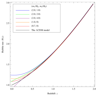
Figure 1: Redshift dependence of the Hubble rate function. The Hubble rate function is normalized by the Hubble constant of the $\Lambda$CDM model “$H_{0}$”. $\Omega_{\mathrm{m}}=0.31$, $\Omega_{\Lambda}=0.69$ is assumed in the $\Lambda$CDM model. While, $V_{1}$ is fixed by $V_{1}=1.8\kappa^{2}H_{0}^{2}$.

Matter density perturbation.

The master equation of the matter density contrast $\delta\equiv\delta\rho_{b}/\rho_{b}$ in mimetic matter model is given by Matsumoto:2015wja

$$\ddddot{\delta}+\left(7H-\frac{\dot{\lambda}}{\lambda}\right)\dddot{\delta}+\left(16H^{2}-4\kappa^{2}(\rho_{b}-2\lambda)-5H\frac{\dot{\lambda}}{\lambda}\right)\ddot{\delta}$$

$$+\frac{3}{2}\left(8H^{3}-3\kappa^{2}H(\rho_{b}-4\lambda)-4H^{2}\frac{\dot{\lambda}}{\lambda}+\kappa^{2}\rho_{b}\frac{\dot{\lambda}}{\lambda}\right)\dot{\delta}=0.$$ (13)

Equation (13) looks complicated, however, it shows that a quite similar behavior of the matter density contrast to that in the $\Lambda$CDM model. In the case of $V_{\phi}=0$, the master equation of the matter density contrast can be written as Matsumoto:2015wja

$$\ddot{\delta}_{\mathrm{tot}}+2H\dot{\delta}_{\mathrm{tot}}-\frac{\kappa^{2}}{2}\rho_{\mathrm{tot}}\delta_{\mathrm{tot}}=0,$$ (14)

where $\rho_{\mathrm{tot}}\equiv\rho_{b}-2\lambda$, $\delta_{\mathrm{tot}}\equiv(\delta\rho_{b}-2\delta\lambda)/(\rho_{b}-2\lambda)$. If we regard $\rho_{\mathrm{tot}}$ as $\rho_{\mathrm{m}}=\rho_{b}+\rho_{\mathrm{DM}}$, Eq. (14) is completely equivalent with the equation of the matter density contrast in the $\Lambda$CDM model. Paying attention to the fact that $V_{,\phi}\simeq 0$ is held around $z=10$ enables us to use $f(z=10)\simeq 1$, where $f\equiv d\ln\delta/dN$ is the growth factor of the matter density contrast and $N=\ln a$, as an initial condition of the numerical calculations. The calculation results of the growth factor are shown in Fig. 2. The deviations from the $\Lambda$CDM model in Fig. 2 appear in higher redshift and they become larger compared to those in Fig. 1. While, we can recognize that the lower growth rate is realized when the Hubble rate is higher as expected.

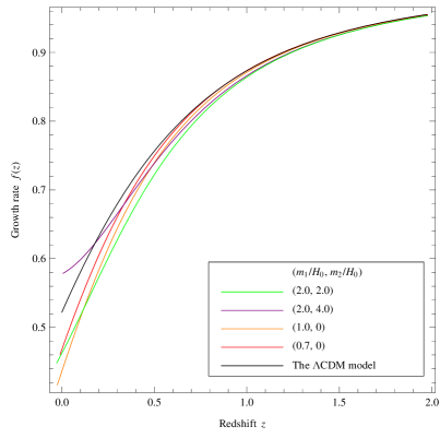
Figure 2: Evolution of the growth rate function $f(z)=d\ln\delta/dN$. The initial conditions are assigned as $f^{\prime\prime}(10)=f^{\prime}(10)=0$, and $f(10)=1$. The values of the parameters are same as those in Fig. 1.

Spherically symmetric solutions.

In the static space-time with spherical symmetry, $ds^{2}=-\mathrm{e}^{2\Phi(r)}dt^{2}+\mathrm{e}^{2\Psi(r)}dr^{2}+r^{2}(d\theta^{2}+\sin^{2}\theta d\varphi^{2})$, the constraint equation (6) is written by

$$\mathrm{e}^{-2\Psi}\phi^{\prime 2}+1=0.$$ (15)

Then, the Einstein equations in the case $\rho=p=0$ are given as

$$\frac{1}{\kappa^{2}}\left(\frac{1}{r^{2}}-\frac{2\Psi^{\prime}}{r}\right)\mathrm{e}^{-2\Psi}-\frac{1}{\kappa^{2}r^{2}}=-V,$$ (16)

$$\frac{1}{\kappa^{2}}\left(\frac{1}{r^{2}}+\frac{2\Phi^{\prime}}{r}\right)\mathrm{e}^{-2\Psi}-\frac{1}{\kappa^{2}r^{2}}=-V+2\lambda,$$ (17)

$$\frac{1}{\kappa^{2}}\left(\Phi^{\prime\prime}+\Phi^{\prime 2}-\Psi^{\prime}\Phi^{\prime}+\frac{\Phi^{\prime}}{r}-\frac{\Psi^{\prime}}{r}\right)\mathrm{e}^{-2\Psi}=-V.$$ (18)

The equation of the scalar field (5) yields

$$\lambda^{\prime}+\left(\Phi^{\prime}+\frac{2}{r}\right)\lambda-\frac{1}{2}\phi^{\prime}V_{,\phi}=0.$$ (19)

If $V_{\phi}=0$, it is possible to analyze the above equations, because Eq. (19) can be exactly solved Deruelle:2014zza ; Myrzakulov:2015sea . It is, in general, difficult to solve Eqs. (16)-(19), because of the nonlinearity of the equations. However, if we assume the conditions $|\Psi|,|r\Psi^{\prime}|,|\Phi|,|r\Phi^{\prime}|\ll 1$, we can evaluate the behavior of the functions $\Psi(r)$ and $\Phi(r)$ as follows. First, Eq. (15) gives

$$\phi(r)=\pm ir+const.$$ (20)

If we fix $const.=0$ in Eq. (20), the field $\phi(r)$ becomes pure imaginary. One may think it is problematic. However, there is no problem as long as the potential $V(\phi)$ is an even function, because the equations are, then, only described by the real functions. The concrete form of $\lambda(r)$ is given by solving Eq. (19) in the limit $|r\Phi^{\prime}|\ll 1$:

$$\lambda^{\prime}+\frac{2}{r}\lambda-\frac{1}{2}\phi^{\prime}V_{,\phi}=0.$$ (21)

While, if we express $\Phi(r)$ and $\Psi(r)$ as $\Phi(r)=r_{0}/r+\delta\Phi(r)$, where $r_{0}$ is a constant, and $\Psi(r)=-\Phi(r)+\delta\Psi(r)$, then Eqs. (16) and (17) yield

$$\delta\Psi^{\prime}(r)=\kappa^{2}r\lambda(r),$$ (22)

$$\partial_{r}(r\delta\Phi(r))=\delta\Psi(r)-\frac{\kappa^{2}r^{2}}{2}V(r)+\kappa^{2}r^{2}\lambda(r).$$ (23)

Here, $\delta\Phi(r)$ and $\delta\Psi(r)$ express the deviations from the vacuum solution $\Phi(r)=-\Psi(r)=r_{0}/r$. Equations (22) and (23) give the explicit forms of $\Phi(r)$ and $\Psi(r)$, however, we should remember that we first assume the conditions $|\Psi|,|r\Psi^{\prime}|,|\Phi|,|r\Phi^{\prime}|\ll 1$. By taking into account that $|r_{0}/r|=GM/r\ll 1$ is usually satisfied (e.g. $GM_{\odot}/R_{\odot}\sim 10^{-6}$), what we should make sure is the conditions $|\delta\Psi|,|r\delta\Psi^{\prime}|,|\delta\Phi|,|r\delta\Phi^{\prime}|\ll 1$. Substitutions of Eqs. (22) and (23) into $|\delta\Psi|,|r\delta\Psi^{\prime}|,|\delta\Phi|,|r\delta\Phi^{\prime}|\ll 1$, in general, give a constraint for $r$. In other words, the conditions $|\delta\Psi|,|r\delta\Psi^{\prime}|,|\delta\Phi|,|r\delta\Phi^{\prime}|\ll 1$ give a domain of the solutions (22) and (23). Then, the numerical calculations can be executed by regarding the solutions (22) and (23) as the boundary conditions, and the behavior of the solutions in the whole region will be clarified.

Let us consider the case that potential function is given by Eq. (3). In the region that $m_{1}r\sim m_{2}r\ll 1$, and $m_{3}r\ll 1$ are satisfied, the potential function $V(\phi)$ and its derivative are approximately expressed as $V(r)\sim V_{1}(1-m_{1}^{2}r^{2})+V_{2}(1-m_{3}^{4}r^{4})$, and $\phi^{\prime}V_{,\phi}(r)\sim-2(V_{1}m_{1}^{2}+2V_{2}m_{3}^{4}r^{2})r$. Then, Eq. (21) gives

$$\lambda(r)=\frac{s_{1}}{r^{2}}-\frac{1}{4}V_{1}m_{1}^{2}r^{2}-\frac{1}{3}V_{2}m_{3}^{4}r^{4},$$ (24)

where $s_{1}$ is an arbitrary constant. Substituting Eq. (24) into Eqs. (22) and (23) yields

$$\delta\Psi(r)=c_{1}+\kappa^{2}s_{1}\ln\frac{r}{r_{1}}-\frac{1}{16}\kappa^{2}V_{1}m_{1}^{2}r^{4}$$

$$-\frac{1}{18}\kappa^{2}V_{2}m_{3}^{4}r^{6},$$ (25)

$$\delta\Phi(r)=\frac{r_{2}}{r}+c_{1}+\kappa^{2}s_{1}\ln\frac{r}{r_{1}}-\frac{\kappa^{2}}{6}(V_{1}+V_{2})r^{2}$$

$$+\frac{3}{80}\kappa^{2}V_{1}m_{1}^{2}r^{4}+\frac{1}{63}\kappa^{2}V_{2}m_{3}^{4}r^{6},$$ (26)

where $r_{1}$, $r_{2}$, and $c_{1}$ are arbitrary constants. When the arbitrary constants $s_{1}$, $r_{2}$, and $c_{1}$ are negligibly small, $|\delta\Psi|\ll|\delta\Phi|\sim\kappa^{2}|V_{1}+V_{2}|r^{2}/6$ are held. Then, the condition $|\delta\Phi|\ll 1$ gives a constraint for $r$: $r\ll 10^{-2}H_{0}^{-1}$. Here, $V_{1}\sim H_{0}^{2}/\kappa^{2}$ and $V_{2}\sim 10^{5}H_{0}^{2}/\kappa^{2}$ are assumed. On the other hand, the conditions $m_{1}r\sim m_{2}r\ll 1$ and $m_{3}r\ll 1$ give $r\ll 10^{-5}H_{0}^{-1}$ if $m_{1}\sim m_{2}\sim H_{0}$, $m_{3}\sim 10^{5}H_{0}$. Therefore, Eqs. (24)-(26) are valid in the region $r\ll 10^{-5}H_{0}^{-1}$.

The behavior of the solutions around $r=10^{-5}H_{0}^{-1}$ are also comprehended by using Eqs. (24)-(26) as boundary conditions. The radius dependence of $\sqrt{r\delta\Phi^{\prime}(r)}$ in the region $r=10^{-6}H_{0}^{-1}-10^{-5}H_{0}^{-1}$ is shown in Fig. 3. $\delta\Phi(r)$ is well approximated as $\delta\Phi(r)\simeq-\kappa^{2}V_{2}r^{2}/6$ around $r=10^{-6}H_{0}^{-1}$, while, the damping factor $\mathrm{e}^{-m_{3}^{4}\phi^{4}}$ in Eq. (3) becomes effective when $r$ is larger than $10^{-6}H_{0}^{-1}$, therefore, the inclination of $\sqrt{r\delta\Phi^{\prime}(r)}$ becomes gentler than a straight line as seen in Fig. 3. The reason why $\sqrt{r\delta\Phi^{\prime}(r)}$ is plotted is that the rotation speed of a galaxy is approximately given by $v=\sqrt{r\Phi^{\prime}(r)}=\sqrt{r\Phi_{0}^{\prime}(r)+r\delta\Phi^{\prime}(r)}$, where $\Phi_{0}(r)$ is the Newtonian potential of the galaxy, if the circular motion is assumed. Namely, $\sqrt{r\delta\Phi^{\prime}(r)}$ represents the corrections for the rotation speed from mimetic matter. The curves in Fig. 3 may look rather steep, however, the potential made by baryons in the galaxy: $r\Phi_{0}^{\prime}(r)$ will make the rotation curve flatter.

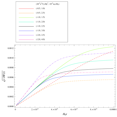
Figure 3: Contributions to the rotational velocity from mimetic matter. Here, the scale $10^{-6}cH_{0}^{-1}$ corresponds to $\sim 4$ kpc, and $v\simeq 3\sqrt{r\delta\Phi^{\prime}(r)}\times 10^{5}$ km s^-1 is given when $\Phi^{\prime}(r)\simeq\delta\Phi^{\prime}(r)$. The arbitrary constants in Eqs. (24)-(26) are fixed as $s_{1}$, $r_{2}$, $c_{1}=0$.

The gravitational behavior of our model in the solar system is given by

$$\delta\Psi(r)=c_{1}+\kappa^{2}s_{1}\ln\frac{r}{r_{1}},$$ (27)

$$\delta\Phi(r)=\frac{r_{2}}{r}+c_{1}+\kappa^{2}s_{1}\ln\frac{r}{r_{1}}-\frac{\kappa^{2}}{6}(V_{1}+V_{2})r^{2},$$ (28)

because the radius $r$ is enough small. If the arbitrary constants are fixed as $c_{1}=s_{1}=r_{2}=0$, then the solutions (27) and (28) are consistent with the Schwarzschild-de Sitter solution. We should note that $V_{2}$ is greater than usual cosmological constant by five orders of magnitude. However, it is known that the metric functions in Schwarzschild-de Sitter space-time can pass the solar system tests even if the value of the cosmological constant is greater than usual one by five orders of magnitude Kagramanova:2006ax .

Conclusions.

In this Letter, an example of the unified discription of dark energy and dark matter in mimetic matter model has been shown. This model can also describe the same time evolution of the Universe and the matter density perturbation as those in the $\Lambda$CDM model, however, the case that the Hubble rate function is greater than that of the $\Lambda$CDM model in low-redshift region have been, in particular, considered, because the recent observations of supernovae show such a behavior in the Hubble rate function. Then, the growth rate function of the matter density perturbation becomes less than that of the $\Lambda$CDM model. It is also consistent with the observational results. Whereas, the term $V_{2}\mathrm{e}^{-m_{3}^{4}\phi^{4}}$ has been introduced to explain the flat rotation curves of the spiral galaxies. This term does not influence the background evolution of the Universe, but influence the galaxy-scale physics. Moreover, it can easily pass the solar system tests of gravity. While, the corrections for gravity in the galaxy scale are independent from the mass of the galaxies. They only depend on the parameters $V_{2}$ and $m_{3}$. Therefore, detailed studies of the baryon density distribution of the galaxies will clarify whether or not this model is valid.

Appendix.

The work was supported by the Russian Government Program of Competitive Growth of Kazan Federal University.

References

- (1) A. G. Riess et al. [Supernova Search Team Collaboration], Astron. J. 116, 1009 (1998) [astro-ph/9805201].
- (2) S. Perlmutter et al. [Supernova Cosmology Project Collaboration], Astrophys. J. 517, 565 (1999) [astro-ph/9812133].
- (3) E. Komatsu et al. [WMAP Collaboration], Astrophys. J. Suppl. 192, 18 (2011) [arXiv:1001.4538 [astro-ph.CO]].
- (4) P. A. R. Ade et al. [Planck Collaboration], Astron. Astrophys. 571, A16 (2014) [arXiv:1303.5076 [astro-ph.CO]].
- (5) P. A. R. Ade et al. [Planck Collaboration], arXiv:1502.01589 [astro-ph.CO].
- (6) W. J. Percival et al. [SDSS Collaboration], Mon. Not. Roy. Astron. Soc. 401, 2148 (2010) [arXiv:0907.1660 [astro-ph.CO]].
- (7) C. Blake et al., Mon. Not. Roy. Astron. Soc. 418, 1707 (2011) [arXiv:1108.2635 [astro-ph.CO]].
- (8) F. Beutler et al., Mon. Not. Roy. Astron. Soc. 416, 3017 (2011) [arXiv:1106.3366 [astro-ph.CO]].
- (9) A. J. Cuesta et al., Mon. Not. Roy. Astron. Soc. 457, no. 2, 1770 (2016) [arXiv:1509.06371 [astro-ph.CO]].
- (10) T. Delubac et al. [BOSS Collaboration], Astron. Astrophys. 574, A59 (2015) [arXiv:1404.1801 [astro-ph.CO]].
- (11) A. H. Chamseddine and V. Mukhanov, JHEP 1311, 135 (2013) [arXiv:1308.5410 [astro-ph.CO]].
- (12) A. H. Chamseddine, V. Mukhanov and A. Vikman, JCAP 1406, 017 (2014) [arXiv:1403.3961 [astro-ph.CO]].
- (13) E. A. Lim, I. Sawicki and A. Vikman, JCAP 1005, 012 (2010) [arXiv:1003.5751 [astro-ph.CO]].
- (14) A. Golovnev, Phys. Lett. B 728, 39 (2014) [arXiv:1310.2790 [gr-qc]].
- (15) A. O. Barvinsky, JCAP 1401, no. 01, 014 (2014) [arXiv:1311.3111 [hep-th]].
- (16) A. G. Riess et al., Astrophys. J. 826, no. 1, 56 (2016) [arXiv:1604.01424 [astro-ph.CO]].
- (17) A. G. Riess et al., Astrophys. J. 730, 119 (2011) Erratum: [Astrophys. J. 732, 129 (2011)] [arXiv:1103.2976 [astro-ph.CO]].
- (18) E. Di Valentino, A. Melchiorri and J. Silk, Phys. Lett. B 761, 242 (2016) [arXiv:1606.00634 [astro-ph.CO]].
- (19) V. Marra, L. Amendola, I. Sawicki and W. Valkenburg, Phys. Rev. Lett. 110, no. 24, 241305 (2013) [arXiv:1303.3121 [astro-ph.CO]].
- (20) J. Matsumoto, S. D. Odintsov and S. V. Sushkov, Phys. Rev. D 91, no. 6, 064062 (2015) [arXiv:1501.02149 [gr-qc]].
- (21) N. Deruelle and J. Rua, JCAP 1409, 002 (2014) [arXiv:1407.0825 [gr-qc]].
- (22) R. Myrzakulov and L. Sebastiani, Gen. Rel. Grav. 47, no. 8, 89 (2015) [arXiv:1503.04293 [gr-qc]].
- (23) V. Kagramanova, J. Kunz and C. Lammerzahl, Phys. Lett. B 634, 465 (2006) [gr-qc/0602002].