A microscopic two–band model for the electron-hole asymmetry in high-$T_{c}$ superconductors and reentering behavior

Abstract

To our knowledge there is no rigorously analyzed microscopic model explaining the electron–hole asymmetry of the critical temperature seen in high–$T_{c}$ cuprate superconductors – at least no model not breaking artificially this symmetry. We present here a microscopic two–band model based on the structure of energetic levels of holes in $\mathrm{CuO}_{2}$ conducting layers of cuprates. In particular, our Hamiltonian does not contain ad hoc terms implying – explicitly – different masses for electrons and holes. We prove that two energetically near–lying interacting bands can explain the electron–hole asymmetry. Indeed, we rigorously analyze the phase diagram of the model and show that the critical temperatures for fermion densities below half–filling can manifest a very different behavior as compared to the case of densities above half–filling. This fact results from the inter–band interaction and intra–band Coulomb repulsion in interplay with thermal fluctuations between two energetic levels. So, if the energy difference between bands is too big (as compared to the energy scale defined by the critical temperatures of superconductivity) then the asymmetry disappears. Moreover, the critical temperature turns out to be a non–monotonic function of the fermion density and the phase diagram of our model shows “superconducting domes” as in high–$T_{c}$ cuprate superconductors. This explains why the maximal critical temperature is attained at donor densities away from the maximal one. Outside the superconducting phase and for fermion densities near half–filling the thermodynamics governed by our Hamiltonian corresponds, as in real high–$T_{c}$ materials, to a Mott–insulating phase. The nature of the inter–band interaction can be electrostatic (screened Coulomb interaction), magnetic (for instance some Heisenberg–type one–site spin–spin interaction), or a mixture of both. If the inter–band interaction is predominately magnetic then – additionally to the electron–hole asymmetry – we observe a reentering behavior meaning that the superconducting phase can only occur in a finite interval of temperatures. This phenomenon is rather rare, but has also been observed in the so–called magnetic superconductors. The mathematical results here are direct consequences of [J.-B. Bru, W. de Siqueira Pedra, Rev. Math. Phys. 22, 233–303 (2010)] which is reviewed in the introduction.

I Introduction

Theoretical foundations of superconductivity go back to the celebrated BCS theory – appeared in the late fifties (1957) – which explains conventional type I superconductors. The lattice version of this theory is based on the so–called (reduced) BCS Hamiltonian

$$\mathrm{H}_{\Lambda}^{BCS} : =\sum\limits_{k\in\Lambda_{N}^{\ast}}\left(\varepsilon_{k}-\mu\right)\left(\tilde{a}_{k,\uparrow}^{\ast}\tilde{a}_{k,\uparrow}+\tilde{a}_{k,\downarrow}^{\ast}\tilde{a}_{k,\downarrow}\right)$$ (1)

$$-\frac{1}{N}\sum_{k,q\in\Lambda_{N}^{\ast}}\gamma_{k,q}\tilde{a}_{k,\uparrow}^{\ast}\tilde{a}_{-k,\downarrow}^{\ast}\tilde{a}_{q,\downarrow}\tilde{a}_{-q,\uparrow}$$

defined in a cubic box $\Lambda_{N}:=\{\mathbb{Z}\cap[-L,L]\}^{3}$ of volume $|\Lambda_{N}|=N\geq 2$. We choose without loss of generality $N$ such that $L:=(N^{1/3}-1)/2\in\mathbb{N}$. Here $\Lambda_{N}^{\ast}$ is the reciprocal lattice of quasi–momenta (periodic boundary conditions) and the operator $\tilde{a}_{k,\mathrm{s}}^{\ast}$ (resp. $\tilde{a}_{k,\mathrm{s}}$) creates (resp. annihilates) a fermion with spin $\mathrm{s}\in\{\uparrow,\downarrow\}$ and (quasi–) momentum $k\in\Lambda_{N}^{\ast}$. The function $\varepsilon_{k}$ represents the kinetic energy and the real number $\mu$ is the chemical potential.

The BCS interaction is defined via the BCS coupling function $\gamma_{k,q}$ which is usually assumed in the physics literature to be – in momentum space – of the following form:

$$\gamma_{k,q}=\left\{\begin{array}[]{l}\gamma\geq 0\\ 0\end{array}\begin{array}[]{l}\mathrm{for\ }\left\|k-q\right\|\leq\mathrm{C}\\ \mathrm{for\ }\left\|k-q\right\|>\mathrm{C}\end{array}\right.$$ (2)

with $\mathrm{C}\in\left(0,\infty\right]$. The function $\gamma_{k,q}$ is not continuous in momentum space and so, it is slowly decaying, i.e., long range, in position space. (This means that it is not absolutely summable.) The case $\varepsilon_{k}=0$ is known as the strong coupling limit of the BCS model. Together with the choice $\mathrm{C}=\infty$, this case is of interest, as its analysis is easier and at the same time it qualitatively displays most of basic properties of real conventional type I superconductors, see, e.g., Chapter VII, Section 4 in Thou .

A general theory of superconductivity is, however, a subject of debate, especially for high–$T_{c}$ superconductors. An important phenomenon not taken into account in the BCS theory is the Coulomb interaction between electrons or holes, which can imply strong correlations – for instance in high–$T_{c}$ superconductors. This problem was of course already addressed in theoretical physics right after the emergence of the Fröhlich model and the BCS theory, see, e.g., Bogoliubov-tolman shirkov . Most of theoretical methods are based on perturbation theory or on the (non–rigorous) diagrammatic approach of Quantum Field Theory. However, even if these approaches have been successful in explaining many physical properties of superconductors Superconductivity2 ; Superconductivity3 only a few mathematically rigorous results related to a microscopic description of the quantum many–body problem exist as far as this problem is concerned, see for instance BruPedra1 .

Indeed, the results of BruPedra1 are based on an exact thermodynamic study of the phase diagram of the strong coupling BCS–Hubbard model defined in a cubic box $\Lambda_{N}:=\{\mathbb{Z}\cap[-L,L]\}^{D}$ of volume $|\Lambda_{N}|=N\geq 2$ by the Hamiltonian

$$\mathrm{H}_{N} : =-\mu\sum\limits_{x\in\Lambda_{N}}\left(n_{x,\uparrow}+n_{x,\downarrow}\right)-h\sum_{x\in\Lambda_{N}}\left(n_{x,\uparrow}-n_{x,\downarrow}\right)$$

$$+2\lambda\sum_{x\in\Lambda_{N}}n_{x,\uparrow}n_{x,\downarrow}-\frac{\gamma}{N}\sum_{x,y\in\Lambda_{N}}a_{x,\uparrow}^{\ast}a_{x,\downarrow}^{\ast}a_{y,\downarrow}a_{y,\uparrow}$$

for real parameters $\mu,h\in\mathbb{R}$ and $\lambda,\gamma\geq 0$. The operator $a_{x,\mathrm{s}}^{\ast}$ (resp. $a_{x,\mathrm{s}}$) creates (resp. annihilates) a fermion with spin $\mathrm{s}\in\{\uparrow,\downarrow\}$ at lattice position $x\in\mathbb{Z}^{D}$, $D=1,2,3,...,$ whereas $n_{x,\mathrm{s}}:=a_{x,\mathrm{s}}^{\ast}a_{x,\mathrm{s}}$ is the particle number operator at position $x$ and spin $\mathrm{s}$. The first term of the right hand side of (LABEL:Hamiltonian_BCS-Hubbard) represents the strong coupling limit of the kinetic energy, also called “atomic limit” in the context of the Hubbard model, see, e.g., atomiclimit1 ; atomiclimit2 . The second term corresponds to the interaction between spins and the magnetic field $h$. The one–site interaction with positive coupling constant $\lambda\geq 0$ represents the (screened) Coulomb repulsion as in the celebrated Hubbard model. The last term is the BCS interaction written in the $x$–space since

$$\frac{\gamma}{N}\sum_{x,y\in\Lambda_{N}}a_{x,\uparrow}^{\ast}a_{x,\downarrow}^{\ast}a_{y,\downarrow}a_{y,\uparrow}=\frac{\gamma}{N}\sum_{k,q\in\Lambda_{N}^{\ast}}\tilde{a}_{k,\uparrow}^{\ast}\tilde{a}_{-k,\downarrow}^{\ast}\tilde{a}_{q,\downarrow}\tilde{a}_{-q,\uparrow},$$ (4)

see (2) with $\mathrm{C}=\infty$. This homogeneous BCS interaction should be seen as a long range effective interaction for which the corresponding mediator does not matter, i.e., it could be due to phonons, as in conventional type I superconductors, or anything else. From theoretical considerations remark that phonons can probably not be responsible of superconductivity above 90K, see, e.g., Emery .

The Hamiltonian (LABEL:Hamiltonian_BCS-Hubbard) defines in the thermodynamic limit $N\rightarrow\infty$ a free energy density functional on a suitable set of states of the fermionic observable algebra of the lattice $\mathbb{Z}^{D}$ ($D$–dimensional crystal). See (BruPedra1, , Section 6.2) for details. Minimizers $\omega$ of the free energy density are called equilibrium states of the model. We say that the model has a superconducting phase – at fixed parameters – if there is at least one equilibrium state $\omega$ of the model for which $\omega(a_{x,\downarrow}a_{x,\uparrow})\neq 0$, i.e., if the $U(1)$–gauge symmetry is spontaneously broken.

The main properties of the phase diagram of the strong coupling BCS–Hubbard model described in BruPedra1 can be summarized as follows:

• There is a non–empty set of parameters $\mathcal{S}$ defining a s–wave superconducting phase with off–diagonal long range order.

• Depending on parameters the superconducting phase transition is either of first order or of second order (see Fig. 1).

• The superconducting phase $\mathcal{S}$ is characterized by the formation of Cooper pairs and a depleted Cooper pair condensate, the density $\mathit{r}_{\beta}\in[0,1/4]$ of which is defined by the gap equation.

• There is a Meißner effect concerning the relationship between superconductivity and magnetization. The Meißner effect is defined here by the absence of magnetization in presence of superconductivity. Steady surface currents around the bulk of the superconductor are not analyzed as it is a finite volume effect.

• There exists a superconductor–Mott insulator phase transition for near–one fermion densities per lattice site (see Fig. 2).

• The coexistence of ferromagnetic and superconducting phases is shown to be feasible at (critical) points of the boundary $\partial\mathcal{S}$ of $\mathcal{S}$.

• The critical temperature $\theta_{c}$ can be (locally) an increasing function of the positive coupling constant $\lambda\geq 0$ at fixed chemical potential $\mu\in\mathbb{R}$ (see Fig. 1), but not at fixed fermion density $\rho>0$.

• For $\lambda\sim\gamma$ the critical temperature $\theta_{c}$ shows – as a function of the fermion density $\rho$ – the typical “superconducting domes” observed in high–$T_{c}$ superconductors: $\theta_{c}$ is zero or very small for $\rho\sim 1$ and is much larger for $\rho$ away from $1$ (see Fig. 2). The latter gives a rigorous explanation of the need of doping Mott insulators to obtain superconductors.

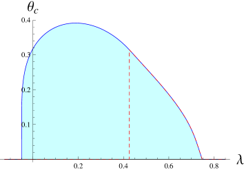
Figure 1: Illustration of the critical temperature $\theta_{c}$ for $\gamma=2.6,$ $h=0$, $\mu=1.25$, and $\lambda\in[-0.1,0.85]$. The blue line corresponds to a second order phase transition, whereas the red dashed line represents the domain of $\lambda$ with a first order phase transition.

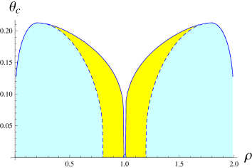
Figure 2: Illustration of the critical temperature $\theta_{c}$ for $\gamma=2.6,$ $h=0.1$, $\lambda=0.575$, and fermion densities $\rho\in[0,2]$. The blue and yellow region correspond respectively to the superconducting and ferromagnetic–superconducting phases.

This model is of course too simplified with respect to (w.r.t.) real superconductors. For instance, the anti–ferromagnetic phase or the presence of vortices, which can appear in (type II) high–$T_{c}$ superconductors, are not observed. However, since the range of parameters in which we are interested turns out to be related to a first order phase transition, by high–low temperature expansions the – more realistic – model including kinetic terms

$$\mathrm{H}_{N,\varepsilon}:=\mathrm{H}_{N}+\sum\limits_{x,y\in\Lambda_{N}}\varepsilon(x-y)\left(a_{y,\downarrow}^{\ast}a_{x,\downarrow}+a_{y,\uparrow}^{\ast}a_{x,\uparrow}\right)$$ (5)

should have essentially the same correlation functions as $\mathrm{H}_{N}$ – up to corrections of order $||\varepsilon||_{1}$ ($\ell^{1}$–norm of $\varepsilon$). Thus, the Hamiltonian $\mathrm{H}_{N}$ may be a good model for certain kinds of superconductors or ultra–cold Fermi gases in optical lattices for which the strong coupling regime is justified, especially because all parameters of $\mathrm{H}_{N}$ have a phenomenological interpretation and can be directly related to experiments, see (BruPedra1, , Sect. 5).

Since the discovery of mercury superconductivity in 1911 a significant amount of superconducting materials has been found. This includes usual metals, like lead, aluminum, zinc or platinum, magnetic materials, heavy–fermion systems, organic compounds and ceramics. High–$T_{c}$ cuprate superconductors are among the most interesting superconducting materials for applications. In spite of that, a general microscopic theory explaining conveniently their thermodynamics is still not available. For instance, the experimentally well–known electron–hole asymmetry of high–$T_{c}$ superconductors which usually show higher critical temperatures for donors of holes than for donors of electrons, is not clearly understood from the microscopic point of view. As far as we know no microscopic theory can give up to now some incontestable explanation of this fact unless one artificially breaks the electron–hole symmetry of models (for instance by imposing explicitly two different mass for electrons and holes). In fact, the most plausible explanation of the electron–hole asymmetry is given in Superconductivity2 ; Superconductivity3 and is also based on two–band (Hubbard or $t-J$) models in the strong coupling regime. These studies are debatable and we discuss them in relation with our approach in Section II after introducing our two–band model.

The usual BCS model and the strong coupling BCS–Hubbard model have structural properties preventing their critical temperatures of superconductivity from being asymmetric w.r.t. the density of donors. The strong coupling BCS–Hubbard shows – at least and in contrast to the usual BCS model – the typical (though symmetric) “superconducting domes” of high–$T_{c}$ materials for the critical temperature. Therefore, the first objective is to investigate generalizations of the strong coupling BCS–Hubbard in order to find plausible – microscopic – explanations for the electron–hole asymmetry in high–$T_{c}$ cuprate superconductors. The (one–band) strong coupling BCS–Hubbard is a good starting point for further investigations on high–$T_{c}$ phenomenology, also because it correctly describes the non–superconducting phase of cuprates near half–filling, which is Mott–insulating and not metallic as in usual superconductors.

Another class of superconductors which would be interesting to study are ferromagnetic superconductors (Shrivastava, , p. 263-267). Indeed, these materials exhibit some peculiar features not found in ordinary superconductors, one of these being the reentering behavior: The system becomes superconducting below a critical temperature $\theta_{c_{1}}$ and then magnetically ordered but not superconducting below $\theta_{c_{2}}$ with $\theta_{c_{2}}<\theta_{c_{1}}$. Additionally, coexistence of a ferromagnetic phase and superconductivity seems also to appear around $\theta_{c_{2}}$, at least for some ferromagnetic superconductors. Motivated by the thermodynamic behavior of ferromagnetic superconductors, the second goal of this paper is to show that a magnetic inter–band interaction can be responsible for a reentering behavior.

We introduce a two–band model by using two copies of the (one–band) model $\mathrm{H}_{N}$ defined by (LABEL:Hamiltonian_BCS-Hubbard) and by adding an inter–band interaction term. The parameters of the first band, called here the “$\mathit{s}$”–band, are chosen such that a superconducting phase appears at low enough temperatures if no interaction with the second band is present. By contrast, the parameters of the second band, called the “$\mathit{f}$”–band, are such that without interaction with the “$\mathit{s}$”–band one would have a (generally ferromagnetic) Mott–insulating phase at low temperatures.

We prove that the thermodynamic behavior of such a two–band model inherits of course properties of the thermodynamic behavior of the one–band model $\mathrm{H}_{N}$ described in BruPedra1 , but also shows additional features:

• There is an electron–hole asymmetry w.r.t. the critical temperature of superconductivity which results from the inter–band interaction and intra–band Coulomb repulsion in interplay with thermal fluctuations between the “$\mathit{s}$”– and “$\mathit{f}$”–bands.

• Choosing the relative strength of parameters to each other according to experimental data about the energy levels of holes in $\mathrm{CuO}_{2}$ layers of high–$T_{c}$ cuprate superconductors, we show that this asymmetry is in favor of a doping with donors of holes. This is just what is seen in cuprates.

• There is a (rather small) set of parameters with a reentering behavior coming from a magnetic inter–band interaction.

• There is a kind of “microscopic Meißner effect”: The increase of the magnetic inter–band interaction destroys superconductivity without need of any magnetization induced by an external magnetic field. It follows that a reentering behavior can also appear without any ferromagnetism.

Our two–band model is certainly not the final microscopic theory of high–$T_{c}$ cuprate superconductors even if one includes a small kinetic part as explained above. However, we are convinced that the model and analysis presented here highlight microscopic processes playing a crucial role in which concerns the phenomenology of high–$T_{c}$ materials – or at least a relevant part of it.

The method presented in BruPedra1 and used here gives access to domains of the phase diagram usually difficult to reach via other standard mathematical tools. For instance, the existence of the superconductor–Mott insulator phase transition for near–one fermion densities per lattice site (see Fig. 2) can neither be obtained by perturbation theory nor by spin reflection positivity Lieb-reflexion arguments. Indeed, the spin reflection positivity described for instance in Tian cannot give access to such a phenomenon as it requires a fermion density exactly equal to one. Also, the regime in which the superconducting domes are observed corresponds to the choice $\lambda\sim\gamma$ and they are never seen if $\lambda$ is too small as compared to $\gamma$. Thus, perturbative arguments around the purely BCS case $\lambda=0$ are inadequate. The results given here may be rigorously obtained by renormalization group techniques, but this method of analysis would be – from the technical point of view – probably much more demanding than the approach of BruPedra1 .

As a final remark the one–band and two–band models discussed here should be seen as a kind of “solvable” class of models capturing important phenomenological aspects and from which one can implement physically more realistic models – for instance by using perturbation theory. Indeed, a first natural extension of the two–band model – beyond the introduction of a small kinetic term as explained above – is the addition of a Heisenberg–type interaction for fermions within the non–superconducting band in order to spontaneously create a ferromagnetic phase and to get a reasonable microscopic theory of ferromagnetic superconductors. Another possible generalization is the introduction of a small inter–band interaction term describing tunneling effects between bands (inter–band hopping), see below (10).

II The two–band model

In order to fix ideas about the microscopic structure of typical high–$T_{c}$ materials we consider the case of cuprates. It is known from experimental physics that superconducting carriers, mainly holes in the case of cuprates, move within two–dimensional $\mathrm{CuO}_{2}$ layers made of $\mathrm{Cu}^{++}$ and $\mathrm{O}^{--}$, see, e.g., (Saxena, , Fig. 5.3. p. 127).

$\mathrm{Cu}^{+}=(\mathrm{Ar})3d^{10}$ is a closed shell configuration (see, e.g., Emery or (Saxena, , Sect. 5.5)). Then the last occupied orbital of the copper cations $\mathrm{Cu}^{++}=(\mathrm{Ar})3d^{9}$ is almost full, i.e., it can be modelled by a half–filled band of holes (exactly one hole per lattice site). Putting a further hole in one copper cation, i.e., transforming $\mathrm{Cu}^{++}$ into $\mathrm{Cu}^{+++}$, costs some positive amount $2\lambda_{\mathrm{Cu}}>0$ of energy. The latter justifies the presence of a repulsion term of the form

$$2\lambda_{\mathrm{Cu}}n_{x,\uparrow}^{(\mathrm{Cu})}n_{x,\downarrow}^{(\mathrm{Cu})}\quad\mathrm{with\ }\lambda_{\mathrm{Cu}}>0$$

at each (two–dimensional) lattice site $x$ for the copper band.

$\mathrm{O}^{--}=(\mathrm{Be})2p^{6}$ corresponds to a closed shell configuration as well (see, e.g., Emery or (Saxena, , Sect. 5.5)) and therefore, the oxygen orbitals in the $\mathrm{CuO}_{2}$ layers of cuprates can be modelled by an empty band of holes provided there is no doping. Indeed, by doping cuprates holes can be added to orbitals of $\mathrm{O}^{--}$ in the $\mathrm{CuO}_{2}$ layers. Putting one new hole on an oxygen site analogously costs some positive amount $\delta_{\mathrm{Cu-O}}>0$ of energy relatively to the energy of the half–filled $\mathrm{Cu}^{++}$ orbital. This justifies the assumption that the difference between chemical potentials $\mu_{\mathrm{Cu}}$ and $\mu_{\mathrm{O}}$ of the copper and oxygen bands is some strictly positive quantity $\delta_{\mathrm{Cu-O}}>0$, i.e.,

$$\mu_{\mathrm{Cu}}=\mu_{\mathrm{O}}+\delta_{\mathrm{Cu-O}}>\mu_{\mathrm{O}}\ .$$ (6)

Experiments on cuprates indicate that $\lambda_{\mathrm{Cu}}\approx 4\rm{eV}$ and $\delta_{\mathrm{Cu-O}}\leq 2\rm{eV}$ (at least in (Saxena, , Fig. 5.9. p. 132)). So, $\delta_{\mathrm{Cu-O}}$ should be chosen small as compared to the intra–band repulsion $\lambda_{\mathrm{Cu}}$. At any site $x$ of the $\mathrm{CuO}_{2}$ lattice it is also natural to assume that two carriers experience an intra–band repulsion

$$2\lambda_{\mathrm{O}}n_{x,\uparrow}^{(\mathrm{O})}n_{x,\downarrow}^{(\mathrm{O})}\quad\mathrm{with\ }\lambda_{\mathrm{O}}\geq 0$$

when they are both on the oxygen  site and an inter–band repulsion

$$2\lambda_{\mathrm{Cu-O}}(n_{x,\uparrow}^{(\mathrm{O})}+n_{x,\downarrow}^{(\mathrm{O})})(n_{x,\uparrow}^{(\mathrm{Cu})}+n_{x,\downarrow}^{(\mathrm{Cu})})\quad\mathrm{with\ }\lambda_{\mathrm{Cu-O}}\geq 0$$

if one carrier is on the oxygen site and the other one on the copper site, see, e.g., (Emery, , Eq. (1)). More precise experimental data about the strength of the couplings $\lambda_{\mathrm{O}}$ and $\lambda_{\mathrm{Cu-O}}$ in real cuprates would be useful.

To each of these (almost independent) $\mathrm{CuO}_{2}$ conducting layers there is a second layer of another chemical nature which acts as a charge reservoir and provides conduction fermions to the $\mathrm{CuO}_{2}$ layer. These reservoir layers can be engineered in order to get the desired density of carriers (holes or electrons). In $\mathrm{La}_{2-x}\mathrm{Sr}_{x}\mathrm{CuO}_{4}$ compounds the holes added to $\mathrm{CuO}_{2}$ layers of $\mathrm{La}_{2}\mathrm{CuO}_{4}$ directly go into the oxygen band which is experimentally shown to be at the origin of superconductivity. Indeed, holes on copper bands cannot directly participate in superconductivity by forming Cooper pairs, see (Saxena, , p. 133). Additionally, the hopping amplitude of holes within $\mathrm{CuO}_{2}$ layers of $\mathrm{La}_{2-x}\mathrm{Sr}_{x}\mathrm{CuO}_{4}$ is smaller or equal than $1\rm{eV}\leq\delta_{\mathrm{Cu-O}}\leq 2\lambda_{\mathrm{Cu}}$. In particular, the assumption of strong coupling regime is far from being unrealistic in this case. For more details we recommend Saxena , in particular Chapter 5.

As suggested in (Saxena, , Sect. 5.12) we define a two–band model in relation to the physics described above. We use two lattices $\mathfrak{L}_{\mathit{s}}$ and $\mathfrak{L}_{\mathit{f}}$ corresponding respectively to a “$\mathit{s}$”–band of superconducting fermions and a “$\mathit{f}$”–band of ferromagnetic fermions (electrons, holes or even more general fermions, like fermionic magnetic atoms). In particular, the “$\mathit{s}$”–band is interpreted within $\mathrm{CuO}_{2}$ conducting layers in cuprates as the oxygen band, whereas the “$\mathit{f}$”–band corresponds to the copper band. To simplify our study, we assume that both lattices are of the same type: $\mathfrak{L}_{\mathit{s}}\sim\mathfrak{L}_{\mathit{f}}\sim\mathbb{Z}^{D}$, $D=1,2,3,...$ In this context the thermodynamics of the two–band system is governed by the (strong coupling) Hamiltonian

$$\mathrm{H}_{N}^{(\mathit{s},\mathit{f})}:=\mathrm{H}_{N}^{(\mathit{s})}\otimes\mathbf{1}+\mathbf{1}\otimes\mathrm{H}_{N}^{(\mathit{f})}+\mathrm{V}_{N}$$ (7)

where $N=|\Lambda_{N}|<\infty$ is the volume of the box $\Lambda_{N}:=\{\mathbb{Z}\cap[-L,L]\}^{D}$ seen as a subset of either $\mathfrak{L}_{\mathit{s}}$ or $\mathfrak{L}_{\mathit{f}}$. Here $\mathbf{1}$ is the identity on the fermion Fock space related to either $\mathfrak{L}_{\mathit{s}}$ or $\mathfrak{L}_{\mathit{f}}$. In this model the kinetic energy is neglected as the strong coupling regime is realistic for $\mathrm{CuO}_{2}$ layers. In fact, without changing qualitatively the phenomenology a small kinetic energy could be added as explained around (5). Accordingly, the self–adjoint operator

$$\mathrm{H}_{N}^{(\mathit{s})}:=\mathrm{H}_{N}\left(\mu_{\mathit{s}},h_{\mathit{s}},\lambda_{\mathit{s}},\gamma_{\mathit{s}}\right)$$

is the Hamiltonian of “$\mathit{s}$”–fermions defined from $\mathrm{H}_{N}$ with $\mu_{\mathit{s}},h_{\mathrm{s}}\in\mathbb{R}$ and $\lambda_{\mathit{s}},\gamma_{\mathit{s}}\geq 0$, whereas

$$\mathrm{H}_{N}^{(\mathit{f})}:=\mathrm{H}_{N}\left(\mu_{\mathit{f}},h_{\mathit{f}},\lambda_{\mathit{f}},0\right)$$

is the Hamiltonian of “$\mathit{f}$”–fermions with $\mu_{\mathit{f}},h_{\mathit{f}}\in\mathbb{R}$ and $\lambda_{\mathit{f}}\geq 0$. Similarly to the discussion above about the energy levels in copper and oxygen bands of $\mathrm{CuO}_{2}$ layers, we write

$$\mu_{\mathit{f}}:=\mu_{\mathit{s}}+\delta\quad\mathrm{with}\ \delta\in\mathbb{R}.$$ (8)

In particular, if $\delta>0$, then the “$\mathit{f}$”–band is energetically lower than the “$\mathit{s}$”–band, whereas $\delta<0$ means the opposite. As far as $\mathrm{CuO}_{2}$ layers are concerned the energy difference $\delta=\delta_{\mathrm{Cu-O}}>0$ must be positive and small w.r.t. the repulsive coupling constant $\lambda_{\mathit{f}}=\lambda_{\mathrm{Cu}}\geq 0$. The inter–band interaction equals

$$\mathrm{V}_{N} : =2\lambda\sum_{x\in\Lambda_{N}}(n_{x,\uparrow}^{(\mathit{s})}+n_{x,\downarrow}^{(\mathit{s})})(n_{x,\uparrow}^{(\mathit{f})}+n_{x,\downarrow}^{(\mathit{f})})$$ (9)

$$-\eta\sum_{x\in\Lambda_{N}}(n_{x,\uparrow}^{(\mathit{s})}-n_{x,\downarrow}^{(\mathit{s})})(n_{x,\uparrow}^{(\mathit{f})}-n_{x,\downarrow}^{(\mathrm{f})})$$

with $\lambda\geq 0$ and $\eta\in\mathbb{R}$. Here $n_{x,\mathrm{s}}^{(\mathit{s})}$ (resp. $n_{x,\mathrm{s}}^{(\mathit{f})}$) is the particle number operator of “$\mathit{s}$”– (resp. “$\mathit{f}$”–) fermions at position $x\in\mathbb{Z}^{D}$ and spin $\mathrm{s}\in\{\uparrow,\downarrow\}$. The first term of the inter–band interaction $\mathrm{V}_{N}$ represents the screened Coulomb interaction between “$\mathit{s}$”– and “$\mathit{f}$”–fermions, i.e., between carriers in the copper and oxygen bands of the $\mathrm{CuO}_{2}$ conducting layers. If $\eta\neq 0$ then the second term in $\mathrm{V}_{N}$ represents a magnetic interaction between “$\mathit{s}$”– and “$\mathit{f}$”–fermions on the same site of the lattices $\mathfrak{L}_{\mathit{s}}$ and $\mathfrak{L}_{\mathit{f}}$.

Note that the superconducting phase which appears for “$\mathit{s}$”–fermions in our two–band model, is a (perfect) s–wave phase (cf. (BruPedra1, , Thm 3.3)) for all $D=1,2,3,...$ The dimension $D=2$ of conducting layers is of course extremely important for the physics of high–$T_{c}$ cuprate superconductors. Moreover, experiments usually suggest that d–wave superconductivity can appear in cuprate high–$T_{c}$ superconductors and this is an important physical aspect of high–$T_{c}$ superconductors. The latter as well as the anti-ferromagnetism in cuprates are not studied here. However, as the phenomenology which emerges is coherent with experiments, the dimensionality of conducting layers, the anti-ferromagnetism, and the kind of pairing of superconducting carriers do not seem to be relevant for the phenomenon we are interested in, namely the influence of multi–band structures on the phase diagram of generic superconductors.

For instance, the phenomenon we present here highlight why the explanation given in Superconductivity2 ; Superconductivity3 of the electron-hole asymmetry works. This approach is, indeed, based on a two-band model in the strong coupling regime. However, in contrast to our approach, the two bands in Superconductivity2 ; Superconductivity3 come from two different hopping terms, representing respectively the nearest–neighbor and next–nearest–neighbor hopping. Their studies are far from being mathematically rigorous and can thus be debatable. Our paper is a mathematical proof that the kinetic energy is not necessary to explain this asymmetry and shows the importance of close multi-band structures (even in presence of small kinetic terms as explained around (5) and (7)). In fact, even if Superconductivity2 ; Superconductivity3 is physically correct, the explanations Superconductivity2 ; Superconductivity3 are not transparent (at least to the non–expert) and we think that our paper gives a much clearer understanding why that should work, where this asymmetry comes from, and how that can be used to draw different conclusions (cf. Section III, cases (a)–(d)).

Observe also that the bands are denoted by “$\mathit{s}$” for “superconducting” and by “$\mathit{f}$” for “ferromagnetic” or “fixed”. The charge carriers can be here fermions of any kind. In cuprates such fermions should be seen as holes (of electrons). Indeed, the two–band model can emerge from other physical systems or interpretations. For instance, the “$\mathit{s}$”–band could have represented holes within $\mathrm{CuO}_{2}$ layers, whereas “$\mathit{f}$”–fermions could have been seen as holes within the charge reservoir layer. Another example could have been given by considering some tunneling between the conducting layer and the charge reservoir layer. The tunneling modes could then give origin to different effective energy levels. The latter can be interpreted as a discrete component of the kinetic energy in the direction perpendicular to the conduction plane. Indeed, we can assume that the layers of high–$T_{c}$ materials can be decomposed in independent groups of finitely many layers (for instance groups of two layers in the case of cuprates: One $\mathrm{CuO}_{2}$ layer and one reservoir layer). Using periodic boundary conditions the kinetic energy w.r.t. the perpendicular direction to the conduction planes is – in this case – a discrete quantity and leads to the formation of finitely many different energetic levels per site. With this example the “$\mathit{s}$”–band  would have represented holes or electrons with a zero perpendicular kinetic energy, whereas the “$\mathit{f}$”–band would have corresponded to holes or electrons moving with a velocity having a non–vanishing component perpendicularly to the conduction planes.

Now, the first question we have to address in order to obtain the thermodynamics of the system is the computation of the grand–canonical pressure

$$\mathrm{p}:=\underset{N\rightarrow\infty}{\lim}\frac{1}{\beta N}\ln\mathrm{Trace}\left(e^{-\beta\mathrm{H}_{N}^{(\mathit{s},\mathit{f})}}\right)<\infty$$

in the thermodynamic limit $N\rightarrow\infty$ at fixed inverse temperature $\beta>0$. Such an analysis is performed rigorously in BruPedra1 for the one–band case (see also Section V) and can easily be extended to the two–band model $\mathrm{H}_{N}^{(\mathit{s},\mathit{f})}$. Using the methods of BruPedra1 (see Section V) together with explicit computations we get the following result:

Theorem 1

For any real $\mu_{\mathit{s}}$, $h_{\mathit{s}}$, $\mu_{\mathit{f}}$, $h_{\mathit{f}}$, $\eta$ and positive numbers $\gamma_{\mathit{s}}$, $\lambda_{\mathit{s}}$, $\lambda_{\mathit{f}}$, $\lambda$, $\beta>0$,

$$\mathrm{p}:=\beta^{-1}\ln 2+\mu_{\mathit{s}}+\mu_{\mathit{f}}+\sup_{r\geq 0}\left\{-\gamma_{\mathit{s}}r+\beta^{-1}\ln\mathrm{f}(r)\right\}$$

with

$$\mathrm{f}(r) = (\mathrm{e}^{-\beta\mu_{\mathit{f}}}+\mathrm{e}^{-\beta(4\lambda+2\lambda_{\mathit{f}}-\mu_{\mathit{f}})})\cosh(\beta h_{\mathit{s}})$$

$$+\mathrm{e}^{-\beta(2\lambda-h_{\mathit{s}})}\cosh(\beta(\eta+h_{\mathit{f}}))$$

$$+\mathrm{e}^{-\beta(2\lambda+h_{\mathit{s}})}\cosh(\beta(\eta-h_{\mathit{f}}))$$

$$+\mathrm{e}^{-\beta(\lambda_{\mathit{s}}+\mu_{\mathit{f}})}\cosh(\beta g_{r,0})$$

$$+\mathrm{e}^{-\beta(4\lambda+\lambda_{\mathit{s}}+2\lambda_{\mathit{f}}-\mu_{\mathit{f}})}\cosh(\beta g_{r,4\lambda})$$

$$+2\mathrm{e}^{-\beta(2\lambda+\lambda_{\mathit{s}})}\cosh(\beta h_{\mathit{f}})\cosh(\beta g_{r,2\lambda})$$

and $g_{r,x}:=\{(x+\lambda_{\mathit{s}}-\mu_{\mathit{s}})^{2}+\gamma_{\mathit{s}}^{2}r\}^{1/2}$.

The exact form of the function $\mathrm{f}$ is only given for completeness. What is important is that it is some explicitly given function in the thermodynamic limit – even if we do not know, a priori, how to diagonalize the Hamiltonian $\mathrm{H}_{N}^{(\mathit{s},\mathit{f})}$ at any fixed $N\in\mathbb{N}$. This fact is important as it makes possible a computer aided rigorous analysis of the thermodynamic problem. There is, however, a certain amount on luckiness about this: The function $\mathrm{f}$ is obtained from the eigenvalues of some $(16\times 16)$–matrix, the so–called approximating Hamiltonian of the model (see BruPedra1 and Section V for details), depending on the parameters of the model. By a well–known theorem of algebra there is no explicit general formula for the solutions of polynomial equations of degree greater than four. So, it is a rather surprising property of the characteristic polynomial (which has degree $16$) of the matrix corresponding to the approximating Hamiltonian of our problem to have explicitly known zeros for any choice of parameters.

In fact, it would have been natural to include in our model $\mathrm{H}_{N}^{(\mathit{s},\mathit{f})}$ a hopping term of the form

$$\sum\limits_{x\in\Lambda_{N},\mathrm{s}\in\{\uparrow,\downarrow\}}t_{\mathit{s},\mathit{f}}\left((a_{x,\mathrm{s}}^{(\mathit{s})})^{\ast}a_{x,\mathrm{s}}^{(\mathit{f})}+(a_{x,\mathrm{s}}^{(\mathit{f})})^{\ast}a_{x,\mathrm{s}}^{(\mathit{s})}\right)$$ (10)

which on all lattice sites $x\in\Lambda_{N}$ annihilates a fermion in “$\mathit{f}$”–band to create another one within the “$\mathit{s}$”–band and vice–versa. Theorem 1 would still be satisfied for any $t_{\mathit{s},\mathit{f}}\in\mathbb{R}$, but the function $\mathrm{f}$ would then be more difficult to obtain as the eigenvalues of the resulting $(16\times 16)$–matrix are not that easy to compute. However, the hopping term (10), which is important in the analysis dynamical properties, should have almost no effect on the thermodynamics of the system at equilibrium – at least if $|t_{\mathit{s},\mathit{f}}|$ is sufficiently small. This conjecture could anyway be verified – but with a significant numerical effort on the diagonalization of the corresponding $(16\times 16)$–matrix.

To conclude, let $\mathfrak{R}\subseteq[0,\infty)$ be the set of solutions $\mathit{r}_{\beta}\geq 0$ of the variational problem

$$\underset{r\geq 0}{\sup}\left\{-\gamma_{\mathit{s}}r+\beta^{-1}\ln\mathrm{f}(r)\right\}=-\gamma_{\mathit{s}}\mathit{r}_{\beta}+\beta^{-1}\ln\mathrm{f}(\mathit{r}_{\beta})$$ (11)

given by Theorem 1. Observe that $\mathfrak{R}\neq\varnothing$ is a non–empty compact set since $\mathrm{f}(r)=\mathcal{O}(\mathrm{e}^{\beta\gamma_{\mathit{s}}\sqrt{r}})$ when $r\rightarrow\infty$. Let

$$\mathfrak{E}:=\{z_{\beta}=\sqrt{\mathit{r}_{\beta}}e^{i\varphi}:\varphi\in[0,2\pi),\;\mathit{r}_{\beta}\in\mathfrak{R}\}\subset\mathbb{C}.$$

Exactly as in the case of the one–band model $\mathrm{H}_{N}$ (cf. (BruPedra1, , Section 6.2)) the set $\mathfrak{E}$ parameterizes (one–to–one) the pure equilibrium states of the model $\mathrm{H}_{N}^{(\mathit{s},\mathit{f})}$. The equilibrium state $\omega$ is called pure, if $\omega=\lambda\omega_{1}+(1-\lambda)\omega_{2}$ for equilibrium states $\omega_{1},\omega_{2}$ and some $\lambda\in(0,1)$ implies $\omega_{1}=\omega_{2}=\omega$. The parameterization $\mathfrak{E}\ni z_{\beta}\mapsto\omega_{z_{\beta}}$ can be chosen to be continuous and such that $\omega_{z_{\beta}}(a_{x,\downarrow}^{(\mathit{s})}a_{x,\uparrow}^{(\mathit{s})})=z_{\beta}$ for all $x\in\mathbb{Z}^{D}$. In particular, if $\mathit{r}_{\beta}\in$ $\mathfrak{R}$, $\mathit{r}_{\beta}>0$, then the model $\mathrm{H}_{N}^{(\mathit{s},\mathit{f})}$ has a superconducting phase for the corresponding set of parameters.

As in the one–band case any (weak^∗–) limit point of the local Gibbs states

$$\omega_{N}\left(\cdot\right):=\frac{\mathrm{Trace}\left(\mathrm{\ }\cdot\mathrm{\ }e^{-\beta\mathrm{H}_{N}^{(\mathit{s},\mathit{f})}}\right)}{\mathrm{Trace}\left(e^{-\beta\mathrm{H}_{N}^{(\mathit{s},\mathit{f})}}\right)}$$ (12)

associated with $\mathrm{H}_{N}^{(\mathit{s},\mathit{f})}$ is an equilibrium state (cf. (BruPedra1, , Thm 6.5)). As all pure equilibrium states $\{\omega_{z_{\beta}}\}_{z_{\beta}\in\mathfrak{E}}$ can be explicitly described and any equilibrium state is some convex combination of the pure ones, we obtain a direct description, at once, of all correlation functions of the Gibbs state $\omega_{N}$ in the limit $N\rightarrow\infty$. We do not enter into the detailed proofs of these facts here because they are essentially the same as for the one–band case (cf. (BruPedra1, , Section 6)). The only important thing to keep in mind is that the local Gibbs state $\omega_{N}$ is explicitly known in the limit $N\rightarrow\infty$. Hence we have access to the entire phase diagram of the two–band model which is the main achievement of the present paper.

III Existence of asymmetric superconducting domes

The first important thing we would like to analyze here is the influence of a “$\mathit{f}$”–band on superconductivity of the “$\mathit{s}$”–band via the screened Coulomb interaction

$$2\lambda\sum_{x\in\Lambda_{N}}(n_{x,\uparrow}^{(\mathit{s})}+n_{x,\downarrow}^{(\mathit{s})})(n_{x,\uparrow}^{(\mathit{f})}+n_{x,\downarrow}^{(\mathit{f})})$$ (13)

between fermions of both bands.

As explained above it is natural to relate the chemical potentials $\mu_{\mathit{s}}$ and $\mu_{\mathit{f}}$ by the energy difference between bands, i.e., $\mu_{\mathit{f}}:=\mu_{\mathit{s}}+\delta$ with $\delta\in\mathbb{R}$, see (6) and (8). If $\left|\delta\right|$ is sufficiently large then it is expected that the “$\mathit{f}$”–band has no effect on superconductivity of “$\mathit{s}$”–fermions. As a consequence we concentrate our study on two–band systems with small energy gaps $\left|\delta\right|$. We divide our analysis at fixed chemical potential $\mu_{\mathit{s}}$ and energy gap $\delta$ in four main cases:

• Effect of an almost empty “$\mathit{f}$”–band ($\delta<0$) on superconductivity.

• Breakdown of the half–filled “$\mathit{f}$”–band destroying superconductivity.

• Breakdown of the half–filled “$\mathit{f}$”–band implying superconductivity. This should be the case of $\mathrm{CuO}_{2}$ layers in cuprates.

• Effect of an almost full “$\mathit{f}$”–band ($\delta>0$) on superconductivity.

Before starting this program it is necessary to precise different thermodynamic functions. First, we recall that the solution $\mathit{r}_{\beta}\in$ $\mathfrak{R}$ of the variational problem (11) is always bounded. In fact, $0\leq\mathit{r}_{\beta}\leq\mathit{r}_{\max}\leq 1/4$. Up to (critical) points corresponding to a first order phase transition it is always unique and continuous w.r.t. each parameter. For low inverse temperatures $\beta$ (high temperature regime) straightforward computations show that $\mathit{r}_{\beta}=0$. On the other hand, for large coupling constants $\gamma_{\mathit{s}}>0$ we have the existence of a unique strictly positive solution $\mathit{r}_{\beta}>0$. In this case any non–zero solution $\mathit{r}_{\beta}$ of the variational problem (11) has to be solution of the gap equation (or Euler–Lagrange equation):

$$\mathrm{G}_{0}\left(\mathit{r}_{\beta}\right)+\mathrm{G}_{1}\left(\mathit{r}_{\beta}\right)+\mathrm{G}_{2}\left(\mathit{r}_{\beta}\right)=\frac{2}{\gamma_{\mathit{s}}}$$ (14)

with for all $r\geq 0$,

$$\mathrm{G}_{0}\left(r\right) : =\frac{\sinh(\beta g_{r,0})}{\mathrm{f}(r)\mathrm{e}^{\beta\left(\lambda_{\mathit{s}}+\mu_{\mathit{f}}\right)}g_{r,0}}\ ,$$

$$\mathrm{G}_{1}\left(r\right) : =2\frac{\cosh(\beta h_{\mathit{f}})\sinh(\beta g_{r,2\lambda})}{\mathrm{f}(r)\mathrm{e}^{\beta\left(2\lambda+\lambda_{\mathit{s}}\right)}g_{r,2\lambda}}\ ,$$

$$\mathrm{G}_{2}\left(r\right) : =\frac{\sinh(\beta g_{r,4\lambda})}{\mathrm{f}(r)\mathrm{e}^{\beta(4\lambda+\lambda_{\mathit{s}}+2\lambda_{\mathit{f}}-\mu_{\mathit{f}})}g_{r,4\lambda}}\ .$$

Therefore, the set

$$\mathcal{S}:=\Big{\{}\mu_{\mathit{s}},h_{\mathit{s}},\mu_{\mathit{f}},h_{\mathit{f}},\eta\in\mathbb{R},\ \gamma_{\mathit{s}},\lambda_{\mathit{s}},\lambda_{\mathit{f}},\lambda\geq 0,\ \beta>0\;:\;\\ \qquad\text{The solution }\mathit{r}_{\beta}>0\text{ of (\ref{BCS pressure 2}) is unique}\Big{\}}$$ (15)

is non–empty. Analogously, the set of parameters

$$\mathcal{S}_{0}:=\Big{\{}\mu_{\mathit{s}},h_{\mathit{s}},\mu_{\mathit{f}},h_{\mathit{f}},\eta\in\mathbb{R},\ \gamma_{\mathit{s}},\lambda_{\mathit{s}},\lambda_{\mathit{f}},\lambda\geq 0,\ \beta>0\;:\;\\ \qquad\mathit{r}_{\beta}=0\text{ is unique solution of (\ref{BCS pressure 2})}\Big{\}}$$

is equally not empty. The intersection $\mathcal{C}:=$ $\mathcal{S}^{c}\cap\mathcal{S}_{0}^{c}$ of the complements $\mathcal{S}^{c}$ and $\mathcal{S}_{0}^{c}$ in the set

$$\Big{\{}\mu_{\mathit{s}},h_{\mathit{s}},\mu_{\mathit{f}},h_{\mathit{f}},\eta\in\mathbb{R},\ \gamma_{\mathit{s}},\lambda_{\mathit{s}},\lambda_{\mathit{f}},\lambda\geq 0,\ \beta>0\Big{\}}$$

of $\mathcal{S}$ and $\mathcal{S}_{0}$ respectively, is called the set of (first order) critical points of the model. It consists per definition of all combinations of parameters for which (11) has more than one solution. In fact, $\mathcal{S}$ corresponds to the purely superconducting phase since the order parameter solution of (11) can be interpreted as the Cooper pair condensate density $\omega_{N}(\mathfrak{c}_{0}^{\ast}\mathfrak{c}_{0})/N$ as $N\rightarrow\infty$ where

$$\mathfrak{c}_{0}:=\frac{1}{\sqrt{N}}\sum_{x\in\Lambda_{N}}a_{x,\downarrow}^{(\mathit{s})}a_{x,\uparrow}^{(\mathit{s})}=\frac{1}{\sqrt{N}}\sum\limits_{k\in\Lambda_{N}^{\ast}}\tilde{a}_{k,\downarrow}^{(\mathit{s})}\tilde{a}_{-k,\uparrow}^{(\mathit{s})}$$

(resp. $\mathfrak{c}_{0}^{\ast}$) annihilates (resp. creates) one Cooper pair of “$\mathit{s}$”– fermions within the condensate, i.e., in the zero–mode for pairs of “$\mathit{s}$”–fermions. Indeed, away from any critical point the Cooper pair condensate density equals

$$\underset{N\rightarrow\infty}{\lim}\left\{N^{-1}\omega_{N}\left(\mathfrak{c}_{0}^{\ast}\mathfrak{c}_{0}\right)\right\}=\mathit{r}_{\beta}\leq 1/4.$$ (16)

As already explained, the proof of this last result follows from a rather explicit description of the weak^∗–limit points of local Gibbs states $\omega_{N}$. We omit details as this fact is a simple adaptation of the results of BruPedra1 . See also Section V. This superconducting phase is a purely s–wave phase with an off–diagonal long range order as described in (BruPedra1, , Thm 3.2 & 3.3).

Observe also that an analysis of the intra–band density correlation

$$\underset{N\rightarrow\infty}{\lim}\omega_{N}\left(n_{x,\uparrow}^{(\mathit{s})}n_{x,\downarrow}^{(\mathit{s})}\right)\in[0,1]\$$

for “$\mathit{s}$”–fermions allows us to characterize the difference between the superconducting and non–superconducting phases in terms of space distributions of “$\mathit{s}$”–fermions:

• Within the non–superconducting phase. The probability of finding two “$\mathit{s}$”–fermions on the same site goes to zero as $N\rightarrow\infty$ and $\beta\rightarrow\infty$, whereas the mean density of “$\mathit{s}$”–fermions goes to one. In other words, the probability of finding exactly one “$\mathit{s}$”–fermion on one given site is one in the limit $N\rightarrow\infty$, $\beta\rightarrow\infty$. This characterizes an insulating Mott phase and corresponds to well–known experimental facts related to cuprates outside the superconducting phase and near half–filling.

• Within the superconducting phase. 100% of “$\mathit{s}$”–fermions form Cooper pairs in the limit of zero–temperature in the sense that the conditional probability of finding a second “$\mathit{s}$”–fermion in one given site provided there is already one fermion in that site goes to one in the limit $N\rightarrow\infty$, $\beta\rightarrow\infty$. A high pairing fraction for carriers is a well–known property of real high $T_{c}$–materials in contrast to the low pairing fraction of conventional superconductors.

Such a study is performed in (BruPedra1, , Sect. 3.4) for the one–band case and the arguments can easily be translated into the two–band case. We omit hence the details and only remark that the highest Cooper pair condensate density $\mathit{r}_{\beta}$ is in fact $1/4$. Therefore, even if all “$\mathit{s}$” – fermions form Cooper pairs at small temperatures, there is at most $50\%$ of fermion pairs in the condensate. In other words there is always a depletion of the condensate exactly as in the one–band case (cf. (BruPedra1, , Fig. 8)).

Other two important thermodynamic functions we need in the present section are the (infinite volume) densities per lattice site of “$\mathit{s}$”– and “$\mathit{f}$”–fermions:

$$\mathit{d}_{\beta}^{\left(\mathit{s}\right)} : =\underset{N\rightarrow\infty}{\lim}\omega_{N}\left(n_{x,\uparrow}^{(\mathit{s})}+n_{x,\downarrow}^{(\mathit{s})}\right)\in[0,2]\ ,$$

$$\mathit{d}_{\beta}^{\left(\mathit{f}\right)} : =\underset{N\rightarrow\infty}{\lim}\omega_{N}\left(n_{x,\uparrow}^{(\mathit{f})}+n_{x,\downarrow}^{(\mathit{f})}\right)\in[0,2]\ .$$

Using standard computations (cf. Section V), both densities can be explicitly computed. They are not depending on $x\in\mathbb{Z}^{D}$ and respectively equal to

$$\mathit{d}_{\beta}^{\left(\mathit{s}\right)} = 1+(\mu_{\mathit{s}}-\lambda_{\mathit{s}})\mathrm{G}_{0}\left(\mathit{r}_{\beta}\right)+(\mu_{\mathit{s}}-2\lambda-\lambda_{\mathit{s}})\mathrm{G}_{1}\left(\mathit{r}_{\beta}\right)$$ (17)

$$+(\mu_{\mathit{s}}-4\lambda-\lambda_{\mathit{s}})\mathrm{G}_{2}\left(\mathit{r}_{\beta}\right)$$

and

$$\mathit{d}_{\beta}^{\left(\mathit{f}\right)} = 1+\frac{1}{\mathrm{f}(\mathit{r}_{\beta})}\Bigl{\{}(\mathrm{e}^{-\beta(4\lambda+2\lambda_{\mathit{f}}-\mu_{\mathit{f}})}-\mathrm{e}^{-\beta\mu_{\mathit{f}}})\cosh(\beta h_{\mathit{s}})$$ (18)

$$+\mathrm{e}^{-\beta(\lambda_{\mathit{s}}+4\lambda+2\lambda_{\mathit{f}}-\mu_{\mathit{f}})}\cosh(\beta g_{\mathit{r}_{\beta},4\lambda})$$

$$-\mathrm{e}^{-\beta(\lambda_{\mathit{s}}+\mu_{\mathit{f}})}\cosh(\beta g_{\mathit{r}_{\beta},0})\Bigr{\}}$$

for any $\mu_{\mathit{s}},h_{\mathit{s}},\mu_{\mathit{f}},h_{\mathit{f}},\eta\in\mathbb{R}$, $\gamma_{\mathit{s}},\lambda_{\mathit{s}},\lambda_{\mathit{f}},\lambda\geq 0$ and $\beta>0$ away from any critical point.

Now we are in position to analyze the first case (a) about the effect of an almost empty “$\mathit{f}$”–band ($\delta<0$) on superconductivity. For simplicity we always take $\eta=0$ in the four cases (a)–(d) in order to avoid complicated cross–effects due to inter–band magnetic interactions. Indeed, the thermodynamics for $\eta\neq 0$ will be analyzed separately afterwards.

(a) The almost empty “$\mathit{f}$”–band:

The first phase diagram to be discussed is given in Fig. 3. For our purposes here, the most interesting interval of chemical potentials lies between the vertical dashed black lines $\mu_{\mathit{s}}=-1$ and $\mu_{\mathit{s}}=3$. The case $\beta=200$ is representative for the low temperature regime $\beta\rightarrow\infty$. Observe in Fig. 3 the existence for $\mu_{\mathit{s}}\in\left[-1,3\right]$ of a superconductor–Mott insulator phase transition as described in (BruPedra1, , Sect. 3.5). Notice, moreover, that for $\mu_{\mathit{s}}\in\left[-1,3\right]$  (and $\beta>>1$) the fermion density in the “$\mathit{f}$”–band is almost zero and one could suppose that the influence of this band is negligible and the behavior of the system is well described in this interval of chemical potentials by some effective one–band model for “$\mathit{s}$”–fermions.  The usual electron–hole symmetry of phase diagrams of the one–band model – as discussed above – would then suggest that, also in the two–band case, superconductivity below half–filling ($\mathit{d}_{\beta}^{\left(\mathit{s}\right)}<1$) is as favorable as superconductivity above half–filling ($\mathit{d}_{\beta}^{\left(\mathit{s}\right)}>1$) – at least for $\mu_{\mathit{s}}\in\left[-1,3\right]$.

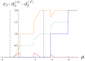
Figure 3: Illustration of the Cooper pair condensate density $\textit{r}_{\beta}$ (red), the “s”–fermion  density $\textit{d}_{\beta}^{\left(\textit{s}\right)}$ (orange), and the “f”–fermion density $\textit{d}_{\beta}^{\left(\textit{f}\right)}$ (blue) for $\beta=200$, $\gamma_{\textit{s}}=3.2$, $\delta=-0.5$, $\lambda_{\textit{s}}=\lambda_{\textit{f}}=1$, $\lambda=0.85$, $h_{\textit{s}}=h_{\textit{f}}=\eta=0$, and $\mu_{\textit{s}}\in\left[-2,7\right]$. The dashed green line corresponds to the average density $\textit{d}_{\beta}:=(\textit{d}_{\beta}^{\left(\textit{s}\right)}+\textit{d}_{\beta}^{\left(\textit{f}\right)})/2$. We concentrate our study between both vertical dashed black lines $\mu_{\textit{s}}=-1$ and $\mu_{\textit{s}}=3$.

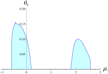
Figure 4: Illustration of the critical temperature $\theta_{c}$ for $\gamma_{\textit{s}}=3.2$, $\delta=-0.5$, $\lambda_{\textit{s}}=\lambda_{\textit{f}}=1$, $\lambda=0.85$, $h_{\textit{s}}=h_{\textit{f}}=\eta=0$, and $\mu_{\textit{s}}\in\left[-1,3\right]$.

Nevertheless, this prediction is not correct. Indeed, for $\mu_{\mathrm{s}}\in\left[-1,3\right]$ the critical temperatures $\theta_{c}$ of superconductivity for $\mathit{d}_{\beta}^{\left(\mathit{s}\right)}>1$ are generally lower than the ones for $\mathit{d}_{\beta}^{\left(\mathit{s}\right)}<1$, see Fig. 4. This asymmetry below and above half–filling results from the (screened) Coulomb interaction (13) together with thermal excitations of “$\mathit{s}$”–fermions into the – here energetically higher ($\delta<0$) – “$\mathit{f}$”–band as one can see from Fig. 5 (which represents the case of an inverse temperature $\beta=11$). In fact, for higher temperatures (lower $\beta$) and $\mathit{d}_{\beta}^{\left(\mathit{s}\right)}>1$ the superconducting phase completely disappears, whereas for $\mathit{d}_{\beta}^{\left(\mathit{s}\right)}<1$, the $U(1)$–broken phase is still found. See Fig. 6 which corresponds to the case $\beta=9$.

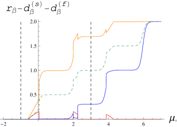
Figure 5: Illustration of the Cooper pair condensate density $\textit{r}_{\beta}$ (red), the “s”–fermion density $\textit{d}_{\beta}^{\left(\textit{s}\right)}$ (orange), and the “f”–fermion density $\textit{d}_{\beta}^{\left(\textit{f}\right)}$ (blue) for $\beta=11$, $\gamma_{\textit{s}}=3.2$, $\delta=-0.5$, $\lambda_{\textit{s}}=\lambda_{\textit{f}}=1$, $\lambda=0.85$, $h_{\textit{s}}=h_{\textit{f}}=\eta=0$, and $\mu_{\textit{s}}\in\left[-2,7\right]$. The dashed green line corresponds to the average density $\textit{d}_{\beta}:=(\textit{d}_{\beta}^{\left(\textit{s}\right)}+\textit{d}_{\beta}^{\left(\textit{f}\right)})/2$. We concentrate our study between both vertical dashed black lines $\mu_{\textit{s}}=-1$ and $\mu_{\textit{s}}=3$.

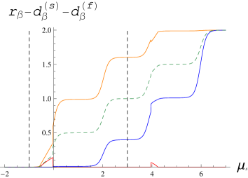
Figure 6: Illustration of the Cooper pair condensate density $\textit{r}_{\beta}$ (red), the “s”–fermion density $\textit{d}_{\beta}^{\left(\textit{s}\right)}$ (orange), and the “f”–fermion density $\textit{d}_{\beta}^{\left(\textit{f}\right)}$ (blue) for $\beta=9$, $\gamma_{\textit{s}}=3.2$, $\delta=-0.5$, $\lambda_{\textit{s}}=\lambda_{\textit{f}}=1$, $\lambda=0.85$, $h_{\textit{s}}=h_{\textit{f}}=\eta=0$, and $\mu_{\textit{s}}\in\left[-2,7\right]$. The dashed green line corresponds to the average density $\textit{d}_{\beta}:=(\textit{d}_{\beta}^{\left(\textit{s}\right)}+\textit{d}_{\beta}^{\left(\textit{f}\right)})/2$. We concentrate our study between both vertical dashed black lines $\mu_{\textit{s}}=-1$ and $\mu_{\textit{s}}=3$.

One clearly sees in Figs. 5 and 6 that at large enough temperature the “$\mathit{f}$”–band is not anymore empty and can inhibit the formation of Cooper pairs in the “$\mathit{s}$”–band because of the Coulomb repulsion (13). This phenomenon can only appear if the critical temperature $\theta_{c}$ is large enough or/and the energy difference $\left|\delta\right|$ is small enough in order to get a non–negligible population of fermions in the “$\mathit{f}$”–band through thermal fluctuations at $\theta\lessapprox\theta_{c}$. Indeed, for large enough $\left|\delta\right|$ the electron–hole asymmetry disappears, i.e., a critical value of the energy gap $\left|\delta\right|$ for electron–hole asymmetry seems to exist, see Fig. 7. If $\delta<0$ and the “$\mathit{f}$”–band is empty at zero temperature then – by a huge amount of numerical experiments – no choice of parameters can favor superconductivity above half–filling, i.e., the maximal critical temperature $\theta_{c}$ is always attained at $\mathit{d}_{\beta}^{\left(\mathit{s}\right)}<1$, as expected.

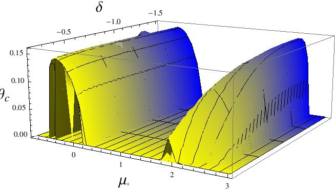
Figure 7: Illustration of the critical temperature $\theta_{c}$ for $\gamma_{\textit{s}}=3.2$, $\lambda_{\textit{s}}=\lambda_{\textit{f}}=1$, $\lambda=0.85$, $h_{\textit{s}}=h_{\textit{f}}=\eta=0$, $\mu_{\textit{s}}\in\left[-1,3\right]$, and $\delta\in\left[-0.2,-1.5\right]$. The color from yellow to blue reflects the increase of the energy gap $|\delta|$.

Observe that the total density of fermions (and not necessarily the chemical potential $\mu_{\mathit{s}}$) should be considered as being a fixed quantity in models for high–$T_{c}$ cuprate superconductors. It is therefore important to check whether the phenomenon described above at fixed chemical potential $\mu_{\mathit{s}}$ is also seen w.r.t. fixed total densities $\rho\in(0,2)$ of fermions or not. Indeed, by strict convexity of the pressure at any finite volume the total density of fermions

$$\mathit{d}_{\beta}:=\frac{1}{2}(\mathit{d}_{\beta}^{\left(\mathit{s}\right)}+\mathit{d}_{\beta}^{\left(\mathit{f}\right)})\in(0,2)$$ (19)

per lattice site and per band is strictly increasing as a function of the chemical potential $\mu_{\mathit{s}}$. Therefore, for any fixed $h_{\mathit{s}},\delta,h_{\mathit{f}},\eta\in\mathbb{R}$, $\gamma_{\mathit{s}},\lambda_{\mathit{s}},\lambda_{\mathit{f}},\lambda\geq 0$, $\beta>0$ and $\rho\in(0,2)$ there exists a unique real number $\mu_{\mathit{s},N,\beta}$ such that

$$\rho = \dfrac{1}{2N}\sum_{x\in\Lambda_{N}}\omega_{N}\left(n_{x,\uparrow}^{(\mathit{s})}+n_{x,\downarrow}^{(\mathit{s})}+n_{x,\uparrow}^{(\mathit{f})}+n_{x,\downarrow}^{(\mathit{f})}\right)$$

$$= \dfrac{1}{2}\omega_{N}\left(n_{x,\uparrow}^{(\mathit{s})}+n_{x,\downarrow}^{(\mathit{s})}+n_{x,\uparrow}^{(\mathit{f})}+n_{x,\downarrow}^{(\mathit{f})}\right),\quad\forall x\in\Lambda_{N},$$

where $\omega_{N}$ represents the (finite volume) grand–canonical Gibbs state (12) associated with $\mathrm{H}_{N}^{(\mathit{s},\mathit{f})}$ and taken at inverse temperature $\beta>0$ and chemical potentials $\mu_{\mathit{s},N,\beta}$ and $\mu_{\mathit{f}}=\mu_{\mathit{s},N,\beta}+\delta$. The Gibbs state $\omega_{N}$ can also in this case be explicitly computed in the limit $N\rightarrow\infty$, see (BruPedra1, , Thm 6.5).

By representing diagrams w.r.t. the parameter $\rho\in(0,1)$ (instead of $\mu_{\mathit{s}}\in\left[-1,3\right])$ we obtain the same kind of behavior as above, see Fig. 8. The only difference to be noted w.r.t. what was already said is the rather frequent coexistence of superconducting and non–superconducting phases at fixed total fermion densities $\rho$ around $0.5$. Indeed, such a coexistence takes place because the chemical potentials to be chosen in order to implement the given densities $\rho$ are such that the parameter vector lies in the set $\mathcal{C}$ of critical points, see Fig. 3. The mathematical proof of coexistence of phases results from a detailed analysis of the (weak^∗–) limit point of $\omega_{N}$ which can be performed exactly as done for the one–band case in (BruPedra1, , Thm. 6.5 (ii)).

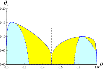
Figure 8: Illustration of the critical temperature $\theta_{c}$ for $\gamma_{\textit{s}}=3.2$, $\delta=-0.5$, $\lambda_{\textit{s}}=\lambda_{\textit{f}}=1$, $\lambda=0.85$, $h_{\textit{s}}=h_{\textit{f}}=\eta=0$, and $\rho\in\left[0,1\right]$. The blue and yellow region correspond respectively to the superconducting and ferromagnetic–superconducting phases. The dashed line corresponds to the absence of doping.

(b) Breakdown of the half–filled “$\mathit{f}$”–band destroying superconductivity:

This situation corresponds to Fig. 9. The interesting interval of chemical potentials is indicated by the dashed black lines $\mu_{\mathit{s}}=1$ and $\mu_{\mathit{s}}=4$. All parameters but the gap $\delta$ are the same as in Fig. 3. Indeed, $\delta=-0.5$ in case (a), whereas $\delta=0.1$ in case (b). With this last choice of parameters the fermion density in the “$\mathit{f}$”–band is now one (instead of zero) at low temperatures. The same phenomenon of asymmetry appears as in case (a) for exactly the same reasons, see Figs. 10 and 11. As in case (a) the maximal critical temperatures for superconductivity are attained at $\mathit{d}_{\beta}^{\left(\mathit{s}\right)}<1$: Superconductivity below half–filling is more favored than superconductivity above half–filling. The converse situation can also appear: At half–filling of the “$\mathit{f}$”–band, maximal critical temperatures are attained at $\mathit{d}_{\beta}^{\left(\mathit{s}\right)}>1$ for other choices of parameters having $\delta<0$ small enough. We omit the details. With the present choice of parameters observe that increasing the mean particle density per site and band over the value $\mathit{d}_{\beta}=1$ causes the collapse – at the same time – of the superconducting phase in the “$\mathit{s}$”–band and of the half–filling in the “$\mathit{f}$”–band, see Fig. 9.

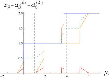
Figure 9: Illustration of the Cooper pair condensate density $\textit{r}_{\beta}$ (red), the “s”–fermion density $\textit{d}_{\beta}^{\left(\textit{s}\right)}$ (orange), and the “f”–fermion density $\textit{d}_{\beta}^{\left(\textit{f}\right)}$ (blue) for $\beta=200$, $\gamma_{\textit{s}}=3.2$, $\delta=0.1$, $\lambda_{\textit{s}}=\lambda_{\textit{f}}=1$, $\lambda=0.85$, $h_{\textit{s}}=h_{\textit{f}}=\eta=0$, and $\mu_{\textit{s}}\in\left[-2,7\right]$. The dashed green line corresponds to the average density $\textit{d}_{\beta}:=(\textit{d}_{\beta}^{\left(\textit{s}\right)}+\textit{d}_{\beta}^{\left(\textit{f}\right)})/2$. We concentrate our study between both vertical dashed black lines $\mu_{\textit{s}}=1$ and $\mu_{\textit{s}}=4$.

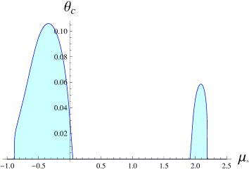
Figure 10: Illustration of the critical temperature $\theta_{c}$ for $\gamma_{\textit{s}}=3.2$, $\delta=0.1$, $\lambda_{\textit{s}}=\lambda_{\textit{f}}=1$, $\lambda=0.85$, $h_{\textit{s}}=h_{\textit{f}}=\eta=0$, and $\mu_{\textit{s}}\in\left[1,4\right]$.

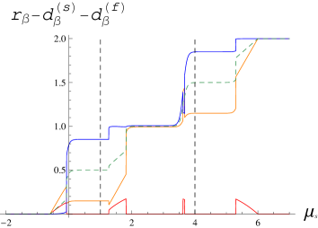
Figure 11: Illustration of the Cooper pair condensate density $\textit{r}_{\beta}$ (red), the “s”–fermion density $\textit{d}_{\beta}^{\left(\textit{s}\right)}$ (orange), and the “f”–fermion density $\textit{d}_{\beta}^{\left(\textit{f}\right)}$ (blue) for $\beta=17.4$, $\gamma_{\textit{s}}=3.2$, $\delta=0.1$, $\lambda_{\textit{s}}=\lambda_{\textit{f}}=1$, $\lambda=0.85$, $h_{\textit{s}}=h_{\textit{f}}=\eta=0$, and $\mu_{\textit{s}}\in\left[-2,7\right]$. The dashed green line corresponds to the average density $\textit{d}_{\beta}:=(\textit{d}_{\beta}^{\left(\textit{s}\right)}+\textit{d}_{\beta}^{\left(\textit{f}\right)})/2$. We concentrate our study between both vertical dashed black lines $\mu_{\textit{s}}=1$ and $\mu_{\textit{s}}=4$.

(c) Breakdown of the half–filled “$\mathit{f}$”–band implying superconductivity:

In this case we analyze the opposite situation to (b): The fact that the breakdown of the half–filling in the “$\mathit{f}$”–band can drive the “$\mathit{s}$”–band into a superconducting phase. This is illustrated in Fig. 12 for $\delta=0.5$ and $\lambda_{\mathit{f}}=1$. It concerns the sector of chemical potentials $\mu_{\mathit{s}}$ for which $\mathit{d}_{\beta}\leq 0.5$, $\mathit{d}_{\beta}$ being the mean particle density (19) per site and per band. This choice of parameters is motivated by the fact that $\lambda_{\mathrm{Cu}}\approx 4\rm{eV}$ and $\delta_{\mathrm{Cu-O}}\leq 0.5\lambda_{\mathrm{Cu}}$ in $\mathrm{CuO}_{2}$ layers of cuprates, see discussions at the beginning of Section II. The most interesting interval of chemical potentials lies between the vertical dashed black lines $\mu_{\mathit{s}}=-1$ and $\mu_{\mathit{s}}=2.5$. This phenomenon is also clearly represented in Fig 13 for $\mathit{d}_{\beta}\leq 0.5$ and a different choice of parameters.

Figure 12: Illustration of the Cooper pair condensate density $\textit{r}_{\beta}$ (red), the “s”–fermion density $\textit{d}_{\beta}^{\left(\textit{s}\right)}$ (orange), and the “f”–fermion density $\textit{d}_{\beta}^{\left(\textit{f}\right)}$ (blue) for $\beta=200$, $\gamma_{\textit{s}}=3.7$, $\delta=0.5$, $\lambda_{\textit{s}}=\lambda_{\textit{f}}=1$, $\lambda=0.85$, $h_{\textit{s}}=h_{\textit{f}}=\eta=0$, and $\mu_{\textit{s}}\in\left[-2,7\right]$. The dashed green line corresponds to the average density $\textit{d}_{\beta}:=(\textit{d}_{\beta}^{\left(\textit{s}\right)}+\textit{d}_{\beta}^{\left(\textit{f}\right)})/2$. We concentrate our study between both vertical dashed black lines $\mu_{\textit{s}}=-1$ and $\mu_{\textit{s}}=2.5$.

In the case $\delta=0.5$, $\lambda_{\mathit{f}}=1$ (Fig. 12) and without any doping, the total density of fermions is one half, i.e., $\mathit{d}_{\beta}=0.5$, and the densities per lattice site of “$\mathit{s}$”– and “$\mathit{f}$”–fermions are respectively $\mathit{d}_{\beta}^{\left(\mathit{s}\right)}=0$ and $\mathit{d}_{\beta}^{\left(\mathit{f}\right)}=1$ (half–filling). Doping the system with additional fermions (holes in the case of cuprates) means that $\mathit{d}_{\beta}>0.5$. This increases the density $\mathit{d}_{\beta}^{\left(\mathit{s}\right)}$ of the “$\mathit{s}$”–band which then becomes superconducting, whereas the “$\mathit{f}$”–band stays half–filled, i.e., $\mathit{d}_{\beta}^{\left(\mathit{f}\right)}=1$. If the total density $\mathit{d}_{\beta}$ is too large ($\mathit{d}_{\beta}\gtrsim 0.73$) then superconductivity is progressively suppressed and the “$\mathit{f}$”–band is not anymore half–filled, i.e., $\mathit{d}_{\beta}^{\left(\mathit{f}\right)}>1$. The physical properties of this (poorly superconducting) phase with $\mathit{d}_{\beta}=1-\varepsilon$ ($\varepsilon=o(1)>0$) are not the same as in the non–superconducting phase with $\mathit{d}_{\beta}=0.5$. The latter is a purely Mott–insulating phase of “$\mathit{f}$”–fermions and the first is a mixture (with fractions depending on the given density $\mathit{d}_{\beta}$)  of a purely Mott–insulating phase of “$\mathit{f}$”–fermions with a phase describing a full “$\mathit{f}$”–band. This is an interesting observation since the excess of doping of holes in real cuprates leads to the destruction of superconductivity and the appearance of a metallic phase, undoped cuprates being Mott insulators. Of course, in our case it is not clear what the thermodynamic phase with $\mathit{d}_{\beta}=1-\varepsilon$ has to do with a metal since no kinetic energy is included and no transport properties are analyzed.

Observe further that such a property is particular to the given choice of parameters. See, e.g., Fig. 13, which corresponds to choose $\delta=0.25$ and $\gamma_{\mathit{s}}=3.2$ (instead of $0.5$ and $3.7$) and where such a phenomenon is not observed around $\mathit{d}_{\beta}\lessapprox 1$.

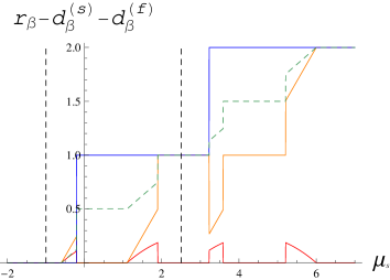
Figure 13: Illustration of the Cooper pair condensate density $\textit{r}_{\beta}$ (red), the “s”–fermion density $\textit{d}_{\beta}^{\left(\textit{s}\right)}$ (orange) and the “f”–fermion density $\textit{d}_{\beta}^{\left(\textit{f}\right)}$ (blue) for $\beta=200$, $\gamma_{\textit{s}}=3.2$, $\delta=0.25$, $\lambda_{\textit{s}}=\lambda_{\textit{f}}=1$, $\lambda=0.85$, $h_{\textit{s}}=h_{\textit{f}}=\eta=0$, and $\mu_{\textit{s}}\in\left[-2,7\right]$. The dashed green line corresponds to the average density $\textit{d}_{\beta}:=(\textit{d}_{\beta}^{\left(\textit{s}\right)}+\textit{d}_{\beta}^{\left(\textit{f}\right)})/2$. We concentrate our study between both vertical dashed black lines $\mu_{\textit{s}}=-1$ and $\mu_{\textit{s}}=2.5$.

Consider again the case $\delta=0.5$ and $\lambda_{\mathit{f}}=1$ of Fig. 12. In contrast to a positive increase of $\mathit{d}_{\beta}$, one does not get a purely superconducting phase by decreasing the total density $\mathit{d}_{\beta}$ of fermions. In fact, similarly to (BruPedra1, , Thm 6.5 (ii)) one sees from Fig. 12 that we have always coexistence of Mott–insulating and superconducting phases for $\mathit{d}_{\beta}\in\left[0.2,0.5\right]$ because of the first order phase transition and density constraints (see below). The fraction of the superconducting phase grows linearly from $0\%$ to $100\%$ when $\mathit{d}_{\beta}$ goes down from $0.5$ to approximately $0.2$. Moreover, as in the other cases we find an asymmetry between superconductivity below and above $\mathit{d}_{\beta}=0.5$ for the half–filled “$\mathit{f}$”–band: It is easier to create a superconducting phase by increasing $\mathit{d}_{\beta}$ than by decreasing $\mathit{d}_{\beta}$, see Fig. 14. As explained in the case (a), this is due to the (screened) Coulomb interaction (13) in interplay with thermal excitations of “$\mathit{f}$”–fermions into the – here energetically higher – “$\mathit{s}$”–level. The latter can be seen from Fig. 15 which corresponds to the inverse temperature $\beta=11$.

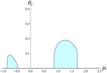
Figure 14: Illustration of the critical temperature $\theta_{c}$ for $\gamma_{\textit{s}}=3.7$, $\delta=0.5$, $\lambda_{\textit{s}}=\lambda_{\textit{f}}=1$, $\lambda=0.85$, $h_{\textit{s}}=h_{\textit{f}}=\eta=0$, and $\mu_{\textit{s}}\in\left[-1,2.5\right]$.

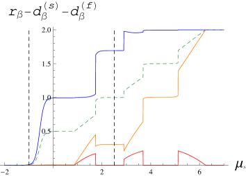
Figure 15: Illustration of the Cooper pair condensate density $\textit{r}_{\beta}$ (red), the “s”–fermion density $\textit{d}_{\beta}^{\left(\textit{s}\right)}$ (orange), and the “f”–fermion density $\textit{d}_{\beta}^{\left(\textit{f}\right)}$ (blue) for $\beta=11$, $\gamma_{\textit{s}}=3.7$, $\delta=0.5$, $\lambda_{\textit{s}}=\lambda_{\textit{f}}=1$, $\lambda=0.85$, $h_{\textit{s}}=h_{\textit{f}}=\eta=0$, and $\mu_{\textit{s}}\in\left[-2,7\right]$. The dashed green line corresponds to the average density $\textit{d}_{\beta}:=(\textit{d}_{\beta}^{\left(\textit{s}\right)}+\textit{d}_{\beta}^{\left(\textit{f}\right)})/2$. We concentrate our study between both vertical dashed black lines $\mu_{\textit{s}}=-1$ and $\mu_{\textit{s}}=2.5$.

By analyzing the model at fixed total densities $\rho\in(0,1)$ of fermions (cf. (III)) we obtain Fig. 16 which represents the critical temperature as a function of $\rho$. It is important to observe that Fig. 16 is qualitatively in accordance with the asymmetry experimentally found in cuprates. See, for instance, the schematic phase diagram of real cuprates reproduced in (Superconductivity3, , Fig. 1).

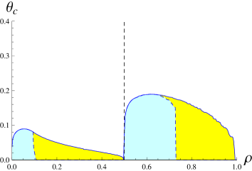
Figure 16: Illustration of the critical temperature $\theta_{c}$ for $\gamma_{\textit{s}}=3.7$, $\delta=0.5$, $\lambda_{\textit{s}}=\lambda_{\textit{f}}=1$, $\lambda=0.85$, $h_{\textit{s}}=h_{\textit{f}}=\eta=0$, and $\rho\in\left[0,1\right]$. The blue and yellow region correspond respectively to the superconducting and ferromagnetic–superconducting phases. The dashed line corresponds to the absence of doping.

Finally, observe that other choices of parameters, specially of the energy gap $\delta$, can completely modify the properties described here, see Figs. 17 and 18.

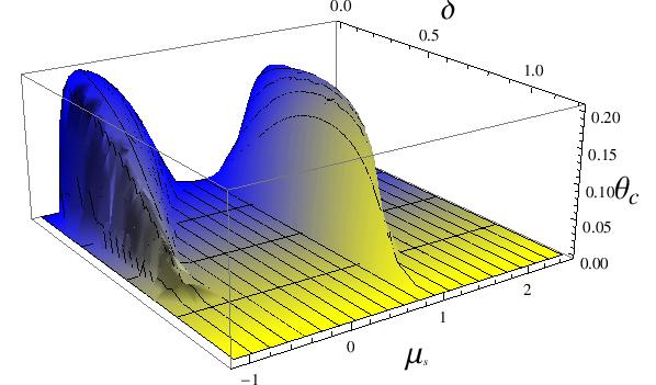
Figure 17: Illustration of the critical temperature $\theta_{c}$ for $\gamma_{\textit{s}}=3.7$, $\lambda_{\textit{s}}=\lambda_{\textit{f}}=1$, $\lambda=0.85$, $h_{\textit{s}}=h_{\textit{f}}=\eta=0$, $\mu_{\textit{s}}\in\left[-1.1,2.5\right]$, and $\delta\in\left[0.,1.2\right]$. The color from blue to yellow reflects the increase of the energy gap $|\delta|$.

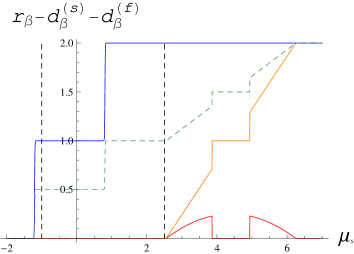
Figure 18: Illustration of the Cooper pair condensate density $\textit{r}_{\beta}$ (red), the “s”–fermion density $\textit{d}_{\beta}^{\left(\textit{s}\right)}$ (orange), and the “f”–fermion density $\textit{d}_{\beta}^{\left(\textit{f}\right)}$ (blue) for $\beta=200$, $\gamma_{\textit{s}}=3.7$, $\delta=1.2$, $\lambda_{\textit{s}}=\lambda_{\textit{f}}=1$, $\lambda=0.85$, $h_{\textit{s}}=h_{\textit{f}}=\eta=0$, and $\mu_{\textit{s}}\in\left[-2,7\right]$. The dashed green line corresponds to the average density $\textit{d}_{\beta}:=(\textit{d}_{\beta}^{\left(\textit{s}\right)}+\textit{d}_{\beta}^{\left(\textit{f}\right)})/2$. We concentrate our study between both vertical dashed black lines $\mu_{\textit{s}}=-1$ and $\mu_{\textit{s}}=2.5$.

(d) The almost full “$\mathit{f}$”–band:

This situation corresponds to Fig. 19. The dashed black lines correspond to the chemical potentials $\mu_{\mathit{s}}=3$ and $\mu_{\mathit{s}}=6.5$. In this case (d) we choose $\delta=0.2$, the other parameters being the same as in cases (a) and (b). The electron–hole asymmetry appears again and exactly for the same reasons, see Figs. 20 and 21. Observe, however, that the fermion density in the “$\mathit{f}$”–band is two (instead of zero or one) at low temperatures. Notice also that – in contrast to the case (a) – the maximal critical temperatures are always attained at $\mathit{d}_{\beta}^{\left(\mathit{s}\right)}>1$. At high enough temperatures the superconducting phase completely disappears for $\mathit{d}_{\beta}^{\left(\mathit{s}\right)}<1$, whereas it can still be found if $\mathit{d}_{\beta}^{\left(\mathit{s}\right)}>1$. I.e., in this situation (d) superconductivity above half–filling is more favored than superconductivity below half–filling. In fact, if $\delta>0$ and the energetically lower level “$\mathit{f}$” is full at zero temperature then no choice of parameters for which the maximum critical temperature is attained at $\mathrm{d}_{\beta}^{\left(\mathit{s}\right)}<1$ were found.

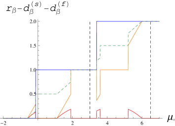
Figure 19: Illustration of the Cooper pair condensate density $\textit{r}_{\beta}$ (red), the “s”–fermion density $\textit{d}_{\beta}^{\left(\textit{s}\right)}$ (orange), and the “f”–fermion density $\textit{d}_{\beta}^{\left(\textit{f}\right)}$ (blue) for $\beta=200$, $\gamma_{\textit{s}}=3.2$, $\delta=0.2$, $\lambda_{\textit{s}}=\lambda_{\textit{f}}=1$, $\lambda=0.85$, $h_{\textit{s}}=h_{\textit{f}}=\eta=0$, and $\mu_{\textit{s}}\in\left[-2,7\right]$. The dashed green line corresponds to the average density $\textit{d}_{\beta}:=(\textit{d}_{\beta}^{\left(\textit{s}\right)}+\textit{d}_{\beta}^{\left(\textit{f}\right)})/2$. We concentrate our study between both vertical dashed black lines $\mu_{\textit{s}}=3$ and $\mu_{\textit{s}}=6.5$.

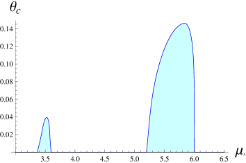
Figure 20: Illustration of the critical temperature $\theta_{c}$ for $\gamma_{\textit{s}}=3.2$, $\delta=0.2$, $\lambda_{\textit{s}}=\lambda_{\textit{f}}=1$, $\lambda=0.85$, $h_{\textit{s}}=h_{\textit{f}}=\eta=0$, and $\mu_{\textit{s}}\in\left[3,6.5\right]$.

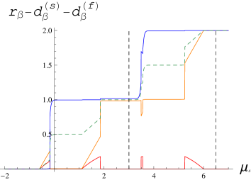
Figure 21: Illustration of the Cooper pair condensate density $\textit{r}_{\beta}$ (red), the “s”–fermion density $\textit{d}_{\beta}^{\left(\textit{s}\right)}$ (orange), and the “f”–fermion density $\textit{d}_{\beta}^{\left(\textit{f}\right)}$ (blue) for $\beta=28$, $\gamma_{\textit{s}}=3.2$, $\delta=0.2$, $\lambda_{\textit{s}}=\lambda_{\textit{f}}=1$, $\lambda=0.85$, $h_{\textit{s}}=h_{\textit{f}}=\eta=0$, and $\mu_{\textit{s}}\in\left[-2,7\right]$. The dashed green line corresponds to the average density $\textit{d}_{\beta}:=(\textit{d}_{\beta}^{\left(\textit{s}\right)}+\textit{d}_{\beta}^{\left(\textit{f}\right)})/2$. We concentrate our study between both vertical dashed black lines $\mu_{\textit{s}}=3$ and $\mu_{\textit{s}}=6.5$.

Cases (b) and (d) can also be considered – as it was done for the cases (a) and (c) – w.r.t. a fixed total fermion density $\rho\in(0,2)$ (instead of a fixed chemical potential $\mu_{\mathit{s}}$), see (III). All phenomena concerning the electron–hole asymmetry described at fixed $\mu_{\mathit{s}}$ also appear at fixed $\rho\in(0,2)$ completely analogously to the cases (a) and (c). A detailed analysis is therefore omitted.

From the physical description given at the beginning of Section II, cuprates seem to fit in case (c) since $\delta>0$ whereas $\mathit{d}_{\beta}^{\left(\mathit{f}\right)}=1$ and $\mathit{d}_{\beta}^{\left(\mathit{s}\right)}=0$ at $\mathit{d}_{\beta}=0.5$ (no doping). In this case the non–superconducting band (“$\mathit{f}$”–band) should be identified with copper orbitals – which is half–filled without doping – and the superconducting band (“$\mathit{s}$”–band) with oxygen orbitals – which is empty without doping. Note that experiments indicate that superconduction takes place in oxygen orbitals (see Section 5.11 of Saxena ). Considering Hamiltonians for holes in cuprates, our model correctly predicts (see case (c)) that if $\delta>0$ (i.e., if holes in oxygen orbitals are higher in energy than holes in copper orbitals, which is the case in real cuprates), then the highest critical temperature is obtained at $\mathit{d}_{\beta}^{\left(\mathit{s}\right)}>1$, i.e., by introducing donors of holes in the cuprate crystal.

Note finally that the phenomenon of electron–hole asymmetry can also take place if the inter–band interaction is purely magnetic (instead of purely electrostatic) or is mixed (i.e., has magnetic and electrostatic components). As in cases (a) or (d) one can find examples where the maximal critical temperature of superconductivity is either at $\mathit{d}_{\beta}^{\left(\mathit{s}\right)}<1$ or at $\mathit{d}_{\beta}^{\left(\mathit{s}\right)}>1$. See, e.g., Figs. 22 and 23. Moreover, in the case of a non–vanishing magnetic inter–band interaction

$$-\eta\sum_{x\in\Lambda_{N}}(n_{x,\uparrow}^{(\mathit{s})}-n_{x,\downarrow}^{(\mathit{s})})(n_{x,\uparrow}^{(\mathit{f})}-n_{x,\downarrow}^{(\mathit{f})})$$ (21)

a new phenomenon takes place: The so–called reentering behavior which is analyzed below in more details.

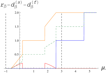
Figure 22: Illustration of the Cooper pair condensate density $\textit{r}_{\beta}$ (red), the “s”–fermion density $\textit{d}_{\beta}^{\left(\textit{s}\right)}$ (orange), and the “f”–fermion density $\textit{d}_{\beta}^{\left(\textit{f}\right)}$ (blue) for $\beta=2000$, $\gamma_{\textit{s}}=3.2$, $\delta=-2.6$, $\lambda_{\textit{s}}=\lambda_{\textit{f}}=1$, $\eta=0.5$, $h_{\textit{s}}=h_{\textit{f}}=\lambda=0$, and $\mu_{\textit{s}}\in\left[-1,5.5\right]$. The dashed green line corresponds to the average density $\textit{d}_{\beta}:=(\textit{d}_{\beta}^{\left(\textit{s}\right)}+\textit{d}_{\beta}^{\left(\textit{f}\right)})/2$. We concentrate our study between both vertical dashed black lines $\mu_{\textit{s}}=-1$ and $\mu_{\textit{s}}=3$.

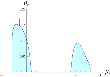
Figure 23: Illustration of the critical temperature $\theta_{c}$ for $\gamma_{\textit{s}}=3.2$, $\delta=-2.6$, $\lambda_{\textit{s}}=\lambda_{\textit{f}}=1$, $\eta=0.5$, $h_{\textit{s}}=h_{\textit{f}}=\lambda=0$, and $\mu_{\textit{s}}\in\left[-1,3\right]$.

IV Reentering behavior and magnetic inter–band interaction

We fix $\eta\neq 0$ in (9). Otherwise the reentering behavior would not take place. Since we are only interested on effects due to the magnetic inter–band interaction (21) on the superconductivity of “$\mathit{s}$”–fermions we let $\lambda=0$ in (9). A small electrostatic component $\lambda\simeq 0$ does not change the qualitative thermodynamic behavior of the model.

An illustration of the Cooper pair condensate density as well as the critical temperature w.r.t. the chemical potential $\mu_{\mathit{s}}$ of “$\mathit{s}$”–fermions  is given for this situation in Figs. 24 and 25. It is interesting to observe that a reentering behavior occurs: At $\mu_{\mathit{s}}=0.4$ (dashed line in Fig. 25) the system becomes superconducting below a critical temperature $\theta_{c_{1}}$ and then leaves the superconducting phase below $\theta_{c_{2}}$ with $\theta_{c_{2}}<\theta_{c_{1}}$. This kind of phenomenology is found in real ferromagnetic superconductors (Shrivastava, , p. 263-267).

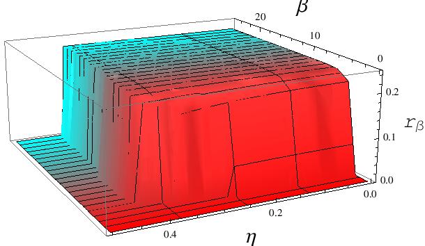
Figure 24: Illustration, as a function of $\eta\in\left[0,0.5\right]$ and $\beta\in\left[0.1,25\right]$, of the Cooper pair condensate density $\textit{r}_{\beta}$ for $\gamma_{\textit{s}}=3.2$, $\lambda_{\textit{s}}=\lambda_{\textit{f}}=0.5$, $\mu_{\textit{s}}=\mu_{\textit{f}}=1$ and $h_{\textit{s}}=h_{\textit{f}}=\lambda=0$. The color from red to blue reflects the decrease of the temperature.

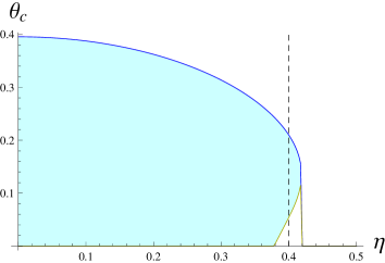
Figure 25: Illustration of the domain of temperature (blue region) with a superconducting phase for $\gamma_{\textit{s}}=3.2$, $\lambda_{\textit{s}}=\lambda_{\textit{f}}=0.5$, $\mu_{\textit{s}}=\mu_{\textit{f}}=1$, $h_{\textit{s}}=h_{\textit{f}}=\lambda=0$, and $\eta\in\left[0,0.5\right]$. For, e.g., $\eta=0.4$ (black dashed line) a reentering behaviour appears.

The total magnetization density per band

$$\mathit{m}_{\beta}:=\underset{N\rightarrow\infty}{\lim}\omega_{N}\left(n_{x,\uparrow}^{(\mathit{s})}-n_{x,\downarrow}^{(\mathit{s})}+n_{x,\uparrow}^{(\mathit{f})}-n_{x,\downarrow}^{(\mathit{f})}\right)$$

($\mathit{m}_{\beta}\in[-1,1]$) equals

$$\mathit{m}_{\beta} = \frac{e^{-2\beta\lambda}}{\mathrm{f}(\mathit{r}_{\beta})}\Bigl{\{}4\mathrm{e}^{\beta\eta}\sinh\left(\beta\left(h_{\mathit{f}}+h_{\mathit{s}}\right)\right)$$ (22)

$$+(\mathrm{e}^{-\beta\left(\mu_{\mathit{f}}-2\lambda\right)}+\mathrm{e}^{-\beta(2\lambda+2\lambda_{\mathit{f}}-\mu_{\mathit{f}})})\sinh(\beta h_{\mathit{s}})$$

$$+2\mathrm{e}^{-\beta\lambda_{\mathit{s}}}\cosh(\beta g_{r,2\lambda})\sinh(\beta h_{\mathit{f}})\Bigr{\}}$$

away from any critical point. In particular, – in contrast to what is observed in real ferromagnetic superconductors – no spontaneous magnetization can occur in this model, as the Hamiltonian is invariant under exchange of $\uparrow$ and $\downarrow$ spins for $h_{\mathit{s}}=h_{\mathit{f}}=0$. A more complicated model including, for instance, Heisenberg–type intra–band interaction terms could show spontaneous magnetization. In order to simplify the analysis we induce magnetization by imposing a small external magnetic field $h_{\mathit{f}}\neq 0.$ See Fig. 26. In this case we obtain some (poorly) ferromagnetic superconducting phase at fixed chemical potential. In contrast to models showing spontaneous magnetization and real ferromagnetic superconductors, this procedure has of course the drawback of implying – at any fixed temperature – small magnetizations at small fields $h_{\mathit{f}},h_{\mathit{s}}$, i.e., $|\mathit{m}_{\beta}|=O(|h_{\mathit{f}}|+|h_{\mathit{s}}|)$, see Fig. 26. For more details we recommend (BruPedra1, , Sect. 3.3).

Proceeding in this way the total magnetization density $\mathit{m}_{\beta}$ in the superconducting phase generally stays rather small: In Fig. 26 $\mathit{m}_{\beta}$ is at most 23% of $\mathit{r}_{\beta}$ in the superconducting phase. However, $\mathit{m}_{\beta}$ is increased by almost 600% at the lowest critical temperature of superconductivity. This captures in a sense the property of real ferromagnetic superconductors of going into a ferromagnetic phase when they leave the superconducting phase at low temperatures (i.e., below the critical temperature $\theta_{c_{2}}$).

Note that, if the range of temperatures with a superconducting phase is sufficiently small then the magnetization $\mathit{m}_{\beta}$ (in the superconducting phase) becomes almost zero, see, e.g., (BruPedra1, , Corollary 3.3). There is also a critical magnetic field $|h_{\mathit{s}}^{\left(c\right)}|$ above which the superconducting phase cannot exist at any temperature: This can be seen as (part of) the usual Meißner effect.

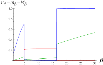
Figure 26: Illustration of the Cooper pair condensate density $\textit{r}_{\beta}$ (red), the intra-band magnetization density $\mathrm{m}_{\beta}$ (green), and the inter-band magnetization density $\mathrm{M}_{\beta}$ (blue) for $\gamma_{\textit{s}}=3.2$, $\lambda_{\textit{s}}=\lambda_{\textit{f}}=0.5$, $\mu_{\textit{s}}=\mu_{\textit{f}}=1$, $\eta=0.4$, $h_{\textit{s}}=h_{\textit{f}}=0.01$, $\lambda=0$, and $\beta\in\left[1,30\right]$.

The inter–band magnetization density

$$\mathit{M}_{\beta}:=\underset{N\rightarrow\infty}{\lim}\omega_{N}\left((n_{x,\uparrow}^{(\mathit{f})}-n_{x,\downarrow}^{(\mathit{f})})(n_{x,\uparrow}^{(\mathit{s})}-n_{x,\downarrow}^{(\mathit{s})})\right)$$

($\mathit{M}_{\beta}\in[-1,1]$) equals

$$\mathit{M}_{\beta} = \frac{e^{-2\beta\lambda}}{\mathrm{f}(\mathit{r}_{\beta})}\Bigl{\{}\mathrm{e}^{-\beta h_{\mathit{s}}}\sinh(\beta(\eta-h_{\mathit{f}}))$$ (23)

$$+\mathrm{e}^{\beta h_{\mathit{s}}}\sinh\left(\beta(\eta+h_{\mathit{f}})\right)\Bigr{\}}$$

away from any critical point. In the superconducting phase, 100% of “$\mathit{s}$”–fermions form Cooper pairs in the limit of zero–temperature ($\beta\rightarrow\infty$). This implies that $\mathit{M}_{\beta}=0$ in this limit. See Figs. 24 and 27 as well as Fig. 28. Moreover, because of symmetries of the model, the magnetic inter–band interaction (21) is always zero at $h_{\mathit{s}}=h_{\mathit{f}}=0$. Thus, one could think that the magnetic interaction does not perturb much the superconducting phase of “$\mathit{s}$”–fermions. It turns out that the thermodynamic effect of the magnetic inter–band coupling is by far not negligible: It can even completely destroy the superconducting phase, either at low enough temperature, or for any temperature when $|\eta|>\eta_{\infty}^{(c)}$. In particular, the two–band model discussed here shows a reentering behavior also without any external magnetic field (and thus, without ferromagnetism), see Fig. 28. Indeed, at any fixed inverse temperature $\beta>0$ there is a critical magnetic inter–band interaction $\eta_{\beta}^{(c)}$ such that the superconducting phase disappears for $|\eta|>\eta_{\beta}^{(c)}$, even if there is no magnetization, see Fig. 25.

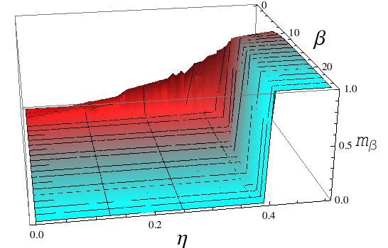
Figure 27: Illustration of the inter–band magnetization density $\mathrm{M}_{\beta}$ for $\gamma_{\textit{s}}=3.2$, $\lambda_{\textit{s}}=\lambda_{\textit{f}}=0.5$, $\mu_{\textit{s}}=\mu_{\textit{f}}=1$ and $h_{\textit{s}}=h_{\textit{f}}=\lambda=0$, $\eta\in\left[0,0.5\right]$, and $\beta\in\left[0.1,25\right]$. The color from red to blue reflects the decrease of the temperature.

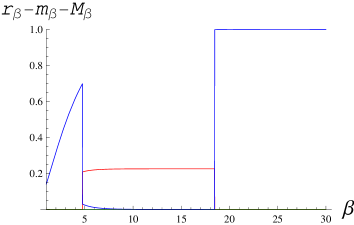
Figure 28: Illustration of the Cooper pair condensate density $\textit{r}_{\beta}$ (red), the intra-band magnetization density $\mathrm{m}_{\beta}$ (green), and the inter-band magnetization density $\mathrm{M}_{\beta}$ (blue) for $\gamma_{\textit{s}}=3.2$, $\lambda_{\textit{s}}=\lambda_{\textit{f}}=0.5$, $\mu_{\textit{s}}=\mu_{\textit{f}}=1$, $\eta=0.4$, $h_{\textit{s}}=h_{\textit{f}}=\lambda=0$, and $\beta\in\left[1,30\right]$.

Note that the reentering behavior does not seem to appear at fixed densities $\rho^{\left(\mathit{f}\right)}\in\left(0,2\right)$ of “$\mathit{f}$”–fermions, which uniquely define at fixed $\mu_{\mathit{s}}\in\mathbb{R}$ a chemical potential $\mu_{\mathit{f}\mathrm{,}N,\beta}$ for any $N\in\mathbb{N}$ such that

$$\rho^{\left(\mathit{f}\right)}=\omega_{N}\left(n_{x,\uparrow}^{(\mathit{f})}+n_{x,\downarrow}^{(\mathit{f})}\right).$$

Therefore, if the two–band model $\mathrm{H}_{N}^{(\mathit{s},\mathit{f})}$ is supposed to describe a system of fixed (fermionic) atoms (playing the role of “$\mathit{f}$”–fermions) and moving fermions (“$\mathit{s}$”–fermions), then the model does not seem – in this situation – to show the reentering behavior for any choice parameters.

At fixed total fermion density $\rho\in\left(0,2\right)$ (cf. (III)) we have found that the reentering behavior does not appear unless $\rho=1$. Indeed, if $\rho=1$, then – up to numerical aberrations we might not see – the two–band model seems to show, surprisingly, a reentering behavior in pretty good accordance with the phenomenology of ferromagnetic superconductors (see Figs. 29 and 30):

• At all temperatures $\theta>\theta_{c_{1}}\simeq 0.28$, the system is not superconducting.

• At all temperatures $\theta\in(\theta_{c_{2}},\theta_{c_{1}}]$ with $\theta_{c_{2}}\simeq 0.09$, the system is superconducting.

• At temperatures $\theta\in(\theta_{c_{3}},\theta_{c_{2}})$ with $\theta_{c_{3}}\simeq 0.06$, a coexistence of the non–superconducting (which is magnetic in the presence of any non–vanishing external magnetic field) and superconducting phases appears. This seems to be the case in real ferromagnetic superconductors, cf. (Shrivastava, , p. 263-267).

• At all temperatures $\theta\leq\theta_{c_{3}}$, there is a non–superconducting – ferromagnetic in presence of non–zero external magnetic fields – phase.

Note that the possible choices of parameters leading to this peculiar behavior seems to be relatively rare.

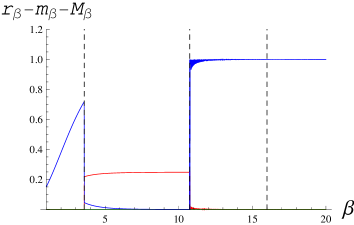
Figure 29: Illustration of the Cooper pair condensate density $\textit{r}_{\beta}$ (red), the intra-band magnetization density $\mathrm{m}_{\beta}$ (green), and the inter-band magnetization density $\mathrm{M}_{\beta}$ (blue) for $\gamma_{\textit{s}}=3.54$, $\lambda_{\textit{s}}=\lambda_{\textit{f}}=0.5$, $\delta=-0.5$, $h_{\textit{s}}=h_{\textit{f}}=\lambda=0$, $\eta=0.4$, $\rho=1$, and $\beta\in\left[1,20\right]$. A coexistence of phases takes place for inverse temperatures $\beta\in(\beta_{c_{2}},\beta_{c_{3}})$ with $\beta_{c_{2}}\simeq 10.75$ and $\beta_{c_{3}}\simeq 16$.

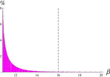
Figure 30: % of the superconducting phase for $\gamma_{\textit{s}}=3.54$, $\lambda_{\textit{s}}=\lambda_{\textit{f}}=0.5$, $\delta=-0.5$, $h_{\textit{s}}=h_{\textit{f}}=\lambda=0$, $\eta=0.4$, $\rho=1$, and $\beta\in(10.8,20)$. The black dashed line corresponds to $\beta=\beta_{c_{3}}\simeq 16$.

At fixed chemical potentials or at fixed total fermion density per band exactly equal one and if the parameters are chosen such that the reentering behavior takes place, then we observe the following property of the non–superconducting phase at low temperatures: The probability of finding exactly one “$\mathit{s}$”–fermion and exactly one “$\mathit{f}$”–fermion on a given lattice site goes to one as $\beta\rightarrow\infty$. This can be interpreted as follows: At low temperatures there is formation of pairs composed by one “$\mathit{s}$”–fermion and one “$\mathit{f}$”–fermion, a sort of magnetic bound state (for instance, some kind of Kondo bound state). These pairs form in turn a Mott phase. This mechanism of “$\mathit{sf}$”–pairing could be an explanation for the disappearing of the superconducting phase. Apparently, destroying such pairs in order to set “$\mathit{s}$”–fermions free to form Cooper pairs is energetically not favorable at low temperatures.

V Appendix

Thermodynamic properties of Hamiltonians of the form

$$H_{N,\gamma}:=H_{N}-\frac{\gamma}{N}\sum_{x,y\in\Lambda_{N}}a_{x,\uparrow}^{\ast}a_{x,\downarrow}^{\ast}a_{y,\downarrow}a_{y,\uparrow}\otimes\mathbf{1}$$

acting on the tensor product of Fock spaces of “$\mathit{s}$”– and “$\mathit{f}$”–fermions can be analyzed by the approximating Hamiltonians

$$H_{N,\gamma}\left(c\right) : =H_{N}$$

$$-\frac{\gamma}{N}\sum_{x\in\Lambda_{N}}\left(\left(Nc\right)a_{x,\uparrow}^{\ast}a_{x,\downarrow}^{\ast}+\left(N\bar{c}\right)a_{x,\downarrow}a_{x,\uparrow}\right)\otimes\mathbf{1}$$

with $c\in\mathbb{C}$ conveniently chosen. This procedure is known in mathematical physics as the “approximating Hamiltonian method” approx-hamil-method . This was shown to be exact for a large class of models on the level of the grand–canonical pressure as soon as one maximizes over $c\in\mathbb{C}$ the (infinite volume) pressure associated with $H_{N,\gamma}\left(c\right)$, see approx-hamil-method ; BruPedra2 . The maximizers of the $c$–depending pressures are solutions of Euler–Lagrange equations called gap equations.

Applying this method to the model $\mathrm{H}_{N}^{(\mathit{s},\mathit{f})}$ one obtains Theorem 1 because the approximating Hamiltonian $\mathrm{H}_{N}^{(\mathit{s},\mathit{f})}\left(c\right)$ is a (tensor product of the same) ($16\times 16)$–matrix which can be exactly diagonalized. In particular, its pressure $p(c)$ can explicitly be computed for all $c\in\mathbb{C}$. Since $\mathrm{H}_{N}^{(\mathit{s},\mathit{f})}$ is gauge invariant it suffices to restrict the variational problem to positive real numbers $r:=|c|^{2}\geq 0$. For more details we recommend BruPedra1 . In case of interest, see also BruPedra2 where this theory is developed in a much more general setting.

Proofs of (16), (17), (18), (22), and (23) follow from a study of equilibrium states of the model, see BruPedra1 ; BruPedra2 . Heuristically, they can be obtained by using a rather old method: Griffiths arguments which are based on convexity properties of the pressure, see (BruPedra1, , Section 8). The drawback of Griffiths arguments is that it requires the differentiability of the order parameter $\mathit{r}_{\beta}$ w.r.t. perturbations corresponding to the observable to be analyzed. The latter represents often a difficult task and is generally even wrong at critical points. Forgetting this problem for a moment we can compute all expectation values. For instance, Griffiths arguments tell us that

$$\underset{N\rightarrow\infty}{\lim}\left\{N^{-1}\omega_{N}\left(\mathfrak{c}_{0}^{\ast}\mathfrak{c}_{0}\right)\right\}=\partial_{\gamma}\mathrm{p|}_{\mathit{r}_{\beta}}=\mathit{r}_{\beta}$$

because of the Euler–Lagrange (gap) equation (14). Similarly, $\mathit{d}_{\beta}^{\left(\mathit{s}\right)}=\partial_{\mu_{\mathit{s}}}\mathrm{p|}_{\mathit{r}_{\beta}}$, $\mathit{d}_{\beta}^{\left(\mathit{f}\right)}=\partial_{\mu_{\mathit{f}}}\mathrm{p|}_{\mathit{r}_{\beta}}$, $\mathit{m}_{\beta}=\partial_{h_{\mathit{f}}}\mathrm{p|}_{\mathit{r}_{\beta}}+\partial_{h_{\mathit{s}}}\mathrm{p|}_{\mathit{r}_{\beta}}$ and $\mathit{M}_{\beta}=\partial_{\eta}\mathrm{p|}_{\mathit{r}_{\beta}}$. Computing all these derivatives by using the gap equation (14) one obtains Equations (16), (17), (18), (22), and (23).

One of the main achievements of BruPedra1 ; BruPedra2 was to develop a method to overcome the differentiability needed in Griffiths arguments. The method of BruPedra1 ; BruPedra2 permits, moreover, to represent equilibrium states of models in an efficient way. This makes, among other things, the analysis of arbitrary correlation functions and the study of equilibrium states at fixed fermion densities possible.
Acknowledgments: We thank M. Salmhofer for interesting discussions and encouragement as well as E. Sherman for giving us interesting references and remarks. The two first authors were supported by the grant MTM2010-16843 of the Spanish “Ministerio de Ciencia e Innovación”, the third author by a grant of the “Inneruniversitäre Forschungsförderung” of the Johannes Gutenberg University in Mainz.

References

- (1) J.-B. Bru and W. de Siqueira Pedra, Rev. Math. Phys. 22, 233 (2010).
- (2) D. J. Thouless, The Quantum Mechanics of Many–Body Systems. Second Edition (Academic Press, New York, 1972).
- (3) N. N. Bogoliubov, V.V. Tolmachev, and D. V. Shirkov, A New Method in the Theory of Superconductivity (Academy of Sciences Press, Moscow, 1958) or (Consult.Bureau, Inc., N.Y., Chapman Hall Ltd., London, 1959).
- (4) Y. Yanase, T. Jujo, T. Nomura, H. Ikeda, T. Hotta, and K. Yamada, Physics Reports 387, 1 (2003).
- (5) P. A. Lee, N. Nagaosa, and X.-G. Wen, Rev. Mod. Phys. 78, 17 (2006).
- (6) R. J. Bursill and C. J. Thompson, J. Phys. A Math. Gen. 26, 4497 (1993).
- (7) F. P. Mancini, F. Mancini, and A. Naddeo, Journal of optoelectronics and advanced materials 10, 1688 (2008).
- (8) V. J. Emery, Phys. Rev. Lett. 58, 2794 (1987).
- (9) K. N. Shrivastava, Superconductivity: Elementary Topics (World Scientific: Singapore, New Jersey, London, Hong Kong, 2000).
- (10) A. K. Saxena, High-Temperature Superconductors (Springer-Verlag, Berlin Heildelberg, 2010).
- (11) E. H. Lieb, Phys. Rev. Lett. 62, 1201 (1989).
- (12) G.-S. Tian, J. Stat. Phys. 116, 629 (2004).
- (13) N. N. Bogoliubov Jr., J. G. Brankov, V. A. Zagrebnov, A. M. Kurbatov, and N. S. Tonchev, Russ. Math. Surv. 39, 1 (1984).
- (14) J.-B. Bru and W. de Siqueira Pedra, Non–cooperative Equilibria of Fermi Systems With Long Range Interactions. Memoirs of the AMS 224 (2013), no. 1052.